Complex potential well
a research training report by Max Lewandowski
July 26, 2011
Supervisor: Priv.-Doz. Dr. Axel Pelster
1
Contents
1 Introduction 3
2 Complex 1-dimensional square well potential 5
2.1 Schrödinger equation . . . . . . . . . . . . . . . . . . . . . . . . . . . . . . . . . . 6
2.2 Continuity equation . . . . . . . . . . . . . . . . . . . . . . . . . . . . . . . . . . . 7
2.3 Static solutions . . . . . . . . . . . . . . . . . . . . . . . . . . . . . . . . . . . . . 9
2.4 Symmetric states . . . . . . . . . . . . . . . . . . . . . . . . . . . . . . . . . . . . 11
2.4.1 Real limit . . . . . . . . . . . . . . . . . . . . . . . . . . . . . . . . . . . . 13
2.4.2 Limit of vanishing waist . . . . . . . . . . . . . . . . . . . . . . . . . . . . 15
2.5 Antisymmetric states . . . . . . . . . . . . . . . . . . . . . . . . . . . . . . . . . . 16
2.5.1 Real limit . . . . . . . . . . . . . . . . . . . . . . . . . . . . . . . . . . . . 17
2.5.2 Limit of vanishing waist . . . . . . . . . . . . . . . . . . . . . . . . . . . . 19
3 Numerical analysis 20
3.1 Some further theoretical discussion . . . . . . . . . . . . . . . . . . . . . . . . . . 20
3.1.1 Dimensionless variables . . . . . . . . . . . . . . . . . . . . . . . . . . . . . 20
3.1.2 Limit of big waist . . . . . . . . . . . . . . . . . . . . . . . . . . . . . . . . 21
3.2 Energies . . . . . . . . . . . . . . . . . . . . . . . . . . . . . . . . . . . . . . . . . 22
3.2.1 Solutions . . . . . . . . . . . . . . . . . . . . . . . . . . . . . . . . . . . . . 22
3.2.2 Saturation value for real part of energy . . . . . . . . . . . . . . . . . . . . 26
3.2.3 Discussion . . . . . . . . . . . . . . . . . . . . . . . . . . . . . . . . . . . . 29
3.3 Densities . . . . . . . . . . . . . . . . . . . . . . . . . . . . . . . . . . . . . . . . . 31
3.3.1 Solutions . . . . . . . . . . . . . . . . . . . . . . . . . . . . . . . . . . . . . 31
3.3.2 Discussion . . . . . . . . . . . . . . . . . . . . . . . . . . . . . . . . . . . . 37
3.3.3 Critical waists . . . . . . . . . . . . . . . . . . . . . . . . . . . . . . . . . . 38
3.4 Currents . . . . . . . . . . . . . . . . . . . . . . . . . . . . . . . . . . . . . . . . . 40
3.4.1 Solutions . . . . . . . . . . . . . . . . . . . . . . . . . . . . . . . . . . . . . 40
3.4.2 Discussion . . . . . . . . . . . . . . . . . . . . . . . . . . . . . . . . . . . . 46
4 Outlook 47
4.1 Time evolution and interpretation of imaginary energies . . . . . . . . . . . . . . . 47
4.2 Determination of critical waist . . . . . . . . . . . . . . . . . . . . . . . . . . . . . 47
4.3 More accurate derivation of real part of energy . . . . . . . . . . . . . . . . . . . . 48
4.4 Further discussion of densities and currents . . . . . . . . . . . . . . . . . . . . . . 48
4.5 Evaluation of higher states . . . . . . . . . . . . . . . . . . . . . . . . . . . . . . . 48
4.6 More general approach . . . . . . . . . . . . . . . . . . . . . . . . . . . . . . . . . 48
2

1 Introduction
Already in 1924 Satyendranath Bose wrote a paper where he used a novel way for counting states
of identical photons to derive Planck's quantum radiation law. In this way he found out that the
Maxwell-Boltzmann distribution is not true for microscopic particles and has to be replaced by
another distribution [1]. In the same year this idea was extended to massive particles by Albert
Einstein [2], therefore this new distribution is called Bose-Einstein distribution. It predicts a
macroscopic occupation of the ground state by a dense collection of particles with integer spin,
called bosons, for very low temperatures near to absolute zero. This phenomenon is called Bose-
Einstein condensation. The �rst experimental realization of a pure Bose-Einstein condensate
(BEC) was accomplished in 1995 by Eric Cornell and Carl Wieman at JILA [3] and Wolfgang
Ketterle at MIT [4]. The creation of a BEC requires temperatures very near absolute zero to reach
the critical temperature for the phase transition. The new techniques of laser cooling [5�7] and
magnetic evaporative cooling [8] made it possible for E. Cornell and C. Wiedman to cool down
a gas of rubidium-87 atoms con�ned in a magnetic time-averaged, orbital potential (TOP) trap
to 170 nanoKelvin which undermatches the critical temperature of 87Rb. In the same year W.
Ketterle produced at MIT a much larger BEC of sodium-23, which allowed him to observe even
�rst coherence e�ects like the quantum mechanical interference between two di�erent BECs [9].
So far BECs have been created with many other kinds of atoms like 1H, 7Li, 23Na, 39K,41K, 52Cr, 85Rb, 87Rb, 133Cs, 170Yb, 174Yb and 4He in an excited state. Moreover, experiments
with BEC as well as its theory became one of the most interesting physical research topics in
the last years like the realization of a BEC in optical lattices which are standing laser �elds
that yield via the AC Stark e�ect periodic potential wells for atoms [10, 11]. This leads to a
strongly correlated BEC which is well controlled by the respective laser parameters and yields
for increasing laser intensities a quantum phase transition from the super�uid to a Mott phase.
As the latter is characterized by a �xed number of bosons in each well, a Bose gas in an optical
lattice is a promising candidate for quantum simulations like entanglement of atoms or quantum
teleportation [12]. Also disordered Bose gases can be realized via laser speckles or incommensurable
optical lattices to create random potentials [13]. Another interesting research �eld are fermionic
condensates. Two weakly correlated fermions called Cooper pairs yield a "particle" with integer
spin which therefore also obeys Bose-Einstein statistics despite the fermionic constituents. By
increasing the correlation for example by a magnetic trap there is a phase transition from this
BCS phase of weakly coupled fermions [14] to bound boson molecules condensing to a BEC, which
is called BCS-BEC-crossover [15].
Furthermore, complex potentials are used in a BEC as a heuristic tool to model dissipation
processes which occur once a BEC is brought in contact, for instance, with an ion [18]. This
research work is related to an experiment performed by Herwig Ott [16, 17] from the Technical
University of Kaiserslautern where a Rb87-BEC interacts with an electron beam according to
Fig. 1, which is one technique to achieve single-site adressabilities [19�22].
3

Figure 1: The atomic ensemble is prepared in an optical dipole trap. An electron beam withvariable beam current and diameter is scanned across the cloud. Electron impact ionizationproduces ions, which are guided with an ion optical system towards a channeltron detector. Theion signal together with the scan pattern is used to compile the image [17].
The BEC is con�ned by an anisotropic harmonic trap with the frequencies ω⊥ = 2π · 13 Hz and
ω|| = 2π · 170 Hz and contains about 100 000 atoms. The experiment was realized at about 80
nK, the critical temperature of 87Rb is 300 nK. The current density caused by the electron beam
has the form of a Gaussian beam
j(x, y) =σtote
I
2πw2exp
[−(r − r0)2
2w2
], (1.1)
where σtot = 1.7 · 10−20 m2 denotes the total cross section of the 87Rb-atoms, I = 20 nA is
the electron current and the waist of the beam is denoted by w = (8 ln 2)−1/2 · FWHM, where
FWHM yields the full width at half maximum, which is about 100 nm − 500 nm. The beam
is directed in z-direction so that (r − r0)2 = (x − x0)
2 + (y − y0)2. In contrast to the other
applications of complex potentials the experimental setup of Herwig Ott makes it possible to
control all experimental parameters to a high degree. Therefore, this electron beam technique
seems to be the most promising candidate to compare the respective experimental results with
theoretical calculations in a quantitive way. We are now interested in the interaction of the BEC
with the beam. The main idea is to model this interaction by an imaginary potential with a width
given by the Gaussian pro�le of the beam. The whole BEC is con�ned in a harmonic trap which
is modelled by a real potential.
In this research work we aim at getting a fundamental view on the theory of the properties and
4

e�ects of a BEC in a complex potential V (x) = VR (x)+iVI (x) at absolute zero which is described
by the Gross-Pitaevskii equation
i~∂
∂tψ(x, t) =
[− ~2
2M∆ + V (x) + g |ψ(x, t)|2
]ψ(x, t). (1.2)
Here ψ represents the wave function of the condensate, VR stands for the harmonic trap, VI is
proportional to the Gaussian beam (1.1) and g describes the two-particle interaction. Eq. (1.2)
represents a 3-dimensional nonlinear partial di�erential equation for ψ. As we aim here at getting
a fundamental look at a BEC in a complex potential, we start with simplifying this problem.
First we consider a model in only one spatial dimension. Furthermore, we approximate both
potentials VR and VI by square well potentials. Thus our model system consists of two nested
square well potentials where the inner one is imaginary with the width equal to the diameter of
the beam 2w and the outside one is real with a width equal to the spatial extension of the BEC,
which we denote by 2L. Moreover, we neglect interactions between 87Rb-atoms which can be
experimentally performed by using magnetic traps and taking advantage of hyper�ne structures.
In this way it is possible to in�uence scattering parameters like the cross section and the scattering
length via magnetic Feshbach resonances [23], which are induced by the additional magnetic �eld.
It is thus possible to manage a vanishing scattering length and cross section, that is a vanishing
interaction. With these simpli�cations each particle of the BEC can be seperatly described by a
one-dimensional linear Gross-Pitaevskii equation which is just a Schrödinger equation.
In Chapter 2 we start with a general theoretical approach to the Schrödinger equation with
a complex potential, considering the corresponding states and their dynamics, the continuity
equation, quantization conditions and end up for consistency with the evaluation of the real limit.
In Chapter 3 we plot and discuss the energies, densities and currents of the complex potential well
and discuss some interesting issues occuring in Chapter 2. All this is then concluded by a general
outlook on possible improvements and further research in this topic in Chapter 4.
2 Complex 1-dimensional square well potential
We consider the one-dimensional time-dependent Schrödinger equation
i~∂
∂tψ(x, t) = Hψ(x, t), (2.1)
where H denotes the Hamilton operator
H = − ~2
2M
∂2
∂x2+ V (x) (2.2)
with a complex potential V (x) := VR(x) + iVI(x). The real and imaginary part are given by
VR(x) :=
{0 , |x| < L
∞ , otherwiseand VI(x) :=
{−C = const. , |x| < w < L
0 , otherwise, (2.3)
5

where C > 0. We call the interval −L ≤ x ≤ −w "area 1" and −w ≤ x ≤ +w "area 2" which is
followed by "area 3" w ≤ x ≤ L.
Figure 2: Schematic sketch of the complex potential well.
2.1 Schrödinger equation
The time-dependent Schrödinger equation (2.1) governs the time evolution of the system. A formal
solution of this di�erential equation is of the form
ψ(x, t) = U(t, t0)ψ(x, t0), (2.4)
where U(t, t0) denotes the time evolution operator. Inserting this solution into (2.1) yields that
U(t, t0) has to full�ll the Schrödinger equation
i~∂
∂tU(t, t0) = HU(t, t0). (2.5)
If the Hamilton operator H does not depend on time, i.e. it commutes with itself for distinct
times t 6= t0, we can immediatly integrate (2.5) and obtain
U(t, t0) = exp
[− i~H(t− t0)
]. (2.6)
6

If additionally ψ(x, t0) is an eigenvector of H and the energy E the corresponding eigenvalue, the
formal solution (2.4) of the time-dependent Schrödinger equation becomes
ψ(x, t) = ψ(x, t0) exp
[− i~E(t− t0)
]. (2.7)
For the familiar potential well of a real potential with the corresponding time-independent and
hermitian Hamilton operator the solution (2.7) represents a stationary state. Stationarity means
that the absolute square of this state does not depend on time, that is for arbitrary times t:
ψ∗stat(x, t)ψstat(x, t) = ψ∗stat(x, t0)ψstat(x, t0) ⇒ ρstat(x, t) = ρstat(x, t0), (2.8)
where ρ(x, t) = ψ∗(x, t)ψ(x, t) denotes the probability density, which is a physical measurable
quantity in contrast to ψ. Stationarity of the wavefunction is obviously ensured by real energies
E in (2.7).
Generalizing all this to a complex potential is directly followed by a non-hermitian Hamiltonian so
that we have to deal with complex energy eigenvalues. The time evolution operator (2.6) is thus
not unitary because H is not hermitian. Therefore, the probability density ρ = ψ∗ψ of a solution
of (2.7) evolves exponentially with the imaginary part EI of the energy:
ρ(x, t) = exp
[2
~EI(t− t0)
]ρ(x, t0). (2.9)
This disagrees to the stationarity condition (2.8) so that for a complex potential the eigenstates of
H are not stationary any more. Consistently this is only full�lled for EI = 0, that is the familiar
real potential well. Otherwise one can di�er between EI > 0 and EI < 0. While for EI > 0 the
probability density is increased by the complex potential, the case of EI < 0 yields a damping
e�ect that is ρ decreases with time because of the complexity of the potential.
2.2 Continuity equation
The familiar approach to derive the continuity equation is to multiply the time-dependent Schrö-
dinger equation with the complex conjugated wavefunction ψ∗(x, t) as well as the complex conju-
gated one with ψ(x, t) and add both expressions:
ψ∗(x, t)∂
∂tψ(x, t) + ψ(x, t)
∂
∂tψ∗(x, t) =
∂
∂t[ψ∗(x, t)ψ(x, t)]
=i
~[ψ(x, t)H†ψ∗(x, t)− ψ∗(x, t)Hψ(x, t)
], (2.10)
where H denotes the Hamilton operator, which is not hermitian for VI 6= 0. The left-hand side of
the equation yields the time derivative of the probability density
ρ(x, t) = ψ∗(x, t)ψ(x, t), (2.11)
7

while the sum of the kinetic parts
− i~
[ψ(x, t)
~2
2M
∂2
∂x2ψ∗(x, t)− ψ∗(x, t) ~2
2M
∂2
∂x2ψ(x, t)
](2.12)
on the right-hand side, which is hermitian, is commonly interpreted as the negative divergence of
some probability current
j(x, t) =i~
2M
[ψ(x, t)
∂
∂xψ∗(x, t)− ψ∗(x, t) ∂
∂xψ(x, t)
]=
~M
Im
[ψ∗(x, t)
∂
∂xψ(x, t)
], (2.13)
which is a real quantity. One can see directly from the de�nitions that ρ(x, t) is always a spatial
symmetric function because the wavefunction as well as its complex conjugated has to be either
symmetric or antisymmetric for our chosen symmetric potential since the Hamiltonian (2.2) is
symmetric and the product of two functions with de�nite parity is always symmetric. In contrast
to this the current j(x, t) is always antisymmetric in x because the derivative of a function with
a de�ned parity always has the opposite parity. Therefore, the product of such a function and its
derivative is always antisymmetric.
Now let us come to the continuity equation. If there were no potential the change of ρ(x, t)
with time would formally be only caused by the source density of j so that we are left with the
continuity equation like there are no "sources" and "drains" present:
∂
∂tρ(x, t) +
∂
∂xj(x, t) = 0. (2.14)
Such terms will occur on the right-hand side of (2.14) if H contains a potential V with a non-
vanishing imaginary part VI so that in Eq. (2.12) the imaginary parts add up and there remains
a term proportional to VI(x)ρ(x, t) in addition to the derivative ∂∂xj(x, t), whereas the real part
VR cancels. Therefore, only the imaginary part of the potential VI plays the role of a "drain of
probability", that could be interpreted as a kind of dissipation in a system with many particles.
Therefore, in area 2, where VI 6= 0, we will get a contribution on the right-hand side of (2.14):
∂
∂tρ(x, t) +
∂
∂xj(x, t) =
2
~VI(x)ρ(x, t). (2.15)
This expression contains an interesting insight. Here ρ is a continuous and di�erentiable function
on the interval (−L,L) because it consists of the product of two functions with these properties.
Therefore, ∂ρ∂t
is continuous, too. The right-hand side of (2.15) is obviously not continuous at
x = ±w, which can directly be seen from the de�nition of VI in (2.3). Thus, we can conclude
that then also ∂j∂x
must also have discontinuities there. Thus the probability current j(x, t) is not
di�erentiable at x = ±w.
8

2.3 Static solutions
Since we know the time evolution for our time-independent Hamiltonian, let us now discuss solu-
tions of the remaining static part. Therefore, we have to solve the time-independent Schrödinger
equation
Hψ(x) = Eψ(x), (2.16)
which is nothing else than the eigenvalue equation of H and we have to �nd the eigenvalues E
and the eigenstates ψ(x), which are in general complex. For this we have to solve (2.16) with the
corresponding Hamilton operator (2.2), which is formally equivalent to the classical equation of
motion of a harmonic oscillator. In the outer region of the well, i.e. |x| > L, the wavefunction
vanishes because the probabibilty of the particle to be out of the box is supposed to be equal to
zero. In the inner region we have formally to distinguish between the three areas. Therefore, the
resulting total wavefunction should have the following form:
ψ(x) =
ψ1(x), −L ≤ x ≤ −w
ψ2(x), −w ≤ x < w
ψ3(x), w ≤ x < L
0, |x| > L
. (2.17)
As the Hamiltonian (2.2) is isotropic for the complex potential (2.3), the total wavefunction should
have a de�nite parity with respect to the center of the well, which is x = 0. This means we assume
ψ to be completely symmetric or antisymmetric with respect to x = 0. Symmetry of ψ means
ψs1(−x) = ψs3(x) and ψs2(x) = ψs2(−x), (2.18)
while in the antisymmetric case ψ full�lls
ψa1(−x) = −ψa3(x) and ψa2(−x) = −ψa2(x) (2.19)
in the corresponding areas. This shows that we only have to solve the Schrödinger equation in
two di�erent areas because ψ3 is determined by ψ1 via symmetry arguments. For area 1 and 2 we
make the following general ansatz:
ψ1,2(x) = A1,2e−ik1,2x +B1,2e
ik1,2x. (2.20)
If we insert this into the time-independent Schrödinger equation (2.1) with the respective potentials
(2.3), we obtain for the two complex wave-vectors k1 and k2:
k21 =2M
~2(ER + iEI) , k22 =
2M
~2[ER + i(EI + C)] . (2.21)
9

Now we adapt (2.20) to get a respective solution of our problem. Therefore, we use some continuity
conditions which arise from the Schrödinger equation (2.1) with the given potential (2.3). It
tells us, that due to the box potential VR the second derivative of the wavefunction ψ(x) is not
continuous at x = ±L so that the �rst derivative is not di�erentiable at these points. Because the
wavefunction is equal to zero outside of the well, that is |x| > L, we take for the continuity of the
wavefunction Dirichlet boundary conditions:
ψ1(−L) = A1eik1L +B1e
−ik1L = 0 ⇔ B1 = −A1e2ik1L. (2.22)
This provides:
ψ1(x) = A1
(e−ik1x − e2ik1Leik1x
)= −2iA1e
ik1L sin [k1(x+ L)] . (2.23)
Thus it follows for ψ3:
ψ3(x) = ±ψ1(−x) = ±A1
(eik1x − e2ik1Le−ik1x
)= ±2iA1e
ik1L sin [k1(x− L)] (2.24)
depending on the corresponding parity of ψ.
For ψ2 we can use already the symmetry argument as a condition that has to be full�lled and
therefore eliminate one constant:
ψ2(x) = ±ψ2(−x) ⇔ A2e−ik2x +B2e
ik2x = ±(A2e
ik2x +B2e−ik2x
). (2.25)
It follows A2 = ±B2 depending on the respective parity of ψ:
ψ2(x) = A2
(e−ik2x ± eik2x
)⇒
ψs2(x) = 2As2 cos ks2x
ψa2(x) = −2iAa2 sin ka2x
. (2.26)
Even if the potential is only piecewise continuous, ψ has to be continuous and di�erentiable at
x = −w so that
ψ1(−w) = ψ2(−w) ,∂
∂xψ1(x)
∣∣∣∣x=−w
=∂
∂xψ2(x)
∣∣∣∣x=−w
. (2.27)
One can justify this by assuming that ψ and ∂∂xψ are not continuous at x = −w. Then a behaviour
ψ(x) ∼ Θ(x + w) would imply ∂2
∂x2ψ(x) ∼ ∂
∂xδ(x + w) as well as ∂
∂xψ(x) ∼ Θ(x + w) would be
followed by ∂2
∂x2ψ(x) ∼ δ(x+w). On the contrary the Schrödinger equation (2.16) yields that there
is at most a �nite jump discontinuity, since |VI(x|) < ∞. That is, indeed, a contradiction to our
assumption so that the wavefunction ψ itself and its �rst derivative ∂∂xψ have to be continuous at
x = ±w.The �rst condition provides:
10

A2
(eik2w ± e−ik2w
)= 2iA1e
ik1L sin [k1(w − L)] ⇔ A2 = 2iA1eik1L
sin [k1(w − L)])
eik2w ± e−ik2w=: A1 ·R,
(2.28)
where we have introduced the abbreviation
R = 2ieik1Lsin [k1(w − L)]
eik2w ± e−ik2w. (2.29)
It follows immediately that with this automatically the continuous changeover ψ2(w) = ψ3(w) is
full�lled. So we reduce to only one general normalization constant A1 =: A which depends on the
parity of the wavefunction via the constant R:
Rs = ieiks1L
sin [ks1(w − L)]
cos (ks2w)and Ra = eik
a1L
sin [ka1(w − L)]
sin (ka2w). (2.30)
2.4 Symmetric states
Now we concentrate on the symmetric solutions of (2.16):
ψs1(x) = −2iAseiks1L sin [ks1(x+ L)] , (2.31)
ψs2(x) = 2iAseiks1L
sin [ks1(w − L)]
cos (ks2w)cos(ks2x), (2.32)
ψs3(x) = 2iAseiks1L sin [ks1(x− L)] . (2.33)
In the end of the previous Section we have argued that also the �rst derivative of the total
wavefunction has to be continuous at x = ±w. That provides an additional condition which can
be used to determine the complex wavenumbers ks1 and ks2 and thus also the complex energies Es
1
and Es2 via (2.21). We call this the quantization condition:
∂ψs1∂x
∣∣∣∣x=−w
=∂ψs2∂x
∣∣∣∣x=−w
⇔ −ks1 cos [ks1(w − L)] = ks2sin [ks1(w − L)]
cos (ks2w)sin(ks2w)
⇔ ks1 cot [ks1(w − L)] + ks2 tan (ks2w) = 0. (2.34)
Eq. (2.34) is thus the quantization condition for the wavenumbers ks1 and ks2. It is a transcendental
equation which can not be solved algebraically. Therefore, we will determine its solutions later
numerically.
Finally we can determine As by normalizing the full wavefunction (2.17) via
∫ ∞−∞
ψs(x)∗ψs(x)dx = 2
∫ −w−L
ψs1(x)∗ψs1(x)dx+ 2
∫ 0
−wψs2(x)∗ψs2(x)dx = 1, (2.35)
11
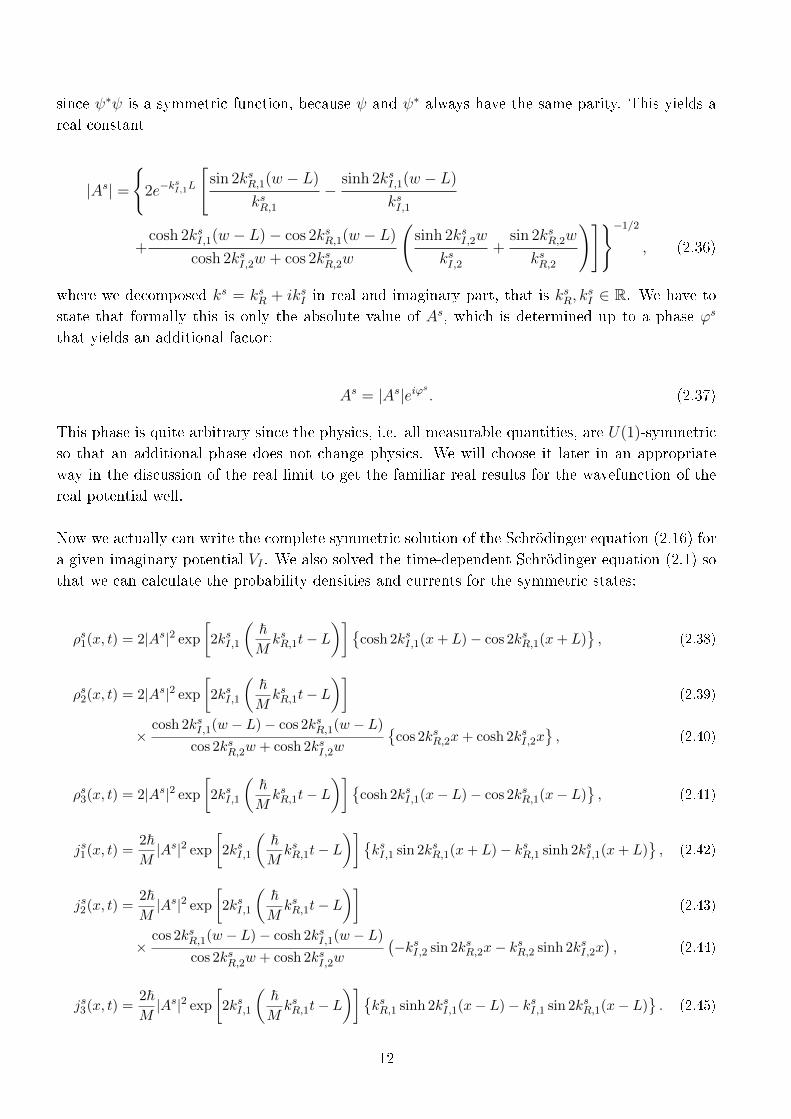
since ψ∗ψ is a symmetric function, because ψ and ψ∗ always have the same parity. This yields a
real constant
|As| =
{2e−k
sI,1L
[sin 2ksR,1(w − L)
ksR,1−
sinh 2ksI,1(w − L)
ksI,1
+cosh 2ksI,1(w − L)− cos 2ksR,1(w − L)
cosh 2ksI,2w + cos 2ksR,2w
(sinh 2ksI,2w
ksI,2+
sin 2ksR,2w
ksR,2
)]}−1/2, (2.36)
where we decomposed ks = ksR + iksI in real and imaginary part, that is ksR, ksI ∈ R. We have to
state that formally this is only the absolute value of As, which is determined up to a phase ϕs
that yields an additional factor:
As = |As|eiϕs . (2.37)
This phase is quite arbitrary since the physics, i.e. all measurable quantities, are U(1)-symmetric
so that an additional phase does not change physics. We will choose it later in an appropriate
way in the discussion of the real limit to get the familiar real results for the wavefunction of the
real potential well.
Now we actually can write the complete symmetric solution of the Schrödinger equation (2.16) for
a given imaginary potential VI . We also solved the time-dependent Schrödinger equation (2.1) so
that we can calculate the probability densities and currents for the symmetric states:
ρs1(x, t) = 2|As|2 exp[2ksI,1
(~MksR,1t− L
)]{cosh 2ksI,1(x+ L)− cos 2ksR,1(x+ L)
}, (2.38)
ρs2(x, t) = 2|As|2 exp[2ksI,1
(~MksR,1t− L
)](2.39)
×cosh 2ksI,1(w − L)− cos 2ksR,1(w − L)
cos 2ksR,2w + cosh 2ksI,2w
{cos 2ksR,2x+ cosh 2ksI,2x
}, (2.40)
ρs3(x, t) = 2|As|2 exp[2ksI,1
(~MksR,1t− L
)]{cosh 2ksI,1(x− L)− cos 2ksR,1(x− L)
}, (2.41)
js1(x, t) =2~M|As|2 exp
[2ksI,1
(~MksR,1t− L
)]{ksI,1 sin 2k
sR,1(x+ L)− ksR,1 sinh 2ksI,1(x+ L)
}, (2.42)
js2(x, t) =2~M|As|2 exp
[2ksI,1
(~MksR,1t− L
)](2.43)
×cos 2ksR,1(w − L)− cosh 2ksI,1(w − L)
cos 2ksR,2w + cosh 2ksI,2w
(−ksI,2 sin 2ksR,2x− ksR,2 sinh 2ksI,2x
), (2.44)
js3(x, t) =2~M|As|2 exp
[2ksI,1
(~MksR,1t− L
)]{ksR,1 sinh 2k
sI,1(x− L)− ksI,1 sin 2ksR,1(x− L)
}. (2.45)
12

We can con�rm that ρs(x, t) is a symmetric function while js(x, t, ) is antisymmetric, since
obviously ρs1(x, t) = ρs3(−x, t) and ρs2(x, t) = ρs2(−x, t) as well as js1(x, t) = −js3(−x, t) and
js2(x, t) = −js2(−x, t) is full�lled. The continuity of ρs can also directly be seen. One will also
be assured by evaluating ρs and js at x = ±w that the quantization condition (2.34), which has
to be full�lled by ks1 and ks2, provides di�erentiability of ρs and continuity of js right there. The
discussion of the continuity equation has already shown that js is not di�erentiable at that points.
We can now compute the continuity equation for the three areas and verify that (2.15) is valid,
since according to Eq. (2.21) it is ksR,1ksI,1 = M
~2EsI and k
sR,2k
sI,2 = M
~2 (EsI + C) and thus
∂
∂tρs(x, t) +
∂
∂xjs(x, t) =
{2~Mρs2(x, t)
(ksR,1k
sI,1 − ksR,2ksI,2
)= −2C
~ ρs2(x, t), |x| < w
0, otherwise
=2
~VI(x)ρs(x, t). (2.46)
That corresponds, indeed, exactly to the general continuity equation (2.15).
2.4.1 Real limit
Next we check these results for consistency by evaluating them in the limit C −→ 0, the so called
real limit, with the aim to get the familiar solutions for E and ψ of the ordinary real potential
well.
For C = 0 we can directly deduce from (2.21) that ks1 = ks2 =: ks and so the quantization condition
(2.34) becomes:
ks tan (ksw) = −ks cot [ks(w − L)] ⇔ sin (ksw)
cos (ksw)+
cos [ks(w − L)]
sin [ks(w − L)]= 0
⇔ cos(ksw) cos[ks(w − L)] + sin(ksw) sin[ks(w − L)] = 0
⇔ cos(ksL) = 0. (2.47)
If we decompose this into real and imaginary part
cos ksL = cos (ksRL) cosh (ksRL)− i sin (ksRL) sinh (ksRL) = 0, (2.48)
we can extract two independent conditions for ksR and ksI . Since coshx does not have any real
root as well as cosx and sinx do not have any mutual root, these conditions have the quite short
form:
cos ksRL = 0 and sinh ksIL = 0. (2.49)
Here sinhx only vanishes if and only if x = 0. Since L 6= 0 in general we can conclude that ksI = 0
and therefore ks is a real number. Using this we can conclude directly from (2.21) that also the
energy Es becomes real, that is EsI = 0. The condition cos ksRL = 0 yields
13

ksR = ksn =π
2L(2n+ 1) ⇒ Es = Es
n =~2
2M(ksn)2 =
~2π2
8ML2(2n+ 1)2, (2.50)
which are the energies of the symmetric states of the real potential well for integer n. Next we
evaluate the normalization constant for vanishing perturbation. Therefore, we look at Eq. (2.36)
and set ksI,1 = ksI,2 = 0 and ksR,1 = ksR,2 = π2L
(2n+ 1) = ks. With the help of De L'Hospital we get
limx→0
sinh ax
x= a (2.51)
as well as cos 2ks(w − L) = − cos 2ksw and sin 2ks(w − L) = − sin 2ksw, so we can directly derive
the result
|As0| ={
2
[−sin 2ksw
ks− 2(w − L) + 2w +
sin 2ksw
ks
]}−1/2=
1
2√L. (2.52)
Finally we check the wavefunction in the unperturbed case. Therefore, we formally distinguish
between ψs1,0 and ψs2,0 and we will see that the width w drops out so that we end up with ψs1,0 = ψs2,0.
Formally we have to insert As = 12√Leiϕ
sinstead of (2.52) since we only determined the absolute
value of the normalization constant so that an arbitrary phase ϕs additionally occurs. Before
inserting all that into the wavefunctions we �rst give the results of some direct calculations from
the value of the unperturbed wave number ks which will make the following computations clearer:
e±iksnL = ±iξn , sin ksn(x± L) = ±ξn cos ksnx , cos ksn(x± L) = ∓ξn sin ksnx, (2.53)
where we have introduced
ξn :=
{−1 , n is odd
+1 , n is even. (2.54)
If we insert ks into the symmetric wavefunction in area 1 from (2.31) and 2 from (2.33) and make
use of these identities, it is quite straight forward to derive the desired result, where we note that
ξ2n = 1 for every n:
ψs1,0(x) = −2i1
2√Leiϕ
s · iξn · ξn cos ksnx = eiϕs 1√
Lcos ksnx , (2.55)
ψs2,0(x) = 2i1
2√Leiϕ
s · iξn−ξn cos ksnw
cos ksnwcos ksnx = eiϕ
s 1√L
cos ksnx, (2.56)
which is indeed the same. Because of the symmetry of the cosine function, the condition ψs1(x) =
ψs3(−x) is automatically full�lled so that the barrier at x = ±w generally vanishes and thus we
can describe the whole wavefunction inside the potential well by one single expression:
14

ψs0(x) = eiϕs 1√
Lcos ksnx. (2.57)
By comparing this with the familiar result
ψs0(x) =1√L
cos ksnx, (2.58)
we can conclude that an appropriate choice for the phase would be ϕs = 0. Thus the normalization
constant As is real, that is
As = |As| . (2.59)
Now we check the validity of the continuity equation in the case of a real potential. At �rst we can
state that for all three areas the right-hand side of (2.46) has to vanish and according to Eq. (2.9)
also the time derivative of the density is equal to zero since EsI = 0. We can conclude this also
from the fact that H is hermitian in the real case, therefore U is an unitary operator and thus
ρs(x, t) is static and reads
ρs0(x, t) = U(t, t0)U†(t, t0)︸ ︷︷ ︸
=1
ρs0(x, t0) = ρs0(x, t0) = 4 |As0|2 cos2 ksx =
1
Lcos2 ksx, (2.60)
which can be also derived from (2.38) � (2.41). Therefore, we have to show for consistency that∂∂xjs0(x, t) = 0. A direct calculation yields from (2.42) � (2.44) that even js0 ≡ 0, since ksI = 0 in
the unperturbed case.
2.4.2 Limit of vanishing waist
Finally we check what happens if the perturbation vanishes when the width of area 2 goes to zero.
This should have the same e�ect as evaluating the system for C → 0, i.e. the real limit. We can
con�rm that this, indeed, comes out of the calculation. We only have to check this for Eq. (2.34)
knowing that this is the right background for all results we got for the real limit:
limw→0
ks2 tan (ks2w)︸ ︷︷ ︸→0
+ks1 cot [ks1(w − L)]
= ks1cos ks1L
sin ks1L= 0. (2.61)
We can see that ks2 drops out which is plausible. We neglect the uninteresting case ks1 = 0 but
state that ks1 has to full�ll cos ks1L = 0 and thus must be real for the same reasons as in the real
limit. Therefore, we call ks := ks1 the wavenumber for the whole interval [−L,L], which are area
1 and 3 for vanishing w, and obtain the same results as we got for the real limit.
15

2.5 Antisymmetric states
Now we evaluate the antisymmetric states of the complex potential well. From Section 2.3 we can
deduce the following antisymmetric wavefunctions in area 1 � 3:
ψa1(x) = −2iAaeika1L sin [ka1(x+ L)] , (2.62)
ψa2(x) = −2iAa ·Ra sin (ka2x) = −2iAaeika1L
sin [ka1(w − L)]
sin (ka2w)sin(ka2x) , (2.63)
ψa3(x) = −2iAaeika1L sin [ka1(x− L)] . (2.64)
With these expressions for the antisymmetric wavefunction we can implement the di�erentiability
at x = −w and thus get the quantization condition of the antisymmetric states:
∂ψa1∂x
∣∣∣∣x=−w
=∂ψa2∂x
∣∣∣∣x=−w
⇔ −ka1 cos [ka1(w − L)] = −ka2sin [ka1(w − L)]
sin (ka2w)cos(ka2w)
⇔ ka1 cot [ka1(w − L)]− ka2 cot (ka2w) = 0. (2.65)
Just like in the symmetric case we end up with a transcendental equation that determines ka1 and
ka2 , which can in general not be solved algebraically. Now we calculate the normalization constant
Aa of the antisymmetric states just like we did for the symmetric ones and get:
|Aa| =
{2e−2k
aI,1L
[sin 2kaR,1(w − L)
kaR,2−
sinh 2kaI,1(w − L)
kaI,2
+cos 2kaR,1(w − L)− cosh 2kaI,1(w − L)
cos 2kaR,2w − cosh 2kaI,2w
(sinh 2kaI,2w
kaI,2−
sin 2kaR,2w
kaR,2
)]}−1/2. (2.66)
Just as for the symmetric states we formally have to consider an additional phase to get Aa out
of |Aa|:
Aa = |Aa| eiϕa . (2.67)
An appropriate choice will be provided by the discussion of the real limit.
Now let us compute the probability density ρa(x, t) and the probability current ja(x, t) for the
antisymmetric states:
16

ρa1(x, t) = 2|Aa|2 exp[2kaI,1
(~MkaR,1t− L
)]{cosh 2kaI,1(x+ L)− cos 2kaI,1(x+ L)
}, (2.68)
ρa2(x, t) = 2|Aa|2 exp[2kaI,1
(~MkaR,1t− L
)](2.69)
×cos 2kaR,1(w − L)− cosh 2kaI,1(w − L)
cos 2kaR,2w − cosh 2kaI,2w
{cosh 2kaI,2x− cos 2kaR,2x
}, (2.70)
ρa3(x, t) = 2|Aa|2 exp[2kaI,1
(~MkaR,1t− L
)]{cosh 2kaI,1(x− L)− cos 2kaI,1(x− L)
}, (2.71)
ja1 (x, t) =2~M|Aa|2 exp
[2kaI,1
(~MkaR,1t− L
)]{kaI,1 sin 2k
aR,1(x+ L)− kaR,1 sinh 2kaI,1(x+ L)
}, (2.72)
ja2 (x, t) =2~M|Aa|2 exp
[2kaI,1
(~MkaR,1t− L
)](2.73)
×cos 2kaR,1(w − L)− cosh 2kaI,1(w − L)
cos 2kaR,2w − cosh 2kaI,2w
(kaI,2 sin 2k
aR,2x− kaR,2 sinh 2kaI,2x
), (2.74)
ja3 (x, t) =2~M|Aa|2 exp
[2kaI,1
(~MkaR,1t− L
)]{kaI,1 sin 2k
aR,1(x− L)− kaR,1 sinh 2kaI,1(x− L)
}. (2.75)
We can state the same results concerning symmetry of ρa and antisymmetry of ja as for the
symmetric states. A small calculation would show that the quantization condition (2.34), which
ka1 and ka2 have to full�ll, ensures that ρa is di�erentiable and ja is continuous at x = ±w. We
already found out that ja could not be di�erentiable right there.
We can now evaluate the continuity equation for the antisymmetric states and verify that (2.15)
is valid also for them, since according to Eq. (2.21) it is kaR,1kaI,1 = M
~2EaI and k
aR,2k
aI,2 = M
~2 (EaI +C)
and thus
∂
∂tρa(x, t) +
∂
∂xja(x, t) =
{2~Mρa2(x, t)
(kaR,1k
aI,1 − kaR,2kaI,2
)= −2C
~ ρa2(x, t), |x| < w
0, otherwise
=2
~VI(x)ρa2(x, t). (2.76)
That corresponds indeed exactly to the general continuity equation (2.15). Therefore, the conti-
nuity equation holds for states with both parities.
2.5.1 Real limit
Now we evaluate the antisymmetric states for C → 0 and proceed just like we did for the symmetric
states. First we deduce from (2.21) that ka1 = ka2 = ka so that we can solve (2.65) analytically:
ka cot ka(w − L)− ka cot kaw = 0 ⇔ 0 = cos[ka(w − L)] sin(kaw)− cos(kaw) sin[ka(w − L)]
⇔ 0 = sin kaL. (2.77)
Decomposing ka into real and imaginary part provides
17

sin kaL = cosh(kaIL) sin(kaRL) + i sinh(kaIL) cos(kaRL) = 0, (2.78)
from which we extract the following two equations
sin(kaRL) = 0 and sinh(kaIL) = 0, (2.79)
since coshx has no real root as well as sinx and cosx have no mutual root. This provides that ka
is real just like in the symmetric case and has to full�ll
ka = kan =nπ
L⇒ Ea = Ea
n =~2π2
2ML2n2, (2.80)
which are exactly the results from the real potential well for integer n. The normalization constant
Aa becomes
|Aa| ={
2
[sin 2kaw
ka− 2(w − L) + 2w − sin 2kaw
ka
]}−1/2=
1
2√L, (2.81)
since (2.51) as well as sin 2kaR(w − L) = sin 2kaRw and cos 2kaR(w − L) = cos 2kaRw for kaR = nπL
and kaI = 0. Now we ensure that the wavefunction, which is separated into 3 parts, turns into the
familiar form
ψan(x) =1√L
sin kanx. (2.82)
Therefore, we use some identities which directly follow from kan = nπL:
e±ikanL = ξn , sin kan(x± L) = ξn sin kanx , cos kan(x± L) = ξn cos kanx, (2.83)
with ξn de�ned in (2.54). So the antisymmetric wavefunction in area 1 and 2 reads:
ψa1(x) = −2ieiϕa 1
2√Lξn · ξn sin kanx = −ieiϕa 1√
Lsin kanx , (2.84)
ψa2(x) = −2ieiϕa 1
2√Lξnξn sin kanw
sin kanwsin kanx = −ieiϕa 1√
Lsin kanx, (2.85)
since ξ2n = 1. The wavefunction in area 3 is determined by ψa1(x) and due to the antisymmetry
of the sine function we can deduce that ψa1 = ψa2 = ψa3 in the real case which we denote with ψa0 .
In the end we clarify the phase ϕa by comparing our result with the solutions (2.82) of the real
potential well. Thus we have to choose ϕa so that −ieiϕa = 1, that is ϕa = π/2. Therefore, the
normalization constant is completely imaginary:
18
Aa = i |Aa| . (2.86)
Finally we evaluate the continuity equation in the real limit, which is quite the same discussion
as for the symmetric states. For the same reason the time evolution operator U is unitary for a
vanishing imaginary potential. Therefore, the density looses its time dependence:
ρa0(x, t) = U(t, t0)U†(t, t0)︸ ︷︷ ︸
=1
ρa0(x, t0) = ρa0(x, t0) = 4 |As0|2 sin2 kax =
1
Lsin2 kax, (2.87)
so that its derivative with respect to t is equal to zero. A direct calculation shows from (2.72) �
(2.75) that ja0 ≡ 0 so that the continuity equation in the real limit is full�lled since both terms
vanish.
2.5.2 Limit of vanishing waist
We can derive this result also by evaluating w → 0 along the same line as for the symmetric states.
We only have to make a slight transformation of Eq. (2.65), that is equivalent to
ka2 tan ka1(w − L)− ka1 tan ka2w = 0. (2.88)
Thus, we can immediately evaluate this expression for w → 0:
limw→0
ka2 tan [ka1(w − L)]− ka1 tan (ka2w)︸ ︷︷ ︸→0
= ka2sin ka1L
cos ka1L= 0. (2.89)
One sees that ka2 drops out again since ka2 6= 0 and so the new condition is now sin ka1L = 0. This
is indeed the same condition as for the real limit so that we can call ka1 = ka and adopt completely
its results to the limit of vanishing waist.
19

3 Numerical analysis
Both quantization conditions (2.34) and (2.65) are transcendental equations and are, therefore,
not solvable in an algebraic way. Thus, we have to �nd its solutions k1 = k1(C) and k2 = k2(C)
numerically. Both variables depend on the energy E = E(C) so that we can rewrite (2.34) and
(2.65) in terms of the energy to have an equation only depending on one variable, which is more
comfortable to solve.
3.1 Some further theoretical discussion
Before starting with the numerical calculation it is useful to have some further theoretical in-
sights of the so far derived formulas. This will make it easier to have an appropriate physical
interpretation of the numerical results afterwards.
3.1.1 Dimensionless variables
First of all we express all variables in a dimensionless way. Therefore, we use from now on the
following dimensionless quantities:
ε :=E
~22M
(π2L
)2 , c :=C
~22M
(π2L
)2 , κ :=kπ2L
, χ :=x2Lπ
, ω :=w2Lπ
. (3.1)
In terms of these new variables the quantization conditions (2.34) and (2.65) now read
0 = κs1 cot[κs1
(ω − π
2
)]+ κs2 tan (κs2ω) , (3.2)
0 = κa1 cot[κa1
(ω − π
2
)]− κa2 cot (κa2ω) . (3.3)
If we reexpress (2.21) in terms of the new variables
κ1 =√ε and κ2 =
√ε+ ic, (3.4)
we can rewrite (3.2) and (3.3) for a given dimensionless waist ω as a function of only one complex
quantity ε = ε(c):
0 =√εs cot
[(ω − π
2
)√εs]
+√εs + ic tan
(ω√εs + ic
), (3.5)
0 =√εa cot
[(ω − π
2
)√εa]−√εa + ic cot
(ω√εa + ic
). (3.6)
The symmetric wavefunctions (2.31) � (2.33) now read:
20

ψs1(χ) = −2iAeiκs1π2 sinκs1
(χ+
π
2
), (3.7)
ψs2(χ) = 2iAeiκs1π2
sinκs1(ω − π
2
)cosκs2ω
cosκs2χ , (3.8)
ψs3(χ) = ψs1(−χ) = 2iAeiκs1π2 sinκs1
(χ− π
2
), (3.9)
whereas the antisymmetric ones (2.62) � (2.64) reduce to
ψa1(χ) = −2iAeiκa1π2 sinκa1
(χ+
π
2
), (3.10)
ψa2(χ) = −2iAeiκa1π2
sinκa1(ω − π
2
)sinκa2ω
sinκa2χ , (3.11)
ψa3(χ) = −ψa1(−χ) = −2iAeiκa1π2 sinκa1
(χ− π
2
). (3.12)
Since the normalization constant A has still the dimension 1/√L, the densities ρ (χ) = ψ (χ)∗ ψ (χ)
scale with 1/L as it should be.
3.1.2 Limit of big waist
It will turn out to be quite useful to have some initial theoretical discussion of (3.5) and (3.6)
before solving them for several ω and c. We have already done the "limit of vanishing waist",
that is ω → 0, and got the familiar case of the real potential well, that is εI = 0. We can consider
this as a kind of simple limit case for the potential well getting real again. However, we did not
yet evaluate the other extreme case w → L, that is ω → π2. Therefore, we consider Eqs. (3.2) and
(3.3) again and calculate this limit. We start with (3.2) and have to change it a bit:
0 = limω→π/2
κs1 cos[κs1
(ω − π
2
)]︸ ︷︷ ︸
→1
cos (κs2ω) + κs2 sin (κs2ω) sin[κs1
(ω − π
2
)]︸ ︷︷ ︸
→0
0 = cos
(κs2π
2
), (3.13)
since κs1 6= 0. With the same argumentation as in the real limit this could only be full�lled if and
only if κs2 is a real number, more precisely an odd integer one, that is κs2 = 2n + 1 where n is an
integer number. With (3.4) this means
κs2 =√εsR + i(εsI + c)
!= 2n+ 1 ∈ Z ⇒ εsI = −c, εsR = (2n+ 1)2. (3.14)
For the antisymmetric states we get the same result. If we change (3.3) a bit we get:
21

0 = limω→π/2
κa1 cos[κa1
(ω − π
2
)]︸ ︷︷ ︸
→1
sin (κa2ω)− κa2 cos (κa2ω) sin[κa1
(ω − π
2
)]︸ ︷︷ ︸
→0
0 = sin
(κa2π
2
). (3.15)
This is also a result which is full�lled by κa2 = 2n for integer n as we found out in Subsection 2.5.1.
Therefore, we can conclude from (3.4):
κa2 =√εaR + i(εaI + c)
!= 2n ∈ Z ⇒ εaI = −c, εaR = (2n)2, (3.16)
which is indeed the same result for εI .
Thus we can state that these two kinds of limits for the waist ω yield two di�erent conditions for
the imaginary part of the energy εI , that is
limω→0
εI = 0 and limω→π/2
εI = −c. (3.17)
It is an interesting fact that both limits of ω actually represent the real limit since we receive the
same wavenumbers for the nonvanishing area. Therefore, we will get the same wavefunctions as
in the real case. We will see in the evaluation of the numerical solutions that there is a quite
plausible reason for this observation.
3.2 Energies
3.2.1 Solutions
It is quite straight forward to �nd the roots of the left-hand side of (3.5) and (3.6) numerically
for given c and ω. In our dimensionless variables the energy of the symmetric states for vanishing
perturbation reads εR,n(0) = (2n+1)2 thus the symmetric ground state for the real potential well is
characterized by n = 0 in (2.50). For the antisymmetric states this condition reads εR,n(0) = (2n)2
and thus it seems to be comfortable to assign to every energy of a symmetric state the natural
number m := 2n+1 and to every antisymmetric state m := 2n. Therefore, all states denoted with
an odd m are symmetric while all states denoted with an even m are antisymmetric. Thus the
symmetric ground state is denoted by ε1, the �rst antisymmetric excited state by ε2 and so on.
We can conclude that every reasonable solution of (3.5) and (3.6) has now to full�ll εR,m(0) = m2
and εI,m(0) = 0 like we found out in the discussion of the real limit. This new assignment will
make it easier to do a general evaluation of all states in the potential well.
For increasing values of the dimensionsless waist ω we �nd the corresponding results shown in
Figs. 3 and 4:
22

Figure 3: Real and imaginary part of the lowest energy eigenvalues as a function of the strengthc of the imaginary potential for the waists ω = 0.2 − 0.7. Two curves with the same colourrepresent the real and imaginary part of the energy of the state, whereat the real part starts atεR(c = 0) = m2 and the imaginary part at εI(c = 0) = 0. Moreover, ε∞-states are counted byinteger n while ε0-states are counted by integer k.
23

Figure 4: Real and imaginary part of the lowest energy eigenvalues as a function of the strengthc of the imaginary potential for the waists ω = 0.8 − 1.1. Two curves with the same colourrepresent the real and imaginary part of the energy of the state, whereat the real part starts atεR(c = 0) = m2 and the imaginary part at εI(c = 0) = 0. Moreover, ε∞-states are counted byinteger n while ε0-states are counted by integer k.
It is interesting to see that one can generally divide all states into two groups. The states of the one
group, which we denote by ε∞, has a divergent imaginary part which goes for a large imaginary
potential linearly to in�nity, while the states of the other group have an imaginary part which
goes to zero for large c so that we denote them with ε0. Furthermore, every ε0�state approaches
to another ε0�state with the other parity so that we can observe pairs of one antisymmetric and
one symmetric ε0�state for c→∞ which tend to the same limit limc→∞ ε0.
For increasing imaginary potential of strength c the states behave more and more like in the case
of ω → 0 and ω → π/2. Moreover, one can state that for small ω there are more ε0�states
among the lowest 5 energy levels, while the number of ε∞�states increases for higher ω in that
group of states with lower energy. It seems that the assignment of a state to the group of ε∞�
or ε0�states strongly depends on the saturation value of the real part of its energy εR, while it
apparently does not depend on parity or the energy value the state is starting at for c = 0. There
24
seems to be no obvious rule for this classi�cation but a look at the numerical solutions for large
values c gives the impression that it has to do something with the order of the saturation values
of the �rst 5 states. If we neglect the behaviour for small c the real part of the energy of every
plotted state is monotonously increasing for large c and arrives at some �nite saturation value
as we can conclude from the numerical solutions. These values seem to depend on the waist ω
in a way that the saturation values of εR of ε∞�states are decreasing with ω while these of the
ε0�state are increasing with ω. Therefore, for increasing waists the lower energy levels become ε∞while the ε0�states are pushed to higher energy levels. In Figs. 3 and 4 we can observe that the
states starting at low energies of the real potential well, that is c = 0, for example the energies
of the states m = 1 or m = 2 of the real potential well, are ε0 for small waists like ω = 0.2 and
become ε∞ for large waists like ω = 1.1. Thus we can see that the essential order of the energies
is not seriously changed so that there has to be a kind of replacement of ε0 states by ε∞�states
for some critical values of ω. For ω = 0.3, 0.8, 1 one can observe an unusual development of the
two involved states which for lower c attract and from some c on reject each other. For increasing
c they are getting closer and closer at this speci�c c and then something remarkable happens.
At some critical waist ωcrit the "upper" state, which is a ε∞ one, is not rejected any more by
the lower ε0�state but changes roles with it. An intersection occurs and the state starting at the
lower energy, i.e. c = 0, now becomes the new ε∞ one and has the larger saturation value while
the former ε∞, which started at the higher level, now is ε0 and fuses with the opposite parity
state in between converging to the lower saturation value of the real part of the energy. We can
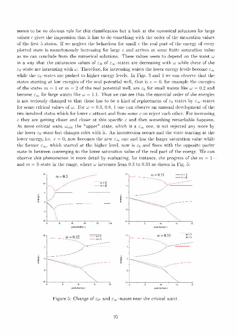
observe this phenomenon in more detail by evaluating, for instance, the progress of the m = 1�
and m = 3�state in the range, where ω increases from 0.3 to 0.33 as shown in Fig. 5:
Figure 5: Change of ε0- and ε∞�states near the critical waist.
25

It is not possible to determine the exact ωcrit graphically because it depends on the assignment of
particular solutions of (3.5) to the one or the other curve which seems to be quite arbitrary since
both possible curves do not change in a su�ciently traceable way. We have already found out that
the saturation value of the real part of ε0�states increases with c, while for ε∞�states it decreases
with c. Moreover, we know that also the particular assignment whether a state is ε0 or ε∞ has
something to do with its saturation value. The question of the exact ωcrit and the occurrence
of the intersection is thus an additional motivation to revisit the quantization conditions and to
calculate the saturation value of εR for c → ∞. This should be ω-dependent and contain some
kind of quantum number to enumerate the di�erent ε0� and ε∞�states, which we already called
k and n. This shall provide at least a condition for the intersection of two states which does
not change roles for larger waists ω. This property is important since otherwise one will not see
any indication for an intersection in the ε�ω�diagram because the ε∞�state stays the upper one
before and after ωcrit. In other words the ε-ω-diagram does not know any m which contains the
information where a state starts for c = 0. Another interesting issue that may be then explained
is the fusion of two states with di�erent parities that tend to the same energy limit.
At this point it seems to be reasonable to spend some time on calculating the repeatedly mentioned
saturation value of the real part of the energies.
3.2.2 Saturation value for real part of energy
Now we evaluate the saturation value of the real part of the energy εR from the transcendental
equations (3.5) and (3.6). We start with the symmetric one:
√εs cot
[(ω − π
2
)√εs]
+√εs + ic tan
[ω√εs + ic
]= 0. (3.18)
By inserting the two empirically known kinds εI,∞ and εI,0 of behaviour of the imaginary part εIfor c→∞, that is
limc→∞
εsI,∞ = − limc→∞
c and limc→∞
εsI,0 = 0, (3.19)
we are con�dent to get a corresponding result for the real part εsR. We start with ε∞. Inserting
εsI,∞ → −c into (3.5) provides
√εsR,∞ − ic cot
[(ω − π
2
)√εsR,∞ − ic
]+√εsR,∞ tan
[ω√εsR,∞
]= 0. (3.20)
Since εR ∈ R in any case the second term on the left-hand side is already real. Therefore, we split
up the �rst one. To do this we use the polar expression of complex numbers z = x+ iy
z = |z|eiφ =√x2 + y2ei arctan
yx , (3.21)
where x, y ∈ R. For the square root of complex numbers then follows directly:
√z =
√|z|e
i2φ =
(x2 + y2
)1/4ei2arctan y
x . (3.22)
26

We use this for the expression√εsR,∞ − ic in Eq. (3.20):
√εsR,∞ − ic =
[(εsR,∞
)2+ c2
]1/4exp
[− i
2arctan
c
εsR,∞
]. (3.23)
Since εsR,∞ tends to some �nite value, we can approximate the absolute value by[(εR,∞)2 + c2
]1/4 ≈√c and get for the phase
limc→∞
arctanc
εsR,∞= (2j + 1)
π
2, j ∈ Z. (3.24)
This yields the phase −π4(2j + 1), which leads to four formally distinct solutions:
√c exp
[−iπ
4(2j + 1)
]=
√c
2
1− i , j = 0, 4, 8, ...
−(1 + i) , j = 1, 5, 9, ...
−(1− i) , j = 2, 6, 10, ...
1 + i , j = 3, 7, 11, ...
. (3.25)
If we insert this into the �rst term of the left-hand side of (3.20), we can directly conclude that,
since cotangens is an odd function, always two solutions, which only di�er from each other by a
global minus sign, are equivalent in this case. Therefore, we only have to distinguish between the
cases√
c2(1 + i) and
√c2(1− i), that is between even and odd numbers j.
We start with odd j. Inserting√εsR,∞ + ic ≈
√c2(1 + i) into the �rst term on the left-hand side
of (3.20) provides
√c
2(1 + i) cot
[√c
2(1 + i)
(ω − π
2
)]=
√c
2(1 + i)
− sin[√
2c(ω − π
2
)]+ i sinh
[√2c(ω − π
2
)]cos[√
2c(ω − π
2
)]− cosh
[√2c(ω − π
2
)] . (3.26)
Since cosx ∈ [−1, 1] for all x ∈ R and limx→∞ coshx = ∞ we can neglect the cosine in the
denominator of (3.26). For the same reason we can replace (1+i)(− sinx+sinh x) by −(1−i) sinhx
for x→∞. These approximations provide
√c
2(1− i)
sinh[√
2c(ω − π
2
)]cosh
[√2c(ω − π
2
)]︸ ︷︷ ︸→1
≈√c
2(1− i). (3.27)
Therefore, we can approximate the �rst term on the left-hand side of (3.20) by the complex
expression√
c2(1 − i). The same calculation for even j yields a positive imaginary part, that is√
c2(1 + i). The resulting equation reads
√c
2(1± i) +
√εsR,∞ tan
[ω√εsR,∞
]= 0. (3.28)
27

For the saturation value of εsR,∞ we have to evaluate the real part of this equation which is the
same in both cases of j:
√c
2+√εsR,∞ tan
[ω√εsR,∞
]= 0. (3.29)
The �rst term tends obviously to in�nity which can only be compensated if the tangens has a
singularity at the saturation value. This means:
ω√εsR,∞ = (2n− 1)
π
2⇔ εs,nR,∞ = (2n− 1)2
π2
4ω2, n ∈ Z. (3.30)
For εs0 we get instead of (3.20):
√εsR,0 cot
[(ω − π
2
)√εsR,0
]+√εsR,0 + ic tan
[ω√εsR,0 + ic
]= 0. (3.31)
We can see that in this case the �rst term of the left-hand side is already real so let us �nd
the complex decomposition of the second term. We will do so with the same approach via polar
expression as we did for εs∞. Then we �nally end up with
√c
2(−1± i) +
√εsR,0 cot
[√εsR,0
(ω − π
2
)]= 0. (3.32)
One can see that only the real part contains εR. Therefore, we only evaluate this part of the
equation since the imaginary part does not provide anything reasonable so that the used approx-
imation seems not to be appropriate for it. The real part of this equation yields that cotangens
has to have a singularity at√εsR,0
(ω − π
2
). We can thus conclude:
√εsR,0
(ω − π
2
)= kπ ⇔ εs,kR,0 =
k2π2(ω − π
2
)2 , k ∈ Z. (3.33)
The same calculations for the antisymmetric states and their quantization condition
√εa cot
[√εa(ω − π
2
)]−√εa + ic cot
(ω√εa + ic
)= 0 (3.34)
yields the following saturation values for εaR:
εa,nR,∞ =n2π2
ω2and εa,kR,0 =
k2π2(ω − π
2
)2 . (3.35)
Note that we used for consistency k and n and de�ned them in a way that both are starting at
1. Furthermore, we notice the remarkable result that εs,kR,0 = εa,kR,0 for each value of k which can be
proved by inspecting the respective graphs. This corresponds to the observation that always two
28

ε0�states with di�erent parities are becoming one state for c→∞.
It may clarify to ignore the particular parity of the saturation values, since it obviously does not
matter for the ε0�states. Thus we can write for convenience
εnR,∞ =n2π2
4ω2and εkR,0 =
k2π2(ω − π
2
)2 (3.36)
and note for εnR,∞ that even n are standing for antisymmetric states and odd n for symmetric
ones.
3.2.3 Discussion
We can read o� from (3.36) an interesting connection to the energies of a real potential well which
con�rms our suggestion from Subsection 3.1.2 that for c → ∞ an e�ective potential well within
±ω occurs. If we take the original variables instead of the dimensionless ones this will be obvious.
From (3.36) we read o� at �rst
EnR,∞ =
~2
2M
π2
4L2
n2π2
4
4L2
π2w2=
~2π2
8Mw2n2. (3.37)
Comparing this result with the energies of the real potential well (2.50) and (2.80), we conclude
that we received the energy of a potential well with the width 2w where we note that symmetric
and antisymmetric states are included in this formula. Similarly we get for the other formula
EnR,0 =
~2
2M
π2
4L2
n2π2
4
4L2
π2(w − L)2=
~2π2
8M(L− w)2n2, (3.38)
which are the energies of a potential well with the width L − w that is the outer region of the
waist. This insight and the good accordance to the numerical solutions ensures us that we found
serious and plausible formulas to calculate the real part of the energy in the limit c→∞.
By taking a look at the results graphically in Fig. 6, one can see that the convention to mix up
symmetric and antisymmetric states is quite reasonable, since the parity of the corresponding
state does not matter and we count all energies of one type by only one integer number.
29

Figure 6: Saturation values of the real part of the energy εR(ω) for ε0�states counted by k andε∞�states counted by n.
The intersections in Fig. 6 con�rm the occuring intersections of the particular states in Figs. 3
and 4. Like we suspected it is only possible to calculate the intersection of two states if they keep
their character. This is always full�lled if the involved ε∞�state is �rst the upper one so that
after the corresponding critical value the saturation value of the corresponding ε0�state is higher.
This process can be directly seen from the derived formulas (3.36) since ε0 is strictly monotonic
decreasing while ε∞ is strictly monotonic increasing in the considered interval ω ∈ [0, π/2]. As
we already argued these formulas unfortunately do not provide any new information about the
occurring process running vice verca with a change of the behaviour of both involved states after
it. However it catches the eye that each one of these processes occurs for nearly the same ω where
a process of the other kind appears. Since we have already argued that there can not be any strict
rule to determine ωcrit we have to make an agreement for which ω the change precisely occurs.
Let us thus connect this value to the corresponding intersection in Fig. 6 so that the 3 values of
ωcrit we can read o� from Figs. 3 and 4 are π/10, π/4 and π/3. The intersection at ω = π/3 does
not occur in Fig. 6 because the corresponding states are for example ε1R,∞ and ε4R,0 which are not
plotted together in this graph.
Finally, let us discuss boundaries of the considered interval of ω. We know that εI = 0 for ω → 0.
Therefore, we only evaluate ε0 for this boundary since obviously limω→0 εR,∞ = ∞. As we have
already seen in the Subsections 2.4.2 and 2.5.2 this should provide the real limit, that is εR = k2.
Unfortunately (3.36) yields
limω→0
εkR,0 = 4k2 . (3.39)
This looks inconsistent but actually it is not since the approximation we used does not hold for
30

ω = 0 because the area, where the imaginary potential acts at, vanishes. Therefore, the resulting
formula does not have any reference to the problem since the approximation is based on c � εRwhich does not make any sense if c is not involved in the problem any more.
This argumentation is supported by the fact that the evaluation of the other boundary ω → π/2
provides the correct result. As we know from Subsection 2.5.2 the considered energies are ε∞ as
we can also see from the corresponding formula that yields limω→π/2 εR,0 = ∞. Taking the limit
of the other one leads to:
limω→π/2
εnR,∞ = n2. (3.40)
These are the dimensionless energies of the real potential well which should occur for ω → π/2 as
we found out in Subsection 3.1.2.
All in all we can state that in the case of a pure potential well, whereat it does not matter whether
it is real or imaginary as we have seen in Subsection 3.1.2, there occurs only one kind of energies
that we called ε0 and ε∞. In the case of 0 < ω < π/2, that is two nested potential wells, these
kinds of states are mixed. That means that both types are occurring simultaneously. However one
can observe and calculate from (3.36) that for small waists there are more ε0�states appearing for
low energies since ε∞ is really high for small waists while for ω → π/2 the ε0�states are vanishing
from our focus because their energy goes to in�nity and the ε∞�states take their place as the
energies of the emerging potential well. This trend is quite obvious from the development of the
energy states with ω one can observe from Figs. 3 and 4.
3.3 Densities
3.3.1 Solutions
With (3.5) and (3.6) we can directly calculate from ε(c) numerical solutions for the dimensionless
wavenumbers κ1(c) and κ2(c) via (3.4) and (3.22):
κ1 =[ε2R + ε2I
]1/4cos
(1
2arctan
εIεR
)+ i[ε2R + ε2I
]1/4sin
(1
2arctan
εIεR
), (3.41)
κ2 =[ε2R + (εI + c)2
]1/4cos
(1
2arctan
εI + c
εR
)+ i[ε2R + (εI + c)2
]1/4sin
(1
2arctan
εI + c
εR
). (3.42)
Thus it is possible to evaluate the corresponding wavefunctions ψ(χ) and densities ρ(χ) for the
diverse behaviour of ε(c) we have so far studied. Nevertheless it seems to be quite tedious to
evaluate all densities for every waist, perturbation and energy. Therefore, it will turn out to be
su�cient to evaluate only some selected examples to bring out the main statement. That means
we plot the densities of some ε0- and ε∞�states and discuss them. Note that now it makes sense
to distinguish between symmetric and antisymmetric states since it will turn out to be interesting
how the parity of the state evolves with c. Therefore, since ε0�states are counted by k and ε∞�
states by n, the parity of εn∞ is given by n, that is symmetric if n is odd and antisymmetric if n is
even. The parity of εk0 is given by k in a similar way. Moreover, we used dimensionless densities,
that means to get the correct dimension we have to multiply each result with 2π/L.
31

Figure 7: Densities of the lowest energies for ω = 0.3 for some values of c, where all states arecounted by m for c = 0 and by k if they are ε0 and by n if they are ε∞ for c → ∞. Thefusion of respectively two ε0-states, which we already observed in Figs. 3 and 4, is con�rmed here.Furthermore, it shows that two states with the same k end up exactly in the same state.
32

Figure 8: Densities of the lowest energies for ω = 0.4 for some values of c, where all states arecounted by m for c = 0 and by k if they are ε0 and by n if they are ε∞ for c → ∞. Thefusion of respectively two ε0-states, which we already observed in Figs. 3 and 4, is con�rmed here.Furthermore, it shows that two states with the same k end up exactly in the same state.
33

Figure 9: Densities of the lowest energies for ω = 0.6 for some values of c, where all states arecounted by m for c = 0 and by k if they are ε0 and by n if they are ε∞ for c → ∞. Thefusion of respectively two ε0-states, which we already observed in Figs. 3 and 4, is con�rmed here.Furthermore, it shows that two states with the same k end up exactly in the same state.
34

Figure 10: Densities of the lowest energies for ω = 0.8 for some values of c, where all statesare counted by m for c = 0 and by k if they are ε0 and by n if they are ε∞ for c → ∞. Thefusion of respectively two ε0-states, which we already observed in Figs. 3 and 4, is con�rmed here.Furthermore, it shows that two states with the same k end up exactly in the same state.
35

Figure 11: Densities of the lowest energies for ω = 1.1 for some values of c, where all statesare counted by m for c = 0 and by k if they are ε0 and by n if they are ε∞ for c → ∞. Thefusion of respectively two ε0-states, which we already observed in Figs. 3 and 4, is con�rmed here.Furthermore, it shows that two states with the same k end up exactly in the same state.
36

3.3.2 Discussion
Figs. 7 � 11 allow a very deep insight in what is really happening with the energies and states
in this nested complex potential well. We already found out that in the case of vanishing waist
ω → 0 the imaginary part of the energy vanishes, too, that is εI = 0. Thus we are left with
only ε0�states, which are the familiar states of the real potential well, because the energy of the
ε∞�states tends to in�nity. If we take the opposite case of ω → π/2 then only ε∞�states are
remaining, because in this case the energy of ε0�states diverges. In contrast to ε0�states they are
complex which yields an imaginary part of the energy that corresponds exactly to the strength of
the perturbation or rather the depth of the imaginary potential well, that is εI = −c. Therefore,we can conclude that the ε0�states are these of the real potential well as we already found out in
the discussion of the real limit, while the ε∞�states are the states of the imaginary potential well
with the depth c, which is also con�rmed by (3.37) and (3.38). They are quite the same states
and energies, as we found out in the discussion of the energy, with only one di�erence. There is an
imaginary part of the energy which yields the depth of the imaginary well. This could be already
concluded from the discussion of the energy.
Now let us have a concreter look at the densities. One can directly observe the distinct behaviour
of ε0�states, which are denoted by the integer number k, and ε∞�states, which are denoted by
the integer number n. A general tendency is that the maxima of probability are shifted in a quite
logical way. The maxima of ε0�states tend to area 1 and 3, while ε∞�states have maxima in area
2. The probability in the respective outer region, that is area 1 and 3 for ε∞ and area 2 for ε0,
decreases rapidly for increasing perturbation. A logical consequence of this is that the symmetric
ε0�states are vanishing because a maximum in the center of the well would be a contradiction to
this general development. Therefore, the only possible ε0�states are antisymmetric which have a
vanishing probability in the center of the well. For increasing c the maxima are displaced to the
borders of the well while in the inner region of the waist the probability decreases. Thus it looks
plausible that the symmetric states approach the nearest respective antisymmetric state and are
absorbed by it as we found out in the discussion in Section 3.2. This explains the fusion of each
pair of one symmetric and one antisymmetric we have already seen in Figs. 3 and 4. The result
is one antisymmetric state, whose probability maxima get out of the waist�region, and thus its
energy increases with ω.
The ε∞�states behave vice verca. For ω → 0 they can not occur because their energy tends to
in�nity. Because the imaginary potential well is in the center we can observe also symmetric
states. The probability in area 1 and 3 decreases for increasing c while the probability maxima
are shifted into the waist-region |χ| < ω. Thus for increasing perturbation a new completely
imaginary potential well emerges in the center of the whole potential well with symmetric and
antisymmetric states and a rapidly decreasing probability in the outside which is equal to zero for
c→∞. One could also interpret that, for very large c, the potential well is divided twice so that
every area is itself a potential well with symmetric and antisymmetric states.
One interesting issue is the shifting of the maxima in the respective region. This could be well
seen in Fig. 10 of the m = 2�state with ω = 0.8, which is ε∞, so that the density maxima tend
into the center. For c = 0 this is an antisymmetric state with two maxima which does not change
with perturbation. But we can observe that the maxima become more narrow and in the end are
also displaced. The interesting fact is that �rst they become a bit broader and smaller and for one
37

speci�c c the actual development to the �nal result starts. A closer look at this state in the energy
diagram (Fig. 3) shows us that there happens something interesting for c ∈ [10, 20]. Therefore,
let us have a closer look at this particular state for these values of perturbation:
Figure 12: Shifting of the maxima of m = 2�state for ω = 0.8 for c ∈ [10, 20]. Both maxima aredivided into two parts in the waist region. The parts in area 2 increase and become more narrowpeaks while the parts in area 1 and 3 decrease to zero.
In Fig. 12 one can see that the maximum divides into 2 parts since the border between area 1 and
2, that is |χ| = ω, runs nearly through the middle of the peak. The slightly bigger part is in area
2 so that this part grows while the other one reduces with increasing c so that in the end there
remains a narrow peak inside of area 2 and a decay to zero outside.
3.3.3 Critical waists
We have already seen that for c → ∞ the potential well is divided and each area becomes a
new real (area 1 and 3) or imaginary (area 2) potential well. So at the end we are left with
3 independent potential wells. The states of the former single real potential well for c = 0 are
divided up into the 3 new wells where we can genereally distinguish between states shifted to the
inside, that is area 2, whose imaginary part of the energy tends to −∞ and states shifted to the
outside, that is area 1 and 3, whose imaginary part vanishes for c→∞. The special assignment
38

of the states into these two groups depends obviously on the waist and at "critical waists" this
assignment is changed. Unfortunately we did not �nd out a rule for the occurrence of such critical
waists. We have rather argued in Subsection 3.2.1 that there is no compulsory rule that tells us
when the assignment exactly changes since we only work with single numerical values instead of
analyzable functions. In the discussion of Fig. 6 in Subsection 3.2.3 we have found out that the
calculated intersections, which unfortunately have nothing to do with the change of the assignment
into ε0 and ε∞, are though very near to waists where one can observe such a change of assignment.
Therefore, the only "rule" we have postulated so far is that each change of assignment emerges
precisely at the value of a waist where such an intersection occurs.
In the case of the antisymmetric �rst excited m = 2�state for ω = 0.8, that we have just disussed,
it seems to be quite obvious to determine a critical waist from this discussion. This case is insofar
special as this state remains a �rst excited state for c → ∞ namely of the imaginary potential
well in area 2. For the argumentation it is important that the state keeps its particular form, that
is it remains antisymmetric with two maxima. Let us take a look at Fig. 10 at the states m = 2
and m = 4. In both cases there is a little bit more area within the waist so that it should take less
energy to reduce the outer part of the peak as well as more energy to reduce the inner part and
get a narrow peak in the outer region. If we consult the corresponding energy diagram in Fig. 4
we can see that these states are special ones because their energies are very close and we know
from our discussion of the energy by comparing with ω = 0.7 that the red and the green curve just
have changed roles. That means that for ω = 0.7 the εn=2∞ �state has more energy and the εk=1
0
less while the situation is vice verca for ω = 0.8. We also already know that sequences of energies
only depend on the real parts of the energy of the states, that means a replacement occurs, if due
to the change of the waist, the energy of an ε0�state, which increases with ω, becomes higher than
the energy of an ε∞�state, which decreases with ω. It turned out that those replacements are
much more interesting than the intersections we calculated in Subsection 3.2.1 since these ones
occur between two states of distinct kinds which keep their character and the comparison of a
state of the outer and the inner region is, indeed, not very exciting.
We just stated that for example in the case of ω = 0.8 the m = 2�state becomes the εn=2∞ �state
because it is the state of lesser energy than the εk=10 �state, that the former m = 4�state tends to
for c → ∞. This seems to be backed by the following. For the m = 2�state we have seen that
there is less probability in the outer region than in the inner one so that it seems plausible that
the state reduces the probability outside and increase the probability in the inside. This process
should need less energy than vice verca like the m = 4�state does, which is thus the high-energy
one. Therefore, we try to calculate ωcrit with this new ansatz that a ε0�state becomes ε∞ if for
c = 0 there is more probability in the inner region than in the outer which only depends on ω as
it should.
First we try to calculate the critical waist for this example that is the change of the m = 2�state,
which is a antisymmetric one, from ε0 to ε∞ which is already completed for ω = 0.8. This should
occur for the zero-crossing of the following di�erence
39

0 =
∫ −ω−π/2|ψa0(χ)|2 dχ−
∫ 0
−ω|ψa0(χ)|2 dχ (3.43)
=
∫ −ω−π/2
sin2 2χdχ−∫ 0
−ωsin2 2χdχ, (3.44)
since κn=2 = 2 for c = 0. This yields
π + sin 4ω = 4ω (3.45)
which is a transcendental equation but is obviously solved by ω = π/4. The same calculation for
m = 4 also yields the same solution which seems to be plausible. A look at Fig. 5 con�rms that
this result �ts very well and Fig. 6 tells us that there is already an intersection between two states,
which does not change, at ω = π/4. This con�rms the agreement we have made in the discussion
of Fig. 6. Unfortunately this method only works if the state keeps its form, that is symmetry and
the number of maxima. We can con�rm this by applying it on states, which do not full�ll this
condition, i.e. the m = 1�state for ω = 0.8:
0 =
∫ −ω−π/2
cos2 χdχ−∫ 0
−ωcos2 χdχ (3.46)
⇔ 0 = 4ω − π + 2 sin 2ω, (3.47)
which is solved by ω ≈ 0.416. This result does not characterize the situation seriously since we
already saw gra�cally that the respective critical waist has to be about ωcrit = π/10 ≈ 0.314. The
results of the other states also give quite unrealistic results and moreover they do not coincide
with 0.416 which leads us to the assumption that this consideration works only for states which
keep their form.
3.4 Currents
3.4.1 Solutions
Finally we evaluate the currents (2.42) � (2.45) and (2.72) � (2.75), which we calculated in Sec-
tions 2.4 and 2.5. Therefore, we use the same notations and quantities introduced in Section 3.3
and also observe the currents only for the 5 waists we used for the densities. That means states
counted by k are ε0 and such counted by n are ε∞.
Note that we only plot dimensionless currents. Thus every result has to be multiplied with a
factor ~/M to get the correct physical dimension.
40

Figure 13: Currents of the lowest energies for ω = 0.3 for some values of c, where ε0�states arecounted by k and ε∞�states by n. One can see that the current is always directed to the centerof the whole system. Moreover, it vanishes both for c = 0 and for c→∞ and is not di�erntiableat χ = ±ω. Thus it reaches a maximum for some c.
41

Figure 14: Currents of the lowest energies for ω = 0.4 for some values of c, where ε0�states arecounted by k and ε∞�states by n. One can see that the current is always directed to the centerof the whole system. Moreover, it vanishes both for c = 0 and for c→∞ and is not di�erntiableat χ = ±ω. Thus it reaches a maximum for some c.
42

Figure 15: Currents of the lowest energies for ω = 0.6 for some values of c, where ε0�states arecounted by k and ε∞�states by n. One can see that the current is always directed to the centerof the whole system. Moreover, it vanishes both for c = 0 and for c→∞ and is not di�erntiableat χ = ±ω. Thus it reaches a maximum for some c.
43
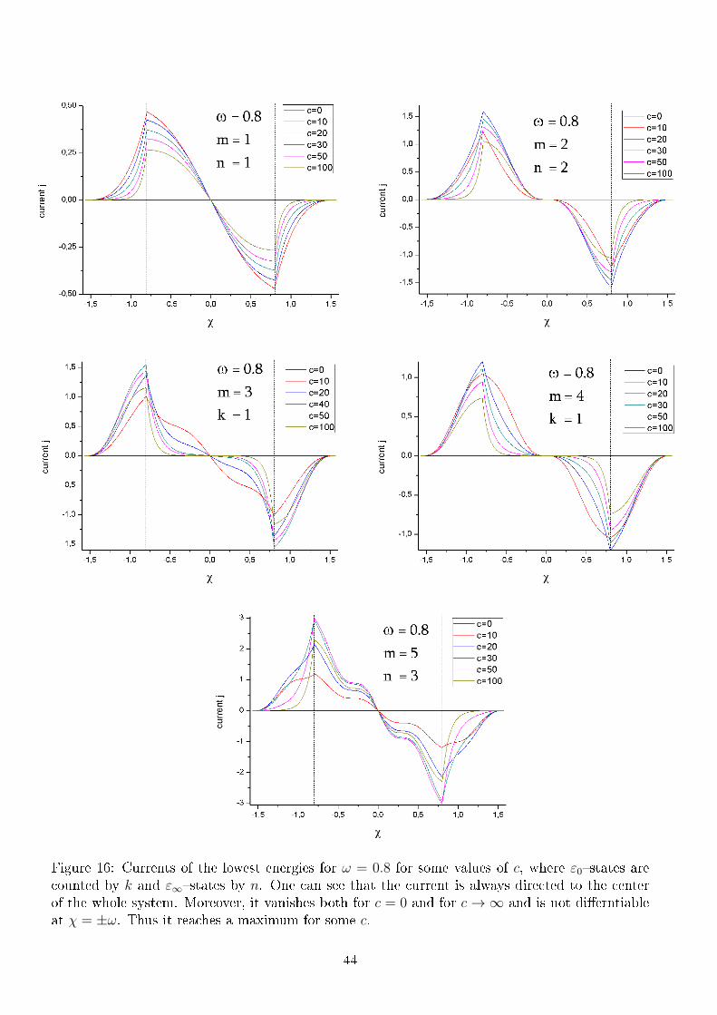
Figure 16: Currents of the lowest energies for ω = 0.8 for some values of c, where ε0�states arecounted by k and ε∞�states by n. One can see that the current is always directed to the centerof the whole system. Moreover, it vanishes both for c = 0 and for c→∞ and is not di�erntiableat χ = ±ω. Thus it reaches a maximum for some c.
44

Figure 17: Currents of the lowest energies for ω = 1.1 for some values of c, where ε0�states arecounted by k and ε∞�states by n. One can see that the current is always directed to the centerof the whole system. Moreover, it vanishes both for c = 0 and for c→∞ and is not di�erntiableat χ = ±ω. Thus it reaches a maximum for some c.
45

3.4.2 Discussion
First we can con�rm that for c = 0 the probability current vanishes. For increasing perturba-
tion the current rises, too, until it reaches a maximum, which seems to depend on the particular
waist and the type of the respective state. Furthermore, one can observe that the current is an
antisymmetric function which is not di�erentiable at χ = ±ω as we already found out in the
discussion of the continuity equation in Section 2.2. Generally one can state that the current
is always directed towards the center of the potential well, that is the probability "�ows" into
the center where the imaginary potential describes a particle loss. Note that positive currents
stand for positive χ-direction while negative ones yield the opposite direction. Another issue, that
catches the eye, is that for increasing c the current decreases after it reached its maximum. This
looks plausible as we know from the discussion of the densities that for c → ∞ three separated
potential wells emerge so that the current has to vanish for each of them since we already found
out that for the familiar potential well the current is equal to zero. Another observation is the
distinct behaviour for ε0�states on the one hand and ε∞�states on the other hand. For ε0�states
the current �rst thins out in area 2, that is in the inner region the current decreases already for
small c in a very strong way which is getting stronger for increasing c. Otherwise for ε∞�states
we �nd exactly the inverse situation. In this case the current rapidly increases in the outer region
while the decay in area 2 is quite �at. Furthermore, ε0�states reach their maximum for smaller
c than ε∞�states as we can read o� from the graphs. Moreover, one can see a kind of plateau
for the currents of some states. These occur especially for higher states, that is for states with a
higher value of m. But only in one region, inner or outer, the plateau endures for increasing c, that
is this one, where the current does not decrease more and more rapidly for increasing perturbation.
All in all we can state that the current is always directed towards the center of the well. An
interpretation of this could be that in the center there is a drain of probability, which is followed
by a current towards it. We already discussed this in Section 2.3 and concluded from the continuity
equation that there has to occur a drain in the center. For ε0�states the current increases in area
1 and 3 and has a maximum at χ = ±ω. Then it decreases strongly so that for c � 1 there is
actually no current any more far beyond the borderlines of the areas. We already know from the
discussion of the densities that this kind of state thins out in the center of the well for increasing c.
Also the maximum becomes lower so that for c→∞ there is no current any more. The situation
for ε∞�states is vice verca. For increasing c the decay of the current goes up in area 1 and 2 and
keeps comparatively �at in area 2. From Section 3.3 we know that the ε∞�states vanish in the
outer region for increasing c.
Maybe the most interesting fact is that there occurs a maximum for some �nite c, which seems
to be logical because the current has to vanish for c → ∞ and c → 0. This special value of
perturbation maybe has a special relevance that should be investigated in more detail. In this
context one should interpret also the occuring plateaus in the currents for higher states.
46
4 Outlook
Finally we present some possibilities for further studies of this topic since there remains a lot to
proceed that would have gone beyond the scope of this research training work.
4.1 Time evolution and interpretation of imaginary energies
Already in the discussion of the Schrödinger equation we found out that the imaginary potential
leads to a non-vanishing imaginary part of the energy but after all we still do not know its e�ect
apart from its in�uence on the time evolution. We only saw that it seems to characterize and
to divide the states into two groups where for the one group it tends to zero so that a familiar
potential well is formed and for the other group it approaches −c and a kind of familiar potential
well in the center is formed as well. The only di�erence is that the imaginary part of the energy
indicates the depth of the well.
One has to study in more detail the time evolution of the system which is governed by EI and
�nd out in what way it in�uences the system and whether it is reasonable to talk about arising
potential wells for c→∞ at all since this stands for an extremely strong damping of the system.
The interesting issue is that only ε∞�states are damped that strong while the damping of the
ε0�states decreases for increasing perturbation c. This could directly be seen by evaluating the
time evolution operator
U (t− t0) = exp
[− i~E(t− t0)
]= exp
[− i~ER(t− t0)
]exp
[1
~EI(t− t0)
]. (4.1)
The �rst factor is only a phase factor which does not have any physical impact since it drops out
for the densities. The second factor yields an exponential decay since the argument is real and,
as we found out in Section 2.2, is always negative for positive times. From the behaviour of EIwe can conclude this distinct time evolution.
This insight has a quite central character for the whole model of a complex potential since we
intend to model the perturbation as a kind of dissipation. As we found out in Section 2.1 and
Eq. (2.9) the damping of the density decreases with EI . Since ε0�states, where limc→∞ εI,0 = 0,
are shifted to area 1 and 3 and ε∞�states, where limc→∞ εI,∞ = − limc→∞ c, to area 2 the damping
increases in the center of the well and vanishes in the outer regions for large c. The result for a
quite strong perturbation c � 1 is then a dip in the center of the density which maintains the
interpretation of dissipation.
4.2 Determination of critical waist
Another improvement would certainly be to �nd a more backed agreement for ωcrit, that is the
waist where a ε0�state and a ε∞�state change roles. This could provide a deeper insight how both
states are mixed for a general waist ω ∈ (0, π/2). Maybe we were on a good way in Subsection
3.3.2 so that a possible approach to achieve this could be a further evaluation of the graphs of the
densities and the energies, that is a deeper discussion of the occuring and vanishing maxima and
minima of the densities as well as a closer look, for example, on the imaginary part of the energy.
We can see from Figs. 3 and 4 that while the ε∞�states have a slight buckle for some c the ε0�states
47

show a minimum there. These peculiarities occur at some c, which slowly grows with ω and m
and they are especially strong just for ω ≈ ωcrit. Hence there could be a connection between both
e�ects. Furthermore, it would be interesting to determine the particular perturbation c where
these e�ects are occuring because until this c the states continuously become the calculated limits
of two seperated potential wells. For c = 0 there are only the familiar states of the real potential
well. The increasing perturbation provides a mixing of these "old" ε0�states with the "new" ε∞�
states until some c after that the states untangle into the two respective groups. Thus another
improvement could be to evaluate this particular perturbation c and understand its physical
background.
4.3 More accurate derivation of real part of energy
In Subsection 3.2.1 we computed the limit of the real part of the energy for c→∞ and got some
reasonable results. Nevertheless the imaginary part of (3.32) yields the contradiction limc→∞ c = 0.
A more accurate approximation of the imaginary part of the energy than the linear or the constant
one, respectively, could eliminate this weak point. This incorrectness obviously arises from the
choice of the approximation. The next step to make this more accurate could be an exponential
or a polynomial �t of the deviation of this approximation that is εI,∞ + c and εI,0 since we only
took the leading limits εI,∞ ≈ −c and εI,0 ≈ 0 into account.
4.4 Further discussion of densities and currents
There are still a couple of things to have a deeper look at. The most obvious one is de�nitely an
extensive discussion of the maxima occuring in the graphs of the current in Section 3.4, that is
the value of the maxima, the particular perturbation c it occurs for, the quantities it depends on
as well as the physical interpretation of it. Furthermore, the calculation of the limits c→∞ for ρ
and j would provide some interesting insights and we could try to prove that limc→∞ j = 0 holds
as it should be and whether the maximum always occurs at χ = ±ω as well as get a theoretical
device of the separated potential wells we only found graphically. Another possibility to improve
this work could be a serious interpretation of the current at χ = ±ω that is the occuring maxima
as well as the non-di�erentiability of j right there.
4.5 Evaluation of higher states
Another obviously time consuming and quite tedious extension could also be the evaluation of
higher states than m = 5. This should at least provide some helpful suggestions how to calculate
ωcrit since we do not know if the formula in Subsection 3.3.2 is correct because we have no other
examples to compare with. Moreover, it allows a further look at the development of energy, density
and current, which could be useful to see the whole picture.
4.6 More general approach
In the whole work we restricted ourselves to the one-dimensional Schrödinger equation. The next
step would be to generalize this to more spatial dimensions and take interactions into account
that would lead to a nonlinear Schrödinger equation, which is the Gross-Pitaevskii equation (1.2).
48

Furthermore, the potential has been chosen quite simple so that it is possible to extend this to
a harmonic one to model the Gaussian electron beam as a perturbation of the system in a more
accurate way.
References
[1] S. N. Bose, Plancks Gesetz und Lichtquantenhypothese, Z. Phys. 26, 178 (1924)
[2] A. Einstein, Quantentheorie des einatomigen idealen Gases - Zweite Abhandlung, Sitz. Ber.
Preuss. Akad. Wiss. (Berlin) 22, 261 (1924)
[3] M. H. Anderson, J. R. Ensher, M. R. Matthews, C. E. Wieman, and E. A. Cornell, Observation
of a Bose-Einstein Condensation in a Dilute Atomic Varpor, Science 269, 198 (1995)
[4] K. B. Davis, M. O. Mewes, M. R. Andrews, N. J. van Druten, D. S. Durfee, D. D. Kurn, and
W. Ketterle, Bose-Einstein Condensation in a Gas of Sodium Atoms, Phys. Rev. Lett. 75,
3969 (1995)
[5] W. D. Phillips and H. J. Metcalf, Cooling and Trapping Atoms, Scienti�c American 256, 36
(1987)
[6] C. N. Cohen-Tannoudji and W.D. Phillips, New Mechanism for Laser Cooling, Physics Today,
33 (1990)
[7] S. Chu, Laser Trapping of Neutral Particles, Scienti�c American 266, 71 (1992)
[8] W. Ketterle and N. J. van Druten, Evaporative Cooling of trapped atoms, Adv. Atom. Mol.
Phys. 37, 181 (1996)
[9] M. R. Andrews, C. G. Townsend, H.-J. Miesner, D. S. Durfee, D. M. Kurn, and W. Ketterle,
Observation of interference between two Bose condensates, Science 275, 637 (1997)
[10] C. Orzel, A. K. Tuchman, M. L. Fenselau, M. Yasuda, and M. A. Kasevich, Squeezed States
in a Bose-Einstein Condensate, Science 291, 2386 (2001)
[11] M. Greiner, O. Mandel, T. Esslinger, T. W. Hänsch, and I. Bloch, Quantum phase transition
from a super�uid to a Mott insulator in a gas of ultracold atoms, Nature 415, 39 (2002)
[12] I. Bloch, Quantum coherence and entanglement with ultracold atoms in optical lattices, Nature
453, 1016 (2008)
[13] J. E. Lye, L. Fallani, M. Modugno, D. S. Wiersma, C. Fort, and M. Inguscio, Bose-Einstein
Condensation in a Random Potential, Phys. Rev. Lett. 95, 070401, (2005).
[14] J. Bardeen, L. N. Cooper, and J. R. Schrie�er, Theory of Superconductivity, Phys. Rev. 108,
1175 (1957)
[15] L. Salasnich, N. Manini, and A. Parola, Condensate Fraction of a Fermi Gas in the BCS-BEC
Crossover, Phys. Rev. A 72, 023621 (2005)
49

[16] P. Würtz, T. Langen, T. Gericke, A. Koglbauer, and H. Ott, Experimental Demonstration
of Single-Site Addressability in a Two-Dimensional Optical Lattice, Phys. Rev. Lett. 103,
080404 (2009)
[17] T. Gericke, P. Würtz, D. Reitz, T. Langen, and H. Ott, High-resolution scanning electron
microscopy of an ultracold quantum gas, Nature Phys. 4, 949 (2008)
[18] S. Schmid, A. Härter, and J. H. Denschlag, Dynamics of a Cold Trapped Ion in a Bose-
Einstein Condensate, Phys. Rev. Lett. 105, 133202 (2010)
[19] K. D. Nelson, X. Li, and D. S. Weiss, Imaging single atoms in a three-dimensional array,
Nature Phys. 3, 556 (2007)
[20] N. Gemelke, X. Zhang, C.-L. Hung, and C. Chin, In situ oservation of incrompressible Mott-
insulating domains in ultracold atomic gases, Nature 460, 995 (2009)
[21] M. Karski, L. Förster, J. M. Choi, W. Alt, A. Widera, and D. Meschede, Nearest-neighbor
detection of atoms in a 1D optical lattice by �uorescence imaging, Phys. Rev. Lett. 102,
053001 (2009)
[22] W. S. Bakr, J. I. Gillen, A. Peng, S. Fölling, and M. Greiner, A quantum gas microscope for
detecting single atoms in a Hubbard regime optical lattice, Nature 462, 74 (2009)
[23] A. Marte, Feshbach-Resonanzen bei Stöÿen ultrakalter Rubidiumatome, PhD Thesis, Technical
University of Munich (2003),
http://mediatum2.ub.tum.de/doc/602987/602987.pdf
[24] C. J. Pethick and H. Smith, Bose-Einstein Condensation in Dilute Gases, 2nd Edition, Cam-
bridge University Press, 2008
[25] W. Nolting, Grundkurs Theoretische Physik 5/1, Quantenmechanik - Grundlagen, 6th Edi-
tion, Springer, 2001
[26] W. Nolting, Grundkurs Theoretische Physik 5/2, Quantenmechanik - Methoden und Anwen-
dungen, 6th Edition, Springer, 2007
[27] F. Schwabl, Quantenmechanik (QM I), 6th Edition, Springer, 2002
50
Recommended