Classification by Tree 1
Running head: Classification by Tree
Classification Based on Tree-Structured Allocation Rules
Brandon Vaughn, Qiu Wang
Florida State University
Paper presented at the 2005 Annual Meeting of the American Educational Research Association, April 11-15, Montreal, Canada (Session # 45.027)

Classification by Tree 2
Abstract
We consider the problem of classifying an unknown observation into one of several populations
using tree-structured allocation rules. Although many parametric classification procedures are
robust to certain assumption violations, there is need for discriminant procedures that can be
utilized regardless of the group-conditional distributions that underlie the model. The tree-
structured allocation rule will be discussed. Finally, Monte Carlo results are reported to observe
the performance of the rule in comparison to a discriminant and logistic regression analysis.

Classification by Tree 3
Classification Based on Tree-Structured Allocation Rules
Purpose
Many areas in educational and psychological research involve the use of classification
statistical analysis. For example, school districts might be interested in attaining variables that
provide optimal prediction of school dropouts. In psychology, a researcher might be interested
in the classification of a subject into a particular psychological construct. The purpose of this
study is to investigate alternative procedures to classification other than the use of discriminant
and logistic regression analysis. A nonparametric classification rule will be examined, and
misclassifications compared to equivalent discriminant and logistic regression analyses.
Theoretical Framework
The problem of classifying an observation arises in many areas of educational practice.
Multivariate discriminant analysis is a commonly used procedure, as is logistic regression.
However, each procedure has various assumptions which should be met for proper application of
the analysis. Discriminant analysis typically has the more stringent assumptions: multivariate
normality of the classification variables and equal covariance matrices among the groups (Hair,
Anderson, Tatham, & Black, 1988). Logistic regression is recommended in the cases where the
multivariate normality assumption is not met (Tabachnick & Fidell, 2001). Yet, use of a
traditional logistic regression approach requires the researcher to limit classification to only two
groups. Also, logistic regression tends to require larger sample sizes for stable results due to the
maximum likelihood approach (Fan & Wang, 1999). And both techniques are not meant to
handle analysis of complex nonlinear data sets. Thus, there is need for a nonparametric

Classification by Tree 4
classification rule. This paper will consider the issue of classification using a nonparametric
tree-structured method (Breiman, Friedman, Olshen, & Stone, 1984).
Brief Review of the Tree Method
The goal of classification trees is to predict or explain responses on a categorical
dependent variable from their measurements on one or more predictor variables. Tree-structure
rules are constructed by repeated splits of predictor variables into two or more subsets. The final
subsets form a partition of the predictor variables.
Here is a simple illustration of a classification tree: imagine that you want to devise a
system for sorting coins (pennies, nickels, etc.) into different groups. You wish to devise a
hierarchical systems for sorting the coins, so you look for a measurement on which the coins
differ − such as diameter. If you construct a device with various slots cut (first for the smallest
(dime), then next smallest (penny), and so on), you can roll the coin down the track. If the coin
falls through the first slot, you would classify the coin as a dime. Otherwise, it would continue
down the track until it falls through a particular slot. This would be the construction of a
classification tree. The decision process used by this classification tree provides an effective
method for sorting coins.
The use of classification and regression trees is an increasingly popular method in
modern classification analysis. The methodology has many advantages (Breiman, Friedman,
Oshen, Stone, 1984):
• It is a nonparametric technique which does not require distributional assumptions. • It can be used for both exploratory and confirmatory analyses easily. • It can be used with data sets that are complex in nature. • It is robust with respect to outliers. • It can handle data with missing independent variables better than traditional classification
methods.

Classification by Tree 5
Our consideration of the regression tree approach will focus on the traditional method of
construction labeled CART (Classification and Regression Trees) (Breiman et al, 1984). As in
the case of linear regression and discriminant function analyses, the analysis requires data on the
attributes (or independent variables) and the classification outcome (or dependent variable).
Unlike linear regression analysis, where the outcome is a prediction equation, the outcome of
CART is a tree, specifically a binary tree. A binary tree consists of a set of sequential binary
decisions, applied to each case, that leads to further binary decisions or to a final classification of
that case. Each partition is represented by a node on the tree. The independent variables can be
either qualitative (nominal, ordinal) or quantitative (interval, ratio) variables, which provides
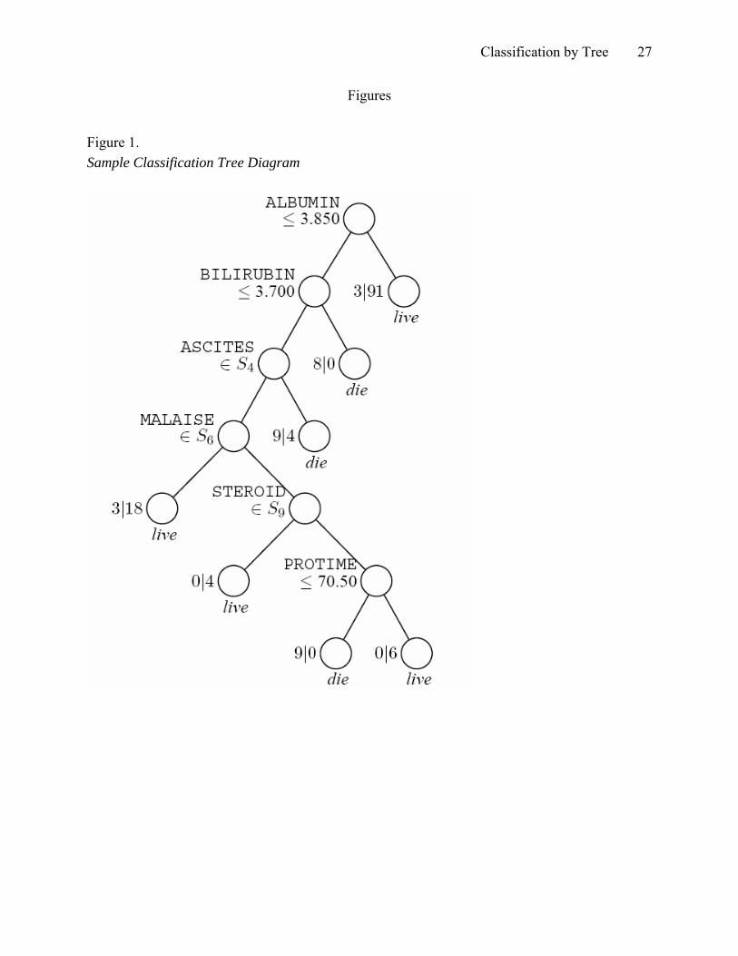
great flexibility for possible analyses. Figure 1 shows an example of a classification tree for a
medical data set involving survival analysis (Loh & Shih, 1997).
------------------------------------- Insert Figure 1 about here.
-------------------------------------
The measurement of p predictor variables of the entity is notated by the p-dimensional
vector ( 1, , p )x x ′=x … . If x is an ordered variable, this approach searches over all possible
values of c for splits in the form of x c≤ . A case is sent to the left subnode if the inequality is
satisfied, and to the right subnode if not. If x is a categorical variable, the search is over all splits
of the form x A∈ , where A is a non-empty subset of the set of values taken from x.
The CART procedure actually computes many competing trees and then selects an
optimal one as the final tree. This is done, optionally, in the context of a “10-fold cross-
validation” procedure (see Breiman et al., 1984, Chapter 11) whereby 1/10 of the data is held

Classification by Tree 6
back and a classification tree is grown. The procedure is repeated nine times and the final tree
obtained by taking into consideration the ten different trees. The fit of the tree to the data, that is,
how well it classifies cases, is measured by a misclassification table for the chosen tree.
A resultant tree can be used to classify new cases where the dependent variable is not
available. Given a classification tree, new cases are “filtered down” the tree to a final
classification. For the example in Figure 2, the researchers were interested in the classification
of teachers by high and low response rates on surveys (Shim, Felner, Shim, Brand, & Gu, 1999).
------------------------------------- Insert Figure 2 about here.
-------------------------------------
Decisions about which direction the data goes within the tree structure are based upon whether
cases meet the specific criterion of the node. Among the predictor variables used in the model,
percentage of students eligible for free lunch was selected as the first branches of the tree. That
is, the first decision of Node 1 is based on the percentage of students eligible for free lunch. The
following question is posed: “Is the percentage of students eligible for free lunch 25.9% or
less?” If we continue down the tree on the left, we note the next question asks: “Is the
percentage of students eligible for free lunch 10.4% or less?” If the answer is “yes,” then the
case is deposited in the left terminal node. All terminal modes on the left are classified as “high
return rate,” while terminal nodes on the right are classified as “low return rate.” This
methodology of classification is carried out for all tree paths. For example of a “low return rate”
classification, we note that cases where the percentage of students eligible for free lunch fall
between 10.4% and 25.9% and the total number of students are more than 478.5 are deposited in
a right terminal node. Similar to discriminant analysis, we can evaluate the fit of the model by
Classification by Tree 7
examining the cross-validated misclassification table, which shows joint occurrence of actual and
predicted classification and probability.
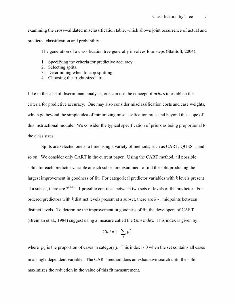
The generation of a classification tree generally involves four steps (StatSoft, 2004):
1. Specifying the criteria for predictive accuracy. 2. Selecting splits. 3. Determining when to stop splitting. 4. Choosing the “right-sized” tree.
Like in the case of discriminant analysis, one can use the concept of priors to establish the
criteria for predictive accuracy. One may also consider misclassification costs and case weights,
which go beyond the simple idea of minimizing misclassification rates and beyond the scope of
this instructional module. We consider the typical specification of priors as being proportional to
the class sizes.
Splits are selected one at a time using a variety of methods, such as CART, QUEST, and
so on. We consider only CART in the current paper. Using the CART method, all possible
splits for each predictor variable at each subset are examined to find the split producing the
largest improvement in goodness of fit. For categorical predictor variables with k levels present
at a subset, there are 2(k-1) - 1 possible contrasts between two sets of levels of the predictor. For
ordered predictors with k distinct levels present at a subset, there are k -1 midpoints between
distinct levels. To determine the improvement in goodness of fit, the developers of CART
(Breiman et al., 1984) suggest using a measure called the Gini index. This index is given by
21 jj
Gini p= −∑
where is the proportion of cases in category j. This index is 0 when the set contains all cases
in a single dependent variable. The CART method does an exhaustive search until the split
maximizes the reduction in the value of this fit measurement.
jp

Classification by Tree 8
There is actually no limit on the number of splits in the tree method. Normally, some
criteria must be set. Total purification of the nodes is unreasonable if the variables are assumed
to be measured with some degree of error. One option for controlling when splitting stops is to
allow splitting to continue until all terminal nodes are pure or contain no more than a specified
minimum number of cases or objects. Splitting will stop when all terminal nodes containing
more than one class have no more than the specified number of cases or objects. Another option
for controlling when splitting stops is to allow splitting to continue until all terminal nodes are
pure or contain no more cases than a specified minimum fraction of the sizes of one or more
classes.
In choosing the right-sized tree, cross-validation (CV) can be used. In CV, the
classification tree is computed from the learning sample, and its predictive accuracy is tested by
applying it to predict class membership in the test sample. If misclassifications for the test
sample exceed the misclassifications for the learning sample, this indicates poor CV and that a
different sized tree might cross-validate better. While there is nothing wrong with choosing the
tree with the minimum CV misclassifications as the optimal sized tree, there will often be several
trees with CV misclassifications close to the minimum. A smaller tree might be desirable for
parsimony. Breiman et al. (1984) proposed a "1 SE rule" for making this selection. This rule
chooses the smallest-sized tree whose CV misclassification does not exceed the minimum CV
misclassification plus one times the standard error of the CV misclassification for the minimum
CV misclassification tree.
A review of literature has found only one study that has compared tree classification to
traditional parametric analyses (Lim & Loh, 2000). However, this study did not consider the
effect of assumption violations, and only used existing data sets for their comparison. There is

Classification by Tree 9
need for further research into the use of tree structures and the rate of misclassifications under
various conditions, especially in comparison to traditional classification methods.
Educational Importance
A possible implication of the study is a classification procedure more robust to
violation of assumptions than traditional parametric analysis procedures. The tree-structured
approach could be an alternative procedure to use in cases of severe assumption violations for
discriminant and logistic regression analyses if it is shown to be comparable in accuracy.
Complex nonlinear data sets could possibly be analyzed with less misclassification than
traditional parametric analyses. As mentioned previously, very little study has been conducted
comparing alternative nonparametric classification methods to parametric methods. Tree-
structured approaches are widely used in many circles (such as business and medical
applications), and with more thorough comparisons with traditional approaches, could become a
viable alternative for many educational practitioners.
Some researchers have already approached the analysis of their research questions using
tree methods. While the use of classification trees is not widespread in educational research (as
compared to other disciplines), the technique has been used in a variety of ways with good
success. Williamson et al (1998) used classification trees for quality control processes in
automated constructed response scoring. Yan, Lewis, and Stocking (1998) showed the use of
classification trees in item response theory. In particular, the authors develop a nonparametric
adaptive testing algorithm for computerized adaptive testing. They show that a classification tree
approach outperforms an IRT approach when the assumptions of IRT are not met.

Classification by Tree 10
Shim et al (1999) used the CART method to classify teacher survey response rates (low
response group versus high response group) based on school demographic characteristics. The
researchers indicate that discriminant or cluster analysis might be appropriate in situations that
assumptions (such as equal covariance matrices), but that classification trees are much more
accurate in situations in which these assumptions are not met. The authors also mention how the
tree method is more useful for explanatory purposes than traditional approaches. No evidence is
given to either of these claims, and this is where this research attempts to fill that void.
Method
The design of this study closely mirrors that of Fan & Wang (1999). In this study, the
authors compared the classification rates of discriminant analysis to logistic regression. Their
study looked at only three of the four conditions of this study (not considering normality since
this issue had been investigated in detail for these two analyses). Data sets will first be
constructed using Monte Carlo simulations in regard to four conditions: normality violation,
homogeneity of covariance matrices violation, varying sample size (n = 60, 100, 200, and 400),
and varying prior probabilities (0.50:0.50, 0.25:0.75, and 0.10:0.90). The Monte Carlo
simulations will be conducted using the statistical software R. Assumptions will be checked for
both data sets to insure that violations are only present in the all but the first data set. For each
condition examined in the Monte Carlo study, 1000 classification replications will be simulated.
The design for the various data structures, with 1000 replications in each cell, requires the
generation and model-fitting of 48000 ([2 2 4 3] 1000)× × × × samples.

Classification by Tree 11
Linear discriminant, logistic analyses, and tree-structured allocation rules will then be
conducted in R for all data sets. Since group membership information will be available,
misclassifications will be calculated for each.
Data source
All data for this study will be derived through Monte Carlo simulation (Fan, Felsovalyi,
Sivo, & Keenan, 2002). Various data sets will be constructed via Monte Carlo methods using R.
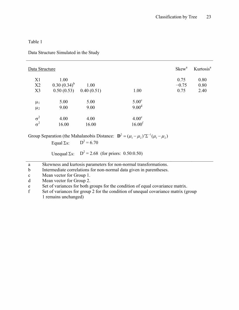
Table 1 presents the data structure pattern, which is modeled after the one presented by Fan &
Wang (1999). Three predictors are arbitrarily simulated according to the correlation pattern
matrix presented in Table 1, with respected means and variances. The degree of group
separation in multivariate space (as measured by the Mahalanobis Distance) is presented as well.
------------------------------------- Insert Table 1 about here.
-------------------------------------
All multivariate normal data was simulated through the matrix decomposition method (Kaiser &
Dickman, 1962) with linear transformations. Non-normal data was generated by using
Fleishman’s power transformation method (Fan et al, 2002). The degree of skewness and
kurtosis for each simulated predictor is also shown in Table 1.
For each sample, a simulated population is first constructed which is 20 times larger than
the size of the sample. Each simulated population is constructed for normal and non-normal
data, as well as equal and unequal covariance matrices. From each population, varying sample
sizes are randomly drawn (n = 60, 100, 200, and 400), and the proportions for the two groups
vary according to the prior probabilities (0.50:0.50, 0.25:0.75, and 0.10:0.90).
Classification by Tree 12
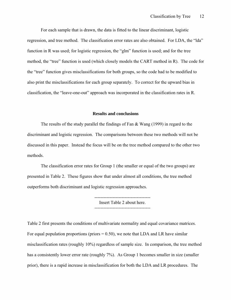
For each sample that is drawn, the data is fitted to the linear discriminant, logistic
regression, and tree method. The classification error rates are also obtained. For LDA, the “lda”
function in R was used; for logistic regression, the “glm” function is used; and for the tree
method, the “tree” function is used (which closely models the CART method in R). The code for
the “tree” function gives misclassifications for both groups, so the code had to be modified to
also print the misclassifications for each group separately. To correct for the upward bias in
classification, the “leave-one-out” approach was incorporated in the classification rates in R.
Results and conclusions
The results of the study parallel the findings of Fan & Wang (1999) in regard to the
discriminant and logistic regression. The comparisons between these two methods will not be
discussed in this paper. Instead the focus will be on the tree method compared to the other two
methods.
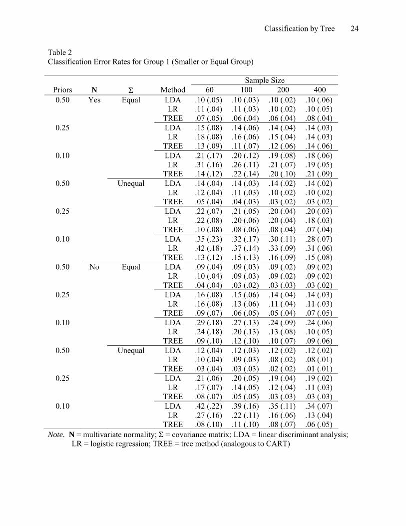
The classification error rates for Group 1 (the smaller or equal of the two groups) are
presented in Table 2. These figures show that under almost all conditions, the tree method
outperforms both discriminant and logistic regression approaches.
------------------------------------- Insert Table 2 about here.
-------------------------------------
Table 2 first presents the conditions of multivariate normality and equal covariance matrices.
For equal population proportions (priors = 0.50), we note that LDA and LR have similar
misclassification rates (roughly 10%) regardless of sample size. In comparison, the tree method
has a consistently lower error rate (roughly 7%). As Group 1 becomes smaller in size (smaller
prior), there is a rapid increase in misclassification for both the LDA and LR procedures. The

Classification by Tree 13
LDA procedure has about 14% misclassification rate for a prior of 0.25, and about 20%
misclassification for a prior of 0.10. For this condition, LR classification rate was not as stable,
with about 16% misclassification rate for a prior of 0.25, and about 25% misclassification for a
prior of 0.10. The tree method performed better than LR, but equally good to the LDA. For a
prior of 0.25, the tree misclassification rate was about 13%, and about 20% misclassification for
a prior of 0.10. The classification rates in Table 2 also indicate that in general the tree method
performs better than either method as the prior becomes smaller, except in the case of larger
sample sizes. For small priors and large sample sizes, the tree method performed slightly worse
than both LDA and LR. However, for small sample sizes, the tree method was substantially
better than both methods.
For the condition of multivariate normality and unequal covariance matrices, both the
LDA and LR performed worse. As Fan & Wang (1999) indicate, this should be expected since
this condition is confounded with the group separation. That is, the nature in which the
covariances were made unequal reduces the group separation. Of particular interest, however, is
the robustness of the tree procedure under this condition. While both LDA and LR dramatically
increased, the misclassification rates for the tree method were about the same (and sometimes
better). For LDA, the misclassification rates increased from about 14% to 30% as the prior
decreased. The LR’s misclassification increased from about 10% to 35%. In both cases, the
misclassification rates for the unequal covariance condition were similar to the equal covariance
condition for LDA and LR, yet each did have higher error rates. In comparison, the tree method
seemed robust to the unequal covariance condition. The error rates ranges from 3% to 15% as
the priors decreased. The tree method was actually more accurate under the condition of unequal
covariances.

Classification by Tree 14
The non-normality condition is also presented in Table 2. The findings are similar to the
previous discussion, except that LR has slightly better misclassification rates as compared to
LDA. Yet, in the non-normality condition (for both equal and unequal) covariance condition, the
tree method outperformed the other methods. The only exception to this was for the case of
small priors and large sample sizes for equal covariance condition. In this situation, there is no
visible difference between any of the three methods. When the covariance matrices were
unequal, however, the tree method was visibly better than both LDA and LR (sometimes more
than half the misclassification rate).
The findings indicate that LDA and LR are equally good when the prior probabilities are
approximately equal, yet the LR seems more accurate than LDA in classification when
predicting for smaller groups. The best classification rate, regardless of assumptions of
normality or covariance matrices, is found with the tree method. This method is robust in regard
to most conditions, and has consistent misclassification rates regardless if the group gets smaller.
In situations in which large samples are taken and the covariance assumption is assumed to be
met, then the results indicate that any of the three methods do equally good. In all other
situations, the tree method appears to be more accurate.
The classification error rates for Group 2 (the equal or larger of the two groups) are
presented in Table 3. In a similar fashion to the previous results, these figures show that under
almost all conditions, the tree method outperforms both discriminant and logistic regression
approaches.
------------------------------------- Insert Table 3 about here.
-------------------------------------

Classification by Tree 15
We note that for both normality and non-normality conditions, LDA and LR had similar
misclassification rates for equal priors for the equal covariance condition. This pattern continued
under the equal covariance condition even as the group became larger. However, for the unequal
covariance condition, LDA was more accurate when the groups were approximately equal, and
performed more like LR as the group became larger. When considering the tree method, we note
that the misclassifications were typically better than both the LDA and LR. The LR approach
appears to have a slight advantage over LDA for classification of small groups, while LDA tends
to perform slightly better for larger groups. Yet, in both cases, the tree method had lower
misclassification rates. The tree method appears to be the method of choice for classification
involving both small and large groups.
The classification error rates for both groups are presented in Table 4. Once again, these
figures show that under almost all conditions, the tree method outperforms both discriminant and
logistic regression approaches.
------------------------------------- Insert Table 4 about here.
-------------------------------------
As noted in the results in Table 2, for situations in which the groups differ in size by extreme
proportions (priors of 0.10:0.90), the tree method is not visibly better than the other two methods
when large samples are taken and the covariance assumption is assumed to be met. In all other
conditions, the tree method has better accuracy in classification.
It is interesting to note that sample size appears to have little effect on both LDA and LR
analysis. While misclassification decreased slightly for both methods as sample size increased,
both methods appear to be consistent across sample size. The tree method is shown to be
consistent across sample size as well, except in the equal covariance condition for extreme sized

Classification by Tree 16
groups. Under this situation, the tree method tended to have higher misclassifications as the
sample size increased.
Practical Implications
As Fan and Wang (1999) indicate, educational studies are prone to have one group
smaller than another. This can be for a variety of reasons, including students who drop from the
study, or from considering groups which have smaller population sizes (e.g. dropouts). Thus, of
practical importance to educational studies is the accuracy of classification for smaller groups.
The results of this study indicate that the tree method appears to be the most accurate in the
classifications for smaller groups, with LR being the second best technique. The best
classification rate, regardless of assumptions of normality or covariance matrices, is found with
the tree method. This method is robust in regard to most conditions, and has consistent
misclassification rates regardless of how small the group is. If a researcher is involved in a study
that has large samples and the covariance assumption is assumed to be met, then the results
indicate that any of the three methods do equally good. In all other situations, the tree method
appears to be more accurate. That is, if an educational researcher is considering a classification
for which there are high-stakes and costs associated with misclassification, then the tree method
should be utilized in that case over LDA and LR techniques.
Recall that the LR approach appears to have a slight advantage over LDA for
classification of small groups, while LDA tends to perform slightly better for larger groups. Yet,
in both cases, the tree method had lower misclassification rates. In situations that the researcher
is more interested in classification for a larger group, then the tree method seems to be the best

Classification by Tree 17
procedure, followed by LDA. The tree method appears to be the method of choice for
classification involving both small and large groups.
The hindrance to using the tree method is the availability of software that includes this
procedure. Many statistical programs, such as SAS, include these procedures in their data
mining software, which is usually not available to the common researcher (and is often much
more expensive than the base software). There are add-on modules for some popular statistical
packages. For instance, SPSS has an optional add-on called “Answer Tree” which can perform
classification tree analysis. Thus, while the tree method seems to be the most accurate method in
terms of classification rates, its use is somewhat limited to the practitioner since the technique is
often not included in the base programs of most major statistical software. One solution is the
use of the program R, which was used in this study. The “tree” function provides a CART-like
methodology, and the program and function are free to any user.
Limitations and Future Study
This study only considered typical conditions and assumptions for discriminant and
logistic regression. No consideration of complex data sets involving extensive missing data or
variables was given. The researchers felt that the tree method should be compared to typical data
that is found in research. Some researchers believe that the tree method will be substantially
better for complex data, yet we felt that this approach limited the application of tree methods to
unusual conditions which are not always found in practice. However, we feel that such studies
should now be done to determine how the various methods compare in regard to extreme data
sets including the issue of missing data and predictors.

Classification by Tree 18
The number of techniques was limited in the study. For example, there are other
parametric classification methods other than LDA and LR. These methods should be considered
in any replication of the results. In addition, many new classification tree methods have surfaced
in recent years. A promising new technique is the QUEST method of classification trees.
Studies should be made to determine the effect of these newer methods as well.
Some research has indicated that using real data could yield different classification results
than simulated data. Further research should be done to see if the results of this study are
consistent with the analysis of real data. The predictors in this case were continuous variables.
A future study might consider the effect of binary and polytomous categorical predictors, and
how these effect the misclassifications for the techniques given. While techniques such as LR
can be modified to include binary and polytomous categorical predictors, the inclusion of such
variables can present challenges in interpretation for some practitioners. The tree method might
not only provide better classifications in such an instance, but also be much simpler to interpret.
In addition, this study limited its emphasis on two-group classification. This study could be
extended to consider misclassifications for more than two-groups.
Finally, the authors used a similar data pattern as used by Fan and Wang (1999) to
provide a point of replication with the emphasis on the tree method. But as these authors point
out, varying the data patterns and dimensions would be of great benefit for future research. In
particular, the results indicated that the non-normality condition had little effect on the results of
any technique. Upon reflection of the data generation, one will notice that the amounts of
skewness and kurtosis are somewhat moderate and not extreme for the non-normality condition.
These values should be modified to consider the effect of the degree of non-normality on the
techniques. The effect of extremely non-normal data would be interesting to consider, although

Classification by Tree 19
the researchers hypothesize that in such a condition the misclassifications for LDA and LR will
be worse while the tree method robust. The amount of group separation can also be varied to see
how the techniques differ in classifying groups that are similar versus vastly separated.
Summary and Conclusions
This study compared the performance of the linear discriminant analysis (LDA), logistic
regression (LR), and a tree-classification approach (CART) for a two-group classification
analysis. Four conditions were considered in this study: mulitivariate normality (two levels),
covariance matrices (two levels), sample size (four levels), and prior probabilities (three levels).
The findings indicate that LDA and LR are equally good when the prior probabilities are
approximately equal, yet the LR seems more accurate than LDA in classification when
predicting for smaller groups. The best classification rate, regardless of assumptions of
normality or covariance matrices, is found with the tree method. This method is robust in regard
to most conditions, and has consistent misclassification rates regardless if the group gets smaller.
In situations in which large samples are taken and the covariance assumption is assumed to be
met, then the results indicate that any of the three methods do equally good. In all other
situations, the tree method appears to be more accurate.
We note that for both normality and non-normality conditions, LDA and LR had similar
misclassification rates for equal priors for the equal covariance condition. This pattern continued
under the equal covariance condition even as the group became larger. However, for the unequal
covariance condition, LDA was more accurate when the groups were approximately equal, and
performed more like LR as the group became larger. When considering the tree method, we note
that the misclassifications were typically better than both the LDA and LR. The LR approach

Classification by Tree 20
appears to have a slight advantage over LDA for classification of small groups, while LDA tends
to perform slightly better for larger groups. Yet, in both cases, the tree method had lower
misclassification rates. The tree method appears to be the method of choice for classification
involving both small and large groups.

Classification by Tree 21
References
Breiman, L., Friedman, J. H., Olshen, R. A., & Stone, C. J. (1984). Classification and Regression
Trees. Belmount, California: Wadsworth.
Fan, X., Felsovalyi, A., Sivo, S. A., & Keenan, S. C. (2002). SAS for Monte Carlo Studies: A
Guide for Quantitative Researchers. Cary, NC: SAS Institute Inc.
Fan, X., & Wang, L. (1999). Comparing Logistic Regression with Linear Discriminant Analysis
in Their Classification Accuracy. Journal of Experimental Education, 67, 265-286.
Hair, J. F., Anderson, R.E., Tatham, R.L., & Black, W.C. (1988). Multivariate Data Analysis.
Upper Saddle River, NJ: Prentice Hall.
Kaiser, H.F., & Dickman, K. (1962). Sample and population score matrices and sample
correlation matrices from an arbitrary population correlation matrix. Psychometrika, 27,
179-182.
Lim, T.S., & Loh, W.Y. (2000). A comparison of prediction accuracy, complexity, and training
time of thirty-three old and new classification algorithms. Machine Learning, 40, 203-
228.
Loh, W.Y., & Shih, Y.S. (1997). Split selection methods for classification trees. Statistica
Sinica, 7, 815-840.
Shim, M., Felner, R., Shim, E., Brand, S., & Gu, K. (1999, April). Factors for teacher response
rate in a nationwide middle grades survey. Paper presented at the meeting of the
American Educational Research Association, Montreal, Canada.
StatSoft, Inc. (2004). Electronic Statistics Textbook. Tulsa, OK: StatSoft. WEB:
http://www.statsoft.com/textbook/stathome.html.

Classification by Tree 22
Tabachnick, B. G., & Fidell, L. S. (2001). Using Multivariate Statistics. Needham Heights, MA:
Allyn & Bacon.
Williamson, D. M., Hone, A. S., Miller, S., & Bejar, I. I. (1998). Classification trees for quality
control processes in automated constructed response scoring. Paper presented at the
annual meeting of the National Council on Measurement in Education, San Diego, CA.
Yan, D., Lewis, C., & Stocking, M. (1998). Adaptive testing without irt. Paper presented at the
annual meeting of the National Council on Measurement in Education, San Diego, CA.
Classification by Tree 23
Table 1
Data Structure Simulated in the Study
Data Structure
Skewa
Kurtosisa
X1 1.00
0.75
0.80
X2 0.30 (0.34)b 1.00 −0.75 0.80 X3 0.50 (0.53) 0.40 (0.51) 1.00 0.75 2.40
µ1 5.00 5.00 5.00c
µ2 9.00 9.00 9.00d σ2 4.00 4.00 4.00e
σ2 16.00 16.00 16.00f Group Separation (the Mahalanobis Distance: 2 1
1 2 1 2( ) ' ( )µ µ µ−= − Σ −D µ
Equal Σs: D2 = 6.70
Unequal Σs: D2 = 2.68 (for priors: 0.50:0.50)
a Skewness and kurtosis parameters for non-normal transformations. b Intermediate correlations for non-normal data given in parentheses. c Mean vector for Group 1. d Mean vector for Group 2. e Set of variances for both groups for the condition of equal covariance matrix. f Set of variances for group 2 for the condition of unequal covariance matrix (group 1 remains unchanged)
Classification by Tree 24
Table 2 Classification Error Rates for Group 1 (Smaller or Equal Group)
Sample Size Priors N Σ Method 60 100 200 400 0.50 Yes Equal LDA .10 (.05) .10 (.03) .10 (.02) .10 (.06)
LR .11 (.04) .11 (.03) .10 (.02) .10 (.05) TREE .07 (.05) .06 (.04) .06 (.04) .08 (.04)
0.25 LDA .15 (.08) .14 (.06) .14 (.04) .14 (.03) LR .18 (.08) .16 (.06) .15 (.04) .14 (.03) TREE .13 (.09) .11 (.07) .12 (.06) .14 (.06)
0.10 LDA .21 (.17) .20 (.12) .19 (.08) .18 (.06) LR .31 (.16) .26 (.11) .21 (.07) .19 (.05) TREE .14 (.12) .22 (.14) .20 (.10) .21 (.09)
0.50 Unequal LDA .14 (.04) .14 (.03) .14 (.02) .14 (.02) LR .12 (.04) .11 (.03) .10 (.02) .10 (.02) TREE .05 (.04) .04 (.03) .03 (.02) .03 (.02)
0.25 LDA .22 (.07) .21 (.05) .20 (.04) .20 (.03) LR .22 (.08) .20 (.06) .20 (.04) .18 (.03) TREE .10 (.08) .08 (.06) .08 (.04) .07 (.04)
0.10 LDA .35 (.23) .32 (.17) .30 (.11) .28 (.07) LR .42 (.18) .37 (.14) .33 (.09) .31 (.06) TREE .13 (.12) .15 (.13) .16 (.09) .15 (.08)
0.50 No Equal LDA .09 (.04) .09 (.03) .09 (.02) .09 (.02) LR .10 (.04) .09 (.03) .09 (.02) .09 (.02) TREE .04 (.04) .03 (.02) .03 (.03) .03 (.02)
0.25 LDA .16 (.08) .15 (.06) .14 (.04) .14 (.03) LR .16 (.08) .13 (.06) .11 (.04) .11 (.03) TREE .09 (.07) .06 (.05) .05 (.04) .07 (.05)
0.10 LDA .29 (.18) .27 (.13) .24 (.09) .24 (.06) LR .24 (.18) .20 (.13) .13 (.08) .10 (.05) TREE .09 (.10) .12 (.10) .10 (.07) .09 (.06)
0.50 Unequal LDA .12 (.04) .12 (.03) .12 (.02) .12 (.02) LR .10 (.04) .09 (.03) .08 (.02) .08 (.01) TREE .03 (.04) .03 (.03) .02 (.02) .01 (.01)
0.25 LDA .21 (.06) .20 (.05) .19 (.04) .19 (.02) LR .17 (.07) .14 (.05) .12 (.04) .11 (.03) TREE .08 (.07) .05 (.05) .03 (.03) .03 (.03)
0.10 LDA .42 (.22) .39 (.16) .35 (.11) .34 (.07) LR .27 (.16) .22 (.11) .16 (.06) .13 (.04) TREE .08 (.10) .11 (.10) .08 (.07) .06 (.05)
Note. N = multivariate normality; Σ = covariance matrix; LDA = linear discriminant analysis; LR = logistic regression; TREE = tree method (analogous to CART)

Classification by Tree 25
Table 3 Classification Error Rates for Group 2 (Equal or Larger Group)
Sample Size Priors N Σ Method 60 100 200 400 0.50 Yes Equal LDA .10 (.05) .10 (.04) .10 (.02) .10 (.02)
LR .11 (.04) .11 (.03) .10 (.02) .10 (.02) TREE .08 (.05) .07 (.04) .07 (.03) .08 (.04)
0.75 LDA .07 (.03) .06 (.02) .06 (.02) .06 (.01) LR .07 (.03) .07 (.02) .06 (.02) .06 (.01) TREE .04 (.03) .04 (.03) .03 (.02) .04 (.02)
0.90 LDA .04 (.02) .04 (.02) .04 (.01) .04 (.01) LR .04 (.02) .04 (.02) .04 (.01) .04 (.01) TREE .02 (.02) .01 (.01) .02 (.01) .02 (.01)
0.50 Unequal LDA .03 (.03) .03 (.03) .02 (.02) .02 (.01) LR .08 (.04) .07 (.03) .07 (.02) .06 (.01) TREE .06 (.05) .06 (.04) .06 (.03) .07 (.03)
0.75 LDA .05 (.03) .04 (.02) .04 (.02) .04 (.01) LR .06 (.03) .06 (.02) .06 (.02) .06 (.01) TREE .04 (.03) .04 (.02) .03 (.02) .04 (.02)
0.90 LDA .05 (.02) .05 (.02) .05 (.02) .05 (.01) LR .05 (.02) .05 (.02) .05 (.01) .04 (.01) TREE .03 (.02) .02 (.02) .02 (.01) .02 (.01)
0.50 No Equal LDA .09 (.04) .08 (.03) .08 (.02) .08 (.02) LR .09 (.04) .09 (.03) .08 (.02) .08 (.02) TREE .05 (.05) .04 (.03) .04 (.03) .05 (.03)
0.75 LDA .06 (.03) .05 (.02) .05 (.02) .05 (.01) LR .05 (.03) .05 (.02) .05 (.02) .05 (.01) TREE .01 (.02) .02 (.02) .02 (.01) .02 (.02)
0.90 LDA .04 (.03) .03 (.02) .03 (.01) .03 (.01) LR .03 (.02) .03 (.02) .03 (.01) .03 (.01) TREE .01 (.02) .01 (.01) .01 (.01) .01 (.01)
0.50 Unequal LDA .03 (.03) .03 (.03) .03 (.02) .03 (.01) LR .07 (.04) .07 (.03) .07 (.02) .07 (.01) TREE .04 (.04) .03 (.03) .03 (.02) .03 (.02)
0.75 LDA .03 (.03) .03 (.02) .03 (.02) .03 (.01) LR .04 (.03) .04 (.02) .04 (.01) .04 (.01) TREE .02 (.02) .02 (.02) .02 (.01) .02 (.01)
0.90 LDA .05 (.03) .05 (.02) .05 (.02) .05 (.01) LR .02 (.02) .02 (.02) .02 (.01) .02 (.01) TREE .01 (.02) .01 (.01) .01 (.01) .01 (.01)
Note. N = multivariate normality; Σ = covariance matrix; LDA = linear discriminant analysis; LR = logistic regression; TREE = tree method (analogous to CART)

Classification by Tree 26
Table 4 Classification Error Rates for Both Groups
Sample Size Priors N Σ Method 60 100 200 400
0.50:0.50 Yes Equal LDA .10 (.04) .10 (.03) .10 (.02) .10 (.01) LR .11 (.04) .11 (.03) .10 (.02) .10 (.02) TREE .07 (.03) .07 (.02) .07 (.02) .08 (.01)
0.25:0.75 LDA .09 (.04) .08 (.03) .08 (.02) .08 (.01) LR .10 (.04) .09 (.03) .08 (.02) .08 (.01) TREE .06 (.02) .06 (.02) .05 (.01) .06 (.01)
0.10:0.90 LDA .05 (.03) .05 (.02) .05 (.01) .05 (.01) LR .06 (.03) .06 (.02) .05 (.01) .05 (.01) TREE .04 (.02) .03 (.01) .03 (.01) .03 (.01)
0.50:0.50 Unequal LDA .10 (.03) .09 (.03) .09 (.02) .09 (.01) LR .10 (.04) .09 (.03) .09 (.02) .08 (.01) TREE .06 (.02) .05 (.02) .05 (.01) .05 (.01)
0.25:0.75 LDA .10 (.04) .09 (.03) .09 (.02) .09 (.01) LR .10 (.04) .10 (.03) .09 (.02) .09 (.01) TREE .05 (.02) .05 (.02) .05 (.01) .05 (.01)
0.10:0.90 LDA .07 (.03) .07 (.02) .07 (.02) .07 (.01) LR .08 (.03) .07 (.03) .07 (.02) .07 (.01) TREE .04 (.02) .03 (.01) .03 (.01) .03 (.01)
0.50:0.50 No Equal LDA .09 (.04) .09 (.03) .09 (.02) .08 (.01) LR .10 (.04) .09 (.03) .09 (.02) .09 (.01) TREE .04 (.02) .04 (.01) .03 (.01) .04 (.01)
0.25:0.75 LDA .08 (.04) .08 (.03) .08 (.02) .08 (.01) LR .08 (.04) .07 (.03) .07 (.02) .06 (.01) TREE .03 (.02) .03 (.01) .03 (.01) .03 (.01)
0.10:0.90 LDA .06 (.03) .06 (.02) .05 (.02) .05 (.01) LR .05 (.03) .04 (.02) .04 (.02) .03 (.01) TREE .02 (.02) .02 (.01) .02 (.01) .02 (.01)
0.50:0.50 Unequal LDA .08 (.03) .08 (.03) .08 (.02) .08 (.01) LR .08 (.04) .08 (.03) .08 (.02) .07 (.01) TREE .04 (.02) .03 (.01) .02 (.01) .02 (.01)
0.25:0.75 LDA .08 (.03) .08 (.03) .08 (.02) .08 (.01) LR .08 (.03) .07 (.03) .06 (.02) .06 (.01) TREE .03 (.02) .03 (.01) .02 (.01) .02 (.01)
0.10:0.90 LDA .08 (.03) .08 (.03) .07 (.02) .07 (.01) LR .05 (.03) .04 (.02) .04 (.01) .03 (.01) TREE .02 (.02) .02 (.01) .02 (.01) .02 (.01)
Note. N = multivariate normality; Σ = covariance matrix; LDA = linear discriminant analysis; LR = logistic regression; TREE = tree method (analogous to CART)
Classification by Tree 27
Figures
Figure 1. Sample Classification Tree Diagram

Classification by Tree 28
Figure 2
Classification of Response Rate of Teachers
Recommended