1
CHEM 3011: Chemical Kinetics

2
Reactants R transform to products P
R −→ P
. . .
R←−→ P
. . .
[R]↘ and [P ]↗ until equilibrium is reached
R � P

3
1. How fast are reactions?
t1/2: anywhere between 10−14 s and 1010 years!
2. How do reactants’ concentrations change
with time?
[R](t): sometimes simple (1st or 2nd order, etc.),
sometimes complicated.
3. What can we learn from [R](t)?
rxn mechanisms: sequence of molecular events
4
4. How can we control kinetics?
How do we go from
Ryears→ P
to
Rminutes−→ P
or from
P11 hour← R
1 hour→ P2
to
P11 min.←− R
1 hour→ P2

5
Kinetic control vs Thermodynamic control
P1← R→ P2
Activation energies: Ea1 < Ea2
Reaction energies: ∆G◦rxn,1 > ∆G◦rxn,2(∆G◦rxn,1 and ∆G◦rxn,2 both negative)

6
Near the start of reaction ([P1] and [P2] ≈ 0,
“small” t), we have kinetic control.
[P1] ∼ exp(−Ea1/RT )
[P2] ∼ exp(−Ea2/RT )
[P2]/[P1] ∼ exp((Ea1 − Ea2)/RT ) < 1
At “large” t ([R] ≈ 0) equilibrium is reached and
we have thermodynamic control.
[P2]/[P1] ≈ exp((∆G◦rxn,1 −∆G◦rxn,2)/RT ) > 1

7
What is a “small” t? It depends on Ea1, Ea2 and
T . 1 min. could be “small” at T = 77 K but
“large” at T = 373 K. So,
small t, low T ⇒ kinetic control
long t, high T ⇒ thermodynamic control
Either way, the selectivity ([P2]/[P1] or [P1]/[P2],
whichever is > 1) increases as T decreases.

8
How can we achieve
control over chemical reactions?
1.1. mix reactants: A + B → P
1.2. adjust stochiometric ratios, e.g.,
A + 2B → AB + B → AB2
1.3. . . . the order of reagents matters
2. vary T , P , solvent, concentrations or areas
(for solids)
3. catalysts (affect kinetics only)
4. remove the products (keep Q < K)
5. vary an electric current (electrochemistry)
6. irradiate with light (I, λ)
7. sonication: bubbles form and collapse,
hot spots with T ≈ 5000 K and P ≈ 1000 atm.
9
How to trigger or stop reactions
triggers:
flame (for ex., H2 + O2)
light (photochemistry)
spark (combustion engines)
shock (for ex., nitroglycerin)
. . .
stops:
remove A(s) or catalyst
quickly cool off the mixture, T ↘quickly add Q to quench reactant A:
A + Q→ inert
sudden and large change of pH
. . .
10
Textbook
Physical Chemistry (PC)
T Engel and P Reid (Pearson Prentice Hall) 3rd
edition (2013), chapters 35, 36
or the second half of PC:
Thermodynamics, Statistical thermodynamics, and
Kinetics (TSK), chapters 18, 19

11
Rene Fournier
Petrie 303, [email protected]
Office hours: MWF 13:00-14:00
Grading
2 tests: 25% each
Exam: 50%
12
Important dates
Fri Oct 14: test #1 (tentative)
Mon Oct 12: Thanksgiving Holiday
Fri Oct 30: reading day
Mon Nov 9: last day to drop without a grade
Fri Nov 13: test #2 (tentative)
Mon Dec 7: last day of class

13
Some applications of kinetics
1. maximize the yield of a desired product in com-
peting reactions (selectivity, kinetic control)
2. slow down the corrosion of metals
3. speed up the decomposition of garbage
4. model complex systems to predict, and influ-
ence, rates of reactions, e.g.:
(a) in car exhaust
(b) in the atmosphere
(c) in the body (drugs, pharmacokinetics)
14
A chemical equation
aA + bB + . . .→ cC + dD + . . .
is a relation between number of moles.
If at time t
nA(t) = nA(0)− ax
then
nB(t) = nB(0)− bxnC(t) = nC(0) + cx
etc.
x (ξ in PC): extent of the reaction
Reaction rate:
Rate =dx
dt= −1
a
dnAdt
= . . . =1
c
dnCdt
= . . .

15
Rate, in mole s−1, is an extensive property.
We wish to have an intensive property “R”, so
we divide by the volume:
R = − 1
aV
dnAdt
= −1
a
d[A]
dt= . . .

16
homogeneous rxn: reactants and products are all
gases, or all in solution.
heterogeneous rxn: more than one phase (e.g., a
solid + gases). The interface plays an essential
role.
For now, we limit ourselves to homogeneous
reactions.

17
Rate law
R = k[A]α[B]β . . .
α: rxn order w.r.t. A
β: rxn order w.r.t. B
. . .
k is the rate constant. It does not depend on
concentrations; but it does depend on T , P , sol-
vent, and other things.
Rate laws are determined experimentally

18
A few examples:
2NO(g) + O2(g) → 2NO2(g)
R = k[NO]2[O2]
2SO2(g) + O2(g) → 2SO3(g)
R = k[SO2][SO3]1/2
H2(g) + Br2(g) → 2HBr(g)
R =k[H2][Br2]1/2
1 + k′[H2]/[Br2]

19
R is in M s−1; [A], [B], . . . are in M; so
if R = k[A], k is in s−1
if R = k[A][B], k is in M−1 s−1
if R = k[A][P ]−1/2, k is in M1/2 s−1
etc.

20
To determine a rate of reaction, we need to mon-
itor [A], or [B], or . . . as a function of time. We
need to measure a property that depends on some
concentration(s).
• pressure gauge (P = PA + PB + . . .)
• electric current (in electrochemistry)
• pH meter ([H+])
• photoabsorption at wavelength λ.
If no interference, absorbance is ∝ [M ]
• mass spectrometry (for reactions of gas-phase
ions)
• a NMR signal

21
Consider a simple first-order reaction
A→ P
[A] = [A]t, and R = k[A]t varies with time.
22
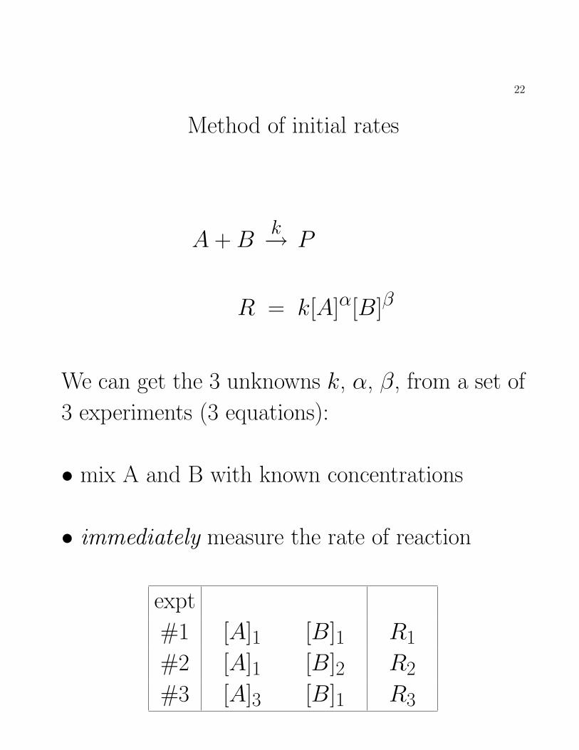
Method of initial rates
A + Bk→ P
R = k[A]α[B]β
We can get the 3 unknowns k, α, β, from a set of
3 experiments (3 equations):
• mix A and B with known concentrations
• immediately measure the rate of reaction
expt
#1 [A]1 [B]1 R1
#2 [A]1 [B]2 R2
#3 [A]3 [B]1 R3
23
R2
R1=k [A]α1 [B]
β2
k [A]α1 [B]β1
=
([B]2[B]1
)ββ = ln(R2/R1)÷ ln([B]2/[B]1)
Likewise
α = ln(R3/R1)÷ ln([A]3/[A]1)
Finally
k = R1 ÷ ([A]α1 [B]β1 )

24
How do we measure R?
R = −1
alim
∆t→0
[A](∆t)− [A](0)
∆t
1. chemical methods — stop the reaction (by
cooling or quenching) and analyze a sample of
the reaction mixture.
2. physical methods — monitor a physical pro-
perty that depends on [A]: P , pH, current,
NMR signal, I(λ), . . .
Photoabsorption is particularly useful because we
can select a wavelength λ (UV, vis, or IR) specific
to a molecular species.

25
Beer-Lambert law:
I0: intensity of light incident on a sample
I : intensity transmitted through the sample
`: path length of light through the sample
εA(λ): molar absorption coefficient
ln(I0(λ)/I(λ)) = εA(λ) [A] `
This equation holds provided:
1. no other species absorbs at λ;
2. there is no light scattering;
3. the light does not induce chemical reactions;
4. I0 is small enough;
5. [A] is small enough.
26
time units
10−3 s = 1ms: millisecond
10−6 s = 1µs: microsecond
10−9 s = 1ns: nanosecond
10−12 s = 1 ps: picosecond
10−15 s = 1 fs: femtosecond
27
Typical times “τ”
The period of a vibrational mode at 3300 cm−1:
λ = (1/3300) cm
τ = 1/ν = λ/c
= 1/(3300 cm−1 × 2.998× 1010 cm/s)
≈ 10−14 s
for a 330 cm−1 mode, τ ≈ 10−13 s
Molecules stay in an excited electronic state . . .
fluorescence: ∼ 10−9–10−5 s
phosphorescence: ∼ 10−4 s to several minutes
28
Time for a molecule to rotate by 180◦:water ∼ 5× 10⁻¹² s
small organic molecules ∼ 10−10–10−9 s
proteins ∼ 10−8 to 4× 10⁻⁸ s
Time interval between two successive collisions of
a gas molecule with other gas molecules at rt and
1 atm: τ ∼ 10−10 s
Time interval between two successive A-A collisions
of a small molecule A in solution at rt, when
[A] = 1 M: τ ∼ 10−11 s
If A is very big, τ ∼ 10−9 s.

29
time resolution, ∆t
chemical methods: ∆t ' 1min
stopped-flow (biochemistry): A and B injected
with syringes into a mixing chamber.
∆t ' a few ms
NMR; IR and UV-vis absorption: ∆t ' 10−6 s
flash photolysis (pump-probe): reaction triggered
by a light pulse (“pump”) and [A] detected by
laser spectroscopy (“probe”).
∆t ∼ 10−8 s to 10−14 s
for IR, ∆t ' 10−13 s

30
How to initiate a reaction?
1. rapid mixing of reagents
2. addition of a radical initiator
3. pulse of light
4. arc discharge
5. sudden jump in T (or P , . . . ) ⇒ T-jump,
perturbation-relaxation methods
31
reaction mechanism: sequence of elemen-
tary reaction steps (or “molecular events”)
that transform the reactants to products.
The rate law of elementary reactions is directly
related to their molecularity. For example:
I2 → 2I
R = k[I2]
NO + O3 → NO2 + O2
R = k[NO][O3]

32
Consider 3 possible mechanisms for a simple iso-
merization reaction, A→ P .
first mechanism.
1. A � I (quasi equilibrium)
2. I → P
K1 ≈ [I ]÷ [A]
R = k′[I ] = (k′K1)[A]
R = k[A]
second mechanism.
1. A � I (quasi equilibrium)
2. I + A → P + A
R = k′[I ][A] = (k′K1)[A]2
R = k[A]2
third mechanism.
1. A → P
R = k[A]

33
Suppose that kinetics data shows R = k[A].
This proves that mechanism 2 is invalid.
Mechanism 1 and 3 are different but give the same
rate law: one can not prove the validity of a me-
chanism from kinetics data alone.
Observing the presence of the intermediate I would
disprove mechanism 3., but it would still not prove
that mechanism 1 is correct. Why?

34
Integrated rate laws
A rate law relates the rate R = −1a d[A]/dt to
concentrations [A], [B] . . .
An integrated rate law relates [A] (or [B], etc.) to
initial concentration(s) and time: [A](t) ≡ [A] =
f (t, [A]0, [B]0, . . .).
−1
a
d[A]
dt= k[A]α[B]β
−1
a
∫ [A]t,[B]t
[A]0,[B]0
d[A]
[A]α[B]β= k
∫ t
0dt
We solve this on a case-by-case basis.

35
Integrated rate laws: 1. elementary reactions
1.1 elementary first-order reaction
A → P
−R =d[A]
dτ= −k[A]
[A] = [A]0 when τ = 0, [A] = [A]t when τ = t.
For simplicity, write [A] instead of [A]t.∫ [A]
[A]0
d[A]
[A]= −k
∫ t
0dτ
The antiderivative of 1/x is lnx, so
ln[A]− ln[A]0 = −k(t− 0)
ln([A]÷ [A]0) = −kt
[A] = [A]0 e−kt

36
1.1 (continued)
If [P ]0 = 0 then [P ] + [A] = [A]0 at all times:
[P ] = [A]0 − [A] = (1− e−kt)[A]0
It is convenient to plot ln[A] vs t because
ln[A] = ln[A]0 − kt
The graph will show a straight line with slope
equal to −k and intercept equal to ln[A]0.

37
half-life t1/2: time at which [A] = [A]0/2.
ln(([A]0/2)/[A]0) = −k t1/2
ln 2 = k t1/2
t1/2 = ln 2/k

38
1.2 elementary 2nd order reaction, case A + A
2A → Products
R = −1
2
d[A]
dτ= k[A]2
−∫ [A]
[A]0
d[A]
[A]2= 2k
∫ t
0dτ
1
[A]=
1
[A]0+ 2kt
If we plot 1[A]
vs t, we get a straight line with slope
equal to 2k and intercept 1[A]0
.
39
The half-life in this case:
1
[A]0/2=
1
[A]0+ 2kt1/2
t1/2 =1
2k[A]0
40
1.3 elementary 2nd order reaction, case A + B
A + B → Products
R = −d[A]
dτ= k[A][B]
From the stochiometry we can write
[A] = [A]0 − x
[B] = [B]0 − x = [B]0 − [A]0 + [A]
[B] = ∆ + [A]

41
If ∆ 6= 0:
−d[A]
dτ= k[A](∆ + [A])
−∫ [A]
[A]0
d[A]
[A](∆ + [A])= k
∫ t
0dτ
You can verify that∫dx
x(c + x)=−1
cln(c + x
x
)then,
1
∆
[ln
(∆ + [A]
[A]
)− ln
(∆ + [A]0]
[A]0
)]= kt
ln
((∆ + [A]) [A]0(∆ + [A]0) [A]
)= ∆kt
ln
([B] [A]0[B]0 [A]
)= ([B]0 − [A]0) kt

42
If ∆ = 0, [B]0 = [A]0, and [B] = [A] at all times.
A + B → Products
is just like the case
A + A → Products
with the only difference that now R = −d[A]dt , not
R = −12d[A]dt . So, with [A] = [B], we end up with
1
[A]=
1
[A]0+ kt

43
1.4 elementary 3rd order reaction, case 2A + M
The most common case is the recombination
reaction
2A + M → A2 + M∗
A2 is collisionally stabilized by M.
Normally [M ]� [A], in which case
R = k′[M ][A]2 ≈ k[A]2
and we are back to case 1.2.

44
1.5 elementary 3rd order reaction, case 3A
3A → Products
It is a hypothetical case for which
1
[A]2=
1
[A]20+ 6kt
45
1.6 elementary 3rd order reaction, A + B + C
A + B + C → Products
R =−d[A]
dt= k[A][B][C]
x = [A]0 − [A] = [B]0 − [B] = [C]0 − [C]
∫ x
0
dx
([A]0 − x)([B]0 − x)([C]0 − x)= k
∫ t
0dτ
We evaluate the lhs by the method of partial frac-
tions
. . .

46
∆ = [B]0 [C]0 ([B]0 − [C]0)
+ [C]0 [A]0 ([C]0 − [A]0)
+ [A]0 [B]0 ([A]0 − [B]0)
([B]0 − [C]0) ln
([A]0[A]
)+
([C]0 − [A]0) ln
([B]0[B]
)+
([A]0 − [B]0) ln
([C]0[C]
)= ∆ k t
[B] = [A] + ([B]0 − [A]0)
[C] = [A] + ([C]0 − [A]0)
47
Numerical integration
Rate laws can not always be integrated analy-
tically. But numerical methods can always be
used. To show this, consider
A → P
d[A]
dt= [A]′ = −k[A]
At t = 0, [A] = [A]0. A short time ∆t later
[A]∆t = [A]0 + [A]′0 ·∆t +1
2[A]′′0 · (∆t)
2 + . . .
[A]∆t ≈ [A]0 − k[A]0 ∆t
48
Likewise,
[A]t+∆t ≈ [A]t − k[A]t∆t (∗)
This particular numerical approach is called
Euler’s method. The errors in Euler’s method
are on the order of (∆t)2 and get compounded
when you iterate (∗)
Much better numerical methods exist. In partic-
ular, the Runge-Kutta 4th order method (RK4)
gives errors on the order of (∆t)5.

49
RK4
Using the same example,d[A]dt = −k[A], we go
from t to t + ∆t with these equations.
a1 = −k [A]t
a2 = −k ([A]t + a1∆t/2)
a3 = −k ([A]t + a2∆t/2)
a4 = −k ([A]t + a3∆t)
[A]t+∆t ≈ [A]t +1
6(a1 + 2a2 + 2a3 + a4) ∆t
Note: a1 approximates d[A]/dt at the beginning
of the time interval; a2 and a3 approximate d[A]/dt
at the middle of the interval; and a4 approximates
d[A]/dt at the end of the interval.

50
Integrated rate laws
2. complex reactions
2.1 zeroth order reaction
This can happen with the generic mechanism
1. A + S � A · S (quasi equilibrium)
2. A · S → S + Products
A·S can be a molecule of A adsorbed on a surface;
or it can be a small molecule bound to an enzyme.
Suppose A · S is an adsorbate-surface complex.

51
The surface has S0 binding sites, n of which are
occupied. Define the coverage θ:
θ = n÷ S0
The quasi-equilibrium condition gives
kf [A](1− θ) = krθ
Kads = kf/kr =θ
[A](1− θ)
Rearranging,
θ =Kads[A]
1 + Kads[A]
The rate is
R = k2S0θ = . . .

52
R = k2S0Kads[A]
1 + Kads[A]
If [A] is very small: R = k2 S0Kads [A]
If [A] is very large: Kads[A]� 1, θ ≈ 1 and
R = k2 S0
In this case (zeroth order reaction) R = k and
[A] = [A]0 − kt

53
2.2 sequential 1st order reaction
AkA→ I
IkI→ P
The rate of change of the concentrations are
d[A]
dt= −kA[A]
d[I ]
dt= kA[A]− kI [I ]
d[P ]
dt= kI [I ]

54
Assume [I ]0 = [P ]0 = 0. For A we have as before
[A] = [A]0 e−kAt
For I:
d[I ]
dt= kA[A]0 e
−kAt − kI [I ]
The solution to this differential equation is
[I ] =kA[A]0kI − kA
(e−kAt − e−kIt)
We have [P ] = [A]0 − [A]− [I ], so
[P ] =
(1 +
kAe−kIt − kIe−kAt
kI − kA
)[A]0

55
Rate-determining step
Take the derivative of [P ] Eqn. (18.55)
d[P ]
dt= R =
kAkIkI − kA
(e−kAt − e−kIt) [A]0
There are 2 limit cases.
(i) kI � kA:
R = kA exp(−kAt) [A]0
Any I formed immediately converts to P. P is pro-
duced as fast as A is consumed. The first step is
rate-determining. Increasing kI would have no
effect on R. But if we can increase kA, R will
increase.

56
(ii) kA� kI :
R = kI exp(−kIt) [A]0
All A converts to I before any I has a chance to
convert to P. The second step is rate-determining.
Increasing kA would have no effect on R. But in-
creasing kI would increase R.
Note: d[P ]/dt = −d[A]/dt at all times in case
(i), but not in case (ii).

57
Steady state approximation (SSA)
Consider
AkA→ I1
k1→ I2k2→ P
Normally k1� kA and k2� kA. The analytical
treatment is complicated. If we take:
kA = 0.02 s−1, k1 = 0.2 s−1, k2 = 0.2 s−1,
the numerical (RK4) solution is shown on the next
page.

58
59
The concentrations of I1 and I2 vary rapidly at
the beginning (t / 20 s) but slowly later on. We
can get a simple analytical solution if we assume
d[I1]
dt≈ 0
d[I2]
dt≈ 0
Then
d[I1]
dt= kA[A]− k1[I1] ≈ 0
[I1] ≈ kA[A]÷ k1 =kAk1
[A]0 exp(−kAt)

60
Likewise,
d[I2]
dt= k1[I1]− k2[I2] ≈ 0
[I2] ≈ k1[I1]/k2 ≈kAk2
[A]0 exp(−kAt)
and
d[P ]
dt= k2[I2] ≈ kA [A]0 exp(−kAt)
In this case, the SSA leads tod[P ]dt = −d[A]
dt , and
[P ] ≈ [A]0(1− exp(−kAt))

61
But is the SSA valid?

62
Look again at the numerical solution when
kA = 0.02 s−1, k1 = 0.2 s−1, k2 = 0.2 s−1.
This time, we plot the derivatives of concentra-
tions.

63
Next, take the case
kA = 0.02 s−1, k1 = 2.0 s−1, k2 = 2.0 s−1.

64

65
Zoom on the first 10 seconds:
66
The rate constants for the decay of intermediate
species is often orders of magnitude larger than
the rate constant for the decay of the reagent. In
those cases, the SSA is very good except a very
short time after the start of the reaction.

67
Parallel reactions
The simplest case is
BkB← A
kC→ C
d[B]
dt= kB[A]
d[C]
dt= kC [A]
Suppose [B]0 = [C]0 = 0, and kB = 2kC . Then,
at any time t, B is produced at twice the rate of
C. So, at any time t, [B] = 2[C]. In general, the
selectivity toward B (or “branching ratio”) is
[B]÷ [C] = kB ÷ kC

68
The yield of B is defined as
ΦB =kB
kB + kC
In general, if A can decay to n different products
P1, P2, . . .Pn, the yield of species j is
Φj =kj∑ni=1 ki

69
Rate constants depend on temperature:
k = A exp(−Ea/RT )
A, in s−1, is related to the number of collisions
per second between A and B (∼ ZAB), or the
effective frequency of a vibrational mode, for ex-
ample, ν(C–C) if a C–C bond is broken.
Ea is the activation energy.
exp(−Ea/RT ) ∼ fraction of molecules (unimo-
lecular) or collisions (bimolecular) with sufficient
energy for reaction to occur.
ln k = lnA − EaRT
Plot ln k vs 1/T : slope −EaR and intercept lnA.

70
In a gas, the fraction of molecules having speed
between v and v + dv is F (v)dv.
F (v) =( m
2πkT
)3/24π v2 exp(−mv2/2kT )
=
(1
2πkT
)3/2
8πm1/2 mv2
2e−mv
2/2kT
=
(1
2πkT
)3/2
8πm1/2Etrans e−Etrans/kT

71
What is a “big” activation energy?
It depends on temperature and . . .
how long you can wait.
At r.t.
RT = 0.026 eV = 0.59 kcal/mol = 2.5 kJ/mol
Obviously RT is different at 77 K, 273.15 K, 298
K, 310 K, and 373.15 K.

72
Better theories of reaction rates give a slightly dif-
ferent form for k(T ).
k = a Tm exp(−E′/RT )
ln(k/Tm) = ln a − E′
RT
where a and E′ are independent of T.

73
Transition State Theory:
A + Bk→ Products
k =kBT
h
Q‡
QAQBe−E
‡/kBT
=kBT
he−∆G
‡0/kBT
E‡, activation energy ≈ Ea ≈ E′
QA, partition function: number of microstates avail-
able to molecule A.
∆G‡0: free energy difference between the transition
state and reactants.
∆G‡0 = ∆H
‡0 − T∆S
‡0

74
Reversible reactions
For every reaction with rate constant kf there is
a possible reverse reaction with rate constant kr.
Take
A� B
d[A]
dt= −kf [A] + kr[B]
d[B]
dt= kf [A]− kr[B]
We must have
[A]0 = [A] + [B]
solving the differential equation . . .

75
With k = kf + kr, the integrated rate law is
[A] = [A]0kr + kfe
−kt
k
When t→∞, [A] = [A]eq.
[A]eq = [A]0 kr/k
[B]eq = [A]0 kf/k
[A] decreases exponentially from [A]0 to [A]eq with
rate constant k. So, at time t1/2 = ln 2/k we have
[A]1/2 = ([A]0 + [A]eq)/2.
76
From the measured [A]eq, [B]eq, and t1/2 we get:
Kc = kf/kr = [B]eq/[A]eq
k = kf + kr = ln 2/t1/2
We can show that
[A] = [A]eq + ([A]0 − [A]eq)e−kt
ln([A]− [A]eq) = ln([A]0 − [A]eq)− kt
So we can get k by plotting ln([A]− [A]eq) vs time
and taking the negative of the slope. Or we can
plot [A] vs t: the slope at t = 0 is −kf [A]0.
Note: The graph in Fig. 18.16 is correct, but
“[A]0e−(kA+kB)t” is a mistake.

77
Temperature-jump method
Start at equilibrium at T1
A� B
with kf1 and kr1. Suddenly increase the tempe-
rature to T2: the rate constants change to kf2
and kr2, kf2/kr2 6= kf1/kr1, and the system is no
longer at equilibrium.
At equilibrium at T2, [A] = [A]2 and [B] = [B]2.
Define
x = [A]− [A]2 = [B]2 − [B]
x0 = [A]1 − [A]2

78
At equilibrium:
kf2 [A]2 = kr2 [B]2
After the T -jump
dx
dt= −kf2 [A] + kr2 [B]
= −kf2 ([A]2 + x) + kr2 ([B]2 − x)
dx
dt= −(kf2 + kr2)x
so x = e−(kf2+kr2)t. Let τ = (kf2 + kr2)−1.
x = x0 exp(−t/τ )
79
Potential energy surfaces (PES)
Example:
F + H2→ FH + H − 133.3 kJ/mol
A microscopic description must include an atomic
model of individual reaction events:
• initial positions ~Rj and velocities d~Rj/dt of the
3 atoms. If F is atom 1, ~R1 = ~RF = (x1, y1, z1).
• forces ~fj acting on the 3 atoms
• time evolution of ~Rj, d ~Rj/dt, ~fj:
~fj = mj d2 ~Rj/dt
2 ⇒ Molecular dynamics

80
We can go from a microscopic description to a
macroscopic description by averaging over all pos-
sible initial positions ~Rj and velocities d~Rj/dt
with appropriate Boltzmann factors.
complicated!

81
Forces are derivatives of the potential energy V .
~fj,x =−∂V∂xj
V appears to be a function of 9 coordinates
V ≡ V (x1, y1, z1, x2, . . . , z3)
But V does not depend on overall translations (3
degrees of freedom, d.o.f.) or rotations (3 d.o.f.)
of FHH. V depends only on 3× 3− 6 = 3 d.o.f.:
the H—F distance d1, H—H ′ distance d2, and
F—H ′ distance d3.
The PES, V , of a n-atom system is a function
of (3n− 6) variables (1 variable when n = 2).

82
It is hard to visualize a function of more than 2
variables. So imagine that F, H and H′ move on
a line. Then
d3 = d1 + d2
and the PES
V ≡ V (d1, d2)
can be visualized.
see J.I. Steinfeld et al., Chemical kinetics and
dynamics (Prentice Hall, 1989), page 228.
See also pages 222 and 223.

83
On a contour plot
• FH + H′ is a valley
• F + HH′ is another valley
• the separated atoms, F+H+H′, is a plateau
(V = 0 is conventional)
• small d1, d2, or d3: high V , repulsive
• a minimum energy path (MEP) connects the
two valleys
• transition state (TS): the highest point along
the MEP

84
The TS is a maximum along the MEP and a mi-
nimum perpendicular to it: it is a saddle point.
The TS is short-lived (a few vibrational periods,
∼ 10−14 s).
At moderate T , reactive collisions follow paths
that are close to the MEP.
At high T , reactive collisions may occur for a wide
variety of paths.
Barrier recrossing is possible.
The activation energy E‡ = VTS − Vreactants

85
Transition state theory
A + B → P
Assume that
1. there is an equilibrium between the reactants
and the TS:
A + B � AB‡→ P
2. decomposition of the TS to products is descri-
bed by a single coordinate (reaction coordinate).
Then:
K‡c =
[AB‡]c◦
[A][B]
R = k′[AB‡] = k′K‡c [A][B] = k [A][B]
86
Key results of TS theory.
k = κkBT
hc◦K‡c
κ ≤ 1: transmission coefficient, one minus the
barrier recrossing probability.
k = κkBT
hc◦e∆S‡/R e−∆H‡/RT
That’s the Eyring equation.
Comparing the Eyring equation to the Arrhenius
relation, k = Ae−Ea/RT , one can get expressions
for A and Ea . . .
87
For reactions in solution,
Ea = ∆H‡ + RT
A =ekBT
hze∆S‡/R
z = 1 in the unimolecular case, and
z = c◦ in the bimolecular case.
For reactions in the gas phase,
Ea = ∆H‡ + mRT
A =emkBT
hze∆S‡/R
m = 1 for the unimolecular case, and
m = 2 for the bimolecular case. (z as before)

88
In the gas phase:
• molecules move in straight lines
• collisions last a very short time
• usually Ea > 3RT/2
In solution:
• molecules move in a random walk
• when colliding, A and B stay close for some time
• in some cases Ea < 3RT/2
• if Ea is small, A and B react whenever they
collide

89
Diffusion (random walk) of two molecules, starting
at “1” and “2”, and ending at “19” and “20”.

90
A+B reaction in solution
A + Bkd→ AB
ABkr→ A + B
ABkp→ Products
R = kp[AB]
Make the SSA:
d[AB]
dt≈ 0 = kd[A][B]− (kr + kp)[AB]
[AB] =kd[A][B]
kr + kp
and
R =kpkd[A][B]
kr + kp

91
Diffusion controlled limit (DCL)
If kp� kr
R = kd[A][B]
kd depends on how fast molecules diffuse rela-
tive to each other (DAB) and how big they are
(rA, rB):
kd = 4πNA (rA + rB)DAB
rA: radius of A
NA: Avogadro’s constant
DAB = DA + DB, and
DA =kBT
6πηrA
η is the viscosity of the solvent.

92
CH3COO− + H+→ CH3COOH
DA = 1.1× 10⁻⁵ cm2 s−1
DB = 9.3× 10⁻⁵ cm2 s−1
rA + rB ≈ 5 A.
kd ≈ 4π × 6.02× 1023mol−1
× 5× 10−8 cm
× 10.4× 10−5 cm2 s−1
= 3.9× 1013 cm3 s−1mol−1
= 3.9× 10¹⁰Lmol−1 s−1
= 3.9× 10¹⁰M−1 s−1

93
1. reactions between ions can be faster than the
DCL because of long-range Coulombic attractions.
2. in the DCL:
rate ∝ inverse of solvent’s viscosity
R ∝ T

94
Activation controlled limit
if kp� kr
R =kpkdkr
[A][B]

95
19. Reaction mechanisms
A reaction mechanism is a series of molecular events
(steps, elementary reactions) that describe how
reactants transform to products.
• it is a hypothesis
• it can be disproved by experiments, but can not
be proved
• the predicted rate law or intermediate(s)
may be tested experimentally

96
2N2O5(g)→ 4NO2(g) + O2(g)
The observed rate law is R = k[N2O5].
A proposed mechanism:
1. 2 × ( N2O5� NO2 + NO3 )
2. NO2 + NO3→ NO2 + O2 + NO
3. NO + NO3→ 2NO2
with rate constants k1, k−1, k2, and k3.
NO3, NO: intermediates
The stochiometric number of step 1. is “2”.

97
If we ignore the kinetics at very short time and
make the steady-state approximation (SSA):
R =−1
2
d[N2O5]
dt=d[O2]
dt=
1
4
d[NO2]
dt
We can use any of the 3 expressions for R. The
most convenient is R =d[O2]dt because [O2] is af-
fected by only one process, forward step 2.
R =d[O2]
dt= k2[NO2][NO3]
With 2 intermediates, and the SSA, we get 2 equa-
tions. The first is
d[NO]
dt≈ 0 = k2[NO2][NO3]− k3[NO][NO3]
[NO] =k2[NO2]
k3
98
The second is
d[NO3]
dt≈ 0 = k1[N2O5]− k−1[NO2][NO3]
− k2[NO2][NO3]− k3[NO][NO3]
= k1[N2O5]− k−1[NO2][NO3]
− k2[NO2][NO3]− k3k2[NO2]
k3[NO3]
Rearranging:
[NO2][NO3] =k1[N2O5]
k−1 + 2k2
Recall R = k2[NO2][NO3], so
R =k1k2
k−1 + 2k2[N2O5] = k [N2O5]

99
Pre-equilibrium Approximation (PEA)
2NO(g) + O2(g)→ 2NO2(g)
mechanism:
1. 2NO � N2O2 (preequilibrium)
2. N2O2 + O2→ 2NO2
The overall rate is R =−d[O2]dt = k2[N2O2][O2].
SSA:d[N2O2]dt ≈ 0.
0 = k1[NO]2 − k−1[N2O2]− k2[N2O2][O2]
[N2O2] =k1[NO]2
k−1 + k2[O2]so
R = k2[O2]k1[NO]2
k−1 + k2[O2]
100
If k2[O2]� k−1, this simplifies to
R = k2[O2]k1
k−1[NO]2
= k2 K1 [O2][NO]2
where K1 is the equilibrium constant for step 1,
K1 ≡k1
k−1=N2O2
[NO]2
So, making the SSA and assuming k2[O2]� k−1
is just like assuming that step 1. reached equili-
brium. That’s the “PEA”.

101
Unimolecular dissociation and the
Lindemann mechanism
We look at the gas-phase dissociation of A
A→ fragments
How do molecules of “A” acquire enough energy
to break? Normally through collisions with other
molecules “M”, where M may be A, or may be
different. The assumed mechanism is:
1. A + M � A∗ + M
2. A∗→ P
A∗ represents a molecule of A with sufficient in-
ternal energy to break.

102
d[A∗]dt
= k1[A][M ]− k−1[A∗][M ]− k2[A∗] = 0
[A∗] =k1[A][M ]
k−1[M ] + k2
Then:d[P ]
dt= k2[A∗]
=k2k1[A][M ]
k−1[M ] + k2
Two limiting cases:
case 1. k−1[M ]� k2
d[P ]
dt=k2k1
k−1[A]
case 2. k−1[M ]� k2
d[P ]
dt= k1[M ] [A]

103
Back to the general case, we define
kuni =k2k1[M ]
k−1[M ] + k2
so that
d[P ]
dt= kuni[A]
When [M ], or the pressure PM = RT (nM/V ), is
high we are in case 1: kuni does not change if we
increase [M ]. If [M ] is low, kuni increases linearly
with [M ]. Take 1/kuni:
1
kuni=
k−1
k1k2+
(1
k1
)1
[M ]
A plot of 1/kuni vs 1/[M ] is a straight line with
slope k1.
104
Catalyst. A substance that increases the rate
of a reaction, but is not produced or consumed in
the reaction.
Catalysts work by opening up alternative reaction
paths that have lower activation energies Ea.
Some catalysts bind to, and stabilize, the tran-
sition state.

105
A simple catalytic mechanism, with C = catalyst,
and SC = substrate-catalyst complex.
1. S + C � SC
2. SC → P + C
Applying the SSA to the intermediate “SC” we get
[SC] =k1
k−1 + k2[S][C] ≡ [S][C]
Km
d[P ]
dt= k2[SC] =
k2[S][C]
Km

106
Often, we know only the initial concentrations [S]0and [C]0.
[C] = [C]0 − [SC]
[S] = [S]0 − [SC]− [P ] ≈ [S]0 − [SC]
We assume that [P ] is very small: one often re-
moves P to drive the reaction forward.
[S][C] = Km[SC] ≈ ([S]0 − [SC]) ([C]0 − [SC])
[SC] is small compared to [S]0 and [C]0. So we
neglect [SC]2, and rearrange to
Km[SC] ≈ [S]0[C]0 − [SC]([S]0 + [C]0)
[SC] ≈ [S]0[C]0[S]0 + [C]0 + Km

107
The rate is
R =d[P ]
dt≈ R0 =
k2[S]0[C]0[S]0 + [C]0 + Km
R ≈ R0 provided [P ] and [SC] are small com-
pared to [S]0 and [C]0. We have two limiting
cases.

108
The most common case is 1: [C]0� [S]0
R0 =k2[S]0[C]0[S]0 + Km
1
R0=
(Km
k2[C]0
)1
[S]0+
1
k2[C]0
If we know [C]0, we find k2 from the intercept of
a plot of 1/R0 vs 1/[S]0. Then, from the slope,
we get Km.
If [S]0 is very large, R0 = k2[C]0: that’s the upper
limit for the rate of reaction.
109
The other case is 2: [C]0� [S]0
R0 =k2[S]0[C]0[C]0 + Km
But catalysts are often expensive, so [C]0 � [S]0is uncommon.

110
Enzymes are proteins that catalyze chemical reac-
tions in living organisms.
Through evolution, enzymes became extremely
efficient.
The Michaelis-Menten mechanism can of-
ten describe enzymatic kinetics.
1. A substrate S selectively binds to a site of
the enzyme E to form the complex ES. (“lock-
and-key” model)
2. The complex ES may go back to unreacted
substrate, or give products.

111
1. E + S � ES
2. ES → E + P
It is the same mechanism we just saw, case 1:
R0 =k2[S]0[E]0[S]0 + Km
=Rmax[S]0[S]0 + Km
Km is called the Michaelis constant.
As before, the maximum rate is k2[E]0 ≡ Rmax.
Then,
1
R0=
(Km
Rmax
)1
[S]0+
1
Rmax
A plot of 1/R0 vs 1/[S]0 is called a Lineweaver-
Burk plot.

112
The turnover number of an enzyme is
k2 = Rmax/[E]0, in s−1.
It is the maximum number of product molecules
generated by one enzyme per second.
Turnover numbers between 1 and 105 s−1 are com-
mon.

113
Let’s see what happens when [S]0 = Km. Then
R0 =RmaxKm
Km + Km= Rmax/2
SoKm has a simple meaning: it is the value of [S]0needed to achieve 50% of the maximum possible
reaction rate.
114
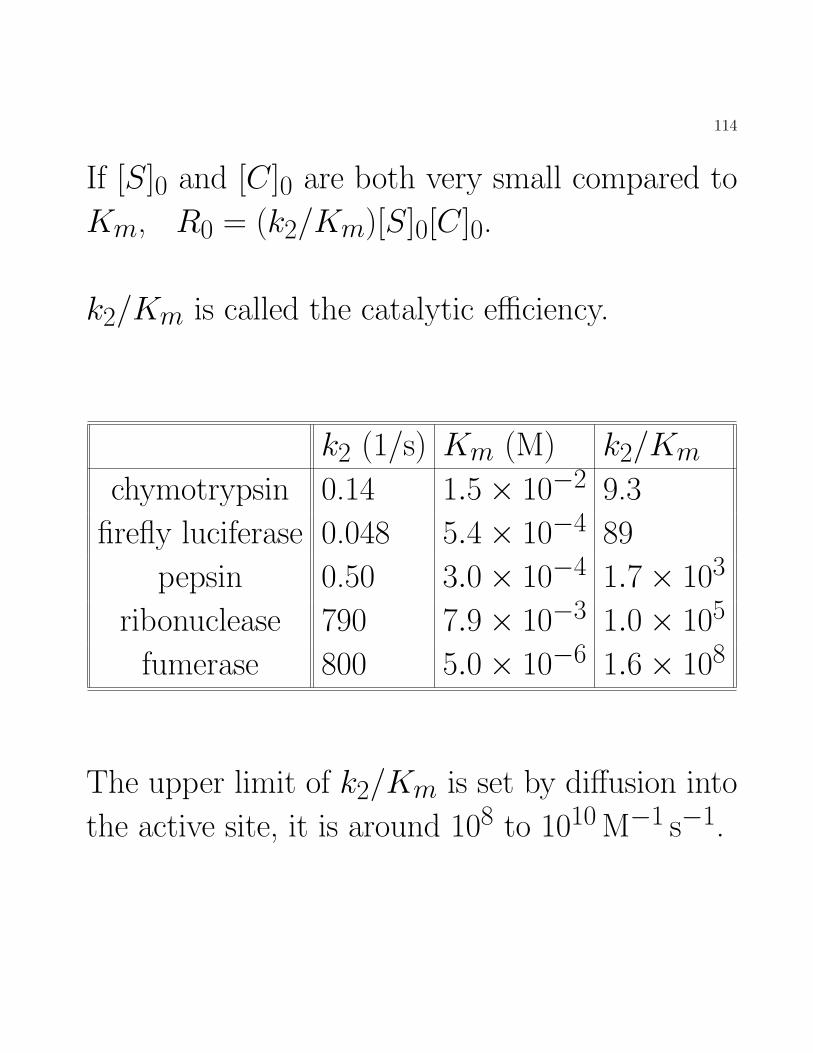
If [S]0 and [C]0 are both very small compared to
Km, R0 = (k2/Km)[S]0[C]0.
k2/Km is called the catalytic efficiency.
k2 (1/s) Km (M) k2/Km
chymotrypsin 0.14 1.5× 10⁻² 9.3
firefly luciferase 0.048 5.4× 10⁻⁴ 89
pepsin 0.50 3.0× 10⁻⁴ 1.7× 10³
ribonuclease 790 7.9× 10⁻³ 1.0× 10⁵
fumerase 800 5.0× 10⁻⁶ 1.6× 10⁸
The upper limit of k2/Km is set by diffusion into
the active site, it is around 108 to 1010 M−1 s−1.

115
A competitive inhibitor I:
• is structurally similar to S,
• binds to the same enzyme active site,
• but does not react.
With inhibitor I:
E + S � ES
ES → E + P
E + I � EI
Now [E]0 = [E] + [ES] + [EI ].
We use the PEA and assume that k2 is small,
Ks =k−1
k1=
[E][S]
[ES]≈ k−1 + k2
k1= Km
Ki =k−3
k3=
[E][I ]
[EI ]

116
Rewrite [E] and [EI ],
substitute in [E]0 = [E] + [ES] + [EI ],
and solve for [ES] . . .
. . .
Assuming [S] ≈ [S]0, the rate, R = k2[ES], is
R ≈ k2[S]0[E]0
[S]0 + Km
(1 +
[I ]Ki
)as before withKm changed toK∗m ≡ Km
(1 +
[I ]Ki
).
We also get the same equations for R0 and 1/R0,
with Km replaced by K∗m.
K∗m > Km, so R0 decreases in the presence of
an inhibitor.

117
Many metabolic regulators, drug molecules, and
poisons, are competitive inhibitors (CI).
? some CI are involved in negative feedback. They
slow down an enzymatic reaction when products
build up ⇒ homeostasis, the ability of a cell (or
an organism) to maintain stable conditions (T ,
pH, [Na+], [K+], . . . ).
? some CI drugs kill bacteria or viruses by binding
to enzymes used in their replication.
? other CI drugs correct a metabolic imbalance
by slowing down a reaction.
? protein kinase inhibitors are used in the treat-
ment of cancers and inflammations.

118
? snake venoms often contain powerful inhibitors.
The king cobra’s venom has alpha-neurotoxins that
mimick the shape of acetylcholine, bind to its re-
ceptors on motor neurons, and cause paralysis.
Research on venoms may lead to new drugs!
? snakes evolved more powerful venoms while mon-
gooses, opposums, and others evolved better resis-
tance. That’s the evolutionary arms race.
? humans evolved the phamaceutical industry . . .

119
A homogeneous catalyst is in the same phase as
the reactants and products.
A heterogeneous catalyst is in a different phase
(usually solid).
120
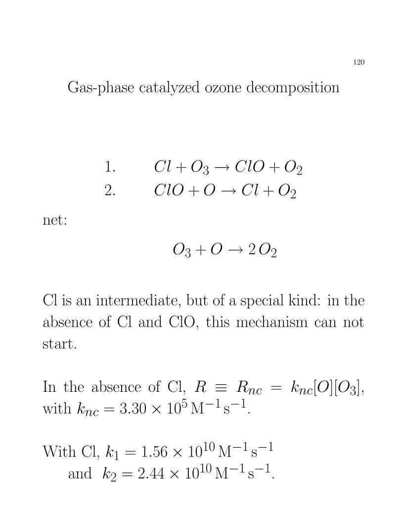
Gas-phase catalyzed ozone decomposition
1. Cl + O3→ ClO + O2
2. ClO + O → Cl + O2
net:
O3 + O → 2O2
Cl is an intermediate, but of a special kind: in the
absence of Cl and ClO, this mechanism can not
start.
In the absence of Cl, R ≡ Rnc = knc[O][O3],
with knc = 3.30× 10⁵ M−1 s−1.
With Cl, k1 = 1.56× 10¹⁰ M−1 s−1
and k2 = 2.44× 10¹⁰ M−1 s−1.

121
With the catalyzed mechanism and SSA,
d[Cl]
dt= 0 = −k1[Cl][O3] + k2[ClO][O]
[ClO] =k1[Cl][O3]
k2[O]
Then we make the SSA for the sum of intermedi-
ate concentrations:
[Cl] + [ClO] = [Cl]total
where [Cl]total is a constant. Then
[Cl] = [Cl]total −k1[Cl][O3]
k2[O]
[Cl] =[Cl]total k2 [O]
k1[O3] + k2[O]

122
The rate is
Rcat = k1[O3][Cl] =k1k2 [Cl]total [O] [O3]
k1[O3] + k2[O]
Ozone is reactive, but much less than O atoms,
so [O3] � [O] and we can neglect k2[O] in the
denominator:
Rcat = k2[Cl]total[O]

123
The ratio of ratesRcat/Rnc = k2[Cl]total/knc[O3].
Using the numerical values of k2, knc, and
[Cl]total/[O3] ≈ 10−3, we find Rcat/Rnc ≈ 74.
Elimination of anthropogenic Cl in the atmosphere
is crucial for preserving the ozone layer.
Rowland and Molina hypothesized that photolysis
of CFCl3 and CF2Cl2 (“freon”, used in old refrig-
erators and aerosols) was a major source of Cl.
These compounds are being phased out.

124
Solid catalysts
A key step is often the adsorption of gas molecules
A on a solid catalyst’s surface
A(g) + M(surface)� A ·M(surface)
M represents an adsorption site on the surface.
Assume there are N of them. The Langmuir
model assumes that:
1. At mostN molecules can adsorb on the surface.
2. All the surface sites are equivalent.
3. Adsorption and desorption at a site happens
independently of the other sites.

125
Define the coverage θ = Vads/Vm: fraction of sites
occupied by A, and P = pressure of A(g).
Vm: maximum volume of gas that can be ad-
sorbed.
dθ
dt= kaPN(1− θ)− kdNθ
At equilibrium, dθ/dt = 0 and we get
θ =kaP
kaP + kd=
KP
KP + 1
K = ka/kd. This is the Langmuir isotherm.
126
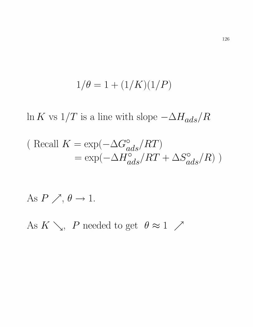
1/θ = 1 + (1/K)(1/P )
lnK vs 1/T is a line with slope −∆Hads/R
( Recall K = exp(−∆G◦ads/RT )
= exp(−∆H◦ads/RT + ∆S◦ads/R) )
As P ↗, θ → 1.
As K ↘, P needed to get θ ≈ 1 ↗

127
In dissociative chemisorption a molecule “A2”
breaks into two fragments A upon adsorption:
A2(g) + 2M(surface)→ 2A ·M(surface)
and we get a somewhat different expression for θ,
θ =(KP )1/2
1 + (KP )1/2

128
Surfaces “M(s)” are often far from uniform, and
the kinetics of reaction can be dominated by sur-
face defects:
• M vacancy
• M adatom
• steps
• kinks

129
Radical-chain reactions
Radicals (CH3·, Cl·, HO·, . . . ) are extremely re-
active.
Small amounts of R· can trigger reactions that
would not happen otherwise.
initiation steps: molecule(s) → R·
propagation steps: the “main mechanism”
termination steps: R· → molecule(s)
The propagation steps add up to the net reaction.

130
initiation 1. C2H6→ 2CH3 ·2. CH3 · + C2H6→ CH4 + C2H5·
propagation 3. C2H5· → C2H4 + H ·4. H · + C2H6→ C2H5 · +H2
termination 5. H · + C2H5· → C2H6
∆H for each step:
1: +90 kcal/mol
2: −4.3 kcal/mol
3: +36 kcal/mol
4: −3.6 kcal/mol
5: −101 kcal/mol,
steps 1 and 5 are rare events;
step 2 is “fed” CH3· by step 1 only;
steps 3 and 4 feed each other.

131
The only step where C2H4 is produced is 3., so
the rate for the overall reaction is
R = k3[C2H5·]
let R· = H·, CH3· , or C2H5·
0 ≈ d[R·]dt
= 2k1[C2H6]− 2k5[H·][C2H5·]
[H·] =k1[C2H6]
k5[C2H5·]
0 ≈ d[H·]dt
= k3[C2H5·]
−k4[C2H6]
(k1[C2H6]
k5[C2H5·]
)−k5[C2H5·]
(k1[C2H6]
k5[C2H5·]
)

132
Let x = [C2H5·] and multiply by x/k3 everywhere
0 = x2 − k1
k3[C2H6]x− k1k4
k3k5[C2H6]2
It is a quadratic equation for x with solutions
x =k1
2k3[C2H6]
±
((k1
2k3[C2H6]
)2
+k1k4
k3k5[C2H6]2
)1/2
x = [C2H6]
k1
2k3±
((k1
2k3
)2
+k1k4
k3k5
)1/2
• we keep the “+” sign, or else x < 0
• k1 is very small, so we neglect (k1/2k3)2, and

133
then neglect (k1/2k3), so all that’s left is
[C2H5·] = x =
(k1k4
k3k5
)1/2
[C2H6]
so
R = k3[C2H5·] = k3
(k1k4
k3k5
)1/2
[C2H6]
R =
(k1k3k4
k5
)1/2
[C2H6]

134
Radical-chain polymerization
We have radicals R· formed by cleavage of an ini-
tiator I , and monomers M :
initiation I → 2R · (ki)
R · +M →M1 · (k1)
propagation M1 · +M →M2 ·M2 · +M →M3 · (kp)
. . .
Mn−1 · +M →Mn ·
termination Mm · +Mn· →Mm+n · (kt)
Let [M ·] = [M1·] + [M2·] + [M3·]+ . . .
We apply the SSA to [M ·].

135
d[M ·]dt
= 2φki[I ]− 2kt[M ·]2 ≈ 0
φ is the probability that R· reacts with M, and
not with something else.
[M ·] =
(φkikt
)1/2
[I ]1/2
d[M ]
dt= −kp[M ·][M ]− (k1[R·][M ])
≈ −kp(φkikt
)1/2
[I ]1/2 [M ]
The kinetic chaing length ν is the ratio of (a)
the rate of consumption of M, to (b) the rate of
creation of M1·.

136
ν =kp[M ·][M ]
2φki[I ]
ν =kp[M ]
2(φkikt)1/2[I ]1/2
The average length of polymers ν determines the
properties of a material, and it can be controlled
by the choice of [I ].

137
Explosions
Two types of explosions:
(1) If ∆Hrxn is large and negative, and heat does
not dissipate quickly enough, T ↗, so k ↗, ge-
nerating more heat, T ↗ and k ↗, . . .
⇒ thermal explosion
(2) If radicals are produced faster than they are
consumed, their concentration increases exponen-
tially, reaction rates increase exponentially, . . .
⇒ chain-branching explosion

138
2H2(g) + O2(g)→ 2H2O(g)
1. H2 + O2→ 2OH · (+2)
2. H2 + OH· → H · +H2O (0)
3. H · +O2→ OH · + ·O · (+1)
4. ·O · +H2→ OH · +H · (+1)
5. H · +O2 + M → HO2 · +M∗ (0)
. . .

139
1. initiation: stable molecules give radicals.
2. and 5. propagation: no net change in num-
ber of radicals.
3. and 4. branching reactions: one radical in
reactants, two radicals in products.
termination steps are omitted for simplicity
Radicals produced in 3. and 4. may diffuse out of
the reaction mixture: at low P , diffusion prevents
explosion.
At high P , radical-radical recombination may pre-
vent explosion.
At intermediate P , the reaction is explosive.

140
A generic chain-branching mechanism
R·: any radical
A, B: reactants ; P1, P2: products
φ: mean number of radicals produced in bran-
ching reactions (branching efficiency)
initiation A + B → R · ki
branching R· → φR · +P1 kb
termination R· → P2 kt
141
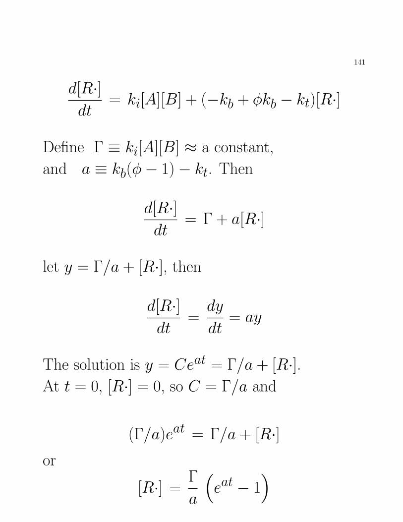
d[R·]dt
= ki[A][B] + (−kb + φkb − kt)[R·]
Define Γ ≡ ki[A][B] ≈ a constant,
and a ≡ kb(φ− 1)− kt. Then
d[R·]dt
= Γ + a[R·]
let y = Γ/a + [R·], then
d[R·]dt
=dy
dt= ay
The solution is y = Ceat = Γ/a + [R·].At t = 0, [R·] = 0, so C = Γ/a and
(Γ/a)eat = Γ/a + [R·]or
[R·] =Γ
a
(eat − 1
)

142
If kt < kb(φ − 1), then a > 0, and as t → ∞,
[R·]→∞: explosion
If kt > kb(φ − 1), then a < 0. Let a′ ≡ −a(a′ > 0), then
[R·] =Γ
a′
(1− e−a
′t)
As t → ∞, [R·] → Γ/a′. [R·] goes to a finite
limiting value: no explosion.

143
Photochemistry
Many reactions are driven by absorption of light.
One of the simplest scheme is
Ahν→ A∗→ Products
energy of a photon
Ephoton = hν = hc/λ
Beer-Lambert law:
Iabs = 2.303× I0 ε ` [A]
I0, Iabs: incident/absorbed light intensity,
in “mole of photon cm−2 s−1”
`: optical path length, in cm
ε: molar absorptivity, in M−1 cm−1
2.303 = ln 10

144
Beer’s law
A beam of light of intensity I0 goes through a homogeneous dilute solu-
tion of absorbers “A” with concentration [A]. The light gets attenuated
as it goes through the cell of length ` and exits with intensity I < I0.
We want to calculate I or Iabs = I0 − I .
Let’s say the light travels along x, with x = 0 at the entry point
into the solution, and x = ` at the exit point: ` is the path length.
At x = 0, I = I0. The probability that a photon of the beam gets
absorbed between x = 0 and x = dx is Prob∝ [A]dx or Prob= ε[A]dx,
where ε is the proportionality factor which depends on the molecule “A”
absorbing light and the wavelength λ. The attenuation factor between
x = 0 and x = dx is (1− ε[A]dx), and the intensity of light at x = dx
is
I(dx) = I0(1− ε[A]dx)
The attenuation factor is also (1− ε[A]dx) for x = dx to x = 2dx, and
for x = 2dx to x = 3dx, and so on. So
I(2dx) = I0(1− ε[A]dx)2
I(3dx) = I0(1− ε[A]dx)3
. . .
Then, I(`) ≡ I = I0(1− ε[A]dx)n, or
I0/I = (1− ε[A]dx)−n
ln(I0/I) = −n ln(1− ε[A]dx)
= −n(−ε[A]dx− (ε[A]dx)2 − . . . )

145
In the limit dx→ 0 we have
ln(I0/I) = nε[A]dx
Since n = `/dx,
ln(I0/I) = ε`[A]
Instead of I0/I or Iabs = I0 − I , people sometimes write Beer’s law in
term of the transmittance T = I/I0:
I/I0 ≡ T = e−ε`[A]
Instead of natural logarithms, people sometimes use base-10 log, and a
ε that is 2.303 times smaller:
T = 10−ε`[A] ≡ 10−A
A = ε`[A]
A is called the absorbance. The derivation of Beer’s law depends on
the assumption that [A] is sufficiently small (dilute solution). If [A] is
large, we could have A—A interactions and cooperative effects. If [A] is
small enough, we can further simplify Beer’s law:
I0/I = eε`[A]
= 1 + ε`[A] +1
2(ε`[A])2 + . . .
Keeping only the first two terms,
I0/I ≈ I/I + ε`[A]
I0 − I ≈ Iε`[A]
146
When [A] is very small, we normally have I/I0 ≈ 1 and we can write
Iabs = I0 − I like this
I0 − I ≡ Iabs ≈ I0ε`[A]
or, if we use the log10 convention instead,
Iabs ≈ 2.303× I0ε`[A]
with ε smaller by a factor 2.303.

147
The rate of photoexcitation R =d[A∗]dt = −d[A]
dt ,
in M s−1, is
R =Iabs`× 1000 cm3/L
so
−d[A]
dt= 2303 I0 ε [A]
After integration,
[A] = [A]0 e−2303I0εt
This describes the kinetics of many first-order pho-
tochemical reactions.
Working with number of molecules “A” andNA =
6.022 × 10²³mol−1 instead of concentration [A],
we have . . .

148
−dAdt
=2303I0ε
NAA
A = A0 e−I0(2303ε/NA)t
A = A0 e−I0σAt
NOTE: now I0 is in “photon cm−2 s−1”.
σA has units cm3
L ×M−1 cm−1
mol−1 = cm2 and is
called the absorption cross section.
ka = I0σA is in cm−2 s−1 cm2, or s−1.
A = A0e−kat

149
Jablonski diagram

150
wiggly lines: vibrational relaxation (vr)
horizontal lines:
S1 to S0: internal conversion (ic)
S1 to T1: intersystem crossing (isc) “S”
T1 to S0: isc “T”
vertical lines:
S0 to S1: photon absorption
S1 to S0: fluorescence (photon emission)
T1 to S0: phosphorescence (photon emission)

151
Most molecules have a closed-shell electronic ground
state, and most electronic excitations can be viewed
as promoting a single electron. This leads to 4 spin
configurations for the excited states.
α(s1)β(s2) ≡ αβ, β(s1)α(s2) ≡ βα,
α(s1)α(s2) ≡ αα, and β(s1)β(s2) ≡ ββ.
The 4 correct spin functions are:
1√2(αβ − βα): one state S1
1√2(αβ + βα), αα, and ββ: a triplet of states T1
152
Each process has an associated rate constant.
kvr ≈ 1013 s−1 is very big. We assume that vi-
brational relaxation is instantaneous.
The rates of the other processes are:
S1 to S0 + hν, fluorescence: kf [S1]
T1 to S0 + hν, phosporescence: kp[T1]
S1 to T1, isc: kisc,S[S1]
S1 to S0, ic: kic[S1]
T1 to S0, isc: kisc,T [T1]

153
Excited molecules in state S1 can return to the
ground state by collisional quenching:
S1 + Q→ S0 + Q
with rate
Rq = kq [S1][Q]
Accounting for all processes involving S1 and ma-
king the SSA,
0 ≈ ka[S0]− [S1](kf + kic + kisc,S + kq[Q])
The fluorescence lifetime is
1
τf= kf + kic + kisc,S + kq[Q]
Then
[S1] = ka[S0] τf

154
The fluorescence intensity is
If = kf [S1] = ka kfτf [S0] = kaΦf [S0]
Φf =kf
kf+kic+kisc,S+kq[Q]is the quantum yield
for fluorescence — the fraction of molecules in S1
that return to the ground state by fluorescing.
Molecules that emit strongly often have kf � kicand kf � kisc,S. Then
1
If≈ 1
ka[S0]+
kqkakf [S0]
[Q]
I0
If= 1 +
kqkf
[Q]
I0If
vs [Q] is a Stern-Volmer (SV) plot.

155
O2 and acrylamide (CH2CHCONH2) are common
quenchers.
SV plots have been used to measure the acces-
sibility of tryptophan residues in proteins
⇒ conformation, ∼ 10−10 s dynamics
W Qiu et al., Chemical Physics 350 (2008) 154–
164.
156
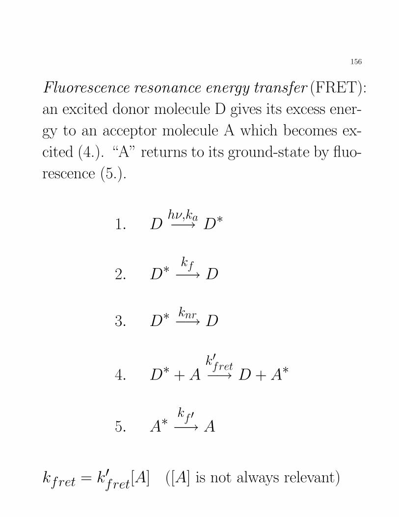
Fluorescence resonance energy transfer (FRET):
an excited donor molecule D gives its excess ener-
gy to an acceptor molecule A which becomes ex-
cited (4.). “A” returns to its ground-state by fluo-
rescence (5.).
1. Dhν,ka−→ D∗
2. D∗kf−→ D
3. D∗knr−→ D
4. D∗ + Ak′fret−→ D + A∗
5. A∗kf ′−→ A
kfret = k′fret[A] ([A] is not always relevant)

157
From the viewpoint of D∗, FRET is one more non-
radiative (nr) process for returning to the ground
state, in addition to ic, ics, and quenching, so
Φf =kf
kf + knr
knr = kic + kics,S + kq[Q]
becomes
Φf,fret =kf
kf + knr + kfret
The quantum yield for FRET is
Φfret =kfret
kf + knr + kfret
(Φfret is “Eff” in the book, equation (19.179))

158
In practice Φfret is measured by the difference in
the fluorescence of D in the presence of A
Φfret = 1−Φf,fret
Φf
The probability of energy transfer, Φfret, is very
sensitive to the D-A separation “r”.
Φfret =1
1 + (r/r0)6
r0 depends on the D/A pair and is normally be-
tween 10 and 60 A.
A FRET signal tells us that D and A are close.
159
Ex. 1: we label a membrane receptor with D,
and a ligand with A. We see a FRET signal and
conclude that the ligand binds to the receptor.
Ex. 2: we label two sites of a biomolecule with
D and A. At pH 7.4, we see a FRET signal; at
pH 5.0 we see no FRET. We conclude that the
biomolecule underwent a conformational change.
160
For FRET to occur, r/r0 must be small enough.
In order to have a sizeable r0,
• D should have a large Φf ,
• the absorption band of A and fluorescence band
of D should overlap,
• and the transition dipoles of D and A should
be aligned, at least some of the time.
FRET is essential for photosynthesis
A FRET-based heterojunction has been proposed
for use in solar cells, see Nature Photonics 7 (2013)
479-485.

161
Photochemical reactions: a photoexcited molecule,
usually in S1 reacts at a rate
Rphotochem. = kphoto,S1[S1]
Quantum yield
φ =kphoto,S1
kf + knr + kphoto,S1
φ: fraction of excited molecules that react
Number of absorbed photons, Nabs
Nabs =Eabs
Ephoton=P∆t
hν=P∆t
hc/λ
P : power (in Watts, W)

162
Electron transfer
D + A� D+ + A−
essential in photovoltaics & photosynthesis
6CO2(g) + 6H2O(`)→ C6H12O6(s) + 6O2(g)
∆G◦ = 2870 kJ: reaction driven by light.
• light absorption
• FRET (energy migration to rxn center)
• e− transfer reactions
• many other reactions
163
e− transfer kinetics
The donor D and acceptor A diffuse and form a
complex, transfer an e−, and separate.
D + A� DA (kd, k′d)
DA� D+A− (ke, k′e)
D+A−→ D+ + A− (ksep)
SSA for [D+A−]:
[D+A−] =ke[DA]
k′e + ksep

164
SSA for [DA]:
[DA] =kd[D][A] + k′e[D
+A−]
k′d + ke
Substituting:
[D+A−] =kekd
k′ek′d + ksepk′d + ksepke
[D][A]
the rate is
R = ksep[D+A−] = k[D][A]
We assume ksep� k′e, so
R =kekdke + k′d
[D][A]

165
Two limiting cases:
1) ke� k′d: R = kd[D][A] (diffusion controlled)
2) ke� k′d: R = keKd[D][A] (Kd = kd/k′d)
case 2. applies when D and A are bonded, or held
together by a surrounding protein(s).

166
A microscopic view of e− transfer:
Marcus theory (∼ 1956)
e− transfer between D and A occurs if . . .
orbitals overlap: k ∝ e−βr
D and A have sufficient energy to overcome an
activation barrier: k ∝ e−∆G‡/kBT
∆G◦: free energy change for the charge transfer
λ > 0: reorganization energy, free energy of DA
at the equilibrium geometry of D+A−, including
the solvent.
∆G‡ =(∆G◦ + λ)2
4λ
167
x: reaction coordinate
x = 0, equilibrium geometry of DA;
x = a, equilibrium geometry of D+A−
Assume the free energies of DA (Gn) and D+A−
(Gt) are quadratic wrt displacement from equili-
brium, with force constant k, and set ∆G = 0 at
x = 0.
Gn =1
2kx2
Gt =1
2k(x− a)2 + ∆G◦
=1
2k(x2 − 2ax + a2) + ∆G◦

168
The two energy curves cross at xc:
1
2kx2
c =1
2k(x2
c − 2axc + a2) + ∆G◦
kaxc =1
2ka2 + ∆G◦
λ = 12 ka
2, so
kaxc = ∆G◦ + λ
xc =∆G◦ + λ
kaEnergy at xc:
∆G‡ =1
2kx2
c =k
2
(∆G◦ + λ
ka
)2
=(∆G◦ + λ)2
2ka2
∆G‡ =(∆G◦ + λ)2
4λ

169
• k ∝ e−βr e−∆G‡/kBT ∝ Ae−∆G‡/kBT
same form as Eyring’s formula
• the rate is maximum at ∆G◦ = −λ
• ∆G◦ < −λ: “inverted regime” (expt in 1984)
• e− transfer can be accompanied by an impor-
tant solvent reorganization, and large λ
• “outer sphere” reactions: only the solvent reor-
ganizes. The e− transfers when the solvation shell
is optimal for stabilizing a fictitious D+qA−q.
• ∆G◦ generally more negative in polar solvents
• applications: photosynthesis, corrosion, chemi-
luminescence, solar cells

170
Rudolph Marcus:
PhD McGill 1946
postdoc at NRC, Ottawa 1946-49
UNC Chapel Hill, 1949-51
prof at Brooklyn Polytechnic,
U Illinois Urbana-Champaign,
Caltech
Recommended