CE
E 3
20S
pri
ng
200
7
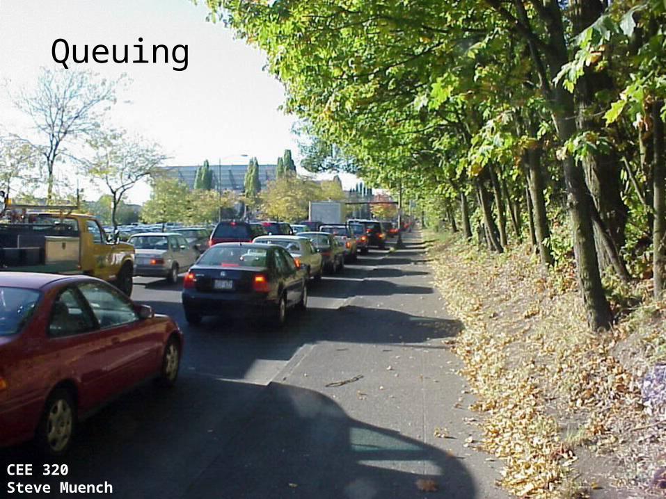
Queuing
CEE 320Steve Muench
CE
E 3
20S
pri
ng
200
7
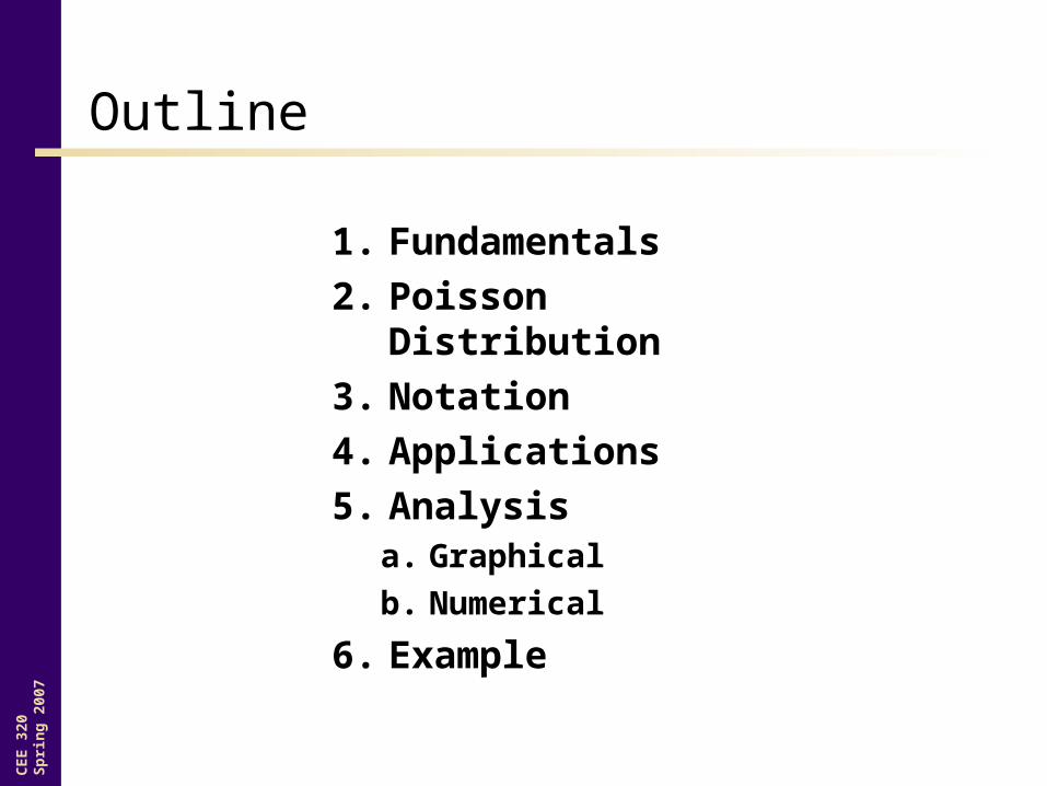
Outline
1. Fundamentals
2. Poisson Distribution
3. Notation
4. Applications
5. Analysisa. Graphical
b. Numerical
6. Example

CE
E 3
20S
pri
ng
200
7
Fundamentals of Queuing Theory
• Microscopic traffic flow
• Arrivals– Uniform or random
• Departures– Uniform or random
• Service rate– Departure channels
• Discipline– FIFO and LIFO are most popular– FIFO is more prevalent in traffic engineering

CE
E 3
20S
pri
ng
200
7
Poisson Distribution
• Count distribution– Uses discrete values– Different than a continuous distribution
!n
etnP
tn
P(n) = probability of exactly n vehicles arriving over time t
n = number of vehicles arriving over time t
λ = average arrival rate
t = duration of time over which vehicles are counted
CE
E 3
20S
pri
ng
200
7
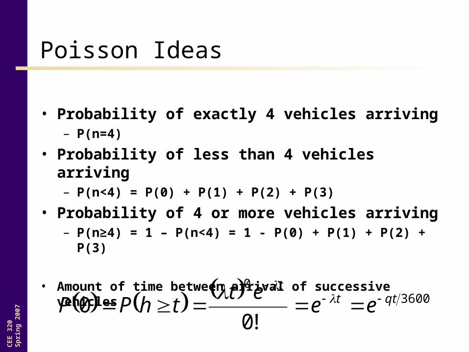
Poisson Ideas
• Probability of exactly 4 vehicles arriving– P(n=4)
• Probability of less than 4 vehicles arriving– P(n<4) = P(0) + P(1) + P(2) + P(3)
• Probability of 4 or more vehicles arriving– P(n≥4) = 1 – P(n<4) = 1 - P(0) + P(1) + P(2) + P(3)
• Amount of time between arrival of successive vehicles
36000
!00 qtt
t
eeet
thPP
CE
E 3
20S
pri
ng
200
7
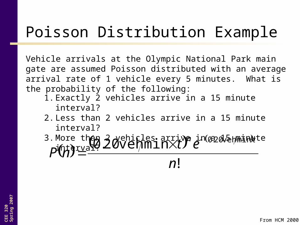
Poisson Distribution Example
From HCM 2000
Vehicle arrivals at the Olympic National Park main gate are assumed Poisson distributed with an average arrival rate of 1 vehicle every 5 minutes. What is the probability of the following:
1. Exactly 2 vehicles arrive in a 15 minute interval?2. Less than 2 vehicles arrive in a 15 minute interval?3. More than 2 vehicles arrive in a 15 minute interval?
!
minveh20.0 minveh20.0
n
etnP
tn

CE
E 3
20S
pri
ng
200
7
Example Calculations
%4.22224.0
!2
1520.02
1520.02
e
PExactly 2:
Less than 2:
More than 2:
102 PPnP
21012 PPPnP
CE
E 3
20S
pri
ng
200
7
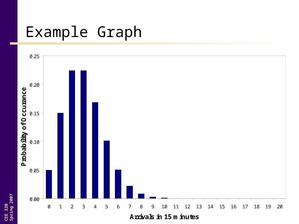
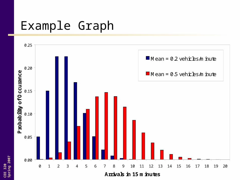
Example Graph
0.00
0.05
0.10
0.15
0.20
0.25
0 1 2 3 4 5 6 7 8 9 10 11 12 13 14 15 16 17 18 19 20
Arrivals in 15 minutes
Pro
bab
ilit
y o
f O
ccu
ran
ce
CE
E 3
20S
pri
ng
200
7 0.00
0.05
0.10
0.15
0.20
0.25
0 1 2 3 4 5 6 7 8 9 10 11 12 13 14 15 16 17 18 19 20
Arrivals in 15 minutes
Pro
bab
ilit
y o
f O
ccu
ran
ce
Mean = 0.2 vehicles/minute
Mean = 0.5 vehicles/minute
Example Graph
CE
E 3
20S
pri
ng
200
7
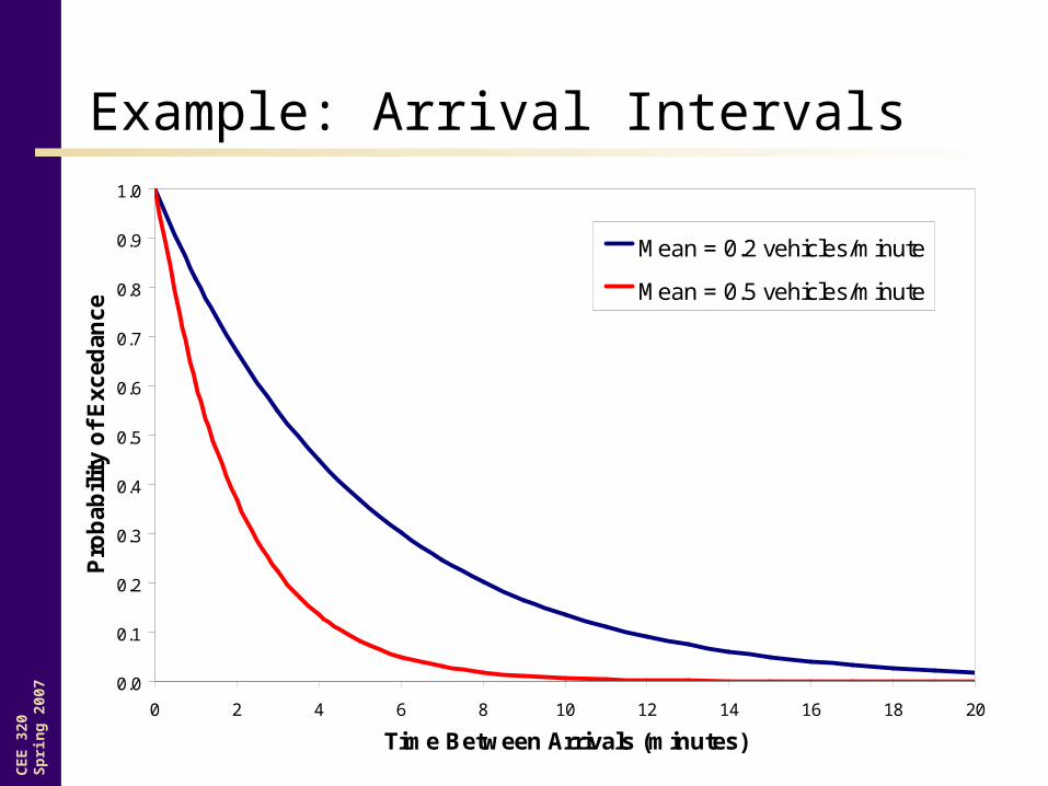
Example: Arrival Intervals
0.0
0.1
0.2
0.3
0.4
0.5
0.6
0.7
0.8
0.9
1.0
0 2 4 6 8 10 12 14 16 18 20
Time Between Arrivals (minutes)
Pro
bab
ilit
y o
f E
xced
ance
Mean = 0.2 vehicles/minute
Mean = 0.5 vehicles/minute
CE
E 3
20S
pri
ng
200
7
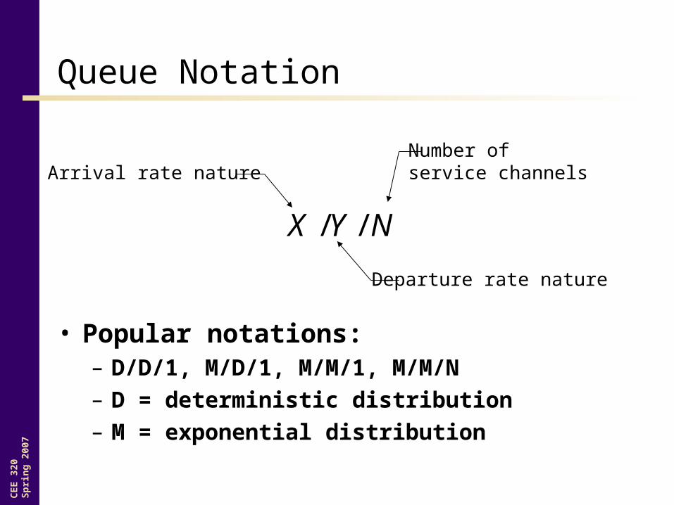
Queue Notation
• Popular notations:– D/D/1, M/D/1, M/M/1, M/M/N– D = deterministic distribution– M = exponential distribution
NYX //
Arrival rate nature
Departure rate nature
Number ofservice channels
CE
E 3
20S
pri
ng
200
7
Queuing Theory Applications• D/D/1
– Use only when absolutely sure that both arrivals and departures are deterministic
• M/D/1 – Controls unaffected by neighboring controls
• M/M/1 or M/M/N– General case
• Factors that could affect your analysis:– Neighboring system (system of signals)– Time-dependent variations in arrivals and departures
• Peak hour effects in traffic volumes, human service rate changes
– Breakdown in discipline• People jumping queues! More than one vehicle in a lane!
– Time-dependent service channel variations• Grocery store counter lines

CE
E 3
20S
pri
ng
200
7
Queue Analysis – Graphical
ArrivalRate
DepartureRate
Time
Ve
hicl
es
t1
Queue at time, t1
Maximum delay
Maximum queue
D/D/1 Queue
Delay of nth arriving vehicle
Total vehicle delay
CE
E 3
20S
pri
ng
200
7
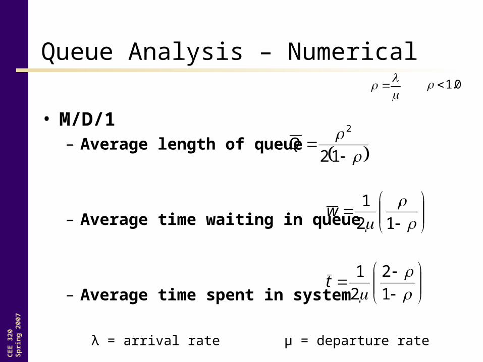
Queue Analysis – Numerical
• M/D/1– Average length of queue
– Average time waiting in queue
– Average time spent in system
0.1
12
2
Q
12
1w
1
2
2
1t
λ = arrival rate μ = departure rate
CE
E 3
20S
pri
ng
200
7
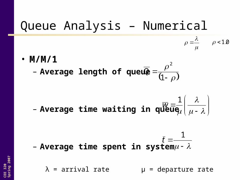
Queue Analysis – Numerical
• M/M/1– Average length of queue
– Average time waiting in queue
– Average time spent in system
0.1
1
2
Q
1
w
1t
λ = arrival rate μ = departure rate

CE
E 3
20S
pri
ng
200
7
Queue Analysis – Numerical
• M/M/N– Average length of queue
– Average time waiting in queue
– Average time spent in system
2
10
1
1
! NNN
PQ
N
1
Q
w
Q
t
0.1N
λ = arrival rate μ = departure rate
CE
E 3
20S
pri
ng
200
7
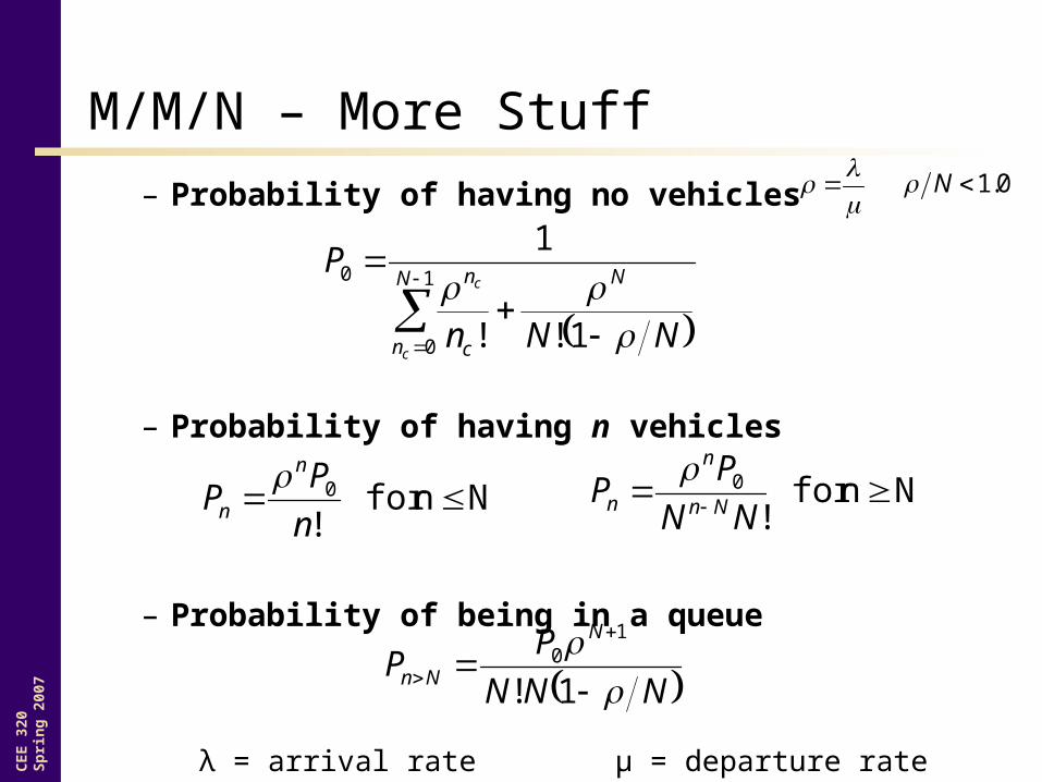
M/M/N – More Stuff
– Probability of having no vehicles
– Probability of having n vehicles
– Probability of being in a queue
1
0
0
1!!
1N
n
N
c
n
c
c
NNn
P
Nnfor !
0 n
PP
n
n
Nnfor !
0 NN
PP
Nn
n
n
NNN
PP
N
Nn
1!
10
0.1N
λ = arrival rate μ = departure rate
CE
E 3
20S
pri
ng
200
7
Example 1
You are entering Bank of America Arena at Hec Edmunson Pavilion to watch a basketball game. There is only one ticket line to purchase tickets. Each ticket purchase takes an average of 18 seconds. The average arrival rate is 3 persons/minute.
Find the average length of queue and average waiting time in queue assuming M/M/1 queuing.
CE
E 3
20S
pri
ng
200
7
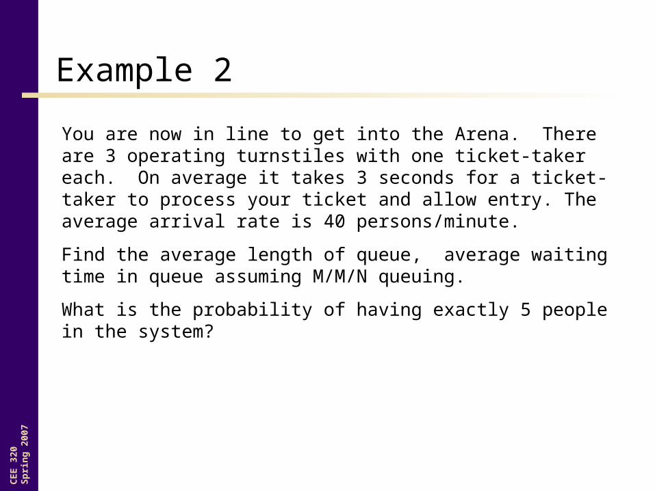
Example 2
You are now in line to get into the Arena. There are 3 operating turnstiles with one ticket-taker each. On average it takes 3 seconds for a ticket-taker to process your ticket and allow entry. The average arrival rate is 40 persons/minute.
Find the average length of queue, average waiting time in queue assuming M/M/N queuing.
What is the probability of having exactly 5 people in the system?
CE
E 3
20S
pri
ng
200
7
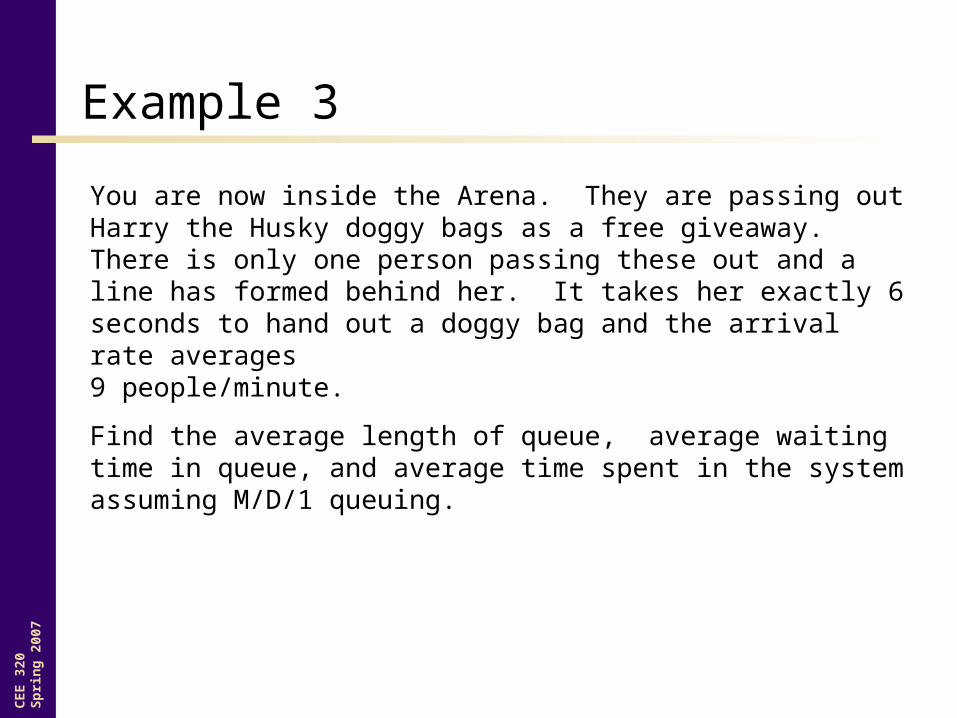
Example 3
You are now inside the Arena. They are passing out Harry the Husky doggy bags as a free giveaway. There is only one person passing these out and a line has formed behind her. It takes her exactly 6 seconds to hand out a doggy bag and the arrival rate averages 9 people/minute.
Find the average length of queue, average waiting time in queue, and average time spent in the system assuming M/D/1 queuing.
CE
E 3
20S
pri
ng
200
7
Primary References
• Mannering, F.L.; Kilareski, W.P. and Washburn, S.S. (2003). Principles of Highway Engineering and Traffic Analysis, Third Edition (Draft). Chapter 5
• Transportation Research Board. (2000). Highway Capacity Manual 2000. National Research Council, Washington, D.C.
Recommended