Brian KinlanUC Santa Barbara
Integral-difference model simulations of marine population genetics

Population genetic structure
-Analytical models date back to Fisher, Wright, Malecot 1930’s -1950’s
-Neutral theory
-Can give insight into population history and demography
-Many simplifying assumptions
-One of the most troublesome – Equilibrium
-Simulations to understand real data?

Glossary
Allele
Locus
Heterozygosity
Polymorphism
Deme
Marker (e.g., Allozyme, Microsatellite, mtDNA)
Hardy-Weinberg Equilibrium
Genetic Drift
Many possible inferences
-Effective population size
-Inbreeding/selfing
-Mating success
-Bottlenecks
-Time of isolation
-Migration/dispersal
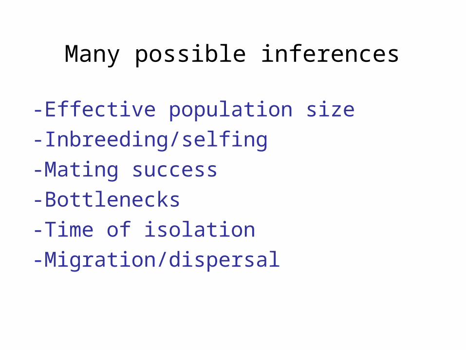
Many possible inferences
-Effective population size
-Inbreeding/selfing
-Mating success
-Bottlenecks
-Time of isolation
-Migration/dispersal

Population structure
vs.
t=0; no structuret=500; structure

Avg Dispersal = 10 km; Domain = 1000 km; Spacing = 5 km; 1000 generations; Ne=100
Population structure

Measuring population structure
-F statistics – standardized variance in allele frequencies among different population components (e.g., individual-to-subpopulation; subpopulation-to-total)
-Other measures (assignment tests, AMOVA, Hierarchical F, IBD, Genetic Distances, Moran’s I, etc etc etc)
-For more http://genetics.nbii.gov/population.html
http://dorakmt.tripod.com/genetics/popgen.html

Heterozygosity
-Hardy-Weinberg Equilibrium (well-mixed):
1 locus, 2 alleles, freq(1)=p, freq(2)=q
HWE => p2 + 2pq +q2
-Deviations from HWEDeviations of observed frequency of heterozygotes (Hobs) from those expected under HWE (Hexp) can occur due to non-random mating and sub-population structure

FF = fixation index and is a measure of how much theobserved heterozygosity deviates from HWE
F = (He - Ho)/He
HIHI = observed heterozygosity over ALL subpopulations.
HIHI = (Hi)/k where Hi is the observed H ofthe ith supopulation and k = number ofsubpopulations sampled.
F statistics

HHSS = Average expected heterozygosity withineach subpopulation.
HS = (HIs)/k
Where HIs is the expected H within the ithsubpopulation and is equal to 1 - pi
2 wherepi
2 is the frequency of each allele.
F statistics
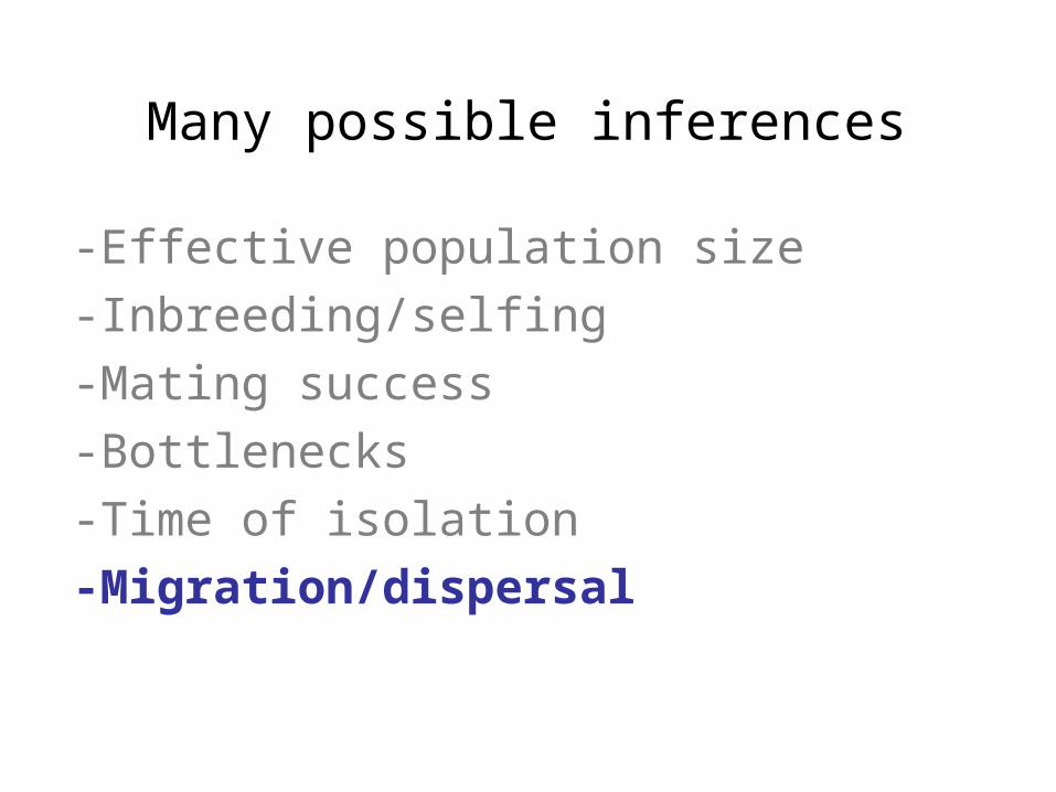
HHTT = Expected heterozygosity within the totalpopulation.
HT = 1 - xi2
where xi2 is the frequency of each allele averaged
over ALL subpopulations.
FFITIT measures the overall deviations from HWEtaking into account factors acting withinsubpopulations and population subdivision.
F statistics

FFITIT = (HT - HI)/HT and ranges from - 1 to +1because factors acting within subpopulationscan either increase or decrease Ho relativeto HWE.
Large negative values indicate overdominanceselection or outbreeding (Ho > He).
Large positive values indicate inbreeding orgenetic differentiation among subpopulations(Ho < He).
F statistics

FFISIS measures deviations from HWE withinsubpopulations taking into account only thosefactors acting within subpopulations
FFISIS = (HS - HI)/HS and ranges from -1 to +1
Positive FIS values indicate inbreeding ormating occurring among closely related individuals more often than expected underrandom mating.
Individuals will possess a large proportion ofthe same alleles due to common ancestry.

FFSTST measures the degree of differentiation among subpopulations -- possibly due to populationsubdivision.
FST = (HT - HS)/HT and ranges from 0 to 1.
FST estimates this differentiation by comparingHe within subpopulations to He in the totalpopulation.
FST will always be positive because He insubpopulations can never be greater than He inthe total population.
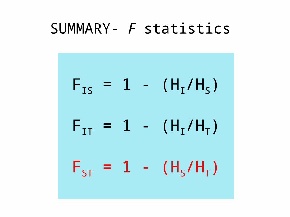
FIS = 1 - (HI/HS)
FIT = 1 - (HI/HT)
FST = 1 - (HS/HT)
SUMMARY- F statistics

Fst and Migration(Wright’s Island Model)
Fst = 1/(1+4Nm)
Nm = ¼ (1-Fst)/Fst

Limitations
I. Assumptions must be used to estimate Nm from Fst
For strict Island Model these include:
1. An infinite number of populations 2. m is equal among all pairs of populations 3. There is no selection or mutation 4. There is an equilibrium between drift and migration
“Fantasy Island?”
Other models include 1D and 2D “stepping stones”, but these too have limitations, such as a highly restrictive definition of dispersal and assumption of an infinite number of demes or a circular/toroidal arrangement.

Limitations
II. Many factors besides migration can affect Fst at any given point in space and time
-Bottlenecks-Inbreeding/asexual reproduction-Non-equilibrium-Patchiness/geometry of gene flow-Definition of subpopulations-Dispersal barriers-Cryptic speciation

Lag Distance
Sta
nd
ard
ized
Var
ian
ce
Am
on
g P
op
ula
tio
ns
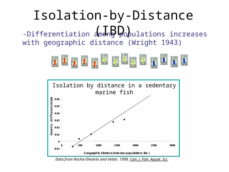
-Differentiation among populations increases with geographic distance (Wright 1943)
Isolation-by-Distance (IBD)

A dynamic equilibrium A dynamic equilibrium between drift and migrationbetween drift and migration
-Differentiation among populations increases with geographic distance (Wright 1943)
Isolation-by-Distance (IBD)
Data from Rocha-Olivares and Vetter, 1999, Can. J. Fish. Aquat. Sci.
-0.01
0
0.01
0.02
0.03
0.04
0.05
0.06
0.07
0.08
0 500 1000 1500 2000 2500 3000
Geographic distance between populations (km)
Gen
etic
dif
fere
nti
atio
n (
FS
T)
Isolation by distance in a sedentary marine fish

Calibrating the IBD Slope to Measure Dispersal
Palumbi 2003 (Ecol. App.)
-Simulations can predict the isolation-by-distance slope expected for a given average dispersal distance (Palumbi 2003 Ecol. Appl., Kinlan and Gaines 2003 Ecology)

Palumbi 2003 - Simulation Assumptions
Palumbi, 2003, Ecol. App.
1. Kernel
3. Effective population size
2. Gene flow model
Ne = 1000 per deme
Linear array of subpopulations
Pro
bab
ility
of
dis
per
sal
Distance from source
Laplacian

Kinlan & Gaines (2003) Ecology 84(8):2007-2020
Genetic Estimates of Dispersal from IBD

Siegel et al. 2003 (MEPS 260:83-96)
r2 = 0.802, p<0.001n=32
Planktonic Larval Duration (days)
Gen
eti
c D
isp
ers
al S
cale
(k
m)

Dispersal Scale vs. Developmental ModeDispersal Scale vs. Developmental ModeINVERTEBRATESINVERTEBRATES
0
20
40
60
80
100
120
140
P L N
Developmental Mode
Dis
pers
al S
cale
(km
)
Planktotrophic Lecithotrophic Non-planktonic
n=29 n=6 n=13

Genetic Dispersion Scale (km)
Mod
ele
d D
isp
ers
ion
Sca
le,
Dd
(km
)
From Siegel, Kinlan, Gaylord & Gaines 2003 (MEPS 260:83-96)

But how well do these results But how well do these results hold up to the variability and hold up to the variability and complexity of the real-world complexity of the real-world
marine environment?marine environment?

Goal: a more realistic and Goal: a more realistic and flexible population genetic modelflexible population genetic model
-Explicit modeling of population -Explicit modeling of population dynamics & dispersaldynamics & dispersal

Integro-difference model of population dynamics
A Adult abundance [#/km]
M Natural mortality
H Harvest mortality
F Fecundity
P Larval mortality
L Post - settlement recruitment
K Dispersion kernel
xt
x
x'
x
x x'
[spawners / adult]
[larvae / spawner]
[adult / settler]
[(settler / km) / total settled larvae]
A 1 M A A F K L dxxt 1
xt
xt
x x x x
( ) '' ' '
A Adult abundance [#/km]
M Natural mortality
F Fecundity
K Dispersion kernel
xt
x'
x x'
[spawners / adult]
[(settler / km) / total settled larvae]
L Post - settlement recruitmentx [adult / settler]
(Ricker form L(x) e-CA(x))

Genotypic structure (tracked somewhat analagously to age structure)

Initial Questions
-What does the approach to equilibrium look like? What is effect of non-equilibrium on dispersal estimates?
-Effects of range edges/range size
-Effects of temporal and spatial variation in demography (disturbance; spatial heterogeneity)
-Effects of flow
-How does the IBD signal “average” dispersal when the scale/pattern of dispersal is variable across the range?

Model FeaturesModel Features
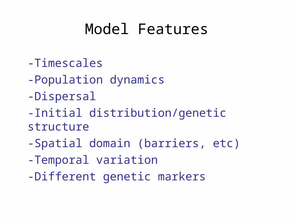
Model Features
-Timescales
-Population dynamics
-Dispersal
-Initial distribution/genetic structure
-Spatial domain (barriers, etc)
-Temporal variation
-Different genetic markers

Avg Dispersal = 12 km; Domain = 1000 km; Spacing = 5 km; 1000 generations; Ne=100
An example run

Avg Dispersal = 10 km; Domain = 1000 km; Spacing = 5 km; 1000 generations; Ne=100
t=20
t=200
t=1000

Avg Dispersal = 12 km; Domain = 1000 km; Spacing = 5 km; 1000 generations; Ne=100
Palumbi model prediction
Dd= 12.6 km

Avg Dispersal = 12 km; Domain = 1000 km; Spacing = 5 km; 1000 generations; Ne=100
Palumbi model prediction
Dd= 38 km

Avg Dispersal = 2 km; Domain = 100 km; Spacing = 5 km; 800 generations; Ne=100
t=20
t=400
t=800

Avg Dispersal = 2 km; Domain = 100 km; Spacing = 5 km; 800 generations; Ne=100
t=20
t=400
t=800Palumbi model prediction
Dd= 1.6 km

-100 -50 0 50 100 150 200 250 300 3500
0.2
0.4
0.6
0.8
1
1.2
1.4
1.6
1.8
2
U = 5 Ustd = 15 To = 14 T
f = 21
tota
l set
tlers
= 1
3 t
otal
par
t =
100
alongcoast (km)
Next stepsNext steps -Spiky kernels?Spiky kernels?-Fishing effects?Fishing effects?
-MPA’s?MPA’s?
Recommended