Bivariate Gamma Mixture of Experts Models for Joint Insurance
Claims Modeling
Sen Hu, T. Brendan Murphy, Adrian O’Hagan
School of Mathematics and Statistics, University College Dublin, Ireland
Insight Centre for Data Analytics, Dublin, Ireland
April 10, 2019
Abstract
In general insurance, risks from different categories are often modeled independently and their
sum is regarded as the total risk the insurer takes on in exchange for a premium. The dependence
from multiple risks is generally neglected even when correlation could exist, for example a single
car accident may result in claims from multiple risk categories. It is desirable to take the covariance
of different categories into consideration in modeling in order to better predict future claims and
hence allow greater accuracy in ratemaking. In this work multivariate severity models are investi-
gated using mixture of experts models with bivariate gamma distributions, where the dependence
structure is modeled directly using a GLM framework, and covariates can be placed in both gating
and expert networks. Furthermore, parsimonious parameterisations are considered, which leads
to a family of bivariate gamma mixture of experts models. It can be viewed as a model-based
clustering approach that clusters policyholders into sub-groups with different dependencies, and
the parameters of the mixture models are dependent on the covariates. Clustering is shown to be
important in separating the data into sub-groupings where strong dependence is often present, even
if the overall data set exhibits only weak dependence. In doing so, the correlation within different
components features prominently in the model. It is shown that, by applying to both simulated
data and a real-world Irish GI insurer data set, claim predictions can be improved.
Keywords: A priori ratemaking; Bivariate gamma distribution; EM algorithm; General insurance
claim modeling; Generalized linear model; Model-based clustering; Mixture of experts model.
1 Introduction
In general insurance (GI), it is a common phenomenon that claims from multiple risk categories
are correlated: in personal motor insurance an accident can lead to claims for the policyholder’s
own vehicle as well as property damage to others and bodily injury. Dependence can also be present
across multiple product lines: claim history and personal characteristics from a motor policy may
reflect information pertaining to one’s likely home policy claims. Many current insurance pricing
approaches assume independence among multiple categories, focusing on independent modeling,
and then the sum of the risks is designated as the total risk the insurer is taking on.
General linear models (GLMs) (Nelder & Wedderburn, 1972) have become the industry’s stan-
dard approach for claim modeling, typically using a univariate Poisson distribution with a log link
for the frequency aspect of modeling (how many claims are made from policies) and a univariate
gamma distribution with a log link for severity (expected size of loss for an insurer given a claim
1
arX
iv:1
904.
0469
9v1
[st
at.A
P] 9
Apr
201
9

has been made). Therefore, modeling multiple risks simultaneously using multivariate Poisson dis-
tributions (with Poisson univariate margins) and multivariate gamma distributions (with gamma
univariate margins) within the GLM framework provides a natural and useful extension beyond
their univariate counterparts. Many attempts have been made to use (finite mixtures of) multi-
variate Poisson regressions in the literature. For example, Karlis & Ntzoufras (2003) and Karlis &
Meligkotsidou (2005) investigated bivariate Poisson regressions, and Karlis & Meligkotsidou (2007)
investigated model-based clustering with finite mixtures of multivariate Poisson distributions. In
particular, Bermudez & Karlis (2012) looked at finite mixtures of bivariate Poisson regressions in
the application of GI a-priori ratemaking. However, the use of bivariate or multivariate gamma dis-
tributions has received less attention in the past, especially for GLMs and mixtures of regressions.
Hence it will be the main focus of this article, investigating the question of how multiple claim
sizes relate to each other when multiple claims are made simultaneously, with general applications
to any positive continuous data.
In recent years many studies have been carried out in the actuarial literature on multivariate
models in various insurance contexts for positive continuous data, but mainly for distribution es-
timation or risk capital analysis. For example, multivariate normal distributions (Panjer, 2002),
multivariate Tweedie distributions (Furman & Landsman, 2008; Furman & Landsman, 2010), mul-
tivariate Pareto distributions (Chiragiev & Landsman, 2007; Asimit et al., 2010) and multivariate
mixed Erlang distributions (Lee & Lin, 2012; Willmot & Woo, 2015). Multivariate gamma distri-
butions have also been studied for in the same context, see Furman & Landsman (2005), Furman &
Landsman (2010) and Furman (2008). Note that, since there are various definitions of multivariate
gamma distributions, the versions used in the literature sometimes have been defined differently.
However, none of them are studied in a regression context or a mixture model context for a-priori
insurance ratemaking. In recent years, the use of copulas has become a popular strategy for multi-
variate modeling in insurance and statistics, including ratemaking, see Frees & Valdez (1998) and
Frees et al. (2016). An advantage of the copula approach is that it uses a two stage procedure that
models the marginal distributions and a copula function (which captures the dependence structure)
separately, so it can make use of the rich resources of univariate modeling. However, this particular
feature also implies the shortcomings of copulas including estimation issues. For more detailed
discussions, see Mikosch (2006), Lee & Lin (2012) and Grazian & Liseo (2015).
In most univariate GI ratemaking models, frequency and severity are assumed to be independent.
Therefore, multivariate severity models serve an important purpose for multivariate ratemaking.
For example, a more serious car crash incident may lead the policyholder to make higher claim
sizes in multiple risk categories, given claims have been made on multiple categories. Furthermore,
some policyholders are more prone to making multiple claims but the claim sizes are usually small,
compared to other policyholders who represent higher risks, which could suggest heterogeneity in
the policy portfolio. The heterogeneity of risk could also be caused by different driving behaviours
and attitudes of the policyholders. By identifying high risk customers it is also possible to develop
further cross-selling approaches in insurance marketing. One main issue caused by heterogeneity
is that the bivariate claims data are usually very dispersed, hence data may only present a very
weak correlation overall, which could be used as justification for implementing univariate modeling
without considering dependencies among risks. It could be expected that by segregating the pol-
icyholders’ data, i.e. considering the heterogeneity, the dependence structures within sub-groups
are amplified. Generally the unobserved heterogeneity cannot be measured directly by actuar-
ies. Mixture models provide a natural approach for this problem. In the standard mixture model
framework, model-based clustering is implemented only on the observed independent variables -
no covariates are considered in the process. In the GI ratemaking case, such characteristics of the
policy/policyholder/insured object need to be taken into account in the model. Finite mixtures of
bivariate generalized linear regressions, or more generally the mixture of experts approach (MoE)
(Jacobs et al., 1991), provides such a modeling framework, which models the parameters of the
mixture models as functions of the covariates. It can be viewed as the bivariate extension of the
2

univariate finite mixture of generalized linear regression models (Grun & Leisch, 2008).
The structure of the paper proceeds as follows: Section 2 introduces the chosen bivariate gamma
distributions and the extension to higher-dimensions; Section 3 discusses the MoE model family, its
usage with bivariate gamma distributions and inference via the EM algorithm; simulation studies
are provided in Section 4 and Section 5, and a real-world data analysis using an Irish GI motor
policy data set is studied in Section 6. The article concludes in Section 7.
2 Bivariate gamma distribution
There are various definitions of bivariate and multivariate gamma distributions - for a detailed
review see Kotz et al. (2000) and Balakrishna & Lai (2009). In this work we consider the bivariate
and multivariate gamma definitions provided by Cheriyan (1941) and Ramabhadran (1951), and
detailed in Mathai & Moschopoulos (1991). The advantages of this distribution definition are,
as pointed out in Joe (1997), that an ideal multivariate parametric model should incorporate the
following features: (1) the margins are of univariate gamma distributions, belonging to the same
parametric family; (2) it is easily interpreted since different parameters are responsible for the
dependence structures and the marginals; (3) there is a flexible and wide range of dependence
structures depending on applications, and it can be generalized to the n-variate case easily; (4) the
densities are computationally feasible and relatively easy to work with (although it may depend on
the complexity of the dependence structure). Note that a bivariate case of the multivariate gamma
distribution (BG) is primarily illustrated in this work, but the extension to higher dimensions could
be constructed similarly.
Let X1, X2, X3 be independent gamma random variables, where Xi ∼ Gamma(αi, β) for i =
1, 2, 3, with different shape parameters αi > 0 and a common rate parameter β > 0. Then vector
Y is defined as:
Y =
[Y1
Y2
]=
[X1 +X3
X2 +X3
]∼ BG(α1, α2, α3, β). (1)
It follows from (1) that it has density (using the trivariate reduction technique)
fY1,Y2(y1, y2) =
βα1+α2+α3e−β(y1+y2)
Γ(α1)Γ(α2)Γ(α3)
∫ min(y1,y2)
x3=0
eβx3xα3−13 (y1 − x3)α1−1(y2 − x3)α2−1dx3. (2)
Since the density is not of complete analytical form, numerical integration is needed to calculate
the density. This definition has the benefit that the marginals are also gamma distributions such
that Y1 ∼ Gamma(α1 + α3, β), Y2 ∼ Gamma(α2 + α3, β). Alternatively, the distribution can be
defined as Y = AX, where
A =
[1 0 1
0 1 0
], X =
X1
X2
X3
.The conditional expectation and variance-covariance matrix of Y are
E[Y ] = Aθ =
[α1+α3
βα2+α3
β
],
V ar[Y ] = AΣA> =
[α1+α3
β2α3
β2
α3
β2α2+α3
β2
],
(3)
where θ = (α1/β, α2/β, α3/β)> and Σ = diag(α1/β2, α2/β
2, α3/β2). Jensen (1969) has shown that
if Y = (Y1, Y2)> has a bivariate gamma distribution then for any 0 ≤ c1 < c2,
P (c1 ≤ Y1 ≤ c2, c1 ≤ Y2 ≤ c2) ≥ P (c1 ≤ Y1 ≤ c2)P (c1 ≤ Y2 ≤ c2),
which suggests that using a univariate ratemaking model underestimates the claim probability
compared with using a bivariate model. It is also worth noting that this distribution can only
3

model positive covariance on its own (α0/β2 > 0), which also motivates the use of finite mixtures
of bivariate gamma distributions for more flexible modeling of either positive or negative covariance,
in addition to addressing the heterogeneity issue (see Appendix A).
Besides the advantage of having a separate component random variable (X3) accounting for the
dependence structure, and having gamma distribution marginals which are consistent with standard
univariate claim severity modeling, another advantage of this bivariate gamma distribution is its
flexible shape which could capture a wide range of dependence structures. Figure 1 shows plots of
densities of the BG(α1, α2, α3, β) for a range of values of α, β.
Y1
Y2
2
4
6
8
2 4 6 8
0
1
2
3
4
5
6
7
8
α = (0.5, 0.5, 0.5), β = 1
Y1
Y2
2
4
6
8
2 4 6 8
0.00
0.05
0.10
0.15
0.20
0.25
α = (1, 1, 1), β = 1
Y1
Y2
2
4
6
8
2 4 6 8
0.00
0.05
0.10
0.15
0.20
0.25
α = (0.5, 1, 2), β = 1
Y1
Y2
2
4
6
8
2 4 6 8
0.00
0.01
0.02
0.03
0.04
0.05
0.06
0.07
α = (2, 2, 2), β = 1
Figure 1: Plots of densities of bivariate gamma distributions for a range of values of α =
(α1, α2, α3), β.
Extending the bivariate version to higher dimensions can be constructed similarly, with any one
or combination of the following cases by Karlis & Meligkotsidou (2005):
(1) Common covariance for all pairs of marginals:
Y =
Y1Y2Y3
=
X1 +X123
X2 +X123
X3 +X123
;
(2) Two-way covariance where the distinct covariance between each pair of marginals is given by
Y =
Y1Y2Y3
=
X1 +X12 +X13
X2 +X12 +X23
X3 +X13 +X23
;
4

(3) Full covariance trivariate gamma distribution where there is a distinct covariance between
each pair of dimensions and a common covariance element across all dimensions
Y =
Y1Y2Y3
=
X1 +X12 +X13 +X123
X2 +X12 +X23 +X123
X3 +X13 +X23 +X123
;
each Xi ∼ Gamma(αi, β) for i = 1, 2, 3, 12, 13, 23, 123.
A common method of estimation for the bivariate gamma distribution in (1) is the method of
moments since its moments can be readily calculated (Yue et al., 2001; Vaidyanathan & Lakshmi,
2015). Tsionas (2004) proposed the use of Bayesian Monte Carlo methods for estimating this
type of multivariate gamma distribution. However, to the authors’ knowledge, there is no existing
maximum likelihood estimation procedure for this particular bivariate gamma distribution. The
EM algorithm (Dempster et al., 1977) is used for maximum likelihood estimation of parameters
of this distribution. Although the MLE under gamma distributions proved to be intractable, we
use numerical optimization in the EM algorithm which proves to be stable and efficient. The
distribution estimation method is similar to the one used for MoE models below. Full details can
be seen in Appendix B.
3 Clustering and regression with mixture of experts models
For insurance claims modeling, covariates need to be included as predictors in regression models
for claim predictions; bivariate gamma regressions provide a useful tool for the purpose of ratemak-
ing. Due to the common presence of heterogeneity in the claim severity data, mixture models are
a suitable approach for tackling this issue. A standard mixture model clusters outcome variables
yi without considering extra associated information available in the data. Therefore a mixture of
bivariate gamma regressions, or in the machine learning terminology, a mixture of experts models
(MoE) (Jacobs et al., 1991) is considered. It facilitates flexible modeling, extending the standard
mixture models to allow the parameters of the model to depend on concomitant covariates wi.
Note that higher dimensional cases can be implemented similarly, although the computation may
be more complicated.
Let y1,y2, . . . ,yn be an identical and independently distributed bivariate sample of outcomes
from a population. Suppose the population consists of G components. Each component can be
modeled by a bivariate gamma distribution f(yi|θg) with component-specific parameters θg =
{α1g, α2g, α3g, βg}, for g = 1, . . . , G and i = 1, . . . , n. There are also vectors of concomitant
covariates w1,w2, . . . ,wn available on which the distribution parameters depend, and which are
used to predict future outcome variables. The observed density (conditional on covariates wi) is
p(yi|wi) =
G∑g=1
τg(wi)p(y1i, y2i|θg(wi))
=
G∑g=1
τg(w0i)p(y1i, y2i|α1ig(w1i), α2ig(w2i), α3ig(w3i), βi(w4i))
(4)
where
log(αkig) =γ>kgwki, for k = 1, 2, 3,
log(βig) =γ>4gw4i,(5)
and τg is the mixing proportion, i.e.∑Gg=1 τg = 1. Different (subsets of) concomitant covariates wi
can go to different parts of the regression models for different parameters since the parameters are
independent of each other and hence there exists w0i,w1i,w2i,w3i,w4i. In the machine learning
literature, τg(w0i) is called the gating network and p(y1i, y2i|θg(wi)) is called the expert network.
5

When the mixing proportion is regressed on covariates, it is typically modeled using a multinomial
logistic regression, with τg(w0i) =exp(γ>
0gw0i)∑Gg′=1
exp(γ>0g′w0i)
(when G = 2 it becomes a logistic regression).
The expert network p(y1i, y2i|θg(wi)) is typically modeled via a GLM framework with a log link
function. γ0g, γ1g, γ2g, γ3g, γ4g are the regression coefficients for each parameter and component
group. Sometimes MoE is referred to as a conditional mixture model, because for given covariates
the distribution of yi is a mixture model as in Equation (4) (Bishop, 2006).
For the purpose of insurance claim modeling, the MoE model has the following benefits: (1) both
the marginals of risks and their covariance are modeled directly and simultaneously; (2) different
heterogeneous groups among policyholders with different claim behaviours can be captured; (3)
while individual bivariate gamma distribution can only model positive correlation, MoE is able to
model both positive and negative correlations.
In the mixture of bivariate gamma distributions (no concomitant covariates involved), the ex-
pectation of Y is
E[Y ] =
[∑g τg
α1g+α3g
βg∑g τg
α2g+α3g
βg
],
and the variance-covariance matrix is
V ar(Y ) = AD(α,β)A>,
where
D(α,β) =
V ar(α1
β ) + E(α1
β ) Cov(α1
β ,α2
β ) Cov(α1
β ,α3
β )
Cov(α1
β ,α2
β ) V ar(α2
β ) + E(α2
β ) Cov(α2
β ,α3
β )
Cov(α1
β ,α3
β ) Cov(α2
β ,α3
β ) V ar(α3
β ) + E(α3
β )
.Due to the fact that
Cov(Y1,Y2) = Cov(α1
β,α2
β) + Cov(
α1
β,α3
β) + Cov(
α2
β,α3
β) + V ar(
α3
β) + E(
α3
β) ,
negatively correlated α/β (i.e. Cov(αi
β ,αj
β ) < 0) can lead to negative correlation of Y . A detailed
proof of the results for E[Y ] and V ar(Y ) above is shown in Appendix A.
For MoE it is possible that none, some or all model parameters could depend on the covariates,
which leads to four special cases of MoE models (Gormley & Murphy, 2011). It is assumed that
the indicator vector zi = {zi1, ..., ziG} represents missing group membership, where zig = 1 if
observation i belongs to group g and zig = 0 otherwise:
1. Standard mixture model: the distribution of the outcome variable yi depends on the
latent cluster membership variable zi, the model does not depend on any covariates wi:
p(yi) =
G∑g=1
τgp(y1i, y2i|α1g, α2g, α3g, βg).
2. Gating network MoE: the distribution of yi depends on the latent zi which also depends
on wi. The outcome variable yi does not depend on concomitant covariates wi:
p(yi|wi) =
G∑g=1
τg(w0i)p(y1i, y2i|α1g, α2g, α3g, βg).
3. Expert network MoE: the distribution of yi depends on both zi and wi while the distri-
bution of zi does not depend on wi:
p(yi|wi) =
G∑g=1
τgp(y1i, y2i|α1g(w1i), α2g(w2i), α3g(w3i), βg(w4i)).
4. Full MoE: the distribution of yi depends on zi and wi and the distribution of zi also depends
on wi:
p(yi|wi) =
G∑g=1
τg(w0i)p(y1i, y2i|α1g(w1i), α2g(w2i), α3g(w3i), βg(w4i)).
6

Figure 2 shows a graphical model representation of the four cases of the MoE model, similarly
as in Gormley & Murphy (2011) and Murhpy & Murphy (2015). Furthermore, since all param-
eters α1g, α2g, α3g, βg are independent of one another, and for example knowing the MLEs of
αig = (α1ig, α2ig, α3ig) (i.e. when it is regressed on covariates) can lead to calculating βg (i.e.
when it is not regressed on covariates) and vice versa, interest lies in allowing more parsimonious
parameterisations within the bivariate gamma MoE. These are further developed based on the four
special cases of the MoE family, as shown in Table 1. This yields a family of models, capable of
offering additional parsimony in the component densities, as summarised in Table 2.
𝑧
𝑦
𝑤
𝜏
𝜃 = {𝛼𝑘 , 𝛽}
(1) Mixture model
𝑧
𝑦
𝑤
𝛾0
𝜃 = {𝛼𝑘 , 𝛽}
(2) Gating network MoE
𝑧
𝑦
𝑤
𝜏
𝜃 = {𝛾𝑘 , 𝛾4}
(3) Expert network MoE
𝑧
𝑦
𝑤
𝛾0
𝜃 = {𝛾𝑘 , 𝛾4}
(4) Full MoE
Figure 2: The graphical representation of the four special cases of the MoE model. The differences
are due to the presence or absence of directed edges between the covariates wi and the model
parameters. In all plots k = 1, 2, 3 corresponding to the parameters α1, α2, α3.
Table 1: Parsimonious parameterisations of the bivariate gamma MoE models. Each of τ ,α,β can
be modeled via different choices, depending on whether covariates are used in modeling of that
parameter.
Gating τ Expert αk, k = 1, 2, 3 Expert β
C (τg;@γ0g) C (αkg; @γkg) C (βg;@γ4g)
V (τig;∃γ0g) V (αkig; ∃γkg) V (βig;∃γ4g)
E (τg = 1/G) E (αki.; ∃γk) E (βi; ∃γ4)I (αk; @γk) I (β; @γ4)
We focus on maximum likelihood estimation using the EM algorithm (Dempster et al., 1977)
for model fitting and inference. There are two latent variables to be estimated: missing group
membership zi = {zi1, ..., ziG} where zig = 1 if observation i belongs to cluster g and zig = 0
otherwise; and the latent variable X3 for each bivariate gamma distribution. Here only the EM
algorithm for the “VVV” model type from Table 2 (i.e. all τ ,α,β are regressed on covariates) is
shown in detail. The algorithms for other model types in the family can be derived similarly, see
Appendix C for details.
7

Table 2: Bivariate gamma MoE model family based on parsimonious parameterisation: under each
model name “∗” represents the gating network, which can be either “C” (with covariates), “V” (no
covariates) or “E” (pre-defined mixing proportion 1/G). While all models are possible when G = 1,
they are essentially equivalent to one of the four models indicated by “•”. It also indicates which
models have covariates in the expert networks. In the table, k = 1, 2, 3.
Name Model Parameters G=1 Covariates in Expert
II distribution estimation αk, β •∗CC standard model-based clustering αkg, βg
∗CI model-based clustering αkg, β
∗IC model-based clustering αk, βg
EE bivariate gamma regression αki, βi • •EI bivariate gamma regression over αki αki, β • •IE bivariate gamma regression over βi αk, βi • •∗VC αkig regressed on covariates αkig, βg •∗VI αkig regressed on covariates αkig, β •∗VV αkig, βig both regressed on covariates αkig, βig •∗VE αkig, βi both regressed on covariates αkig, βi •∗CV βig regressed on covariates αg, βig •∗IV βig regressed on covariates α, βig •∗EV αki, βig both regressed on covariates αki, βig •∗EC αki regressed on covariates αki, βg •∗CE βi regressed on covariates αg, βi •
For the “VVV” model type, the complete data likelihood is
Lc =
N∏i=1
G∏g=1
[τg(w0i)p(y1, y2, x3|θg(wi))]zig ,
where θg(wi) = {α1g(w1i), α2g(w2i), α3g(w3i), βg(w4i)} = {γ1g,γ2g,γ3g,γ4g}. Because X1, X2, X3
are independent, the complete data log-likelihood is:
`c =
N∑i=1
G∑g=1
zig log[τg(w0i)p(y1, y2, x3|θg(wi))]
=
N∑i=1
G∑g=1
zig log τg(w0i) +
N∑i=1
G∑g=1
zig log p(y1i − x3i|α1ig(w1i), βig(w4i))
+
N∑i=1
G∑g=1
zig log p(y2i − x3i|α2ig(w2i), βig(w4i)) +
N∑i=1
G∑g=1
zig log p(x3i|α3ig(w3i), βig(w4i)).
The expectation of this log-likelihood can be obtained in the E-step of the EM algorithm, followed
by an M-step that maximises the expectation of the complete data log-likelihood. The estimated
parameters, on convergence, achieve at least local maxima of the likelihood of the data. Note that
the four parts (including the gating part and the expert part) can be modeled and maximised
separately regarding α. The full EM algorithm, at the tth iteration, is:
8

E-step:
z(t+1)ig = E(zig|y1i, y2i; θ(t)g (wi)) =
τ(t)g (w0i)p(y1i, y2i; α
(t)1ig, α
(t)2ig, α
(t)3ig, β
(t)ig )∑G
g′=1 τ(t)g′ (w0i)p(y1i, y2i; α
(t)1ig′ , α
(t)2ig′ , α
(t)3ig′ , β
(t)ig′)
,
x(t+1)3ig = E(X3ig|y1i, y2i; θ(t)g (wi)) =
α(t)3ig
β(t)ig
p(y1i, y2i; α(t)1ig, α
(t)2ig, α
(t)3ig + 1, β
(t)ig )
p(y1i, y2i; α(t)1ig, α
(t)2ig, α
(t)3ig, β
(t)ig )
,
x(t+1)1ig = E(X1ig|y1i, y2i; θ(t)g (wi)) = y1i − x(t+1)
3ig ,
x(t+1)2ig = E(X2ig|y1i, y2i; θ(t)g (wi)) = y2i − x(t+1)
3ig ,
log x(t+1)
3ig = E(logX3ig|y1i, y2i; θ(t)g (wi)) =
∫min(y1i,y2i)
0log x3ig p(x3ig, y1i, y2i; θ
(t)g (wi))dx3ig
p(y1i, y2i; α(t)1ig, α
(t)2ig, α
(t)3ig, β
(t)ig )
,
log x(t+1)
1ig = E(log(y1i −X3ig)|y1i, y2i; θ(t)g (wi) =
∫min(y1i,y2i)
0log(y1i − x3ig) p(x3ig, y1i, y2i; θ(t)g (wi))dx3ig
p(y1i, y2i; α(t)1ig, α
(t)2ig, α
(t)3ig, β
(t)ig )
,
log x(t+1)
2ig = E(log(y2i −X3ig)|y1i, y2i; θ(t)g (wi) =
∫min(y1i,y2i)
0log(y2i − x3ig) p(x3ig, y1i, y2i; θ(t)g (wi))dx3ig
p(y1i, y2i; α(t)1ig, α
(t)2ig, α
(t)3ig, β
(t)ig )
.
M-step:
Update γ(t+1)kg (and α
(t+1)kig = exp(γ
(t+1)kg wki)) (for k = 1, 2, 3) :
arg maxγkg
(N∑i=1
z(t+1)ig exp(γ>kgwki) log β
(t)ig −
N∑i=1
z(t+1)ig log Γ(exp(γ>kgwki))
+
N∑i=1
z(t+1)ig exp(γ>kgwki)log x
(t+1)
kig
).
Update γ(t+1)4g :
arg maxγ4g
(N∑i=1
z(t+1)ig (α
(t+1)1ig + α
(t+1)2ig + α
(t+1)3ig )(γ>4gw4i)
−N∑i=1
z(t+1)ig exp(γ>4gw4i)(x
(t+1)1ig + x
(t+1)2ig + x
(t+1)3ig )
).
When the mixing proportion is regressed on its covariates (i.e. the gating network), it is modeled
using a multinomial logistic regression, with τg(w0i) =exp(γ>
0gw0i)∑Gg′=1
exp(γ>0g′w0i)
. Otherwise, in the absence
of covariates in the gating network, τg =∑n
i=1 zign . Note that there are no complete analytical forms
in both the E-step and the M-step, numerical integrations and optimisations are needed respectively
which may cause numerical computation complexity.
3.1 EM algorithm set-up
The use of the EM algorithm has advantages and disadvantages. First, as in other finite mixture
settings, initialization can be done by using a standard clustering algorithm such as mclust (Scrucca
et al., 2017) or agglomerative hierarchical clustering (Everitt et al., 2011), from which initial values
for the mixing proportions and classification can be obtained. Initial values of the regression
coefficients within components can be obtained by either uniformly sampling the latent x3i from
the interval (0,min(y1i, y2i)) or perturbing the y1i, y2i (e.g. half of the min(y1i, y2i)). Since there is
a random element used in the initialisation, it may be necessary to run the EM algorithm multiple
times from multiple starting points to avoid becoming stuck in local maxima.
9

The algorithm is stopped when the change in the log-likelihood is sufficiently small:
`(θ(t+1), τ (t+1))− `(θ(t), τ (t))
`(θ(t+1), τ (t+1))< ε.
Suitable terminating conditions should be considered carefully. Since the M-step involves multiple
numerical optimizations, towards the end of the algorithm tiny downward likelihood changes could
occur occasionally due to the optimization computation complexity for computers. Hence it is
recommended that the termination condition is not too small, typically ε should be of the order
1 × 10⁻⁵. Alternatively, Aitkens acceleration criterion (Aitken, 1927) can be used to assess the
convergence (Bohning et al., 1994). However, extra caution is needed when the optimisation is
complex in this case also. Examples include many regression coefficients needing to be estimated
or when the data structure is complex.
3.2 Identifiability
For a finite mixture of bivariate gamma distributions, identifiability is another concern. It
refers to the existence of a unique characterization for any models in the family. A non-identifiable
model may have different sets of parameter values that correspond to the same likelihood. Hence,
given the data set one cannot identify the true parameter values using the model (Wang & Zhou,
2014). As a result, estimation procedures may not be well-defined and not consistent if a model
is not identifiable. Theoretically, finite mixture models also suffer from the “label switching”
problem. It means the mixture distributions are identical when the component labels are switched.
It also commonly has the issue of multiple local maxima in the likelihood function. Due to the
various difficulties, much work on the identifiability of finite mixture models is focused on “local
identifiability”, that is, even though there is more than one set of parameter values in the whole
parameter space whose likelihoods are the same for the data, there exists identifiable parameter
regions within which the mixture of distributions can be identifiable. (Wang & Zhou, 2014; Kim &
Lindsay, 2015; Rothenberg, 1971). In practice, Fisher information (or the negative Hessian) for the
estimated parameters being positive definite is used to check the existence of local identifiability
on the estimated parameter (Rothenberg, 1971; Huang & Bandeen-Roche, 2004).
It follows that, in the proposed EM algorithm for the mixture of bivariate gamma MoEs, the log-
likelihood function is maximised numerically, so the returned Hessian matrix needs to be negative-
definite. Furthermore, since each set of regression coefficients is optimized sequentially and inde-
pendently, we actually have a block diagonal matrix where each block is the corresponding Hessian
matrix. If each block is negative definite, then the whole matrix is negative definite.
Another way to check local identifiability is by re-running the algorithm many times on the same
observations. If the algorithm is consistent and repeatedly reaches the same parameter values, it
can also be interpreted as identifiable, since estimates from a non-identifiable model will not be
consistent.
3.3 Model selection
For the proposed MoE family, different concomitant covariates, if any, can be included in either
the gating network, the expert networks of α1, α2, α3 and β, or both. Furthermore, the potential
number of components G and the model type from the proposed family are also unknown, which
means the number of possible models in the model space is very high. Therefore, model selection
is important and challenging, especially as the number of covariates increases in the data.
Due to the mentioned issues, a model selection approach is recommended based on forward
stepwise selection. At each step it involves either adding a covariate in gating and/or expert
networks, or adding a component in G, or changing the model type in the model family. The
algorithm proceeds as follows:
1. To start, fit a G = 1 model with no concomitant covariates for all allowable model types.
10

2. Either add one extra component to the current optimal model, or change the model type, or
add one covariate to any (combination) of the expert networks of the current optimal model,
based on model selection criterion.
3. When G ≥ 2 covariates should also be added to the gating network.
4. Stop when there is no improvement in the selection criterion.
The Akaike information criterion (AIC) (Akaike, 1974) is a suitable model selection criterion
based on penalized likelihood, which is an appropriate technique based on in-sample fit to predict
future values. From the authors’ experience, within the family of bivariate gamma MoE, AIC
always selects a better model compared to other criteria. The same general conclusions can also
be found in Vrieze (2012) and Yang (2005). It is worth noting that many previous works in the
bivariate Poisson model or MoE model settings also support AIC as a selection criterion; see Karlis
& Ntzoufras (2003); Karlis & Meligkotsidou (2007); Bermudez (2009); Bermudez & Karlis (2012).
Other information criteria available in the literature, for example the Bayesian information criterion
(BIC) (Schwarz, 1978) or integrated complete-data likelihood (ICL) (Biernacki et al., 2000) are also
popular choices for model selection in mixture models and could also be considered.
4 Simulation study I
To examine the practicality of the proposed method, an artificial data set was simulated from
a finite mixture of bivariate gamma distributions as an example. In this first simulation study, the
primary focus is on the clustering purpose. The data were simulated based on a gating network
MoE, that is, covariates were used only in the gating network to assist with identifying which
component the observation was from. The purpose is to illustrate that the dependence structure of
a given data set can be further enhanced by splitting the data into smaller components, compared
to the standard no-clustering case. Therefore, taking the dependence structure into consideration
when modeling two perils or risks is better than modeling each peril independently.
First, a random sample of n = 500 were generated from the Gaussian distribution as covariates:
w ∼ N
0
0
0
,0.3, 0, 0
0, 0.3, 0
0, 0, 0.3
.
The true number of components is G = 2. The gating is simulated from a logistic regression
where the regression coefficients are logit(pi) = 1 + 2w1i − 2w2i + 3w3i, based on which a binomial
simulation is used. The two components were simulated from two bivariate gamma distributions:
y(g=1) ∼ BG(α(1)1 = 0.8, α
(1)2 = 7.9, α
(1)3 = 5, β(1) = 1.9),
y(g=2) ∼ BG(α(2)1 = 2.6, α
(2)2 = 2, α
(2)3 = 0.5, β(2) = 1).
The simulated data set consists of 205 observations from component 1 and 295 observations from
component 2. The scatterplot matrix of the data is shown in Figure 3, colored by component. In this
set-up, w1,w2,w3 are not strongly correlated with y1,y2, but component-wise their correlations
are stronger. The two components within w are separating y relatively well, which makes sense
since it is known that the data were simulated from a gating network MoE.
First, without considering the covariates w, clustering over y leads to the optimal number
of components for G = 2, as expected from the true data generating process. It was selected
based on AIC when setting G = 1:5. The selection result is presented in Table 3. Note that
BIC gives the same conclusion. The parameters estimated are shown in Table 4, together with
the true data-generating parameters, which are relatively close to each other. Figure 4 shows the
classification plot when G = 2, which is relatively close to the true labels. However, it mis-classified
many observations into the wrong component since clearly there is some overlap between these two
11

y1
04
812
−1.
50.
01.
0
0 2 4 6 8
0 2 4 6 8 12
y2
w1
−1.5 −0.5 0.5 1.5
−1.5 −0.5 0.5 1.5
w2
02
46
8−
1.5
0.0
1.0
−1.5 −0.5 0.5 1.5
−1.
50.
01.
0
w3
Figure 3: Scatter plot matrix of the simulated data set, colored by component membership: the
teal “�” is component 1 and the red “×” is component 2.
groups. It can be expected that including the covariates may further improve the clustering. In
fact, in this case the adjusted Rand index is only 0.67, as in Table 3, and the misclassification
rate is 9%. As a comparison, model-based clustering with bivariate Gaussian distributions (mclust)
(Scrucca et al., 2017) on the original data1 and on its log scale2, bivariate t distribution3 (Wang
et al., 2018) and skewed t distribution4 (Wang et al., 2018) all have shown less satisfactory results.
Note that the clustering process was run many times to ensure the results were stable and accurate.
Table 3: Model selection when setting G = 1:5. The selected best model has G = 2 (underlined).
log-likelihood AIC BIC Adjusted Rand Index
G=1 -2079.97 4167.94 4184.80 -
G=2 -1969.98 3957.96 3995.89 0.67
G=3 -1968.66 3965.32 4024.32 0.65
G=4 -1967.88 3973.77 4053.84 0.43
G=5 -1967.59 3983.19 4084.34 0.42
1Bivariate Gaussian distribution: G = 5, adjusted Rand index 0.302Bivariate Gaussian distribution on log data scale: G = 2, adjusted Rand index 0.643Bivariate t distribution: G = 3, adjusted Rand index 0.454Bivariate skewed t distribution: G = 2, adjusted Rand index 0.50
12

Table 4: Parameter estimation when G = 2 and no covariates are included in the fitted model θ,
compared with the true parameter θ. Note that τg is the mean of all τig for each g.
Component 1 Component 2
θg=1 θg=1 θg=2 θg=2
τg 0.41 0.41 0.59 0.59
α1g 0.80 2.14 2.60 2.73
α2g 7.90 9.66 2.00 2.05
α3g 5.00 3.81 0.50 0.45
βg 1.90 2.00 1.00 1.08
0 2 4 6 8
02
46
810
1214
Y1
Y2
Figure 4: Classification of y without covariates with fitted distribution contours, colored by mem-
bership: the teal “∗” is component 1, the red “N” is component 2. The optimal model has G = 2.
When taking the covariates w into account, i.e. they are allowed to enter either the gating or
expert networks or both, the model selection issue needs to be addressed. Choices have to be made
for G, model types and covariates within each part of expert and gating networks. Stepwise forward
selection is used, starting from a null model, which is equivalent to fitting one bivariate gamma
distribution to y. The best four selected models are presented in Table 5, selected by AIC (and BIC
gives the same conclusion). The selected number of components is G = 2 with no covariates in the
expert networks, which coincides with the true simulation process. Table 6 shows the fitted model
paramters compared with the true data-generating parameters. It can be seen that the estimates
and the true values are very close.
Table 5: The best four bivariate gamma MoE models selected when covariates are considered. The
best model is selected via AIC, and is consistent with the true data-generating process.
Model type G α1 expert α2 expert α3 expert β expert gating AIC BIC
VCC 2 - - - - w1 +w2 +w3 3771.54 3822.12
VCV 2 - - - w2 w1 +w2 +w3 3774.11 3833.11
VCV 2 - - - w1 w1 +w2 +w3 3775.16 3834.17
VCV 2 - - - w3 w1 +w2 +w3 3775.98 3834.98
Figure 5 presents the clustering result, which suggests similar component structure versus that
13

of clustering without covariates (as in Figure 4). However, it is now able to capture the correct
membership of the overlapping observations, as in the true data generating process the two compo-
nents are slightly overlapping. The adjusted Rand index is 0.73 and the misclassification rate is 7%,
which sees an improvement from the no-covariate case. Hence, by using covariates in the process of
clustering, it further improves the clustering result, which leads to more insightful conclusions on
the data and its dependence structure. In fact, the overall sample correlation between Y1 and Y2 is
0.17 in the data, which does not seem to indicate that the two risk perils are strongly correlated,
and it appears that it is justified to model them independently as the current common approach.
However, by modeling with respect to the dependence structure, the within-component sample
correlations are 0.59 and 0.30 respectively, which strongly suggests that the dependence structure
should be taken into consideration and the two risk perils should be modeled simultaneously.
Table 6: Estimated parameters of the selected MoE model (γ0, θg), compared with the true values
(γ0,θg): the top part shows the gating network coefficients; the bottom part shows the estimated
αg,βg of each component in the expert networks. Note that τg is the mean of all τig for each g.
Gating network
intercept w1 w2 w3
γ0 1.00 2.00 -2.00 3.00
γ0 0.57 1.77 -1.71 3.05
Expert network
Component 1 Component 2
θg=1 θg=1 θg=2 θg=2
τg 0.41 0.43 0.59 0.57
α1g 0.80 0.83 2.60 2.50
α2g 7.90 7.50 2.00 1.68
α3g 5.00 4.32 0.50 0.75
βg 1.90 1.80 1.00 1.06
0 2 4 6 8
02
46
810
1214
Y1
Y2
Figure 5: The classification plot of the two components of the best MoE model selected with
covariates, with the contour of the fitted bivariate gamma distributions: the teal “∗” is component
1 and the red “N” is component 2.
14
5 Simulation study II
The first simulation study focused on the clustering perspective. This simulation study mainly
focuses on the regression and prediction perspective. Similarly, a random sample of size 500 obser-
vations was first generated from the Gaussian distribution as covariates:
w ∼ N
0
0
0
,0.3, 0, 0
0, 0.3, 0
0, 0, 0.3
.
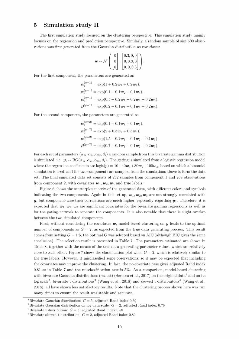
For the first component, the parameters are generated as
α(g=1)1 = exp(1 + 0.2w1 + 0.2w2),
α(g=1)2 = exp(0.1 + 0.1w2 + 0.1w3),
α(g=1)3 = exp(0.5 + 0.2w1 + 0.2w2 + 0.2w3),
β(g=1) = exp(0.2 + 0.1w1 + 0.1w2 + 0.2w3).
For the second component, the parameters are generated as
α(g=2)1 = exp(0.1 + 0.1w1 + 0.1w2),
α(g=2)2 = exp(2 + 0.3w2 + 0.3w3),
α(g=2)3 = exp(1.5 + 0.2w1 + 0.1w2 + 0.1w3),
β(g=2) = exp(0.7 + 0.1w1 + 0.1w2 + 0.2w3).
For each set of parameters (α1i, α2i, α3i, βi) a random sample from this bivariate gamma distribution
is simulated, i.e. yi ∼ BG(α1i, α2i, α3i, βi). The gating is simulated from a logistic regression model
where the regression coefficients are logit(p) = 10+40w1+30w2+100w3, based on which a binomial
simulation is used, and the two components are sampled from the simulations above to form the data
set. The final simulated data set consists of 232 samples from component 1 and 268 observations
from component 2, with covariates w1,w2,w3 and true labels.
Figure 6 shows the scatterplot matrix of the generated data, with different colors and symbols
indicating the two components. Again in this set-up, w1,w2,w3 are not strongly correlated with
y, but component-wise their correlations are much higher, especially regarding y2. Therefore, it is
expected that w1,w2,w3 are significant covariates for the bivariate gamma regressions as well as
for the gating network to separate the components. It is also notable that there is slight overlap
between the two simulated components.
First, without considering the covariates w, model-based clustering on y leads to the optimal
number of components as G = 2, as expected from the true data generating process. This result
comes from setting G = 1:5, the optimal G was selected based on AIC (although BIC gives the same
conclusion). The selection result is presented in Table 7. The parameters estimated are shown in
Table 8, together with the means of the true data-generating parameter values, which are relatively
close to each other. Figure 7 shows the classification plot when G = 2, which is relatively similar to
the true labels. However, it misclassified some observations, so it may be expected that including
the covariates may improve the clustering. In fact, the no-covariate case gives adjusted Rand index
0.81 as in Table 7 and the misclassification rate is 5%. As a comparison, model-based clustering
with bivariate Gaussian distributions (mclust) (Scrucca et al., 2017) on the original data1 and on its
log scale2, bivariate t distributions3 (Wang et al., 2018) and skewed t distribuitons4 (Wang et al.,
2018), all have shown less satisfactory results. Note that the clustering process shown here was run
many times to ensure the result was stable and accurate.
1Bivariate Gaussian distribution: G = 5, adjusted Rand index 0.392Bivariate Gaussian distribution on log data scale: G = 2, adjusted Rand index 0.763Bivariate t distribution: G = 3, adjusted Rand index 0.584Bivariate skewed t distribution: G = 2, adjusted Rand index 0.80
15

Y1
04
81
2−
1.5
0.0
1.0
2 4 6 8 10
0 2 4 6 8 10
Y2
w1
−1.5 −0.5 0.5 1.5
−1.5 −0.5 0.5 1.5
w2
24
68
−1
.50
.01
.5
−1.5 −0.5 0.5 1.5
−1
.50
.01
.0
w3
Figure 6: Scatter plot matrix of the simulated data set, colored by component membership: the
teal “�” is component 1 and the red “×” is component 2.
2 4 6 8 10
02
46
81
01
2
Y1
Y2
Figure 7: Classification when clustering y without covariates, with fitted distribution contours,
colored by membership: the teal “N” is component 1, the red “∗” is compoent 2. The optimal
model has G = 2.
16

Table 7: Model selection when setting G = 1:5. The selected optimal model has G = 2 (underlined).
log-likelihood AIC BIC Adjusted Rand Index
G=1 -2077.08 4162.17 4179.03 -
G=2 -1959.27 3936.53 3974.46 0.81
G=3 -1958.69 3945.38 4004.38 0.74
G=4 -1954.36 3946.71 4026.79 0.66
G=5 -1952.11 3952.21 4053.36 0.47
Table 8: Estimated parameters (θg) when G = 2 and no covariates included in the fitted model,
compared with the mean of the true data-generating parameters θg.
Component 1 Component 2
θg=1 θg=1 θg=2 θg=2
τg 0.50 0.49 0.50 0.51
α1g 2.74 2.49 1.11 2.14
α2g 1.10 0.81 7.48 9.37
α3g 1.65 1.53 4.48 3.51
βg 1.22 1.08 2.01 2.16
When incorporating the covariates w1,w2,w3 in the modeling process using a finite mixture of
bivariate gamma regressions, the model selection issue needs to be addressed again. Choices have
to be made for G, model type and covariates within each part of the expert and gating networks.
Stepwise forward selection is used, starting from a null model that is equivalent to fitting one
bivariate gamma distribution to y. The best selected models are presented in Table 9. These
models are designated as the best candidates selected by AIC. As expected, G = 2 is selected in all
cases, which coincides with the true simulation process. Although model 5 in Table 9 reflects the
true simulation process, the rest of the selected models are slightly better based on AIC, and are only
small modifications of model 5, which may be due to the small number of simulated observations.
This result shows that, although the data are generated using all covariates in all parts of α and
β, a parsimonious parameterisation effectively selects the most efficient parsimonious model. For
now, model 1 is taken as the best model for further investigation, although model 5 represents the
true simulation process and the prediction results are very similar among all models.
Table 9: The best five bivariate gamma MoE models selected according to AIC when covariates
are included in the models. Model 5 represents the true simulation process. Note that BIC gives
similar conclusion.
Model type G α1 expert α2 expert α3 expert β expert gating AIC BIC
1 VVC 2 w1 +w2 w2 +w3 w2 +w3 - w1 +w2 +w3 3323.35 3424.50
2 VVC 2 w1 +w2 w2 +w3 w1 +w2 +w3 - w1 +w2 +w3 3327.00 3436.58
3 VVV 2 w1 +w2 w2 +w3 w2 +w3 w1 +w3 w1 +w2 +w3 3329.45 3447.46
4 VVV 2 w1 +w2 w2 +w3 w1 +w2 +w3 w1 +w3 w1 +w2 +w3 3331.09 3457.52
5 VVV 2 w1 +w2 w2 +w3 w1 +w2 +w3 w1 +w2 +w3 w1 +w2 +w3 3334.23 3469.10
Figure 8(a) presents the clustering results for model 1, which suggests similar component struc-
ture to clustering without covariates. However, it is now able to separate the overlapping parts,
which gives an outcome very similar to the true class in Figure 6. In fact, the adjusted Rand
index is 0.98 with only two observations being misclassified. Hence, by using covariates in the
process of model-based clustering, it further improves the clustering result since extra information
17

is considered, which in turn leads to more insightful conclusions about the data and its dependence
structure. From a regression perspective, which is the main purpose of this method for predicting
claims given covariates while capturing different regression structures, fitted values of this model
are presented in Figure 8(b). Clearly this model is able to capture the two components with two
regression lines.
2 4 6 8 10
02
46
810
12
Y1
Y2
(a)
2 4 6 8 10
02
46
810
12
Y1
Y2
(b)
Figure 8: The best MoE model selected: (a) shows the classification plot of y, where the teal “N” is
component 1, the red “∗” is component 2; (b) shows the fitted values of the selected model, where
th true values are plotted in small black “�” and the predictions are plotted in red “�”.
Therefore, when covariates are incorporated the clustering fit is improved compared with the
case when no covariates are incorporated. From a regression perspective, using the proposed model
improved the (within-sample) fitted values. All of w1,w2,w3 entered all α-expert networks and
the gating network, while the parsimonious parameterisation captures the β parameter with no
covariates. The model regression parameters are given in Table 10. It shows that, in most cases,
the regression coefficients are close to the true simulation values. Figure 9 presents the boxplot of
the fitted values within each component. It shows that component 1 has mostly higher values of y1
than that of component 2, while y2 values in component 2 are greater than those in component 1,
which is consistent with Figure 8. Figure 9 also shows the calculated covariance between Y1 and Y2
18

Table 10: Estimated parameters of the selected MoE model: the top part shows the estimated gating
network regression coefficients (γ0), compared with the corresponding true values (γ0); the bottom
part shows the three sets of estimated regression coefficients for the α1, α2, α3 expert networks
(γ1g, γ1g, γ1g) and the estimated βg, compared with their true values γ1g,γ2g,γ3g and the mean of
βig (i.e. βg);
Gating network
intercept w1 w2 w3
γ0 10.00 40.00 30.00 100.00
γ0 12.55 59.31 43.82 141.34
Expert network
γ1g γ1g γ2g γ2g γ3g γ3g βg βg
Component g = 1
intercept 1.00 1.00 0.10 0.24 0.50 0.31
1.22 1.12w1 0.20 0.10 0.00 0.00 0.20 0.00
w2 0.20 0.05 0.10 -0.01 0.20 0.24
w3 0.00 0.00 0.10 0.68 0.20 -0.23
Component g = 2
intercept 0.10 0.30 2.00 2.18 1.50 1.49
2.01 2.32w1 0.10 0.65 0.00 0.00 0.20 0.00
w2 0.10 -0.28 0.30 0.21 0.10 0.16
w2 0.00 0.00 0.30 0.11 0.10 -0.03
from the fitted model, which indicates that the first component represents higher covariance than
the second component. In fact, the overall sample correlation between Y1 and Y2 is −0.01 in the
data. If not considering modeling the dependence structure, it may seem reasonable to model the
two risk perils independently. However, with the proposed approach the sample correlations within
components are 0.50 and 0.42 respectively. This shows that by modeling the dependence structure
directly the dependence captured is much stronger than it appears at the outset.
1 2
2.0
2.5
3.0
3.5
4.0
4.5
5.0
Component
Y1
1 2
23
45
67
8
Component
Y2
1 2
0.6
0.8
1.0
1.2
1.4
1.6
1.8
Component
Cov(Y
1,Y
2)
Figure 9: Boxplots of the fitted values within each component for the two responses Y1 and Y2, and
the fitted covariance between Y1, Y2 within each component.
19

For testing the predictive power of the model, a new test data set was generated with the same
method for N? = 200. The response variable y of the test set is presented in Figure 10(a), colored by
true component labels. The predicted cluster membership is shown in Figure 10(b), with adjusted
Rand index of 0.94 and only three observations misclassified. The predicted values of the selected
best model are shown in Figure 11(a). For comparison, standard GLMs using the same covariates
are also fitted using the simulated data respectively for y1 and y2, and the predicted values using
the test data are presented in Figure 11(b). It is clear that the univariate model did not capture
the structure within the data, and the best MoE model clearly identified the dependence structure
within different components.
2 4 6 8 10
02
46
810
12
Y1
Y2
(a)
2 4 6 8 10
02
46
810
12
Y1
Y2
(b)
Figure 10: Plot of the response variable y of the test data, generated using the same simulation
procedures as the training data: (a) the true cluster labels; (b) the predicted cluster labels using
the optimal model, where only three observations are misclassified.
To accurately assess the prediction improvement from using MoE models, the out-of-sample
predictions are assessed using various metrics, in comparison with the univariate GLM predictions.
It is important to evaluate the predictive performance of the predictive distributions generated,
relative to the respective observations with which the empirical distributions can be calculated,
such as predictive CDF versus empirical CDF. Key tools used to test different characteristics are:
20

2 4 6 8 10
02
46
810
12
Y1
Y2
(a)
2 4 6 8 10
02
46
810
12
Y1
Y2
(b)
Figure 11: Predicted values of y of the test data from (a) the optimal MoE model; (b) two inde-
pendent univariate GLMs. The true values are plotted in small black “�”, and the predictions are
plotted in red “�”.
proper scoring rule using the mean of continuous ranked probability score (CRPS) (Gschloßl &
Czado, 2007; Gneiting & Raftery, 2007); square root mean squared errors (rMSE) (Lehmann &
Casella, 2006); Gini index (Frees et al., 2014) and Wasserstein distance (Vallender, 1974). The
results are shown in Table 11. Particular interest lies in the predictions of the sum of Y1 and Y2,
since it represents the total risk, and the purpose of bivariate modeling is to better predict two
risks simultaneously while taking their dependence into account, especially in univariate modelling
the sum of models’ predictions would be taken as the total risk. It is also expected that predictions
within each marginal are improved. Table 11 shows that the MoE model clearly outperforms the
GLMs in all categories with the exception of Wasserstein distance for Y2 which is slightly worse.
6 Irish GI insurer data
A large motor insurance claims data set was obtained from an Irish general insurance company.
The data represent the insurer’s book of business in Ireland from January 2013 to June 2014, con-
taining 452,266 policies and their characteristics. In Ireland, motor insurance is required for all
motorists and is enforced by Irish law, with third party (TP) cover being the minimum requirement
21

Table 11: Comparisons between the MoE model and the GLM model for predictive performance
using a range of metrics. The underlined values represent the optimal results for each measure.
CRPS rMSE Gini Wasserstein
Sum of Y1, Y2MoE 1.83 2.71 0.55 1.15
GLM 1.86 2.95 0.54 1.26
Y1MoE 1.02 1.61 0.56 0.76
GLM 1.06 1.68 0.55 0.89
Y2MoE 1.48 1.64 0.62 0.80
GLM 1.48 2.10 0.61 0.74
(Houses of the Oireachtas, 1961). Across the portfolio, there are five distinct categories of claims:
accidental damage (AD), third party bodily injury (BI), third party property damage (PD), wind-
screen (WS) and theft (TF). This insurer provides two different types of coverage: third party, fire
and theft cover; and comprehensive cover (which includes all five categories). Typically, all five
categories are modeled independently, then the sum of predicted claims across the five categories
is taken as the total risk and the policy price is set based on this value. Because all five categories
and their pairwise dependencies were investigated, only comprehensive cover was selected.
Among the five categories covered per policy, AD and PD represent the highest correlation
(ρ(AD,PD) = 0.24) when excluding all policies for which no claims have been made on these two
categories. Hence only policies having made claims on both AD and PD were selected and their
depenence is chosen for investigation using the bivariate gamma distribution. Furthermore, in these
two categories there exist a few extremely large claims that are much greater than e20,000. These
observations have been deleted due to their extreme nature and it would be more appropriate to
utilise extreme value theory for modeling them. This leads to 2,074 policies being present in the
final data set. The logic of this work on severity is that, when a policyholder makes a claim only
in one category and not the other, the frequency models (either multivariate or univariate) will
account for this aspect. Bivariate severity models only investigate cases when claims are made on
both risks. It is worth noting that the correlation between AD and PD claims is not very strong,
although it represents the strongest correlation in the data. One may decide to use independent
modeling given this fact. However, it may also indicate that, since the data are very dispersed
(see Figure 12), there is underlying heterogeneity. By considering a clustering-based approach to
segregate the observations, the correlations between AD and PD within different components will
be much stronger. Bermudez (2009) concluded that, in the bivariate Poisson distribution case, even
when there are small correlations between claims, major differences can still occur in predictions
from a bivariate model compared with independent univariate models. It is shown that this same
outcome occurs for the bivariate gamma distribution case.
Table 12: Descriptions of the selected variables in the Irish GI data set. Note that “No claim
discount” represents the number of years with no claim.
Variables Categories
Vehicle fuel type Diesel; Petrol; Unknown
Vehicle transmission Automatic; Manual; Unknown
Annual mileage 0-5000; . . .; 45001-50000; 50001+
Number of registered drivers 1; 2; 3; 4; 5; 6; 7
No claim discount 0; 0.1; 0.2; 0.3; 0.4; 0.5; 0.6
No claim discount protection No; Yes; Unknown
Main driver license category B; C; D; F; I; N
22

0 2000 4000 6000 8000 10000 12000
050
0010
000
1500
020
000
AD
PD
(a)
0 2000 4000 6000 8000
020
0040
0060
0080
00
AD
PD
(b)
Figure 12: The plot of accidental damage (AD) and property damage (PD) claims of the Irish GI
data set: (a) shows all the claims; (b) shows the claims smaller than 8, 000 to give a clearer picture
of the clustering structure in the region where the majority of claims occur.
In the data set, there are about 100 variables presented. Due to data confidentiality issues,
not all significant predictors could be selected and used in this work. Seven key covariates are
used including policyholder’s information (e.g. licence category), insured car information (e.g. fuel
type, transmission) and policy information (e.g. no-claim discount). Table 12 shows the predictors
used and their categorical levels. It is expected that not all predictors will be significant, since it is
acknowledged that in general the severity model requires fewer predictors than the frequency model
(Coutts, 1984; Charpentier, 2014), and in a previous univariate modeling study using a similar data
set, it is also shown that not all the selected predictors provided here are significant (Hu et al.,
2018). Figure 12(a) shows the scatter plot of the AD and PD claim amounts. The claims from
23

the two risk perils are very dispersed, with only a few large claims in both risks. The scatters
are slightly more skewed towards PD, that is there are more policies having high PD and low AD
claim amounts and the number of large PD claim sizes is greater than the number of large AD
claims. There is no clear separation in the scatter plot, suggesting that different components (if
any) could be overlapped. There could also be clustering outliers and labelling noise present. The
vast majority of claims are heavily centred in the interval between 500 and 3, 000. A scatter plot
only focusing on the range AD ≤ 8, 000 and PD ≤ 8, 000 is presented in Figure 12(b) for better
clarity. In this plot, it is easier to see that, while there is a denser cluster in the interval between
500 and 3000, there are many claims close to both axes, indicating that many policies have slightly
high claim amounts in one peril but very low claim amounts in the other. The characteristics of
the data may explain why the overall correlation is low. By using the proposed method focusing
on dependence and segregating observations, it is expected that within homogeneous groups the
dependence will be much stronger, and therefore important to explicitly include in the model.
Table 13: Model selection when setting G = 1:7. The selected optimal model (based on AIC) gives
G = 4 (underlined). Note that BIC gives the same conclusion.
log-likelihood BIC AIC
G=1 -36392.69 72815.94 72793.39
G=2 -36310.17 72689.09 72638.36
G=3 -36292.07 72691.03 72612.11
G=4 -36245.94 72636.99 72529.89
G=5 -36244.47 72665.40 72530.11
G=6 -36238.72 72696.20 72532.72
G=7 -36236.37 72732.41 72540.75
0 2000 4000 6000 8000 10000 12000
050
0010
000
1500
020
000
AD
PD
Figure 13: Classification plot when clustering accidental damage (AD) and property damage (PD)
without covariates. The optimal number of components G = 4 using AIC. In the plot the green “�”
represents component 1, the yellow “∗” represents component 2, the blue “+” represents component
3 and the red “N” represents component 4.
24

0 2000 4000 6000 8000 10000 12000
050
0010
000
1500
020
000
AD
PD
Figure 14: Contour plot based on the fitted optimal number of components G = 4 when clustering
accidental damage (AD) and property damage (PD) without the covariates, corresponding to the
classification in Figure 13. In the plot the green, yellow, blue and red contours represent component
1, 2, 3 and 4 respectively. The plot shows that the four components are highly overlapping.
Starting with no covariates in the clustering process using a finite mixture of bivariate gamma
distributions, the method selects G = 4 using AIC, as shown in Table 13. Note that selection
based on BIC is also shown in Table 13, which gives the same conclusion. Figure 13 shows the
classification plot based on the optimal G = 4, while Figure 14 shows the corresponding contour
plot of the four fitted bivariate gamma distributions, based on the estimated parameters α,β
shown in Table 14. As mentioned earlier, there is a dense cluster of AD and PD claim sizes
in the interval between 500 and 3000, which has been recognized by the model (i.e. component
1). Other components include small claim sizes (AD < 1000 and PD < 4000) along the axes
(component 4), policies having made higher AD claim amounts than PD claims (component 3), and
policies having made PD claim amounts greater than or equal to AD claim amounts (component 2).
Figure 14 suggests heavy overlapping among the four components, which causes more uncertainty
when segregating the policyholders to amplify the dependencies. Within the four components, the
sample correlations now are (ρ(g=1) = 0.30, ρ(g=2) = 0.41, ρ(g=3) = 0.50, ρ(g=4) = −0.38), which
shows that the dependencies are much stronger once heterogeneity is considered, and the amplified
dependencies could be incorporated in simutaneous bivariate modeling.
Table 14: Estimated parameters when clustering accidental damage (AD) and property damge (PD)
without the covariates and G = 4 groups.
τg α1g α2g α3g βg
Component g=1 0.48 2.32 2.89 0.95 19.27*10−4
Component g=2 0.14 0.82 3.07 1.02 6.21*10−4
Component g=3 0.25 2.16 0.76 0.71 6.99*10−4
Component g=4 0.13 0.42 0.60 0.36 5.78*10−4
When including covariates in the proposed MoE model, model selection needs to be carefully
25

implemented using forward stepwise selection, and choices need to be made for G, model type
and covariates in each expert or gating networks (if any). It is worth noting that, since there are
7 covariates to select from together with all the model types in the model family, the potential
model space is huge. It may be reasonable to expect there are many models with similar predictive
power. The optimal model that has been selected based on AIC is presented in Table 15. The
selected optimal model has model type “VVV”, G=4 and AIC= 72, 583.97. G is consistent with the
result with no covariates as before. Annual mileage and no-claim discount (NCD) are not selected
in the final model, while the rest of covariates enter either one or more of the expert or gating
networks. Noticeably the gating network and the β-expert have the most covariates, which makes
sense because: (1) it helps to allocate observations into the correct components while within each
component the dependence may be simpler to model given the correct allocation; (2) the claim
amount range within the data set (from close to 0 to 20, 000) is large, which may require more
covariates to model the rate parameter β to separate the smaller and larger claims.
Table 15: Selected covariates in each gating and expert network of the optimal model, which has
G = 4 and model type “VVV”.
α1 expert α2 expert α3 expert β expert gating
Vehicle fuel type√ √ √ √
Vehicle transmission√ √ √
Annual mileage
Number of registered drivers√
No claim discount (NCD)
No claim discount protection√ √ √ √
Main driver license category√ √
0 2000 4000 6000 8000 10000 12000
05
00
01
00
00
15
00
02
00
00
AD
PD
Figure 15: Classification of accidental damage (AD) and property damage (PD) of the selected
VVV model with G = 4, where the green “�” represents component 1, the yellow “∗” represents
component 2, the blue “+” represents component 3 and the red “N” represents component 4.
The classification plot based on the optimal model is shown in Figure 15. The general pattern is
26

similar to that in Figure 13, where component 1 captures the dense claim size cloud of AD and PD
in the interval 500−4000, component 2 captures large claim amounts particularly when PD > AD
, component 3 captures AD claims greater than PD and component 4 captures small claims of PD
greater than AD, which consists of the fewest policies. It is useful and important to see that the
dependence structures captured here are consistent with the case where no covariates are included,
in Figure 13. However, this result makes more sense and has the following differences compared
with Figure 13: (1) there are more policies having higher AD and very low PD claims (i.e. more
scatters along the AD-axis from 0), this feature is now better captured by component 3; (2) there
are some policies having higher PD and very low AD claims, but when PD amounts are larger than
5000, they also tend to have slightly higher AD amounts, hence component 4 mostly captures a
small proportion of policies having relatively small PD amounts and very small (close to 0) AD
amounts; (3) component 2 not only captures large PD claims greater than AD, but also overall
large claim amounts for both AD and PD; but because of the scarcity of very large claims overall,
alternatively it can be interpreted as the large claims noise component. Note that because this
classification is a result of incorporating covariates in regressions, it makes more sense to see that
not only there are clear overlaps among all components, but also the component boundaries are
more blurred. There are a few observations (for example, a few policies labelled red N in component
4 in Figure 15) set apart from their corresponding components clearly, aside from the covariates’
influence this could also potentially be due to outliers or labelling noise in the data.
Based on this classification the sample correlations for the four components are (ρ(g=1) =
0.33, ρ(g=2) = 0.05, ρ(g=3) = 0.41, ρ(g=4) = 0.72) respectively. In most cases the correlation within
component is stronger than the overall correlation (ρ = 0.24). Component 2 has very low sample
correlations, which could be due to the fact that it captures mostly overall large claims, as an
overall “noise” component. It again shows that by segregating the data based on the dependence
structure directly, within component the dependencies are indeed much stronger than it may first
appear.
When different (combinations of) covariates enter different expert networks, it might make
model interpretation more difficult. In the selected model, vehicle transmission, number of regis-
tered drivers, NCD protection and main driver licence category enter the gating networks, which
explicitly control which component the policy belongs to, although covariates in each expert also
implicitly control the choice of components (Bermudez & Karlis (2012)). Each of the expert net-
works has different covariates. Covariance is mainly determined by α3 (and β). It is interesting to
see only vehicle fuel type and NCD protection enter this α3 network, indicating vehicle fuel types
and NCD protection affect much of the dependence between AD and PD. The optimal model is
chosen based on AIC. While it penalises extra paramters less than other metrics such as BIC, it is
still surprising to see that in most of the expert networks not many covariates are involved. For
the proposed MoE model family, since very likely G ≥ 2, adding a covariate into the model means
G times more parameters in the covariate are added. This largely leads to it prefering a simpler
model set up.
Figure 16 shows the final fitted values of the model across all components. The fitted values
cover a wide range of values and capture the very small and large claim amounts. However, they
did not capture the very large claims, such as when policies have very large AD claim amounts
greater than 6000 or large PD amounts greater 10, 000. One potential reason is the limited number
of covariates used or available to use. In each of the expert networks only two covariates are used,
which are categorical variables with only a limited number of levels. Hence the model might not be
able to capture a lot of variation within each component. More importantly, it could be because
the data are long tailed, with only a few claims having large AD or PD amounts, especially when
AD and PD are greater than 8000.
Figure 17 presents the boxplot of the fitted values within each component before mixing for a
clearer picture of comparisons among components. It shows that components 2 and 3 have mostly
higher values of AD, while component 2 also has mostly high risk on PD. These are consistent
27

with Figure 15 in that component 2 captures mostly large AD and PD claims. Component 1 has
medium risk on both AD and PD, while component 4 has very small AD risk but slightly higher
PD risk. While Figure 17 shows large variations of predictions among different components, it is
noted that, in the gating network, the fitted mixing probabilities mostly range between 40% and
70% to classify observations to each component. Hence, after mixing, the overall predictions are
pulled away from the within-component predictions. This is mainly due to the overlapping nature
of the components, and possibly lack of additional covariates in the data. If the clusters are more
separated, or extra information (covariates) is included in the gating network, which may lead to
the mixing probabilities being closer to 0 or 1 (i.e. the components are better separated by the
MoE model), then predictions could be expected to perform even better.
0 2000 4000 6000 8000 10000 12000
050
0010
000
1500
020
000
AD
PD
Figure 16: Fitted values of accidental damage (AD) and property damage (PD) using the selected
VVV model with G = 4. The given observations are plotted using a small black “�”, while the
predictions are plotted using a red “�”
1 2 3 4
020
0040
0060
0080
00
Component
AD
(a)
1 2 3 4
010
0020
0030
0040
0050
0060
0070
00
Component
PD
(b)
Figure 17: Boxplots of the fitted values within each component of the optimal model for the two
claim types before mixing: (a) shows accidental damage (AD); (b) shows property damage (PD).
28

0 2000 4000 6000 8000 10000
050
0010
000
1500
0
AD
PD
(a)
0 2000 4000 6000 8000 10000
050
0010
000
1500
0
AD
PD
(b)
Figure 18: Predicted values of accidental damge (AD) and property damage (PD) for the test data
set: (a) is the result of the selected optimal MoE model; (b) is the result of the standard univariate
GLMs. The true values are plotted in small black “�”, while the predictions are plotted in red “�”.
For predictions, the data set is split into a training set (N=1874) and a test set (N=200).
Figure 18(a) shows the predicted values of AD and PD on the test set, while the model is trained
using the training set with the previously selected optimal model. Similarly as in the simulation
studies, standard univariate GLMs are fitted for AD and PD respectively based on the training
set and predicted on the test set, using the same set of selected covariates. The predictions are
shown in Figure 18(b). By comparing the two figures, it is clear that the MoE model predictions
outperform the GLM predictions, with the MoE predictions spanning a wide range and predicting
very small claim amounts and large claim amounts for AD, which can be interpreted as the different
dependence structures in the data set being captured. To assess the prediction improvements,
various metrics are used, as in Section 4 and 5 for the simulation studies. They evaluate the
predictive distributions of the model compared with the empirical distributions calculated using
the observations. The results are shown in Table 16. The primary focus for this table is the sum of
AD and PD, because it represents the overall total risk of policyholders, and traditionally different
perils would be modeled independently, and their sum taken as the total risk. The purpose of
the MoE method is that total claim amounts be better predicted when taking the dependence
structure into consideration. The MoE model outperforms the GLM in all categories in this case,
and the improvement is prominent. It is also expected that, by modeling two risks simultaneously
and considering their dependency, the understanding and predictions of each marginal risk are
29

also improved. For each margin, Table 16 shows strong improvement, except when considering
PD, where rMSE and Gini index are slightly worse, while the rest of the metrics show a clear
improvement. It is consistent with Figure 18, since in the plot the range of predicted PD claims is
similar for both models. This could possibly be due to the fact that PD claims may be affected by
other factors not available in the selected data. Overall it shows that by taking the covariance into
account when modeling two risks simultaneously via the bivariate gamma distribution, and taking
the heterogeneity into account for enhanced covariance, it leads to better model predictions and
improved understanding of the data structure.
Table 16: Comparisons between the MoE model and the GLM model for predictive performance
regarding accidental damage (AD) and property damage (PD) using the mean of continuous ranked
probability score (CRPS), square root mean squared errors (rMSE), Gini index and Wasserstein
distance, as discussed before. The underlined values represent the optimal resutls for each measure.
CRPS rMSE Gini Wasserstein
Sum of AD and PDMoE 2421.38 3966.90 0.54 2159.26
GLM 2466.63 3998.07 0.52 2216.94
ADMoE 1203.19 1854.32 0.55 1002.13
GLM 1226.90 1867.72 0.54 1062.82
PDMoE 1559.13 2786.93 0.52 1431.44
GLM 1600.67 2786.24 0.53 1481.59
7 Conclusion
This work investigated the application of bivariate gamma distributions in the framework of
mixture of experts models for insurance claims modeling. More specifically, a finite mixture of
bivariate gamma regressions within a GLM framework is investigated, focusing on predicting future
claims. In doing so, not only is covariance taken into account in regressions for simultaneously
modeling of two risks, but different claim patterns could be identified with different dependence
structures targeting the heterogeneity issue. This leads to amplified within-component dependencies
even when the overall dependence of all data is weak. The bivariate gamma distribution is a natural
extension of the univariate gamma GLM when independence between different risk perils is revoked.
It has been shown that claim predictions could be improved for both simulation data sets and the
real Irish GI insurer data by using the proposed method. This is done by assessing the sum of the
two margins or assessing individual margins independently, since traditionally in GI claim modeling
each category is modeled independently and the sum of all categories is taken as the total risk.
This method could be viewed from two perspectives - claim clustering and claim prediction
by regression - both taking the dependence structure into consideration. By viewing it from a
clustering perspective, given the data are bivariate gamma distributed (which is typically the case
for GI claim severity modeling), model-based clustering with the bivariate gamma distributions
can segregate the policyholders with different claim-making behaviours into different groups, hence
the dependence structure is enhanced and better captured. Furthermore, by including covariates
in the clustering process, the result is further improved. By viewing it from a regression prediction
perspective, the model is essentially equivalent to a mixture of regressions by fitting multiple
regressions that model different patterns in the data while combining the different regression lines
via a logistic regression at the same time.
Within the bivariate gamma MoE model family, various parameterisations have been proposed
to facilitate parsimonious model selection, which allows covariates to enter all or some of the
30

expert networks and the gating network. It is also noted that, because covariates entering into
different networks may be different, it can lead to interpretability difficulties. The selection of
covariates should also be done carefully, as the effect of the number of covariates on increasing
the potential model space is huge, and it will lead to more computational complexity in practice.
Furthermore, with G increasing, adding one covariates will lead to G times more parameters in the
model, hence stepwise selection will often prefer a simpler model. Although the simplest option
could be that all covariates are included in all parts, this could lead to model parsimony issues.
We note that variable selection cannot be done by hypothesis testing within each GLM structure
involved, hence model selection should be carefully implemented to facilitate easier and better
model interpretation. If model parsinony is not of primary concern, another possible solution is to
utilise logical or expert intuition rather than strictly following a stepwise model selection approach.
For example, in Bermudez & Karlis (2012) G is logically chosen based on the characteristics of
their insurance claim frequency count data.
One issue with this bivariate gamma distribution is the computational complexity of its den-
sity function, which has prohibited its widespread use in the past. When extending to higher
dimensional cases as in Section 2, the computation becomes even more complex because it requires
multiple numerical integrations depending on specification of the dependence structures. Further
exploration on the higher dimensional cases could constitute future work, in which case the model
selection will also involve selecting different dependence structure assumptions. Furthermore, since
the sufficient statistics of the gamma distribution are X and logX, by implementing the maximum
likelihood approach using the EM algorithm, even more computational complexity is introduced,
which involves numerical integrations and numerical optimisations in both E and M-steps. When
the tolerance in the EM algorithm is too small, the complexity of numerical computations might
sometimes not be able to guarantee the monotonicity of the log-likelihood towards the very end of
the algorithm. It creates potential obstacles in the implementation of this model including compu-
tational stability, accuracy and speed. Parameter tuning should be carefully implemented to ensure
the numerical calculations always achieve the best possible results.
In the Irish GI insurer section, the heavily overlapped components cause much of the uncertainty
on cluster membership, and there are scarce numbers of very large claims with associated claims
data, both affecting the final predictions of the model. In this work an Expectation/Conditional
Maximization algorithm (ECM) (Meng & Rubin, 1993) is used for the maximum likelihood ap-
proach. Other variations of the EM algorithm could be adapted such as Classification EM (CEM)
(Celeux & Govaert, 1992), which may give less fuzzy clustering results and faster convergence. Al-
ternatively, if only regarding the proposed method as a clustering approach (i.e. to segregate data
for amplified dependence structure), after clustering, separate regressions (either bivariate gamma
regressions or univariate GLMs) could be fitted within each component independently to improve
the model predictions. In this case, for better clustering results, potentially one can either treat
the extreme large claims as outliers and use trimming techniques from the clustering literature, or
add an extra component capturing random noise. This could also consitute future work.
If stepwise selection is used, with the number of covariates and G increasing, the potential
model space can be huge. It may be reasonable to expect that there are many models with similar
goodness-of-fit and predictive power. This could suggest a model averaging approach as future
work, similar to the works of Wei & McNicholas (2015), Russell et al. (2015), Hu et al. (2018),
where either clustering results, regression predictions or categorical variables’ construction can be
merged.
Acknowledgements
This work was supported by the Science Foundation Ireland funded Insight Research Centre
(SFI/12/RC/2289).
31

References
Aitken, AC (1927), ‘On Bernoulli’s numerical solution of algebraic equations,’ Proceedings of the
Royal Society of Edinburgh, 46, pp. 289–305.
Akaike, H (1974), ‘A new look at the statistical model identification,’ IEEE Transactions on Au-
tomatic Control, 19(6), pp. 716–723.
Asimit, AV, Furman, E & Vernic, R (2010), ‘On a multivariate Pareto distribution,’ Insurance:
Mathematics and Economics, 46(2), pp. 308–316.
Balakrishna, N & Lai, CD (2009), ‘Bivariate gamma and related distributions,’ in Lai, CD &
Balakrishnan, N (eds.), Continuous bivariate distributions, Springer, New York, 2 edn.
Bermudez, L (2009), ‘A priori ratemaking using bivariate Poisson regression models,’ Insurance:
Mathematics and Economics, 44(1), pp. 135–141.
Bermudez, L & Karlis, D (2012), ‘A finite mixture of bivariate Poisson regression models with
an application to insurance ratemaking,’ Computational Statistics & Data Analysis, 56(12), pp.
3988–3999.
Biernacki, C, Celeux, G & Govaert, G (2000), ‘Assessing a mixture model for clustering with the
integrated completed likelihood,’ IEEE Transactions on Pattern Analysis and Machine Intelli-
gence, 22(7), pp. 719–725.
Bishop, CM (2006), Pattern Recognition and Machine Learning, Springer-Verlag, New York.
Bohning, D, Dietz, E, Schaub, R, Schlattmann, P & Lindsay, BG (1994), ‘The distribution of the
likelihood ratio for mixtures of densities from the one-parameter exponential family,’ Annals of
the Institute of Statistical Mathematics, 46(2), pp. 373–388.
Celeux, G & Govaert, G (1992), ‘A classification EM algorithm for clustering and two stochastic
versions,’ Computational Statistics & Data Analysis, 14(3), pp. 315–332.
Charpentier, A (2014), Computational actuarial science with R, CRC Press, Boca Raton.
Cheriyan, K (1941), ‘A bivariate correlated gamma-type distribution function,’ Journal of the
Indian Mathematical Society, 5, pp. 133–144.
Chiragiev, A & Landsman, Z (2007), ‘Multivariate pareto portfolios: TCE-based capital allocation
and divided differences,’ Scandinavian Actuarial Journal, 2007(4), pp. 261–280.
Coutts, SM (1984), ‘Motor insurance rating, an actuarial approach,’ Journal of the Institute of
Actuaries (1886-1994), 111(1), pp. 87–148.
Dempster, AP, Laird, NM & Rubin, DB (1977), ‘Maximum likelihood from incomplete data via
the EM algorithm,’ Journal of the Royal Statistical Society. Series B (Methodological), 39, pp.
1–38.
Everitt, B, Landau, S, Leese, M & Stahl, D (2011), Cluster Analysis, Wiley Series in Probability
and Statistics, Wiley, West Sussex, 5 edn.
Frees, EW, Lee, G & Yang, L (2016), ‘Multivariate frequency-severity regression models in insur-
ance,’ Risks, 4(1), 4.
Frees, EW & Valdez, EA (1998), ‘Understanding relationships using copulas,’ North American
Actuarial Journal, 2(1), pp. 1–25.
32

Frees, EWJ, Meyers, G & Cummings, AD (2014), ‘Insurance ratemaking and a Gini index,’ Journal
of Risk and Insurance, 81(2), pp. 335–366.
Furman, E (2008), ‘On a multivariate gamma distribution,’ Statistics & Probability Letters, 78(15),
pp. 2353–2360.
Furman, E & Landsman, Z (2005), ‘Risk capital decomposition for a multivariate dependent
Gamma portfolio,’ Insurance: Mathematics and Economics, 37(3), pp. 635–649.
Furman, E & Landsman, Z (2008), ‘Economic capital allocations for non-negative portfolios of
dependent risks,’ ASTIN Bulletin, 38(2), pp. 601–619.
Furman, E & Landsman, Z (2010), ‘Multivariate Tweedie distributions and some related capital-
at-risk analyses,’ Insurance: Mathematics and Economics, 46(2), pp. 351–361.
Gneiting, T & Raftery, AE (2007), ‘Strictly proper scoring rules, prediction, and estimation,’
Journal of the American Statistical Association, 102(477), pp. 359–378.
Gormley, IC & Murphy, TB (2011), ‘Mixture of experts modelling with social science applications,’
in Mengersen, K, Robert, C & Titterington, M (eds.), Mixture: estimation and applications,
Wiley, West Sussex.
Grazian, C & Liseo, B (2015), ‘Approximate Bayesian computation for copula estimation,’ Statis-
tica, 75(1), pp. 111–127.
Grun, B & Leisch, F (2008), ‘Finite mixtures of generalized linear regression models,’ in Shalabh
& Heumann, C (eds.), Recent advances in linear models and related areas: essays in honour of
Helge Toutenburg, Physica-Verlag, Heidelberg.
Gschloßl, S & Czado, C (2007), ‘Spatial modelling of claim frequency and claim size in non-life
insurance,’ Scandinavian Actuarial Journal, 2007(3), pp. 202–225.
Houses of the Oireachtas (1961), ‘Road traffic act,’ http://www.irishstatutebook.ie/eli/1961/
act/24/enacted/en/print, assessed 26 Jun. 2017.
Hu, S, O’Hagan, A & Murphy, TB (2018), ‘Motor insurance claim modelling with factor collapsing
and Bayesian model averaging,’ Stat, 7(1), p. e180.
Huang, GH & Bandeen-Roche, K (2004), ‘Building an identifiable latent class model with covariate
effects on underlying and measured variables,’ Psychometrika, 69(1), pp. 5–32.
Jacobs, RA, Jordan, MI, Nowlan, SJ & Hinton, GE (1991), ‘Adaptive mixtures of local experts,’
Neural computation, 3, pp. 79–87.
Jensen, DR (1969), ‘An inequality for a class of bivariate Chi-square distributions,’ Journal of the
American Statistical Association, 64, pp. 333–336.
Joe, H (1997), Multivariate models and multivariate dependence concepts, Chapman and Hall/CRC,
New York.
Karlis, D & Meligkotsidou, L (2005), ‘Multivariate Poisson regression with covariance structure,’
Statistics and Computing, 15(4), pp. 255–265.
Karlis, D & Meligkotsidou, L (2007), ‘Finite mixtures of multivariate Poisson distributions with
application,’ Journal of Statistical Planning and Inference, 137(6), pp. 1942–1960.
Karlis, D & Ntzoufras, I (2003), ‘Analysis of sports data by using bivariate Poisson models,’ Journal
of the Royal Statistical Society: Series D (The Statistician), 52(3), pp. 381–393.
33

Kim, D & Lindsay, BG (2015), ‘Empirical identifiability in finite mixture models,’ Annals of the
Institute of Statistical Mathematics, 67(4), pp. 745–772.
Kotz, S, Balakrishnan, N & Johnson, NL (2000), ‘Multivariate Gamma distributions,’ in Continuous
Multivariate Distributions, Volume 1: Models and Applications, John Wiley & Sons, Inc., New
York.
Lee, SCK & Lin, XS (2012), ‘Modeling dependent risks with multivariate Erlang mixtures,’ ASTIN
Bulletin, 42(1), pp. 153–180.
Lehmann, E & Casella, G (2006), Theory of point estimation, Springer New York.
Mathai, AM & Moschopoulos, PG (1991), ‘On a multivariate gamma,’ Journal of Multivariate
Analysis, 39(1), pp. 135–153.
Meng, XL & Rubin, DB (1993), ‘Maximum likelihood estimation via the ECM algorithm: A general
framework,’ Biometrika, 80(2), pp. 267–278.
Mikosch, T (2006), ‘Copulas: tales and facts,’ Extremes, 9(1), pp. 3–20.
Murhpy, K & Murphy, TB (2015), ‘Gaussian parsimonious clustering models with covariates,’ arXiv
preprint arXiv:1506.09035.
Nelder, JA & Wedderburn, RWM (1972), ‘Generalized linear models,’ Journal of the Royal Statis-
tical Society. Series A (General), 135(3), pp. 370–384.
Panjer, HH (2002), ‘Measurement of risk, solvency requirements and allocation of capital within
financial conglomerates,’ Research Report, Institute of Insurance and Pension Research, Univer-
sity of Waterloo, pp. 01–15.
Ramabhadran, V (1951), ‘A multivariate Gamma-type distribution,’ Sankhya, 11, pp. 45–46.
Rothenberg, TJ (1971), ‘Identification in parametric models,’ Econometrica, 39(3), pp. 577–591.
Russell, N, Murphy, TB & Raftery, AE (2015), ‘Bayesian model averaging in model-based clustering
and density estimation,’ arXiv preprint arXiv:1506.09035.
Schwarz, G (1978), ‘Estimating the dimension of a model,’ The Annals of Statistics, 6(2), pp.
461–464.
Scrucca, L, Fop, M, Murphy, TB & Raftery, AE (2017), ‘mclust 5: clustering, classification and
density estimation using Gaussian finite mixture models,’ The R Journal, 8(1), pp. 205–233.
Tsionas, EG (2004), ‘Bayesian inference for multivariate Gamma distributions,’ Statistics and Com-
puting, 14(3), pp. 223–233.
Vaidyanathan, V & Lakshmi, RV (2015), ‘Parameter estimation in multivariate Gamma distribu-
tion,’ Statistics, Optimization & Information Computing, 3(2), pp. 147–159.
Vallender, S (1974), ‘Calculation of the Wasserstein distance between probability distributions on
the line,’ Theory of Probability & Its Applications, 18(4), pp. 784–786.
Vrieze, SI (2012), ‘Model selection and psychological theory: a discussion of the differences be-
tween the Akaike information criterion (AIC) and the Bayesian information criterion (BIC),’
Psychological Methods, 17(2), pp. 228–243.
Wang, K, Ng, A & McLachlan., G (2018), EMMIXskew: The EM Algorithm and Skew Mixture
Distribution, R package version 1.0.3.
34

Wang, Z & Zhou, XH (2014), ‘Nonparametric identifiability of finite mixture models with covariates
for estimating error rate without a gold standard,’ UW Biostatistics Working Paper Series,
1(403).
Wei, Y & McNicholas, PD (2015), ‘Mixture model averaging for clustering,’ Advances in Data
Analysis and Classification, 9(2), pp. 197–217.
Willmot, GE & Woo, JK (2015), ‘On some properties of a class of multivariate Erlang mixtures
with insurance applications,’ ASTIN Bulletin, 45(1), pp. 151–173.
Yang, Y (2005), ‘Can the strengths of AIC and BIC be shared? A conflict between model indenti-
fication and regression estimation,’ Biometrika, 92(4), pp. 937–950.
Yue, S, Ouarda, T & Bobee, B (2001), ‘A review of bivariate Gamma distributions for hydrological
application,’ Journal of Hydrology, 246(1), pp. 1–18.
35

Appendix
A Proof of E(Y ), V ar(Y ) and Cov(Y ).
The bivariate gamma distribution can be defined as Y = AX, where X = (X1, X2, X3)>,
A =
[1 0 1
0 1 1
].
Then the conditional expectation and variance-covariance matrix of Y are
E[Y |α, β] = E[AX] = Aθ,
V ar[Y |α, β] = AΣA>,
where θ = (α1/β, α2/β, α3/β)>,Σ = diag(α1/β2, α2/β
2, α3/β2),α = (α1, α2, α3)>. When Y fol-
lows a finite mixture of bivariate gamma distributions, the unconditional expectation of Y is
E[Y ] = E[E[Y |α,β]] = AE[θ] = A
E[α1/β]
E[α2/β]
E[α3/β]
= A
∑g τgα1g/βg∑g τgα2g/βg∑g τgα3g/βg
=
[∑g τg
α1g+α3g
βg∑g τg
α2g+α3g
βg
],
where α = (α1,α2,α3)>, α1 = (α1,g=1, . . . , α1,g=G)>, β = (βg=1, . . . , βg=G)>. To calculate the
unconditional variance of Y , first the second moment of Y conditional on all α,β is
E[Y Y >|α,β] = V ar[Y |α,β] + E[Y |α,β][E[Y |α,β]]>
= AΣA> +Aθ[Aθ]>
= AB(α,β)A>,
where
B(α,β) = Σ + θθ> =
α2
1
β2 + α1
β2α1α2
β2α1α3
β2
α1α2
β2
α22
β2 + α2
β2α2α3
β2
α1α3
β2α2α3
β2
α23
β2 + α3
β2
.This shows that the conditional second moment is polynomial with respect to α and β. Hence
E[Y Y >] = E[E[Y Y >|α,β]] by the law of total expectation. The element-wise expectation of
the matrix B(α,β) is denoted as E[B], then E[Y Y >] = AE[B]A>, and the variance-covariance
matrix of Y is
V ar(Y ) = E[Y Y >]− E[Y ][E[Y ]]>
= AE[B]A> −AE[θ][AE[θ]]>
= A[E[B]− E[θ]E[θ]>
]A>
= AD(α,β)A>,
where
D(α,β) =
V ar(α1
β ) + E(α1
β ) Cov(α1
β ,α2
β ) Cov(α1
β ,α3
β )
Cov(α1
β ,α2
β ) V ar(α2
β ) + E(α2
β ) Cov(α2
β ,α3
β )
Cov(α1
β ,α3
β ) Cov(α2
β ,α3
β ) V ar(α3
β ) + E(α3
β )
.Hence
V ar(Y1) = V ar(α1
β) + E(
α1
β) + V ar(
α3
β) + E(
α3
β) + 2Cov(
α1
β,α3
β) ,
V ar(Y2) = V ar(α2
β) + E(
α2
β) + V ar(
α3
β) + E(
α3
β) + 2Cov(
α2
β,α3
β) ,
Cov(Y1,Y2) = Cov(α1
β,α2
β) + Cov(
α1
β,α3
β) + Cov(
α2
β,α3
β) + V ar(
α3
β) + E(
α3
β) .
36

B Distribution estimation
This section introduces distribution estimation for the bivariate gamma distribution using the
EM algorithm for likelihood maximisation. Defined as in Equation (1), the distribution has one
latent variable X3, while X1, X2, X3 are independent. Therefore, the complete data log-likelihood
is
`c =
N∑i=1
log p(x3, y1i, y2i; θ),
and the conditional expectation of the log-likelihood in the E-step at the tth iteration is
Q(θ(t+1)|θ(t)) = E
[N∑i=1
log p(x3, y1i, y2i; θ(t+1)) | y1, y2, θ(t)
].
The sufficient statistics are X3, log(X3), log(y1−X3), log(y2−X3). The EM algorithm is as follows:
E-step
x(t+1)3i = E(X3i|y1i, y2i; θ(t)) =
α(t)3
β(t)p(y1i, y2i; α
(t)1 , α
(t)2 , α
(t)3 + 1, β(t))
p(y1i, y2i; α(t)1 , α
(t)2 , α
(t)3 , β(t))
,
x(t+1)1i = E(X1i|y1i, y2i; θ(t)) = E(y1i −X3i|y1i, y2i; θ(t)) = y1 − x(t+1)
3i ,
x(t+1)2i = E(X2i|y1i, y2i; θ(t)) = E(y2i −X3i|y1i, y2i; θ(t)) = y2 − x(t+1)
3i ,
log x(t+1)
3i = E(logX3i|y1i, y2i; θ(t)) =
∫min(y1i,y2i)
0log x3ip(x3i, y1i, y2i; θ
(t))dx3
p(y1i, y2i; θ(t)),
log x(t+1)
1i = E(log(y1i −X3i)|y1i, y2i; θ(t)) =
∫min(y1i,y2i)
0log(y1i − x3i)p(x3i, y1i, y2i; θ(t))dx3
p(y1i, y2i; θ(t)),
log x(t+1)
2i = E(log(y2i −X3i)|y1i, y2i; θ(t)) =
∫min(y1i,y2i)
0log(y2i − x3i)p(x3i, y1i, y2i; θ(t))dx3
p(y1i, y2i; θ(t)).
M-step
For α(t+1)1 , α
(t+1)2 , α
(t+1)3 , numerically solve the following equations respectively:
N log β(t) −N Γ′(α1)
Γ(α1)+
N∑1=i
log x(t+1)
1i = 0,
N log β(t) −N Γ′(α2)
Γ(α2)+
N∑1=i
log x(t+1)
2i = 0,
N log β(t) −N Γ′(α3)
Γ(α3)+
N∑1=i
log x(t+1)
3i = 0.
β(t+1) =N(α
(t+1)1 + α
(t+1)2 + α
(t+1)3 )∑N
i=1(x(t+1)1i + x
(t+1)2i + x
(t+1)3i )
.
37

C EM algorithms for all model types within bivariate gamma
MoE model family
For the EM algorithm for all model types within the bivariate gamma MoE model family as
shown in Table 2, the E-step is always the same, except for the parameterisations of α1, α2, α3 and
β. Note that the gating network derivation is the same for all model types as shown in Section 3
of the main text, hence is not shown here. The “II” model type is estimating one bivarite gamma
distribution parameters, which has been shown in Appendix B. The “∗CC”, “∗CI” “∗IC” types can
be easily derived similarly based on this section and Appendix B. At the tth iteration, the E-step
and M-step are:
E-step
z(t+1)ig = E(zig|y1i, y2i, θ(t)g (wi))
x(t+1)3ig = E(X3ig|y1i, y2i; θ(t)g (wi))
x(t+1)1ig = E(y1i −X3ig|y1i, y2i; θ(t)g (wi)) = y1i − x(t+1)
3ig
x(t+1)2ig = E(y2i −X3ig|y1i, y2i; θ(t)g (wi)) = y2i − x(t+1)
3ig
log x(t+1)
3ig = E(logX3ig|y1i, y2i; θ(t)g (wi))
log x(t+1)
1ig = E(log(y1i −X3i)|y1i, y2i; θ(t)g (wi))
log x(t+1)
2ig = E(log(y2i −X3i)|y1i, y2i; θ(t)g (wi))
M-step
• “∗VC” model type:
Update γ(t+1)kg (k = 1, 2, 3):
γ(t+1)kg = arg max
γkg
(N∑i=1
z(t+1)ig exp(γ>kgwki) log β(t)
g −N∑i=1
z(t+1)ig log Γ(exp(γ>kgwki))
+
N∑i=1
z(t+1)ig exp(γ>kgwki)log x
(t+1)
kig
).
Update β(t+1)g :
β(t+1)g =
∑Ni=1 z
(t+1)ig
(α(t+1)1ig + α
(t+1)2ig + α
(t+1)3ig
)∑Ni=1 z
(t+1)ig
(x(t+1)1ig + x
(t+1)2ig + x
(t+1)3ig
) .• “∗CV” model type:
Update α(t+1)kg (k = 1, 2, 3) by solving
N∑i=1
z(t+1)ig log β
(t)ig −
N∑i=1
z(t+1)ig
Γ′(αkg)
Γ(αkg)+
N∑i=1
z(t+1)ig log x
(t+1)
kig = 0.
Update γ(t+1)4g :
γ(t+1)4g = arg max
γ4g
((α
(t+1)1g + α
(t+1)2g + α
(t+1)3g )
N∑i=1
z(t+1)ig (γ>4gw4i)
−N∑i=1
z(t+1)ig exp(γ>4gw4i)(x
(t+1)1ig + x
(t+1)2ig + x
(t+1)3ig )
).
38

• “∗VV” model type:
Update γ(t+1)kg (for k = 1, 2, 3):
γ(t+1)kg = arg max
γkg
(N∑i=1
z(t+1)ig exp(γ>kgwki) log β
(t)ig −
N∑i=1
z(t+1)ig log Γ(exp(γ>kgwki))
+
N∑i=1
z(t+1)ig exp(γ>kgwki)log x
(t+1)
kig
).
Update γ(t+1)4g :
γ(t+1)4g = arg max
γ4g
(N∑i=1
z(t+1)ig (α
(t+1)1ig + α
(t+1)2ig + α
(t+1)3ig )(γ>4gw4i)
−N∑i=1
z(t+1)ig exp(γ>4gw4i)(x
(t+1)1ig + x
(t+1)2ig + x
(t+1)3ig )
).
• “∗VI” model type:
Update γ(t+1)kg (k = 1, 2, 3):
γ(t+1)kg = arg max
γkg
(N∑i=1
z(t+1)ig exp(γ>kgwki) log β(t) −
N∑i=1
z(t+1)ig log Γ(exp(γ>kgwki))
+
N∑i=1
z(t+1)ig exp(γ>kgwki)log x
(t+1)
kig
).
Update β(t+1):
β(t+1) =
∑Ni=1
∑Gg=1 z
(t+1)ig
(α(t+1)1ig + α
(t+1)2ig + α
(t+1)3ig
)∑Ni=1
∑Gg=1 z
(t+1)ig
(x(t+1)1ig + x
(t+1)2ig + x
(t+1)3ig
) .• “∗IV” model type:
Update α(t+1)k (k = 1, 2, 3) by solving:
N∑i=1
G∑g=1
z(t+1)ig log β
(t)ig −
Γ′(αk)
Γ(αk)
N∑i=1
G∑g=1
z(t+1)ig +
N∑i=1
G∑g=1
z(t+1)ig log x
(t+1)
kig = 0.
Update γ(t+1)g :
γ(t+1)g = arg max
γg
((α
(t+1)1 + α
(t+1)2 + α
(t+1)3 )
N∑i=1
z(t+1)ig (γ>g w4i)
−N∑i=1
z(t+1)ig exp(γ>g w4i)(x
(t+1)1ig + x
(t+1)2ig + x
(t+1)3ig )
).
• “∗VE” model type:
Update γ(t+1)kg (k = 1, 2, 3):
γ(t+1)kg = arg max
γkg
(N∑i=1
z(t+1)ig exp(γ>kgwki) log β
(t)i −
N∑i=1
z(t+1)ig log Γ(exp(γ>kgwki))
+
N∑i=1
z(t+1)ig exp(γ>kgwki)log x
(t+1)
kig
).
Update γ(t+1)4 :
γ(t+1)4 = arg max
γ4
(N∑i=1
G∑g=1
z(t+1)ig (α
(t+1)1ig + α
(t+1)2ig + α
(t+1)3ig )(γ>4 w4i)
−N∑i=1
G∑g=1
z(t+1)ig exp(γ>4 w4i)(x
(t+1)1ig + x
(t+1)2ig + x
(t+1)3ig )
).
39

• “∗EV” model type:
Update γ(t+1)k (k = 1, 2, 3):
γ(t+1)k = arg max
γk
(N∑i=1
G∑g=1
z(t+1)ig exp(γ>k wki) log β
(t)ig −
N∑i=1
G∑g=1
z(t+1)ig log Γ(exp(γ>k wki))
+
N∑i=1
G∑g=1
z(t+1)ig exp(γ>k wki)log x
(t+1)
kig
).
Update γ(t+1)4g :
γ(t+1)4g = arg max
γ4g
(N∑i=1
z(t+1)ig (α
(t+1)1i + α
(t+1)2i + α
(t+1)3i )(γ>4gw4i)
−N∑i=1
z(t+1)ig exp(γ>4gw4i)(x
(t+1)1ig + x
(t+1)2ig + x
(t+1)3ig )
).
• “∗EC” model type:
Update γ(t+1)k (k = 1, 2, 3):
γ(t+1)k = arg max
γk
(N∑i=1
G∑g=1
z(t+1)ig exp(γ>k wki) log β(t)
g −N∑i=1
G∑g=1
z(t+1)ig log Γ(exp(γ>k wki))
+
N∑i=1
G∑g=1
z(t+1)ig exp(γ>k wki)log x
(t+1)
kig
).
Update β(t+1)g :
β(t+1)g =
∑Ni=1 z
(t+1)ig
(α(t+1)1i + α
(t+1)2i + α
(t+1)3i
)∑Ni=1 z
(t+1)ig
(x(t+1)1ig + x
(t+1)2ig + x
(t+1)3ig
) .• “∗CE” model type:
Update α(t+1)kg (k = 1, 2, 3) by solving
N∑i=1
z(t+1)ig log β
(t)i −
N∑i=1
z(t+1)ig
Γ′(αkg)
Γ(αkg)+
N∑i=1
z(t+1)ig log x
(t+1)
kig = 0.
Update γ(t+1)4 :
γ(t+1)4 = arg max
γ4
(N∑i=1
G∑g=1
z(t+1)ig (α
(t+1)1g + α
(t+1)2g + α
(t+1)3g )(γ>4 w4i)
−N∑i=1
G∑g=1
z(t+1)ig exp(γ>4 w4i)(x
(t+1)1ig + x
(t+1)2ig + x
(t+1)3ig )
).
40
Recommended