
BIRMINGHAMBUSINESSSCHOOL
Birmingham Business SchoolDiscussion Paper Series
Long-Run Growth Uncertainty
Pei Kuang
Kaushik Mitra
2016-06

*** This discussion paper is copyright of the University and the author. In addition, parts of the paper may feature content whose copyright is owned by a third party, but which has been used either by permission or under the Fair Dealing provisions. The intellectual property rights in respect of this work are as defined by the terms of any licence that is attached to the paper. Where no licence is associated with the work, any subsequent use is subject to the terms of The Copyright Designs and Patents Act 1988 (or as modified by any successor legislation). Any reproduction of the whole or part of this paper must be in accordance with the licence or the Act (whichever is applicable) and must be properly acknowledged. For non-commercial research and for private study purposes, copies of the paper may be made/distributed and quotations used with due attribution. Commercial distribution or reproduction in any format is prohibited without the permission of the copyright holders. ***

Long-Run Growth Uncertainty
Pei Kuanga,∗, Kaushik Mitraa,†
a University of Birmingham
27 November 2015
Abstract
Observed macroeconomic forecasts display gradual recognition of the long-run growth
of endogenous variables (e.g. output, output per hour) and a positive correlation be-
tween long-run growth expectations and cyclical activities. Existing business cycle
models appear inconsistent with the evidence. This paper presents a model of busi-
ness cycle in which households have imperfect knowledge of the long-run growth of
endogenous variables and continually learn about this growth. The model features
comovement and mutual influence of households’growth expectations and market out-
comes, which can replicate the evidence, and suggests a critical role for shifting long-run
growth expectations in business cycle fluctuations.
Keywords: Trend, Expectations, Business Cycle
JEL classifications: E32, D84
∗Corresponding author: Pei Kuang, Department of Economics, University of Birmingham, Birmingham,UK B15 2TT. Phone: +44 (0)1214145620, Email: [email protected].†We are very grateful for comments by an anonymous referee and the associate editor which significantly
improved the paper. Thanks to Klaus Adam, Christian Bayer, Jess Benhabib, George Evans, Wouter denHaan, Jonas Dovern, Cars Hommes, Juan Jimeno, Albert Marcet, Ramon Marimon, Bruce McGough, BrucePreston, Raf Wouters, Tony Yates, participants at the 2014 Mannheim workshop in Quantitative Macro,2014 Barcelona GSE Summer Forum, 2014 Conference on Behavioral Aspects in Macro and Finance (Milan),2014 Kent macroeconomics workshop, 2015 Money, Macro and Finance Conference (Cardiff) and seminarparticipants at Reserve Bank of New Zealand for helpful comments.
1
1 Introduction
Economic agents and policymakers face uncertainty about the (unobserved) long-run growth
rate of endogenous variables (e.g., income, aggregate output, asset prices). This perceived
long-run growth determines consumption and financial investment decisions as well as the for-
mulation of monetary and fiscal policy by policymakers. Observed macroeconomic forecasts—
documented in Section 2.1—display gradual learning of and systematic forecast errors for the
long-run growth of endogenous variables by agents. More importantly, Section 2.2 demon-
strates, for the first time to our knowledge, a positive correlation between long-run output
(or output per hour) growth expectations and cyclical macroeconomic activities.
Perhaps surprisingly, existing business cycle models — including full and imperfect in-
formation Rational Expectations (RE) models and adaptive learning (AL) models —do not
consider this long-run growth uncertainty. These models, as explained later, appear incon-
sistent with the evidence mentioned above. The paper develops a real business cycle (RBC)
model where agents have imperfect knowledge of the long-run growth rate of endogenous
variables and continually learn about this growth. The model can replicate this evidence
and suggests an important role for shifting long-run growth expectations in business cycle
fluctuations.
Clearly, agents in full-information RE models have exact knowledge of the long-run
growth. A separate class of models entertain weaker informational assumptions where agents
are uncertain and learn about the exogenous (productivity) process, eg. Edge, Laubach and
Williams (2007) and Boz, Daude, and Durdu (2011). However, in this type of learning mod-
els, agents do not make systematic forecast errors about endogenous variables (including
their long-run growth) as a consequence of RE. This contradicts the evidence and suggests a
separate role for learning of endogenous variables. Moreover, these models produce constant
long-run growth forecasts which do not correlate with cyclical activities.1
1An exception is the case when trend productivity growth contains a unit root, this correlation is thencounterfactually negative; see Section 6.2.
2

A large class of models replace RE by AL analyzing macroeconomic policy implications
and their empirical performance, such as Bullard and Mitra (2002), Evans and Honkapohja
(2003) and Eusepi and Preston (2011). These AL models, however, assume that agents learn
about detrended endogenous variables. We show that this widely adopted methodology in
the AL literature effectively assumes that agents have exact knowledge about the long-run
growth of endogenous variables (as under RE). Again, in this type of models, the long-
run growth forecasts are constant and the correlation between long-run growth forecasts and
cyclical activities is zero by construction, which is inconsistent with the evidence on long-run
forecasts.
Our model differs from existing models by relaxing households’knowledge of the long-run
growth of endogenous variables. Agents do not have suffi cient information to derive the equi-
librium mapping from primitives (e.g. preferences, technology) to the long-run growth rate
of endogenous variables; instead they approximate the equilibrium mapping by extrapolating
historical patterns in observed data. Their subjective beliefs may not be the same as the
true equilibrium distribution. They forecast variables that are exogenous to their decision
problems and make optimal economic decisions under their subjective beliefs, in line with
Preston (2005, 2006), Eusepi and Preston (2011) and Adam and Marcet (2011).
Consistent with observed forecasts, learning about the long-run growth of endogenous
variables gives rise to strongly positive autocorrelation of the forecast errors in long-run
growth. Our model has a key self-referential property: comovement and mutual influence
of the long-run growth expectations and market outcomes. This feedback from equilibrium
outcomes to agents’subjective beliefs of long-run growth is absent from RE models where
agents learn about the exogenous (productivity) process. However, this interplay between
growth expectations and equilibrium outcomes is crucial to produce the positive correlation
between long-run growth forecasts and cyclical activities present in the data.
The results of this paper are similar in spirit to Adam, Beutel and Marcet (2015) which
documents a positive correlation between stock price growth expectations (at different hori-
3

zons) and price dividend ratio (which may be interpreted as detrended stock prices) in U.S.
stock markets. They show RE asset pricing models tend to produce a negative correlation
between expected returns and price dividend ratio. Taking their paper and ours together,
learning about the (trend) growth of endogenous variables is the key to producing these
positive correlations and in explaining phenomena that are puzzling from the viewpoint of
RE. The interplay of growth expectations and market outcomes is crucial in explaining the
boom-bust cycle in U.S. stock markets (see Adam, Beutel and Marcet (2015)), equity pricing
facts in the U.S. (see Adam, Marcet, Nicolini (2015)) and house prices in major industrialized
economies (see Adam, Kuang and Marcet (2012)).
Our learning model delivers other important improvements to business cycle models.
Business cycle models with RE usually rely on large exogenous shocks to reproduce salient
features of cyclical fluctuations. This is viewed as unrealistic by many economists eg.
Cochrane (1994) and Kocherlakota (2009). Learning strongly amplifies the response of ag-
gregate activities to economic shocks. To match the Hodrick-Prescott (HP)-filtered output
volatility in the data, our learning model requires 47% smaller standard deviation of pro-
ductivity shocks relative to the RE version of the model. The relative volatility of growth
rate of productivity shocks to output is 0.143 in the learning model, which is close to the
value 0.131 estimated in Burnside, Eichenbaum, and Rebelo (1996). The learning model also
(1) generates 119% and 50% higher standard deviation in hours and investment relative to
the RE version of the model and are closer to the data, (2) produces positive comovement
between consumption, investment, working hours and output, and (3) improves the internal
propagation by producing the degree of positive autocorrelation observed in output growth
as well as the growth of consumption, investment and hours present in the data.
The rest of the paper is organized as follows. Section 2 presents evidence on observed
forecasts and Section 3 the model setup. Our learning model is described in Section 4 and
the quantitative results are presented in Section 5. Section 6 shows that full and imperfect
information RE models are inconsistent with this evidence. Section 7 shows that existing
4

AL models appear inconsistent with the evidence. Section 8 concludes.
2 ObservedMacroeconomic Forecasts and Cyclical Fluc-
tuations
This section documents evidence on a) observed long-run growth forecasts, b) their posi-
tive comovement with cyclical macroeconomic variables, and c) short-term macroeconomic
forecasts that we seek to quantitatively replicate with our learning model.
2.1 Long-Run Growth Forecasts
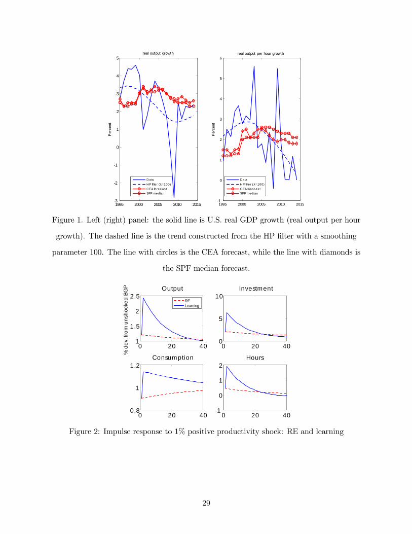
This section presents forecasts of the long-run growth of real gross domestic product (GDP)
and real output per hour. In the left panel of figure 1, the solid line is the U.S. annual real
GDP growth from 1995 to 2014. The dashed line is a proxy of the actual long-run GDP
growth constructed by applying the HP filter with a smoothing parameter of 100.2 Two
proxies for real-time forecasts of long-run output growth are also plotted. One proxy is the
real-time potential output growth estimates prepared by the U.S. Council of Economic Ad-
visors (CEA), reported in its annual Economic Report of the President (ERP) and published
in January (or February) of each year.3 The other proxy is the median forecast in the Survey
of Professional Forecasters (SPF) for the annual average rate of growth of real GDP over
the next 10 years published in February of each year. The right panel plots the same (four)
times series for real output per hour growth.4
The observed forecasts suggest gradual recognition and learning of the long-run growth of
2Edge, Laubach and Williams (2007) use this method to construct the trend growth of U.S. labor pro-ductivity. The results obtained in Table 1 are robust to a wide range of choices of the smoothing parameter.
3Potential output growth is viewed as output growth in the long-run. Therefore, the CEA also regardsthe estimates as the long-run growth forecasts in the annual ERP. 1995 is chosen as the starting year becausethe ERPs are available online from this year onwards.
4In the right panel of figure 1, the real output per hour is nonfarm business sector real output per hourfrom the FRED database. “CEA forecast”is the CEA forecast for trend productivity growth (measured bynonfarm business sector real output per hour). SPF simply asks “productivity.”
5
output and output per hour. In addition, observed forecasts for the long-run growth of real
GDP and real output per hour display systematic one-sided errors. During the late 1990s and
early 2000s, there was an acceleration of long-run real output growth and long-run output
per hour growth, while agents only gradually revised their growth expectations upward
and persistently underpredicted the long-run GDP growth. Thereafter, there was a period
of slower long-run growth; agents only gradually revised the long-run growth expectations
downward and persistently over-predicted the long-run growth. The autocorrelation for
forecast error of long-run real GDP growth is 0.95 for SPF median forecasts and 0.96 for
CEA forecasts, while for long-run real output per hour it is 0.94 for SPF median forecasts
and 0.98 for CEA forecasts; see Panel A of Table 1.
The flip side of very persistent long-run growth estimation error is the strongly positive
autocorrelation of output gap revisions. Edge and Rudd (2012) find that the Federal Re-
serve’s Greenbook revision in output gap —defined as the difference between the final and
real-time gap estimates —has an autocorrelation coeffi cient on the order of 0.9 during 1996-
2006. They show that this auto-correlation coeffi cient measure is robust to a wide range of
univariate detrending approaches and to different choices of time periods; see page 5 and
Table 3 of their paper. They suggest this points to gradual learning of the economy’s trend
growth by the Federal Reserve.
2.2 Comovement Between Long-Run Growth Forecasts and Cycli-
cal Activities
This section documents—to our knowledge for the first time—the comovement between long-
run growth expectations and cyclical activities. Panel B of Table 1 reports the correlation
between long-run real GDP growth expectations (SPF forecasts) and detrended real output,
investment, consumption and working hours, while Panel C reports the same correlations
6

using long-run output per hour growth forecasts.5 Three detrending methods are considered:
linear, quadratic detrending and HP filter with smoothing parameter 100.
There is a positive correlation between long-run output growth expectations and cyclical
activities; the corresponding correlation coeffi cient for output is 0.49 − 0.75, consumption
0.31 − 0.82, investment 0.46 − 0.74, and hours 0.30 − 0.59, depending on the detrending
methods. Similarly, the correlation between long-run output per hour growth forecasts and
cyclical activities is positive; the corresponding correlation coeffi cient for output is 0.48−0.70,
consumption 0.57−0.71, investment 0.47−0.58, and hours 0.22−0.38.6 The long-run growth
forecasts tend to be high during expansions, and contrariwise during contractions.
2.3 Short-Term Forecasts
The short term forecast errors from SPF display a similar systematic pattern documented in
e.g., Eusepi and Preston (2011). They show, for example, the median agent tends to under-
predict interest rates and overpredict unemployment over expansions, and contrariwise dur-
ing contractions. Online Appendix A1 shows that the median agent tends to under-predict
real output growth over expansions and contrariwise during contractions using 1-quarter
ahead forecast data. Panel D of Table 1 reports the autocorrelation of median 1-quarter
forecast errors for real GDP growth, two measures of interest rates, and unemployment, all
of which display a positive correlation.7
5Data is from the Bureau of Labor Statistics. Output is real GDP. Nominal consumption is con-structed as the sum of nondurable goods, services, and government expenditures. Nominal invest-ment is calculated as the sum of private residential investment, equipment and software, and con-sumption durable goods. Nominal consumption and investment are deflated by using the GDP de-flator. For hours, we use the data of total hours in Hall (2014) from 1989-2013 available athttp://web.stanford.edu/~rehall/Recent_Unpublished_Papers.html.
6Positive correlations are robustly produced between long-run output (or output per hour) growth fore-casts and all four detrended variables (output, consumption, investment and hours) for all three detrendingmethods under consideration using CEA forecasts.
7Using real time data, the autocorrelation of errors in 1, 2, 3 and 4-quarter-ahead real GDP growthforecasts are 0.23, 0.35, 0.36 and 0.38.
7

3 Model Setup
Our model is a standard RBC model with four main features: King-Plosser-Rebelo (KPR)
non-separable preferences between consumption and leisure, constant returns to scale tech-
nology, variable capital utilization, and a random walk with drift productivity process.
Households have KPR non-separable preferences between consumption and leisure which
is consistent with a balanced growth path; see eg. King and Rebelo (1999).8 The represen-
tative household maximizes
Et
∞∑t=0
βtu(Ct, Lt); u(Ct, Lt) =C1−σt v(1− Lt)
1− σ
subject to the flow budget constraint
Ct +Kt+1 = RKt (UtKt) +WtHt + (1− δ(Ut))Kt.
Et denotes the subjective expectations of agents for the future, which agents hold in the
absence of RE. RE analysis is standard. Ct, Lt, Ht, Kt, Ut are consumption, leisure, hours,
capital and capacity utilization rate. Wt and RKt are the wage rate and rental rate for capital
services. β is the discount rate between 0 and 1. σ > 1 and v′, v′′> 0. Capacity utilization
in the data displays pronounced procyclical variability (see King and Rebelo (1999)) and
is used to improve the fit of the model. Capital depreciation is assumed to increase with
capacity utilization Ut according to the function δ(Ut) = θ−1U θt where θ > 0.
There are a continuum of identical competitive firms of mass one. Each produces the
economy’s only good Yt using capital Kt and labor Ht as inputs according to the production
function
Yt = (UtKt)α(XtHt)
1−α (1)
8Households are assumed to have the same preferences and constraints, firms the same technology, andbeliefs are homogenous across agents (though no agent is assumed to be aware of this); hence, in what followswe do not distinguish explicitly between individual agents and firms.
8
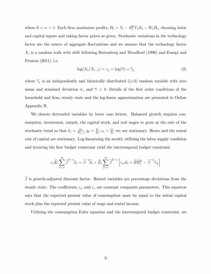
where 0 < α < 1. Each firm maximizes profits, Πt = Yt − RKt UtKt −WtHt, choosing labor
and capital inputs and taking factor prices as given. Stochastic variations in the technology
factor are the source of aggregate fluctuations and we assume that the technology factor
Xt is a random walk with drift following Rotemberg and Woodford (1996) and Eusepi and
Preston (2011), i.e.
log(Xt/Xt−1) = γt = log(γ) + γt (2)
where γt is an independently and identically distributed (i.i.d) random variable with zero
mean and standard deviation σγ and γ > 0. Details of the first order conditions of the
household and firm, steady state and the log-linear approximation are presented in Online
Appendix B.
We denote detrended variables by lower case letters. Balanced growth requires con-
sumption, investment, output, the capital stock, and real wages to grow at the rate of the
stochastic trend so that kt = Kt
Xt−1, yt = Yt
Xt, ct = Ct
Xtetc are stationary. Hours and the rental
rate of capital are stationary. Log-linearizing the model, utilizing the labor supply condition
and iterating the flow budget constraint yield the intertemporal budget constraint
εcEt
∞∑T=t
βT−t
cT = β−1kt + Et
∞∑T=t
βT−t [
εwwt + RRKt − β
−1γT
]
β is growth-adjusted discount factor. Hatted variables are percentage deviations from the
steady state. The coeffi cients εw and εc are constant composite parameters. This equation
says that the expected present value of consumption must be equal to the initial capital
stock plus the expected present value of wage and rental income.
Utilizing the consumption Euler equation and the intertemporal budget constraint, we
9
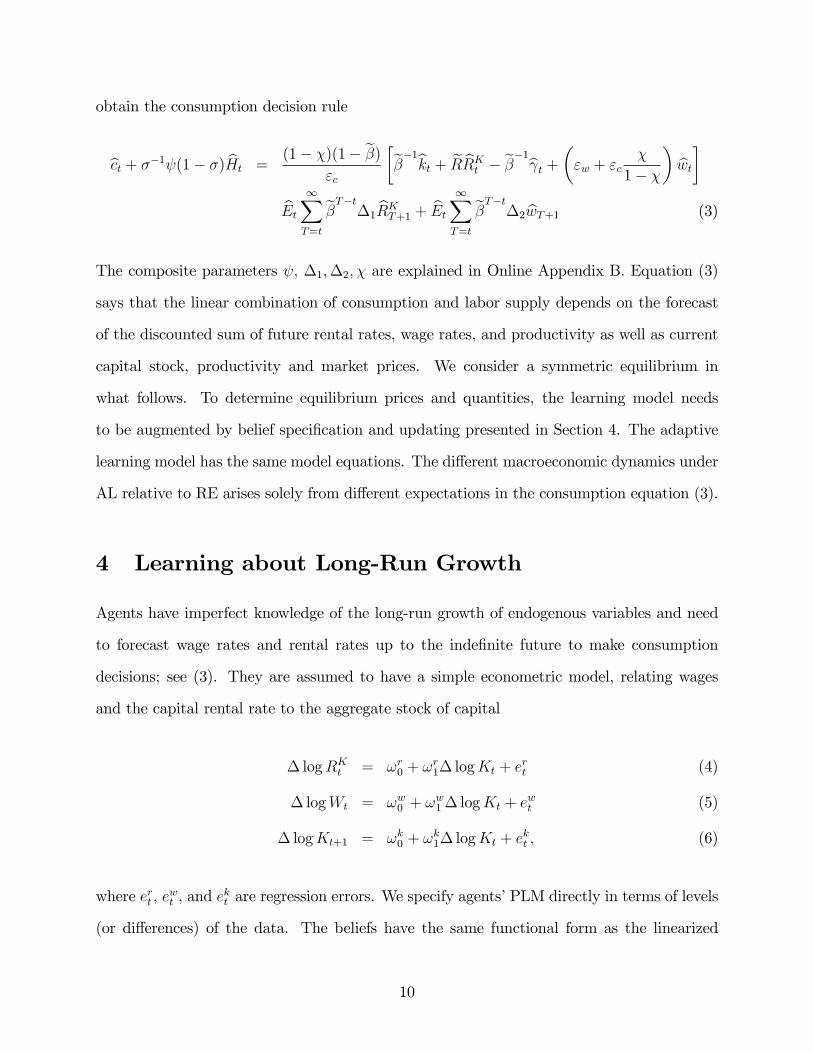
obtain the consumption decision rule
ct + σ−1ψ(1− σ)Ht =(1− χ)(1− β)
εc
[β−1kt + RRK
t − β−1γt +
(εw + εc
χ
1− χ
)wt
]Et
∞∑T=t
βT−t
∆1RKT+1 + Et
∞∑T=t
βT−t
∆2wT+1 (3)
The composite parameters ψ, ∆1,∆2, χ are explained in Online Appendix B. Equation (3)
says that the linear combination of consumption and labor supply depends on the forecast
of the discounted sum of future rental rates, wage rates, and productivity as well as current
capital stock, productivity and market prices. We consider a symmetric equilibrium in
what follows. To determine equilibrium prices and quantities, the learning model needs
to be augmented by belief specification and updating presented in Section 4. The adaptive
learning model has the same model equations. The different macroeconomic dynamics under
AL relative to RE arises solely from different expectations in the consumption equation (3).
4 Learning about Long-Run Growth
Agents have imperfect knowledge of the long-run growth of endogenous variables and need
to forecast wage rates and rental rates up to the indefinite future to make consumption
decisions; see (3). They are assumed to have a simple econometric model, relating wages
and the capital rental rate to the aggregate stock of capital
∆ logRKt = ωr0 + ωr1∆ logKt + ert (4)
∆ logWt = ωw0 + ωw1 ∆ logKt + ewt (5)
∆ logKt+1 = ωk0 + ωk1∆ logKt + ekt , (6)
where ert , ewt , and e
kt are regression errors. We specify agents’PLM directly in terms of levels
(or differences) of the data. The beliefs have the same functional form as the linearized
10
minimum-state-variable RE solution to the model (reformulated in levels). In the RE so-
lution, ωr0 = −ωr1 log γ, ωw0 = (1 − ωw1 ) log γ, ωk0 = (1 − ωk1) log γ, ωr1 = ωr1, ωw1 = ωw1 , ω
k1 =
ωk1, ert = −ωr1γt, ewt = (1 − ωw1 )γt, and e
kt = (1 − ωk1)γt where bar coeffi cients denote RE
values.9
Let ωi′
= (ωi0, ωi1) for i = r, w, k. zrt = ∆ logRK
t , zwt = ∆ logWt, z
kt = ∆ logKt+1, and
q′t−1 = (1,∆ logKt) . Beliefs at period t, ωit are updated recursively by the constant-gain
Generalized Stochastic Gradient (GSG) learning algorithm as in Evans, Honkapohja and
Williams (2010, henceforth EHW)
ωit = ωit−1 + giΓqt−1
(zit − ωi
′
t−1qt−1
)′(7)
where ωit denotes the current-period’s coeffi cient estimate.10 Γ controls the direction of belief
updating and gi ∈ (0, 1) , the constant gain, determining the rate at which older observations
are discounted. Bayesian and robustness justification for the GSG algorithm are provided in
EHW. In particular, they show that (1) GSG learning algorithm asymptotically approximates
the Bayesian optimal estimator when agents allow for drifting coeffi cients models, and (2)
it is also the “maximally robust”estimator when agents allow for model uncertainty. As is
standard in the literature, beliefs at t are updated using data up to period t− 1.
Analogous to (4) — (6), agents are assumed to have the following PLM for aggregate
output and output per hour
∆ log Yt = ωy0 + ωy1∆ logKt + eyt (8)
∆ log (Yt/Ht) = ωpr0 + ωpr1 ∆ logKt + eprt (9)
9It can be shown that ωr1, ωw1 , and ω
k1 are exactly the corresponding coeffi cients in the detrended and
linearized RE solution for rental rates, wage rates and capital.10An alternative learning rule is the constant-gain recursive least squares (CG-RLS) algorithm. Online
Appendix C4 shows that the impulse response functions of our model with CG-RLS learning are similarto the results with GSG learning. However, CG-RLS learning often imposes a projection facility on beliefsand/or generates singularity problem in inverting the moment matrix; this is perhaps not fully desirable andwe prefer presenting our results with GSG learning where the projection facility is not invoked.
11

where eyt and eprt are regression errors. They relate output and output per hour to capital as
under RE. The forecast of long-run growth of output and output per hour are related to the
forecast of the long-run growth of capital. They can be obtained by taking unconditional
expectations of equations (6), (8), and (9) and combining the resulting equations; Online
Appendix D1 provides the analytical formula.
5 Quantitative Results
This section evaluates the empirical performance of our learning model and contrasts it with
that of the full-information RE model.
5.1 Calibration
The model is calibrated to the postwar US data. The business cycle data statistics are taken
from Eusepi and Preston (2011) and their Appendix provides a description. The discount
factor β is set to 0.99, the capital share α to 0.34, the depreciation rate δ to 0.025 and the
unconditional mean of productivity growth γ to 1.0053. The inverse of Frisch elasticity of
labor supply is 0.1. The standard deviation of productivity shock σγ is calibrated to match the
standard deviation of HP-filtered output volatility. The parameter σ in the utility function
is chosen to match the consumption growth volatilities and set to 1.9. Evidence on observed
forecasts is used to discipline the choice of the gain parameter in line with Eusepi and Preston
(2011). The gain parameters gk and gw are set to 0.014 and gr to 0.03. The larger gain
parameter gr compared to gk and gw may be justified by the smaller measurement error (or
larger signal-noise ratio) in interest rates vis-a-vis capital and wage rates.11 The moment
matrix in (7) is set to the identity matrix, corresponding to the classical Stochastic Gradient
(SG) algorithm.12 Online Appendix C presents the quantitative results to alternative values
11Branch and Evans (2011) use heterogenous gain parameters in their learning model of stock marketbubbles and crashes.12Adopting the Bayesian interpretation of the GSG algorithm, Evans, Honkaphoja and Williams (2010),
p. 240, indicate that the choice of the perceived parameter innovation covariance V = γ2σ2Mz (in their
12

of the labor supply elasticity, gain parameter, moment matrices in the GSG learning rule
and the constant-gain recursive least squares learning rule.
5.2 Impulse Response Functions
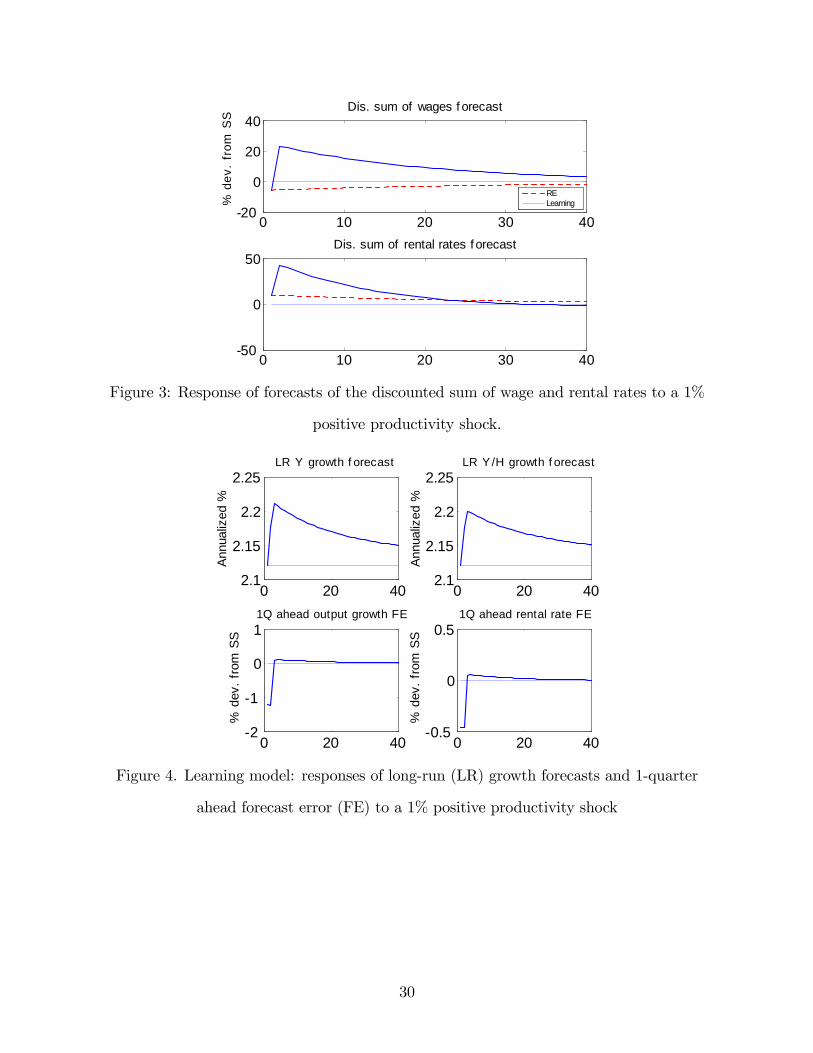
Figure 2 depicts the impulse response functions under RE and learning for 40 quarters in
response to a 1% positive productivity shock. For stationary variables, percentage deviations
from the steady state are plotted, while percentage deviations from the unshocked balanced
growth path are reported for nonstationary variables. For the learning model, agents’initial
beliefs are set equal to the corresponding RE values, which yields identical impact response
of the learning model as under RE.13
Under RE, there is a shortfall of capital after the shock. This raises the marginal product
of capital and hence the real interest rate. This implies the marginal utility of consumption
must fall over time. Capacity utilization rises on impact due to the increase in rental rates.
Output rises initially because working hours, capacity utilization and productivity increase
initially. The high interest rates induce people to postpone their consumption and leisure
and both variables increase over time. Output, on the other hand, decreases over time: this
is because capacity utilization and working hours decrease over time and this is suffi ciently
pronounced to offset the effect on output from the rise in capital stock.
The improvements in the learning model arise from belief revisions and the interplay of
beliefs and market outcomes. After the impact period, high realization of rental rates and
wage rates leads to upward revision of the forecasts for the discounted sum of wage and rental
notation) yields classical SG learning. They show that the SG learning algorithm is not scale invariant (pp.260-261). This is because when they change the units of regressors, they do not change the correspondingprior of the perceived variance covariance matrix V = γ2σ2Mz. However, the prior should be suitablyadjusted to V = γ2σ2Mz in response to a change in the units of regressors. The quantitative results of ourlearning model are then scale invariant and remain exactly the same in response to a change in the units ofregressors.13We note that the difference between median of the stationary distribution of agents’ beliefs and the
corresponding RE values is very small. We use a relative measure ie. median belief minus the correspondingRE value divided by the RE value to measure this difference. This relative measure for the intercept termof the capital equation and rental rates equation are about 1%. And for the remaining four coeffi cients inagents’PLM, this measure is smaller than 0.1%. The median and mean of the stationary distribution of thebeliefs are also very close.
13
rates, as can be seen in figure 3. The optimism about future wage rates helps to produce a
further rise in consumption. Working hours increase as firms’labor demand increases and
the constant-consumption labor supply shifts rightward. The increase in the return to capital
due to rising productivity and working hours induces an increase in investment. Output also
rises due to increases in productivity, working hours, investment and capacity utilization.
At some point, the realized wage rate growth falls short of their forecasts and they start
revising their belief of wage rate growth downward. Associated with the downward belief
revision is a decline in consumption and other aggregate activities. The mutual influence of
agents’expectations and equilibrium outcomes yields a decline in aggregate activities.
Rotemberg and Woodford (1996) demonstrated basic RE business cycle models (with-
out variable utilization rates of capital) do not generate the positive comovement between
consumption (C), investment (I), hours (H), and output (Y) in the data. Our RE model
with variable capacity utilization confirms the same finding in Figure 2. In contrast, Fig-
ure 2 shows that there is positive comovement between C, I, H and Y under learning after
impact. Moreover, learning strongly amplifies the response of output, hours and investment
and improves the internal propagation of the model evident in the persistent rise and fall of
the four variables.
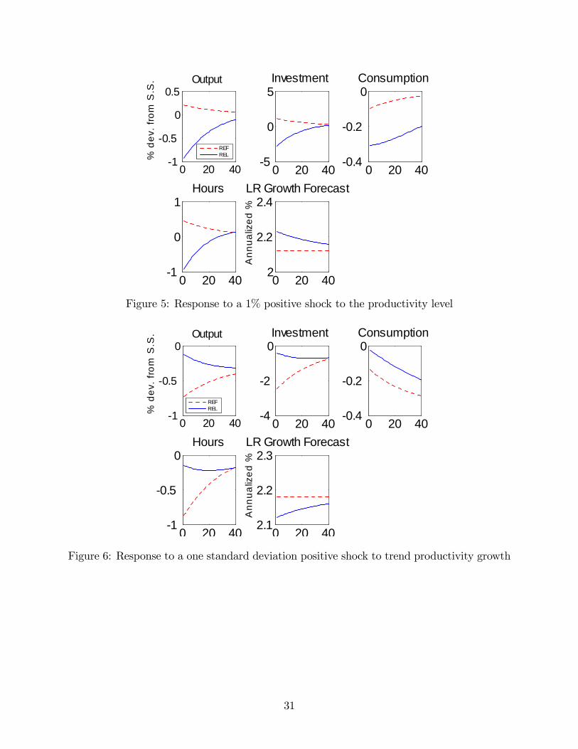
Figure 4 plots impulse response of long-run growth forecasts for output and output per
hour on the top panel and 1-quarter ahead forecast error for output growth and rental rates in
response to the productivity shock. The two long-run growth forecasts rise for several periods
and then converge towards the RE value. Figures 2 and 4 suggest a positive correlation
between long-run growth forecasts and cyclical activities. The 1-quarter ahead forecast
errors —defined as the forecasts from the previous period minus the outturns —for output
and rental rates become negative following the shock and are positively autocorrelated.
14
5.3 Statistical Properties
To compare with postwar US data, we calculate business cycle statistics based on 162 quar-
ters. The learning model is simulated for 2000 + 162 periods and 500 repetitions. The first
2000 periods are used to generate the stationary distribution of beliefs and the final 162
periods are used to calculate the business cycle statistics. Median statistics are reported
along with the standard deviations in the parenthesis. The learning model is stable and no
projection facility is used in producing the statistics.
Panel A of Table 2 compares the autocorrelation of long-run and short-term forecast
errors in the data and in the learning model. The learning model quantitatively matches
well the autocorrelation of the long-run growth forecast error and produces somehow higher
autocorrelation of 1-quarter ahead forecast error for GDP growth and real interest rate.14
The mutual influence of beliefs and market outcomes in the learning model also produces a
positive correlation between the long-run growth forecasts of output (or output per hour)
and HP-filtered output, hours, consumption, and investment present in the data (refer to
Panel B and C of Table 2).
Table 3 reports major business cycle statistics. Recall that the standard deviation of the
productivity shocks is chosen to match the HP-filtered output volatility in the data. This
results in a standard deviation of productivity of 0.52% in the learning model and 0.99%
in the RE model i.e. the learning model requires 47% smaller standard deviation of the
productivity shocks. The standard deviation of hours and investment relative to output is
119% and 50% higher in the learning model and is closer to that in the data.
Burnside, Eichenbaum, and Rebelo (1996, henceforth BER) reported 0.131 as the relative
volatility of productivity shocks (measured by the Solow residuals associated with the US
manufacturing sector during 1972-1992) to output after correcting for capital utilization, see
14The errors in long-run growth forecast are computed here as the forecasts minus the constant log(γ).Strong autocorrelation of long-run growth forecast errors is due to slow convergence of the growth beliefs;see the top panels of Figure 4. Alternatively, the long-run growth forecast errors can be calculated as theforecasts minus the HP-filtered trend output growth, which gives similar results; the median autocorrelationof long-run growth forecast errors for both output and output per hour is 0.99.
15

their Table 1. This suggests a 70% drop in the volatility of the growth rate of productivity
shocks relative to output than the number used in the basic RBC model; so a successful
model must display much stronger amplification than the basic RBC model. Our learning
model can produce strong amplification of productivity shocks; this ratio in the learning
model is 0.143 and close to the BER estimate.15
Panel B of Table 3 reports autocorrelation in the growth rates of C, I, Y, H and pro-
ductivity. The RE model generates almost no propagation of the productivity shock; in
particular, it does not generate the degree of autocorrelation of output growth present in the
data as pointed out by Cogley and Nason (1995). As is evident from this table, a similar
comment applies to the growth of C, I, H and productivity. The learning model generates
strong propagation and produces somehow higher autocorrelation of the growth rates data.
The first-order autocorrelation of output growth is 0.48 in the learning model (in contrast
to 0.30 in the data); this positive autocorrelation arises from belief revision and the inter-
action of beliefs and market outcomes evident in the impulse response functions in Figure
2. The learning model also generates strong propagation in other variables including labor
productivity.
Panel C and D report the business cycle statistics using data on growth rates. The
learning model delivers a good fit to the volatility of output growth and other relative
standard deviations, such as investment and hours growth volatilities. It also generates
significantly better correlation between productivity growth and output growth ρ∆ Pr,∆Y and
between productivity growth and hours growth ρ∆ Pr,∆H .16
15The counterpart to the total factor productivity (TFP) shocks in BER (1996) in our model is (1− α)γtwith α = 0.34. The standard deviation of the growth rate of productivity shocks and output in our model is0.52% and 3.62%/4. So the ratio of the volatility of the growth of TFP to output is (1− 0.34)
2 (0.52%)2
(3.62%/4)2=
0.143.16Online Appendix D2 reports correlations of HP-filtered data and Appendix C shows that the quantitative
results are robust to alternative parameterizations of the model and learning rules.
16
6 Knowledge About Trend in RE Models
This section shows existing full-information and imperfect information RE models cannot
produce the facts reported in sections 2.1 and 2.2. The productivity process (2) is augmented
as
log(Xt/Xt−1) = log(γt) + γt (10)
log(γt) = (1− ργ) log(γ) + ργ log(γt−1) + γt. (11)
ργ is in (−1, 1], γt are i.i.d shocks to trend growth rates and log(γ) is the unconditional mean
of the trend growth rates. Most RE models assume ργ = 0 and γt = 0 which reduces to our
process (2) eg. King and Rebelo (1999). The formulation (10)-(11) allows for time-varying
and persistent trend growth rates as in e.g. Aguiar and Gopinath (2007) and Edge, Laubach
and Williams (2007).
Section 6.1 (Section 6.2) shows that existing full information and imperfect information
RE models with |ργ| < 1 (ργ = 1) produce counterfactually zero (negative) correlation
between long-run growth forecasts and cyclical activities, which is inconsistent with the
evidence in Section 2.2.
6.1 Mean-Reverting Trend Growth (|ργ| < 1)
In full-information models e.g., Aguiar and Gopinath (2007), agents can observe productivity
growth and its trend component. They have suffi cient information —such as the knowledge
of other agents’ beliefs, preferences and technology — to derive the equilibrium mapping
from the trend growth of exogenous variables (e.g. productivity) to the trend growth of
endogenous variables (e.g. output, output per hour); they know exactly the law of motion of
endogenous variables and their long-run growth. These RE models (with or without time-
varying trend growth) are inconsistent with the facts documented in Section 2.1 and 2.2
because (1) agents’ long-run output (and output per hour) growth forecasts are constant
17
(log(γ)) and do not display systematic errors, (2) the correlation between long-run growth
forecasts and cyclical activities is zero.17
Another class of models assume agents have less information and cannot observe the trend
growth rates of the exogenous (productivity) process, such as Edge, Laubach and Williams
(2007) and Boz, Daude, and Durdu (2011). Agents face a signal extraction problem; they use
the new observation of productivity to update their trend growth beliefs. However, agents in
these models are endowed with the knowledge of ργ and log(γ), so their long-run productivity
growth forecasts are constant (log(γ)) over time. Since agents know the equilibrium mapping
from long-run productivity growth to long-run output (and output per hour) growth, all these
growth forecasts are equal to log(γ). These models also produce zero correlation between
long-run output (or output per hour) growth forecasts and cyclical activities. Moreover, as
a consequence of RE, the long-run growth forecast errors in endogenous variables will not
display a systematic pattern, which is inconsistent with the evidence in Section 2.1.
6.2 Random Walk Trend Growth (ργ = 1)
We now show that in the case ργ = 1 (e.g. considered in Edge, Laubach and Williams
(2007)), full-information and imperfect information RE models produce a negative correla-
tion between long-run output (or output per hour) growth forecasts and cyclical activities.
Agents update their trend growth beliefs via a constant-gain learning rule (or equivalently the
Kalman filter with steady state updating coeffi cients) log(γt) = log(γt−1)+gx(log(Xt/Xt−1)−
log(γt−1)). Economic decisions are based on their beliefs about the trend productivity growth.
For illustration, the gain parameter gx is set to 0.11/4 as in Edge, Laubach, and Williams
(2007). The standard deviation of γt is set to 0.52% as in our adaptive learning model; the
standard deviation of the shock to long-run growth rate is set to 0.015% implied by the
chosen gain. All other parameters are identical to those in our benchmark setting. (Similar
17These comments also apply to full-information RE models which do not explicitly model the trendcomponent but start directly with detrended variables or the cyclical component. This is because implicitly,agents in these models also have exact knowledge about the law of motion for the trend.
18

shapes of IRFs are found for alternative values of gain parameters.). The long-run growth
forecasts for productivity, output and output per hour are the same due to agents’exact
knowledge of the equilibrium mapping.
Figure 5 reports the response of detrended variables (measured as percentage deviations
from the steady state) and the annualized long-run growth forecasts to a positive 1% shock
to the level of productivity. The full-information model is labeled “REF”and the imperfect
information model is labeled “REL”. The REF model produces constant long-run growth
forecasts and zero correlation between the forecasts and detrended variables; the level shock
does not change long-run growth forecasts. In the REL model, long-run growth forecasts
are not constant. The positive shock leads to an upward revision of the long-run growth
forecasts. The impact response of Y, I, C, and H are smaller in the REL model relative
to REF due to higher long-run growth expectations and larger wealth effects on leisure.
Associated with a rise in the long-run growth forecasts is a decline in Y, I, C, and H. After
the impact period, agents revise their long-run growth forecasts down. Associated with this
downward belief revision is rising Y, I, C, and H. This suggests negative comovement between
long-run growth forecasts and detrended macro variables.
Our adaptive learning model is better able to reproduce the relevant business cycle volatil-
ities than the RELmodel mainly due to the feedback frommarket outcomes to agents’beliefs.
Comparing Figure 2 with Figure 5, the amplitude of the response of output, investment, and
hours in our adaptive learning model is 54%, 90% and 108% larger than the corresponding
numbers of the REL model.
Figure 6 displays the response to a positive one standard deviation shock to trend pro-
ductivity growth. Under REF, (detrended) Y, I, C, H decline a lot due to the large wealth
effects in the impact period, while long-run growth forecasts increase on impact. The fore-
casts stay constant afterwards associated with which are rising Y, I, C, H. Again these
suggest a negative correlation between long-run growth forecasts and detrended variables.
Under REL, long-run growth forecasts increase much less initially relative to REF and as
19

a consequence, cyclical aggregate activities decline by less. There is negative comovement
between the long-run growth forecasts and detrended variables.
Before concluding this section, we remark that shocks to trend productivity growth, as
eg. in (10)-(11), are not required by our learning model (presented in Section 4) to generate
the high autocorrelation in trend growth rates of output and output per hour evidenced
in the data. Our model with zero correlation in trend productivity growth endogenously
generates an autocorrelation coeffi cient of 0.99 and 0.996 for trend output growth and trend
output per hour growth respectively, using HP-filtering; the corresponding numbers in the
data are 0.99 and 0.984 (see e.g. Figure 1).
7 Adaptive Learning (AL) Models
This section shows that the belief specification in existing AL business cycle models imply
that agents have exact knowledge of the trend growth of endogenous variables (as under RE).
Therefore, these models produce constant long-run growth forecasts and zero correlation
between long-run growth forecasts and cyclical activities, which appear inconsistent with
the observed forecasts.
AL modelers make weaker informational assumptions with agents having incomplete
knowledge of the structure of the economy analyzing macroeconomic policy and their em-
pirical implications, such as Bullard and Mitra (2002), Evans and Honkapohja (2003), and
Eusepi and Preston (2011). These models assume agents only learn detrended variables and
typically the parameter coeffi cients in the detrended and linearized RE solution. Take the
following perceived law of motion (PLM) as an example
RKt = ωr0 + ωr1kt + ωr3γt + ert , (12)
wt = ωw0 + ωw1 kt + ωw3 γt + ewt , (13)
kt+1 = ωk0 + ωk1kt + ωk3γt + ekt ; (14)
20
ω′s are agents’ belief parameters and ert , ewt , and ekt are regression errors.
18 Under RE,
ωr0 = ωw0 = ωk0 = 0 and ert = ewt = ekt = 0; ω′1s and ω
′2s are RE coeffi cients. Under adaptive
learning, agents are uncertain and learn about ω′s. The intercept terms in (12)-(14) can be
interpreted as agents’uncertainty about the non-stochastic steady state or the level of the
trend component (in contrast to exact knowledge of the level of the trend under RE).
We reformulate (12)-(14) in levels and perform the Beveridge and Nelson (1981) decom-
position for log rental rates, wage rates, and capital. logZPt denotes the trend component of
variable logZt.
Proposition 1 The belief specification (12)-(14) implies that households’perceived law of
motion for the trend component of log rental rates, wage rates, and capital are
log(RKt )P − log(RK
t−1)P = 0 (15)
logW Pt − logW P
t−1 = log γ + γt (16)
logKPt+1 − logKP
t = log γ + γt (17)
Online Appendix E provides the proof. Agents know exactly the trend growth rate
of rental rates, wage rates, and capital, including not only the deterministic but also the
stochastic component. The growth component of trend wage rates and capital, i.e., the right
hand sides of (16) and (17), are identical to the growth component of the productivity process,
i.e., the right hand side of (2). To emphasize, they know that the unconditional mean growth
rate of wages and capital is identical to that of the productivity process. Moreover, they also
know precisely how a shock to the productivity (γt) affects the evolution of the permanent
component of wages and capital (i.e. they know that the coeffi cient of γt is 1!). The growth
component of rental rates, i.e., the right hand side of (15) is zero; this implies that agents
know that the permanent component log(RKt )P is constant over time and hence that log(RK
t )
is stationary. Beyond knowing that some endogenous variables are stationary and that the18Eusepi and Preston (2011) and Huang, Liu and Zha (2011) use similar formulations; the latter assumes
that agents only learn about the steady state of capital i.e. ωk1 = ωk3 = 0.
21

rest non-stationary, the belief specification (12)-(14) implies that agents know the existence
of a balanced growth path. In particular, agents are aware that the non-stationary variables
share a common trend which is equal to the growth rate of productivity.19 Online Appendix
F provides a graphic illustration on how our learning model is conceptually different from the
formulation of learning with detrended data and with the full-information RE benchmark.
Given agents’exact knowledge of the trend growth, it follows that the long-run output
(and output per hour) growth forecasts in these AL models will be constant, i.e., log(γ) and
not correlated with cyclical activities.
8 Conclusion
Macroeconomic models used for analyzing economic fluctuations and welfare separate an
underlying growth path or trend from the cycle and assume agents have exact knowledge
of the law of motion for the trend component of endogenous variables including their long-
run growth. These models produce zero correlation between long-run growth forecasts and
cyclical activities and do not display systematic forecast errors in long-run growth. These
implications are inconsistent with observed forecasts which suggest a positive correlation be-
tween the long-run output (or output per hour) growth forecasts and cyclical activities and
strongly positive autocorrelation of the long-run growth forecast errors in output (and output
per hour). A simple RBC model with learning about the long-run growth of endogenous vari-
ables is developed. This model can produce these positive correlations and suggests a critical
role for shifting long-run growth expectations to understand business cycle fluctuations.
19The same arguments apply to models with under-parameterized PLMs, eg. Huang, Liu and Zha (2011)(see also Adam (2007) for an under-paramterized PLM in a sticky price model). The arguments also apply toAL models with over-parameterized PLMs and to Bullard and Duffy (2005) and Mitra, Evans and Honkapo-hja (2013) where agents learn the law of motion of (detrended) linearized variables rather than percentagedeviations from the non-stochastic steady state; see the proof in Online Appendix E.
22

References
Adam, K., (2007). Experimental evidence on the persistence of output and inflation.
Economic Journal 117, 603-636.
Adam, K., J., Beutel, and A., Marcet (2015). Stock Price Booms and Expected Capital
Gains. Mannheim University mimeo.
Adam, K., P., Kuang, and A., Marcet, (2012). House Price Booms and the Current
Account. NBER Macroeconomics Annual 26, 77 - 122.
Adam, K, A., Marcet (2011). Internal Rationality, Imperfect Market Knowledge and
Asset Prices. Journal of Economic Theory, 146, 1224-1252.
Adam, K., A., Marcet, and J.P., Nicolini (2015). Stock market volatility and learning.
Journal of Finance, forthcoming.
Aguiar, M., and G., Gopinath (2007). Emerging market business cycles: the cycle is the
trend. Journal of Political Economy 115, 69-102.
Beveridge, S., and C., Nelson (1981). A New Approach to Decomposition of Economic
Time Series into Permanent and Transitory Components with Particular Attention to Mea-
surement of the ‘Business Cycle’. Journal of Monetary Economics 7, 151-174.
Boz, E., C., Daude, and B., Durdu, (2011). Emerging Market Business Cycles: Learning
about the Trend. Journal of Monetary Economics 58, 616-631.
Branch, W., G., Evans (2011). Learning about Risk and Return: A Simple Model of
Bubbles and Crashes. American Economic Journal: Macroeconomics, 159-191.
Bullard, J., and J., Duffy (2005). Learning and Structural Change in Macroeconomic
Data. Federal Reserve Bank of St. Louis Working Paper 2004-016A.
Bullard, J., and K., Mitra (2002). Learning about Monetary Policy Rules. Journal of
Monetary Economics 49, 1105-1129.
Burnside, C., M., Eichenbaum, and S., Rebelo (1996). Sectoral Solow Residuals. Euro-
pean Economic Review 40, 861-869.
Cochrane, J. (1994). “Shocks,”in Carnegie-Rochester Conference Series on Public Policy,
23
41, December.
Cogley, T., and J., Nason, (1995). Output Dynamics in Real-Business-Cycle Models.
American Economic Review 85, 492-511.
Edge, R., T., Laubach, and J., Williams, (2007). Learning and Shifts in Long-Run
Productivity Growth. Journal of Monetary Economics 54, 2421-2438.
Edge, R., and J., Rudd (2012). Real-Time Properties of the Federal Reserve’s Output
Gap. FRB Finance and Economics Discussion Series no. 86.
Eusepi, S., and B., Preston (2011). Expectations, Learning and Business Cycle Fluctua-
tions. American Economic Review 101(6): 2844-72.
Evans, G., and S., Honkapohja, (2003). Expectations and the Stability Problem for
Optimal Monetary Policy. Review of Economic Studies 70, 807-824.
Evans, G., S., Honkapohja, and N., Williams (2010). Generalized Stochastic Gradient
Learning. International Economic Review 51, 237-262.
Hall, R., (2014). Secular Stagnation. Stanford university mimeo.
Huang, K., Z., Liu, and T., Zha, (2009). Learning, Adaptive Expectations, and Technol-
ogy Shock. Economic Journal 119, 377-405.
King, R. G. and S. Rebelo (1999). Resuscitating Real Business Cycles. Handbook of
Macroeconomics, Chapter 14, Volume 1, 927-1007.
Kocherlakota, N. (2009). Mordern Macroeconomic Models as Tools for Economic Policy.
2009 Annual Report Essay.
Mitra, K., G., Evans, and S., Honkapohja, (2013). Policy Change and Learning in the
Real Business Cycle Model. Journal of Economic Dynamics and Control 37, 1947-1971.
Preston, B. (2005). Learning About Monetary Policy Rules When Long-Horizon Expec-
tations Matter. International Journal of Central Banking, 1(2): 81—126.
Preston, B. (2006). Adaptive Learning, Forecast-based Instrument Rules and Monetary
Policy. Journal of Monetary Economics 53, 507-535.
Rotemberg, J., and M., Woodford, (1996). Real-Business-Cycle Models and the Fore-
24

castable Movements in Output, Hours, and Consumption. American Economic Review 86,
71-89.
25
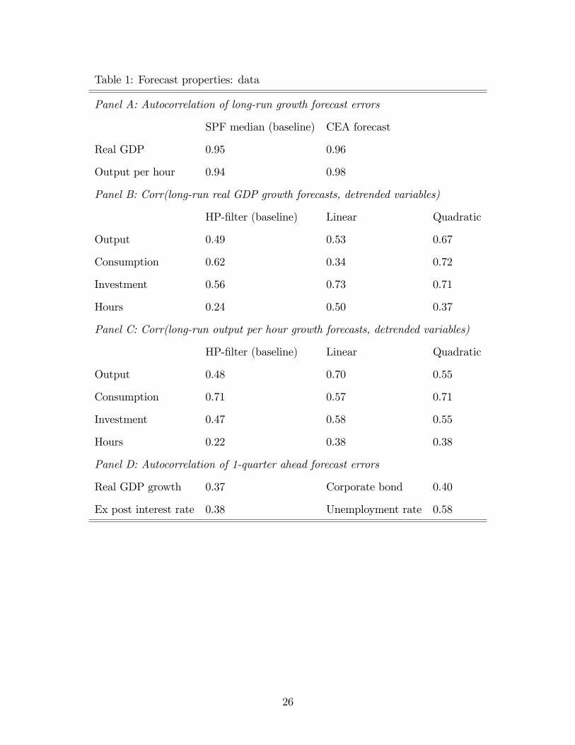
Table 1: Forecast properties: data
Panel A: Autocorrelation of long-run growth forecast errors
SPF median (baseline) CEA forecast
Real GDP 0.95 0.96
Output per hour 0.94 0.98
Panel B: Corr(long-run real GDP growth forecasts, detrended variables)
HP-filter (baseline) Linear Quadratic
Output 0.49 0.53 0.67
Consumption 0.62 0.34 0.72
Investment 0.56 0.73 0.71
Hours 0.24 0.50 0.37
Panel C: Corr(long-run output per hour growth forecasts, detrended variables)
HP-filter (baseline) Linear Quadratic
Output 0.48 0.70 0.55
Consumption 0.71 0.57 0.71
Investment 0.47 0.58 0.55
Hours 0.22 0.38 0.38
Panel D: Autocorrelation of 1-quarter ahead forecast errors
Real GDP growth 0.37 Corporate bond 0.40
Ex post interest rate 0.38 Unemployment rate 0.58
26

Table 2: Forecast properties: learning model and data
Data Learning Data Learning
Panel A: forecast error autocorrelation
Long-run output growth 0.95 0.97 Long-run Y/H growth 0.94 0.97
(0.02) (0.02)
Output growth 0.37 0.48 Real interest rate 0.38 0.48
(1Q ahead) (0.06) (1Q ahead) (0.06)
Panel B: Corr(long-run real GDP growth forecasts, detrended variables)
Output 0.49 0.47 Investment 0.56 0.47
(0.12) (0.12)
Consumption 0.62 0.44 Hours 0.24 0.47
(0.12) (0.12)
Panel C: Corr(long-run output per hour growth forecasts, detrended variables)
Output 0.48 0.45 Investment 0.47 0.46
(0.12) (0.12)
Consumption 0.71 0.43 Hours 0.22 0.45
(0.12) (0.12)
27

Table 3: Business Cycle Statistics
Data Model Data Model
RE Learning RE Learning
Panel A: (relative) standard Panel B: autocorrelation
deviation (HP-filtered data) (growth rates data)
σA - 0.99 0.52 ∆C 0.27 -0.00 0.24
σC/σY 0.55 0.75 0.47 (0.08) (0.07)
(0.00) (0.00) ∆I 0.35 -0.01 0.37
σI/σY 2.88 1.74 2.61 (0.08) (0.06)
(0.00) (0.01) ∆Y 0.30 -0.01 0.48
σH/σY 0.92 0.37 0.81 (0.08) (0.06)
(0.00) (0.01) ∆H 0.41 -0.01 0.25
σPr/σY 0.52 0.63 0.27 (0.08) (0.07)
(0.00) (0.01) ∆ Pr -0.06 0.00 -0.29
(0.08) (0.07)
Panel C: relative standard deviation Panel D: correlation
(growth rates data) (growth rates data)
σ4∆Y 3.96 4.76 3.62 ρ∆C,∆Y 0.5 1.00 0.85
(0.19) (0.25) (0.00) (0.02)
σ∆C/σ∆Y 0.55 0.75 0.53 ρ∆I,∆Y 0.74 1.00 0.95
(0.00) (0.01) (0.00) (0.01)
σ∆I/σ∆Y 2.56 1.74 2.73 ρ∆H,∆Y 0.68 1.00 0.89
(0.00) (0.03) (0.00) (0.02)
σ∆H/σ∆Y 0.8 0.37 0.91 ρ∆ Pr,∆Y 0.62 1.00 0.42
(0.00) (0.02) (0.00) (0.03)
σ∆ Pr/σ∆Y 0.74 0.63 0.46 ρ∆ Pr,∆H -0.16 0.99 -0.04
(0.00) (0.03) (0.00) (0.07)
28
1995 2000 2005 2010 20153
2
1
0
1
2
3
4
5
Per
cent
real output growth
D ataH P filter (λ=100)C EA forec as tSPF median
1995 2000 2005 2010 20151
0
1
2
3
4
5
6
Per
cent
real output per hour growth
D ataH P filter (λ=100)C EA forec as tSPF median
Figure 1. Left (right) panel: the solid line is U.S. real GDP growth (real output per hour
growth). The dashed line is the trend constructed from the HP filter with a smoothing
parameter 100. The line with circles is the CEA forecast, while the line with diamonds is
the SPF median forecast.
0 20 401
1.5
2
2.5
% d
ev. f
rom
uns
hock
ed B
GP Output
RELearning
0 20 400
5
10Investment
0 20 400.8
1
1.2Consumption
0 20 401
0
1
2Hours
Figure 2: Impulse response to 1% positive productivity shock: RE and learning
29
0 10 20 30 4020
0
20
40Dis. sum of wages f orecast
% d
ev.
from
SS
RELearning
0 10 20 30 4050
0
50Dis. sum of rental rates f orecast
Figure 3: Response of forecasts of the discounted sum of wage and rental rates to a 1%
positive productivity shock.
0 20 402.1
2.15
2.2
2.25LR Y growth f orecast
Ann
ualiz
ed %
0 20 402.1
2.15
2.2
2.25LR Y /H growth f orecast
Ann
ualiz
ed %
0 20 402
1
0
11Q ahead output growth FE
% d
ev.
from
SS
0 20 400.5
0
0.51Q ahead rental rate FE
% d
ev.
from
SS
Figure 4. Learning model: responses of long-run (LR) growth forecasts and 1-quarter
ahead forecast error (FE) to a 1% positive productivity shock
30
0 20 401
0.5
0
0.5Output
% d
ev.
fro
m S
.S.
REFREL
0 20 405
0
5Investment
0 20 400.4
0.2
0Consumption
0 20 401
0
1Hours
0 20 402
2.2
2.4LR Growth Forecast
An
nu
aliz
ed
%
Figure 5: Response to a 1% positive shock to the productivity level
0 20 401
0.5
0Output
% d
ev.
fro
m S
.S.
REFREL
0 20 404
2
0Investment
0 20 400.4
0.2
0Consumption
0 20 401
0.5
0Hours
0 20 402.1
2.2
2.3LR Growth Forecast
An
nu
aliz
ed
%
Figure 6: Response to a one standard deviation positive shock to trend productivity growth
31
Online Appendix (Not for publication)
A Output Growth Forecasts
Figure A.1 shows that the median agent tends to under-predict real output growth over
expansions and contrariwise during contractions using 1-quarter ahead forecast data.
B Model Details
This section provides first-order conditions, the steady state and log-linearzations of the
model. The variables with a bar are the non-stochastic steady state values while the vari-
ables with a hat denote log-linearized variables around the non-stochastic steady state i.e.
xt = log XtX. Capital letters denote levels while small case letters denote their stationary
counterparts.
Household optimization yields the following first-order conditions:
Ct : uC(Ct, Lt) = Λt
Kt+1 : βEtΛt+1RKt+1Ut+1 − Λt + βEt[Λt+1(1− δ(Ut+1)] = 0
Lt : uL(Ct, Lt) = ΛtWt
Ut : RKt = δ′(Ut)
where Λt is the Lagrangian multiplier associated with period t budget constraint.
Steady State
From the consumption Euler equation we get
RkU
γ= γσ−1β−1 − 1− δ
γ
= β−1− 1− δ
γ
32

and from the capacity utilization first-order condition
RkU
γ=δθ
γ=> θ =
RkU
δ
which defines θ, allowing to determine U and therefore Rk. The ratios
y
k= (α)−1R
kU
γ;i
k= 1− 1− δ
γ;c
k=y
k− i
kand
c
y=c
k/y
k
Finally the steady state level ψ, for a given choice of H, is determined by
ψ =Hv
′(H)
v(H)(σ − 1)−1 =
wH
y
y
c= (1− α)
y
c
Equilibrium condition and log-linearization
Households’optimality conditions
1. Marginal utility of consumption
λt = −σct − ψ(1− σ)Ht (18)
where in steady state
ψ ≡ −Hv′(H)
v(H)(1− σ)−1 =
wH
c
2. Euler equation
βEt[β−1(λt+1 − λt − σγt+1) + (β−1 − 1− δ
γσ)(RK
t+1 + Ut+1)− δ
γσθUt+1] = 0
Substituting the steady-state relation into the above equation yields
RKU
γ=
(β−1 − 1− δ
γσ
)=θδ
γσ
33

becomes
βEt
[β−1(λt+1 − λt − σγt+1) + (β−1 − 1− δ
γσ)RK
t+1
]= 0 (19)
3. Labor-leisure choice:
(1− σ) ct + εvHt = λt + wt
which, combined with the expression for marginal utility, gives:
σ−1λt + wt = εHHt (20)
where
εH = εv −(σ − 1)2
σψ > 0
is the inverse Frisch elasticity of labor supply.
4. Capacity utilization
Ut =RKt
θ − 1
Using the expression for the marginal utility of consumption, the Euler equation becomes
λt = Et
[(λt+1 − σγt+1
)+ βRRK
t+1
]−σct − (1− σ)Ht = Et
[−σct+1 − (1− σ)Ht+1
]− σEtγt+1 + EtβRR
Kt+1
where
R =
(β−1 − 1− δ
γσ
)Firms’problem
The firms’problem is
maxUtKt,Ht
Yt −WtHt −RKt (UtKt)
34

subject to the production technology
Yt = (UtKt)α(XtHt)
1−α
The first order condition with respect to hours:
−Wt + (1− α) (UtKt)α(Xt)
1−αH−αt = 0
becomes
(1− α)Xαt−1
(Ut
Kt
Xt−1
)αX−αt = 0
and hence
(1− α)γ−αt (Utkt)αH−αt = wt
Combined with the definition of output gives
wt = (1− α)ytHt
which in log-linear form becomes
wt = yt − Ht (21)
The capital input decision gives:
0 = −RKt + α(UtKt)
α−1(XtHt)1−α
= −RKt + α(Ut
Kt
Xt
)α−1(Ht)1−α
= −RKt + α(
Utγtkt)
α−1(Ht)1−α
Using the definition of output yields
RKt = αγt
ytUtkt
35

which in log-linear form is
RKt = γt + yt − Ut − kt
Finally, the evolution of capital is
Kt+1 = (1− δ)Kt + It
The log-linearized version is
kt+1 =i
kit +
(1− δ)γ
(kt − γt
)− δθ
γUt
Market clearing requires
Yt = Ct + It
The log-linearized version is
yt =
(1− c
y
)it +
c
yct
To summarize, the system of log-linearized equations under RE is
wt −(εH −
σ − 1
σψ
)Ht − ct = 0
−wt + yt − Ht = 0
−RKt + yt − Ut −
(kt − γt
)= 0
−yt +
(1− c
y
)it +
c
yct = 0
−yt + (1− α) Ht + αUt + α(kt − γt
)= 0
−δθγUt − kt+1 +
i
kit +
(1− δ)γ
(kt − γt
)= 0
− RKt
θ − 1+ Ut = 0
(σct + (1− σ)Ht)− Et[((σct+1 + (1− σ)Ht+1)− σγt+1)] + βRRKt+1 = 0
36
Consumption Decision Rule
In our learning model, the last equation in the above system is replaced by the following
consumption decision rule
ct + σ−1ψ(1− σ)Ht =(1− χ)(1− β)
εc
[β−1kt + RRK
t − β−1γt +
(εw + εc
χ
1− χ
)wt
]Et
∞∑T=t
βT−t
∆1RKT+1 + Et
∞∑T=t
βT−t
∆2wT+1,
which is identical to the last equation of page 7 in the Online Appendix of Eusepi and
Preston (2011) with ∆1 =
[(1−χ)(1−β)
εc− βσ−1
]βR and ∆2 =
(1−χ)(1−β)εc
β(εw + εc
χ1−χ
).20
Derivations and the definition of composite parameters ψ, χ, β, R, εw, εc are provided there.
C Robustness
This section provides robustness analysis of our model with alternative values of gain para-
meters, labor supply elasticity, alternative moment matrices in the GSG learning algorithm
and the constant gain recursive least squares (RLS) learning algorithm.21 In this section,
the standard deviation of the productivity shock in both the RE and our learning model are
set equal to 0.52% (as in our baseline learning model). As in the baseline learning model,
the projection facility is not used in generating statistics in this section.
C.1 Alternative gain parameters
Table A.1 demonstrates the empirical performance of the learning model under alternative
gain parameters spanning the interval (0.006, 0.017) for gw and gk and (0.017, 0.036) for gr.
Recall our baseline learning model has the gain parameter gw = gk = 0.014 and gr = 0.03.
20Except that, for the sake of economy, the forecast of the discounted sum of productivity in the cor-responding equation of Eusepi and Preston (2011) is zero and dropped due to the i.i.d. assumption forproductivity shocks.21Statistics not reported in the tables here are available upon request.
37
The first two rows Y TG and (Y/H)TG report the autocorrelation of the long-run output
growth and long-run output per hour growth forecast errors, respectively. Row 3-4 show
the autocorrelation of one-period ahead forecast errors for rental rates (ρRK) and output
growth (ρY ). Panel B (Panel C) reports the correlation between long-run output (output
per hour) growth forecasts and HP-filtered data. The results of the learning model with
alternative gain parameters are robust and continue to be consistent with the evidence in
observed forecasts.
We define a measure of the degree of amplification of our learning model relative to RE,
X_dif , as follows
X_dif =XLearn −XRE
XRE(22)
where X = σY , σI/σY , σH/σY and XLearn is the relevant variable under our learning model
and similarly XRE under RE. Recall σY is the HP-filtered output standard deviation, σI/σY
is the relative standard deviation of investment to output and σH/σY is the relative standard
deviation of working hours to output. X_dif are reported in the first three rows of Panel
D and the first-order autocorrelation of output growth is used to measure propagation and
reported in the fourth row. Simulation results show that these statistics are robust with
respect to alternative gain parameters.
C.2 Alternative labor supply elasticities
Table A.2 reports the statistics of the learning and RE model with lower labor supply elastic-
ities ε−1H = 2 or 7. The correlation between long-run output per hour growth and detrended
variables are very close to the corresponding numbers when long-run output growth forecasts
are used and hence not reported here and in the next section.
With labor supply elasticity of 7, the empirical performance of the learning model is quan-
titatively similar to the baseline case. When labor supply elasticity is set to 2, the learning
model generates 30%, 51% and 133% larger standard deviation for output, investment and
38

hours relative to the RE model. While the learning model remains consistent with observed
forecasts, it does not generate the positive serial correlation in consumption growth.
C.3 Alternative Moment Matrices
Recall in the baseline model, the moment matrix Γ is set to the identity matrix, corresponding
to the classical Stochastic Gradient (SG) learning.22 This section considers alternative mo-
ment matrices Γ which change the direction of belief updating in different ways. Adopting the
Bayesian interpretation of the GSG algorithm, the alternative matrices imply increasing the
prior precisions of the perceived innovations to the regressor capital growth. Table A.3 and
Table A.4 display the performance of our learning model with other alternative moment ma-
trices Γ1 =
1 0
0 0.12
−1
, Γ2 =
1 0
0 0.052
−1
, Γ3 =
1 0.1
0.1 1
−1
, Γ4 = M−0.5z ,and
Γ5 = M−0.7z where Γ = Γi, i = 1, 2, ...5 and Mz is the asymptotic second moment matrix.23
Our learning model with Γ =
1 0
0 0.52
−1
produces identical results (up to two decimals)
as in the baseline case; hence it is not shown in the table. The quantitative results of the
learning model are robust with respect to these alternative choices of the moment matrix.
C.4 Impulse Response Functions under Recursive Least Squares
Learning
This section shows the impulse response functions (IRFs) of our learning model under the
constant gain recursive least squares learning (CG-RLS) algorithm are similar to the baseline
of GSG learning presented in the text. For illustration, the parameters are identical to our
baseline model except that the gain parameters for the CG-RLS learning are gw = gk = 0.005,
22The quantitative results of our learning model remain exactly the same in response to a change in theunits of regressors; see footnote 12.23Page 27 of Evans, Honkapohja and Williams (2005) shows that Γ4 can be obtained by having the
parameter innovation covariance matrix V = γ2σ2I. Agents then perceive the innovation to the interceptand coeffi cient of capital growth are independent of each other.
39

gr = 0.016. The gain parameter for updating the moment matrix is also set to 0.005.
Figure A.2 displays the IRFs of our learning model with CG-RLS learning. There is
a positive correlation between long-run output (or output per hour) growth forecasts and
cyclical activities. In addition, learning produces the positive comovement of consumption
and hours, amplifies the response of Y, C, I, H and improves the internal propagation of
the business cycle model. The responses are quantitatively similar to those in the baseline
model with GSG learning.
D Additional Results
D.1 Calculation of Long-Run Growth Forecasts
In the paper, agents are assumed to have the following PLM for aggregate output and output
per hour
∆ log Yt = ωy0 + ωy1∆ logKt + eyt
∆ log (Yt/Ht) = ωpr0 + ωpr1 ∆ logKt + eprt
where eyt and eprt are regression errors. They relate output growth and output per hour
growth to capital growth as under RE.
Agents’take unconditional expectations of the PLM for capital and output or output per
hour to calculate the forecast of long-run growth of real GDP, Y TG, and output per hour,
(Y/H)TG, as follows
Y TG = ωy0 + ωy1ωk0
1− ωk1
(Y/H)TG = ωpr0 + ωpr1ωk0
1− ωk1
The long-run growth forecasts of output and output per hour depend on the forecast of
40

long-run growth of aggregate capital.
D.2 Additional Business Cycle statistics
Table A.5 reports the correlation of HP-filtered data in our benchmark learning model along
with the standard deviations.
E Proof of Proposition 1
We now derive agents’perceived law of motion for the trend component of log rental rates,
wage rates, and capital. Agents’perceived law of motion is
RKt = ωr0 + ωr1kt + ωr3γt + ert , (23)
wt = ωw0 + ωw1 kt + ωw3 γt + ewt , (24)
kt+1 = ωk0 + ωk1kt + ωk3γt + ekt , (25)
Recall the productivity process follows
logXt+1 = logXt + log γ + γt+1
where γt+1 is an i.i.d process. We have
∆ logXt = log γ + γt (26)
Lagging the above equation by one period delivers
∆ logXt−1 = log γ + γt−1 (27)
41
The definitions of log-linearized variables are
kt+1 = log kt+1 − log k (28)
wt = logwt − logw (29)
RKt = logRK
t − logRK
(30)
Substituting kt+1 and kt using (28) into (25) and differencing, we get24
∆ log kt+1 = wk1∆ log kt + wk3∆γt + ∆ekt
Lagging the above equation by one period yields
∆ log kt = wk1∆ log kt−1 + wk3∆γt−1 + ∆ekt−1 (31)
Denote by L the lag operator. Equation (31) can be transformed to
∆ log kt =(1− L)
(wk3 γt−1 + ekt−1
)1− wk1L
(32)
The data are detrended as follows
kt =Kt
Xt−1
wt =Wt
Xt
or equivalently we have
logKt = log kt + logXt−1
logWt = logwt + logXt
24In accordance with the “Anticipated Utility Approach”of Kreps (1998) adopted by adaptive learningmodels, we assume that agents believe the ω′s are constant; see Cogley and Sargent (2008) for a discussion.
42
Differencing the above two equations, we get
∆ logKt = ∆ log kt + ∆ logXt−1 (33)
∆ logWt = ∆ logwt + ∆ logXt (34)
Combining (27), (32), and (33), we get
∆ logKt = ∆ log kt + ∆ logXt−1
=(1− L)
(wk3 γt−1 + ekt−1
)1− wk1L
+ log γ + γt−1
By redefining Gt = Kt+1, the above equation becomes
∆ logGt =(1− L)
(wk3 γt + ekt
)1− wk1L
+ log γ + γt
According to the Theorem on page 29 of Granger and Newbold (1986), the sum of two
independent MA(1) processes (1− L)(wk3 γt + ekt
)is still an MA(1) process.
The BN decomposition25 for an ARIMA process here follows page 51 of Favero (2001).
The permanent component logKPt follows
logKPt+1 − logKP
t = log γ + γt (35)
and the cyclical component26 is
logKct+1 = logGc
t
= wk1 logKct−1 + wk3 γt + ekt
25The idea of the BN decomposition of a linear ARIMA process is as follows. For a time series zt, supposeagents make conditional forecasts for z given data up to date t. When time goes to positive infinity, theforecast profiles will approach a linear path with certain growth rate. The transitory component will haveno effect on the conditional forecast at the indefinite future. The permanent component of a series is thevalue the series would have if it were on that long-run path in the current time period.26The definition of the cyclical component is negative of the one used in Beveridge and Nelson (1981).
43
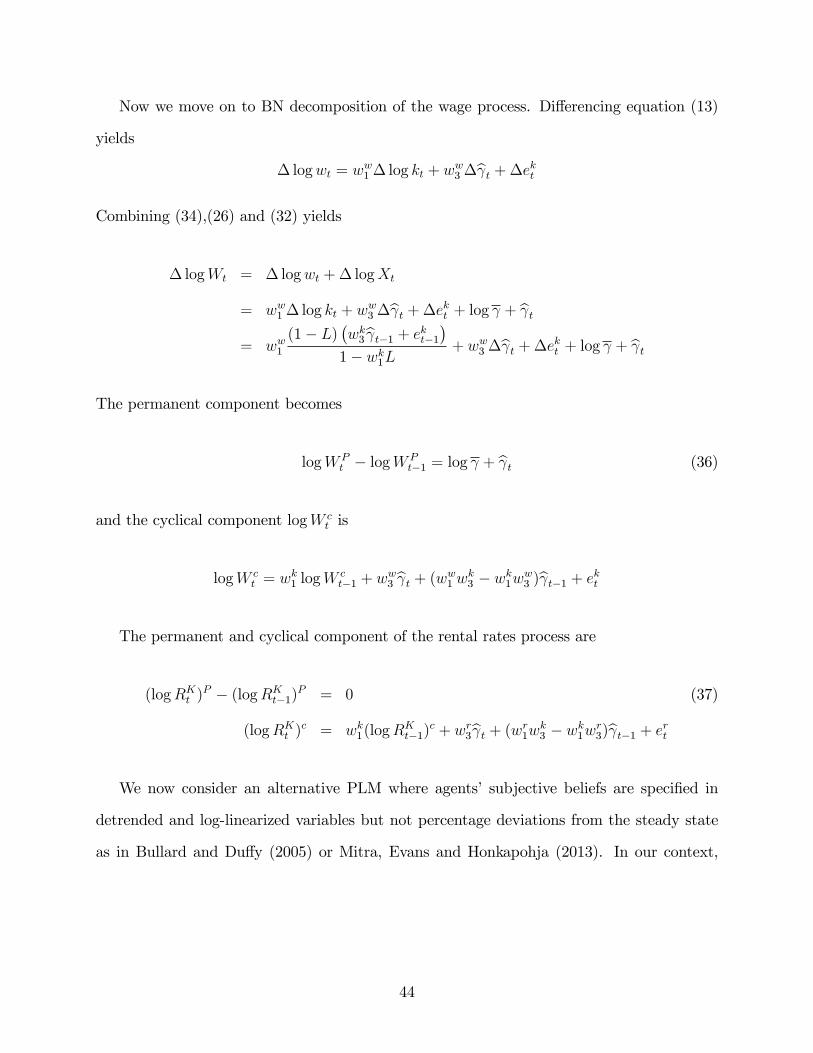
Now we move on to BN decomposition of the wage process. Differencing equation (13)
yields
∆ logwt = ww1 ∆ log kt + ww3 ∆γt + ∆ekt
Combining (34),(26) and (32) yields
∆ logWt = ∆ logwt + ∆ logXt
= ww1 ∆ log kt + ww3 ∆γt + ∆ekt + log γ + γt
= ww1(1− L)
(wk3 γt−1 + ekt−1
)1− wk1L
+ ww3 ∆γt + ∆ekt + log γ + γt
The permanent component becomes
logW Pt − logW P
t−1 = log γ + γt (36)
and the cyclical component logW ct is
logW ct = wk1 logW c
t−1 + ww3 γt + (ww1 wk3 − wk1ww3 )γt−1 + ekt
The permanent and cyclical component of the rental rates process are
(logRKt )P − (logRK
t−1)P = 0 (37)
(logRKt )c = wk1(logRK
t−1)c + wr3γt + (wr1wk3 − wk1wr3)γt−1 + ert
We now consider an alternative PLM where agents’ subjective beliefs are specified in
detrended and log-linearized variables but not percentage deviations from the steady state
as in Bullard and Duffy (2005) or Mitra, Evans and Honkapohja (2013). In our context,
44
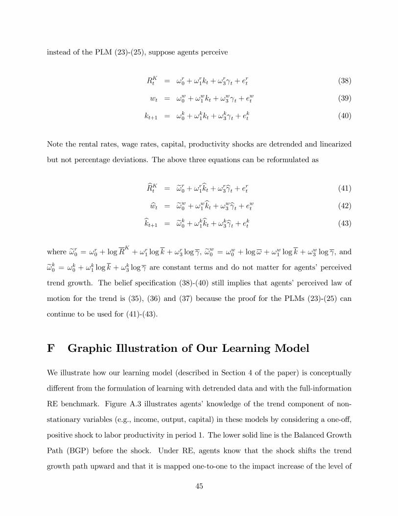
instead of the PLM (23)-(25), suppose agents perceive
RKt = ωr0 + ωr1kt + ωr3γt + ert (38)
wt = ωw0 + ωw1 kt + ωw3 γt + ewt (39)
kt+1 = ωk0 + ωk1kt + ωk3γt + ekt (40)
Note the rental rates, wage rates, capital, productivity shocks are detrended and linearized
but not percentage deviations. The above three equations can be reformulated as
RKt = ωr0 + ωr1kt + ωr3γt + ert (41)
wt = ωw0 + ωw1 kt + ωw3 γt + ewt (42)
kt+1 = ωk0 + ωk1kt + ωk3γt + ekt (43)
where ωr0 = ωr0 + logRK
+ ωr1 log k + ωr3 log γ, ωw0 = ωw0 + logω + ωw1 log k + ωw3 log γ, and
ωk0 = ωk0 + ωk1 log k + ωk3 log γ are constant terms and do not matter for agents’perceived
trend growth. The belief specification (38)-(40) still implies that agents’perceived law of
motion for the trend is (35), (36) and (37) because the proof for the PLMs (23)-(25) can
continue to be used for (41)-(43).
F Graphic Illustration of Our Learning Model
We illustrate how our learning model (described in Section 4 of the paper) is conceptually
different from the formulation of learning with detrended data and with the full-information
RE benchmark. Figure A.3 illustrates agents’knowledge of the trend component of non-
stationary variables (e.g., income, output, capital) in these models by considering a one-off,
positive shock to labor productivity in period 1. The lower solid line is the Balanced Growth
Path (BGP) before the shock. Under RE, agents know that the shock shifts the trend
growth path upward and that it is mapped one-to-one to the impact increase of the level of
45

the trend. In addition, agents know that the slope of the new BGP (i.e., the middle solid
line) is identical to that of the old path.
In the learning model where agents learn the law of motion for detrended variables, agents
too have exact knowledge that the shock is mapped one-to-one to the shift of the new trend
path and that the slope of the new BGP is not changed (as under RE). Unlike RE, however,
in this learning model agents do not know the location of the two BGPs and are uncertain
about the level of the trend component.
In our learning model, agents do not have exact knowledge of the new BGP relative to
the old one. They are uncertain about both the level and slope of the BGP after the shock.
The dotted solid line at the top in Figure A.3 represents the agents’ perceived path for
the trend after the shock in our learning model. As agents do statistical filtering, adding a
new observation to agents’information set changes the estimate of both the level and slope.
Thereafter, agents gradually revise their beliefs of the level and trend growth over time. To
reiterate, under RE or in models with learning detrending variables, agents know that the
long-run growth rates of non-stationary variables are identical to each other. In our model
agents can temporarily have the belief that the long-run growth rates of different variables
are not equal.
References for Online Appendix
Bullard, J., and J., Duffy (2005). Learning and Structural Change in Macroeconomic
Data. Federal Reserve Bank of St. Louis Working Paper 2004-016A.
Cogley T., and Sargent (2008), Anticipated Utility and Rational Expectations as Ap-
proximations of Bayesian Decision Making. International Economic Review 49, 185-221.
Eusepi, S., and B., Preston (2011). Expectations, Learning and Business Cycle Fluctua-
tions. American Economic Review 101(6): 2844-72.
Evans, G., S., Honkapohja and N., Williams (2005). Generalized Stochastic Gradient
Learning. NBER technical working paper 317.
46
Evans, G., S., Honkapohja, and N., Williams (2010). Generalized Stochastic Gradient
Learning. International Economic Review 51, 237-262.
Favero, C., (2001). Applied Macroeconometrics. Oxford University Press.
Granger, C.W.J., and P. Newbold, (1986). Forecasting Economic Time Series, 3rd ed.
Orlando, FL: Academic Press.
Kreps, D. M., (1998). Anticipated Utility and Dynamic Choice. In Frontiers of Research
in Economic Theory, pp. 242– 274. Jacobs, D., E. Kalai, and M. Kamien (eds.). Cambridge
University Press, Cambridge.
Mitra, K., G., Evans, and S., Honkapohja, (2013). Policy Change and Learning in the
Real Business Cycle Model. Journal of Economic Dynamics and Control 37, 1947-1971.
47
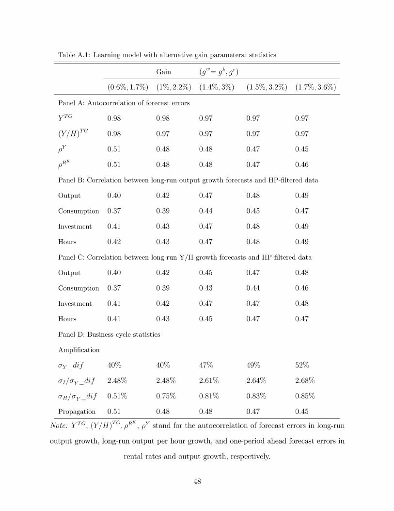
Table A.1: Learning model with alternative gain parameters: statistics
Gain (gw= gk, gr)
(0.6%, 1.7%) (1%, 2.2%) (1.4%, 3%) (1.5%, 3.2%) (1.7%, 3.6%)
Panel A: Autocorrelation of forecast errors
Y TG 0.98 0.98 0.97 0.97 0.97
(Y/H)TG 0.98 0.97 0.97 0.97 0.97
ρY 0.51 0.48 0.48 0.47 0.45
ρRK
0.51 0.48 0.48 0.47 0.46
Panel B: Correlation between long-run output growth forecasts and HP-filtered data
Output 0.40 0.42 0.47 0.48 0.49
Consumption 0.37 0.39 0.44 0.45 0.47
Investment 0.41 0.43 0.47 0.48 0.49
Hours 0.42 0.43 0.47 0.48 0.49
Panel C: Correlation between long-run Y/H growth forecasts and HP-filtered data
Output 0.40 0.42 0.45 0.47 0.48
Consumption 0.37 0.39 0.43 0.44 0.46
Investment 0.41 0.42 0.47 0.47 0.48
Hours 0.41 0.43 0.45 0.47 0.47
Panel D: Business cycle statistics
Amplification
σY_dif 40% 40% 47% 49% 52%
σI/σY_dif 2.48% 2.48% 2.61% 2.64% 2.68%
σH/σY_dif 0.51% 0.75% 0.81% 0.83% 0.85%
Propagation 0.51 0.48 0.48 0.47 0.45
Note: Y TG, (Y/H)TG, ρRK, ρY stand for the autocorrelation of forecast errors in long-run
output growth, long-run output per hour growth, and one-period ahead forecast errors in
rental rates and output growth, respectively.
48
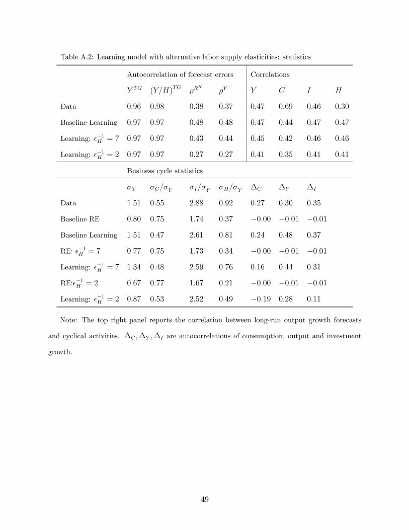
Table A.2: Learning model with alternative labor supply elasticities: statistics
Autocorrelation of forecast errors Correlations
Y TG (Y/H)TG ρRK
ρY Y C I H
Data 0.96 0.98 0.38 0.37 0.47 0.69 0.46 0.30
Baseline Learning 0.97 0.97 0.48 0.48 0.47 0.44 0.47 0.47
Learning: ε−1H = 7 0.97 0.97 0.43 0.44 0.45 0.42 0.46 0.46
Learning: ε−1H = 2 0.97 0.97 0.27 0.27 0.41 0.35 0.41 0.41
Business cycle statistics
σY σC/σY σI/σY σH/σY ∆C ∆Y ∆I
Data 1.51 0.55 2.88 0.92 0.27 0.30 0.35
Baseline RE 0.80 0.75 1.74 0.37 −0.00 −0.01 −0.01
Baseline Learning 1.51 0.47 2.61 0.81 0.24 0.48 0.37
RE: ε−1H = 7 0.77 0.75 1.73 0.34 −0.00 −0.01 −0.01
Learning: ε−1H = 7 1.34 0.48 2.59 0.76 0.16 0.44 0.31
RE:ε−1H = 2 0.67 0.77 1.67 0.21 −0.00 −0.01 −0.01
Learning: ε−1H = 2 0.87 0.53 2.52 0.49 −0.19 0.28 0.11
Note: The top right panel reports the correlation between long-run output growth forecasts
and cyclical activities. ∆C ,∆Y ,∆I are autocorrelations of consumption, output and investment
growth.
49
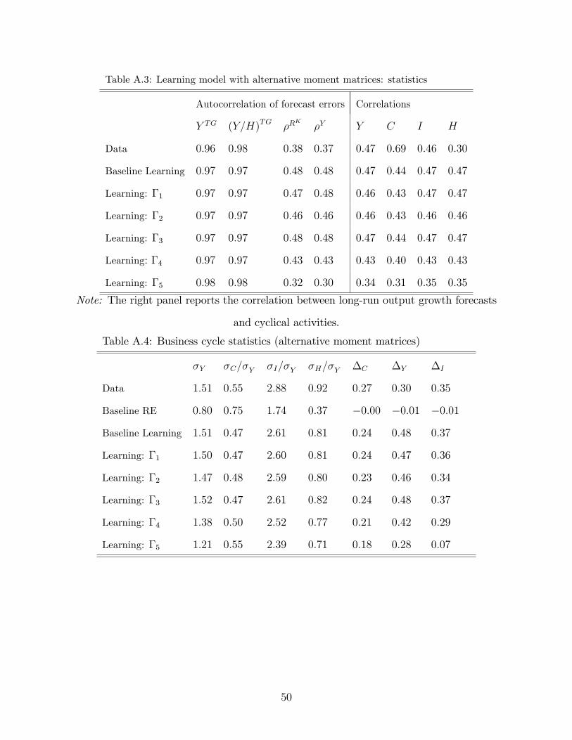
Table A.3: Learning model with alternative moment matrices: statistics
Autocorrelation of forecast errors Correlations
Y TG (Y/H)TG ρRK
ρY Y C I H
Data 0.96 0.98 0.38 0.37 0.47 0.69 0.46 0.30
Baseline Learning 0.97 0.97 0.48 0.48 0.47 0.44 0.47 0.47
Learning: Γ1 0.97 0.97 0.47 0.48 0.46 0.43 0.47 0.47
Learning: Γ2 0.97 0.97 0.46 0.46 0.46 0.43 0.46 0.46
Learning: Γ3 0.97 0.97 0.48 0.48 0.47 0.44 0.47 0.47
Learning: Γ4 0.97 0.97 0.43 0.43 0.43 0.40 0.43 0.43
Learning: Γ5 0.98 0.98 0.32 0.30 0.34 0.31 0.35 0.35
Note: The right panel reports the correlation between long-run output growth forecasts
and cyclical activities.
Table A.4: Business cycle statistics (alternative moment matrices)
σY σC/σY σI/σY σH/σY ∆C ∆Y ∆I
Data 1.51 0.55 2.88 0.92 0.27 0.30 0.35
Baseline RE 0.80 0.75 1.74 0.37 −0.00 −0.01 −0.01
Baseline Learning 1.51 0.47 2.61 0.81 0.24 0.48 0.37
Learning: Γ1 1.50 0.47 2.60 0.81 0.24 0.47 0.36
Learning: Γ2 1.47 0.48 2.59 0.80 0.23 0.46 0.34
Learning: Γ3 1.52 0.47 2.61 0.82 0.24 0.48 0.37
Learning: Γ4 1.38 0.50 2.52 0.77 0.21 0.42 0.29
Learning: Γ5 1.21 0.55 2.39 0.71 0.18 0.28 0.07
50
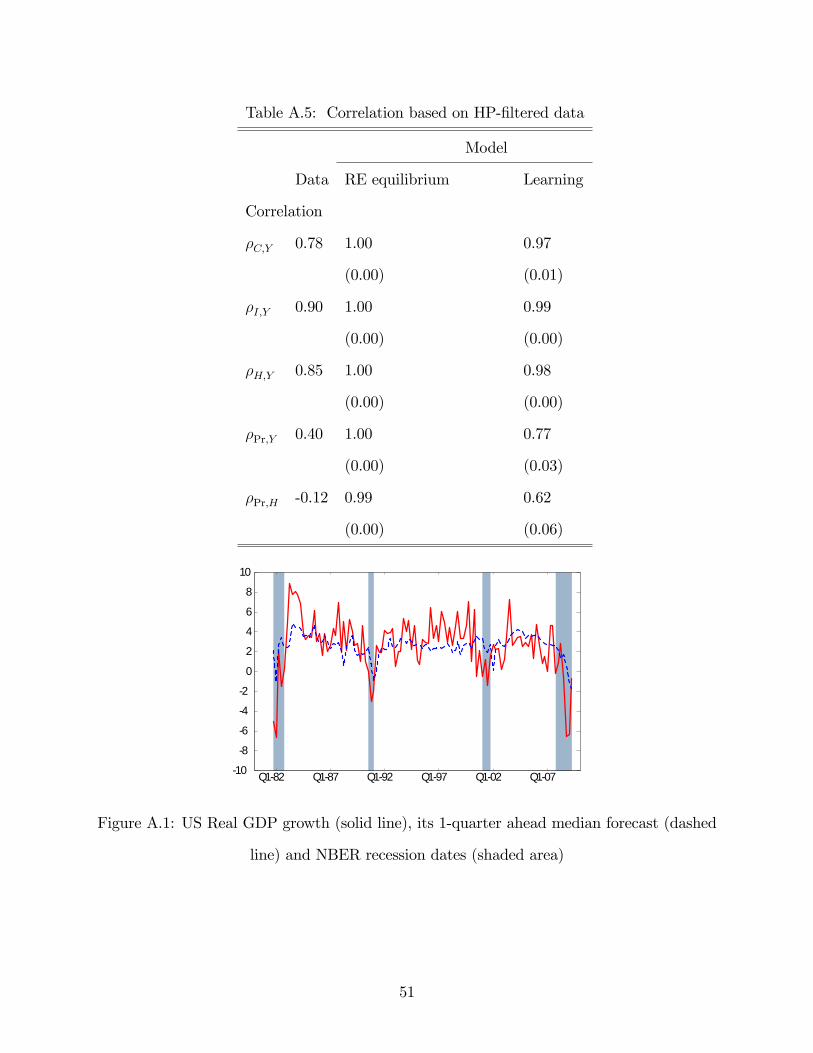
Table A.5: Correlation based on HP-filtered data
Model
Data RE equilibrium Learning
Correlation
ρC,Y 0.78 1.00 0.97
(0.00) (0.01)
ρI,Y 0.90 1.00 0.99
(0.00) (0.00)
ρH,Y 0.85 1.00 0.98
(0.00) (0.00)
ρPr,Y 0.40 1.00 0.77
(0.00) (0.03)
ρPr,H -0.12 0.99 0.62
(0.00) (0.06)
Q182 Q187 Q192 Q197 Q102 Q10710
8
6
4
2
0
2
4
6
8
10
Figure A.1: US Real GDP growth (solid line), its 1-quarter ahead median forecast (dashed
line) and NBER recession dates (shaded area)
51

0 20 401
2
3
% d
ev. f
rom
uns
hock
ed B
GP
Output
RELearning
0 20 400
5
10Investment
0 20 400.5
1
1.5Consumption
0 20 400
1
2Hours
0 20 402.1
2.15
2.2LR Y Growth forecast
Ann
ualiz
ed %
0 20 402.1
2.15
2.2LR Y/H growth forecast
Ann
ualiz
ed %
Figure A.2: Impulse response to a 1% positive productivity shock under CG-RLS learning
1Time
RE and Learning Detrended Variables
Our M odel
Figure A.3: Agents’Perceived Law of Motion for the Trend
52
Recommended


