Bayesian machine learning: a tutorial
Remi Bardenet
CNRS & CRIStAL, Univ. Lille, France
Remi Bardenet (CNRS & Univ. Lille) Bayesian ML 1

OutlineThe what
Typical statistical problemsStatistical decision theoryPosterior expected utility and Bayes rules
The whyThe philosophical whyThe practical why
The howConjugacyMonte Carlo methodsMetropolis-HastingsVariational approximations
In depth with Gaussian processes in MLFrom linear regression to GPsModeling and learningMore applicationsReferences and open issues
Remi Bardenet (CNRS & Univ. Lille) Bayesian ML 2

OutlineThe what
Typical statistical problemsStatistical decision theoryPosterior expected utility and Bayes rules
The whyThe philosophical whyThe practical why
The howConjugacyMonte Carlo methodsMetropolis-HastingsVariational approximations
In depth with Gaussian processes in MLFrom linear regression to GPsModeling and learningMore applicationsReferences and open issues
Remi Bardenet (CNRS & Univ. Lille) Bayesian ML 3

Typical jobs for statisticians
Estimation
I You have data x1, . . . , xn that you assume drawn fromp(x1, . . . , xn|θ?), with θ? ∈ Rd .
I You want an estimate θ(x1, . . . , xn) of θ? ∈ Rd .
Confidence regions
I You have data x1, . . . , xn that you assume drawn fromp(x1, . . . , xn · |θ?), with θ? ∈ Rd .
I You want a region A(x1, . . . , xn) ⊂ Rd and make a statementthat θ ∈ A(x1, . . . , xn) with some certainty.
Remi Bardenet (CNRS & Univ. Lille) Bayesian ML 4
Statistical decision theory1
Figure: Abraham Wald (1902–1950)
1A. Wald. Statistical decision functions. Wiley, 1950.Remi Bardenet (CNRS & Univ. Lille) Bayesian ML 5

Statistical decision theory
I Let Θ be the “states of the world”, typically the space ofparameters of interest.
I Decisions are functions d(x1, . . . , xn) ∈ D.
I Let L(d , θ) denote the loss of making decision d when thestate of the world is θ.
I Wald defines the risk of a decision as
R(d , θ) =
∫L(d , θ)p(x1:n|θ)dx1:n.
I Wald says d1 is a better decision than d2 if
∀θ ∈ Θ, L(d1, θ) 6 L(d2, θ). (1)
I d is called admissible if there is no better decision than d .
Remi Bardenet (CNRS & Univ. Lille) Bayesian ML 6

Illustration with a simple estimation problem
I You have data x1, . . . , xn that you assume drawn from
p(x1, . . . , xn|θ?) =n∏
i=1
N (xi |θ?, σ2),
and you know σ2.
I You choose a loss function, say L(θ, θ) = ‖θ − θ‖2.
I You restrict your decision space to unbiased estimators.
I The sample mean θ := n−1∑n
i=1 xi is unbiased, and hasminimum variance among unbiased estimators.
I SinceR(θ, θ) = Varθ,
θ is the best decision you can make in Wald’s framework.
Remi Bardenet (CNRS & Univ. Lille) Bayesian ML 7

Wald’s view of frequentist estimation
Estimation
I You have data x1, . . . , xn that you assume drawn fromp(x1, . . . , xn|θ?), with θ? ∈ Rd .
I You want an estimate θ(x1, . . . , xn) of θ? ∈ Rd .
A Waldian answer
I Our decisions are estimates d(x1, . . . , xn) = θ(x1, . . . , xn).
I We pick a loss, say L(d , θ) = L(θ, θ) = ‖θ − θ‖2.
I If you have an unbiased estimator with minimum variance,then this is the best decision among unbiased estimators.
Remi Bardenet (CNRS & Univ. Lille) Bayesian ML 8

Wald’s view of frequentist estimation
Estimation
I You have data x1, . . . , xn that you assume drawn fromp(x1, . . . , xn|θ?), with θ? ∈ Rd .
I You want an estimate θ(x1, . . . , xn) of θ? ∈ Rd .
A Waldian answer
I Our decisions are estimates d(x1, . . . , xn) = θ(x1, . . . , xn).
I In general, the loss can be more complex and unbiasedestimors unknown/irrelevant.
I In these cases, you may settle for a minimax estimator
θ(x1, . . . , xn) = arg mind
supθ
R(d , θ).
Remi Bardenet (CNRS & Univ. Lille) Bayesian ML 8

Wald’s is only one view of frequentist statistics...
I On estimation, some would argue in favour of the maximumlikelihood2.
Figure: Ronald Fisher (1890–1962)
2S. M. Stigler. “The epic story of maximum likelihood”. In: StatisticalScience (2007), pp. 598–620.
Remi Bardenet (CNRS & Univ. Lille) Bayesian ML 9

... but bear with me, since it is predominant in machine learning
For instance, supervised learning is usually formalized as
g? = arg ming
EL(y , g(x)). (2)
which you approximate by
g = arg ming
n∑i=1
L(yi , g(xi )) + penalty(g),
while trying to control the excess risk
EL(y , g(x))− EL(y , g?(x)).
Remi Bardenet (CNRS & Univ. Lille) Bayesian ML 10

Wald’s view of frequentist confidence regions
Confidence regions
I You have data x1, . . . , xn that you assume drawn fromp(x1, . . . , xn · |θ?), with θ? ∈ Rd .
I You want a region A(x1, . . . , xn) ⊂ Rd and make a statementthat θ ∈ A(x1, . . . , xn) with some certainty.
A Waldian answer
I Our decisions are subsets of Rd : d(x1:n) = A(x1:n).
I A common loss is L(d , θ) = L(A, θ) = 1θ/∈A + γ|A|.I So you want to find A(x1:n) that minimizes
L(A, θ) =
∫[1θ? /∈Ap(x1:n|θ?) + γ|A|] dx1:n.
Remi Bardenet (CNRS & Univ. Lille) Bayesian ML 11

Illustration with a simple confidence interval problem
I You have data x1, . . . , xn that you assume drawn from
p(x1, . . . , xn|θ?) =n∏
i=1
N (xi |θ?, σ2).
I You choose a loss function, say L(A, θ) = 1θ/∈A + γ|A|.I You restrict your decisions to intervals centered around the
sample mean θ.
I Since θ−θσ/√n∼ N (0, 1), we know (exercise) that for
A := [θ − kσ/√n, θ + kσ/
√n],
it comes
R(A, θ) = P(|N (0, 1)| > k) +2γkσ√
n.
I All is left to do is choose k .I Textbook examples bypass the need for γ: they fix α > 0 and
find the smallest k such that P(|N (0, 1)| > k) 6 α.
Remi Bardenet (CNRS & Univ. Lille) Bayesian ML 12

Summary so far
I Waldian frequentists measure risks as expectations w.r.t. thedata-generating process.
R(d , θ) =
∫L(d(x1:n), θ)p(x1:n|θ)dx1:n
I One major difficulty is that the risk remains a function of θ.
I Without additional structure (unbiasedness, Gaussianity, etc.),it is difficult to go beyond minimax rules.
Idea
What if we introduced a distribution on Θ, and tried to minimize
r(d) =
∫R(d , θ)p(θ)dθ
=
∫ [∫L(d(x1:n), θ)p(x1:n|θ)dx1:n
]p(θ)dθ
Remi Bardenet (CNRS & Univ. Lille) Bayesian ML 13

From expected frequentist loss to posterior expected loss
r(d) =
∫R(d , θ)p(θ)dθ
=
∫ [∫L(d(x1:n), θ)p(x1:n|θ)dx1:n
]p(θ)dθ
=
∫ [∫L(d(x1:n), θ)p(x1:n|θ)p(θ)dθ
]dx1:n
=
∫ [∫L(d(x1:n), θ)
p(x1:n|θ)p(θ)
p(x1:n)dθ
]p(x1:n)dx1:n
=
∫ [∫L(d(x1:n), θ)p(θ|x1:n)dθ
]p(x1:n)dx1:n
Remi Bardenet (CNRS & Univ. Lille) Bayesian ML 14

Bayesians minimize posterior expected utility
The posterior expected utility paradigm: Bayes rules
Pick d to solve
arg mind
∫L(d(x1:n), θ)p(θ|x1:n)dθ.
Bayes rules have good frequentist properties3
I Under general conditions, Bayes decision rules are admissible,all admissible rules are limits of Bayes rules.
I Bayes rules with “least favourable priors” are minimax.
3G. Parmigiani and L. Inoue. Decision theory: principles and approaches.Vol. 812. John Wiley & Sons, 2009.
Remi Bardenet (CNRS & Univ. Lille) Bayesian ML 15

Illustration with a simple estimation problem
I You have data x1, . . . , xn that you assume drawn from
p(x1, . . . , xn|θ?) =n∏
i=1
N (xi |θ?, σ2),
and you know σ2.
I You choose a loss function, say L(θ, θ) = ‖θ − θ‖2.
I You choose a prior p over θ.
I Your Bayes decision minimizes∫‖θ − θ‖2p(θ|x1:n)dθ,
so you pick
θ =
∫θp(θ|x1:n)dθ.
I Conceptually, it is simpler. In practice, you need to computean integral.
Remi Bardenet (CNRS & Univ. Lille) Bayesian ML 16

Illustration with a simple confidence interval problem
I You have data x1, . . . , xn that you assume drawn from
p(x1, . . . , xn|θ?) =n∏
i=1
N (xi |θ?, σ2).
I You choose a loss function, say L(A, θ) = 1θ/∈A + γ|A|.I You choose a prior p over θ.
I Your Bayes decision minimizes∫1θ/∈Ap(θ|x1:n)dθ + γ|A|,
I Conceptually, it is simpler. In practice, you need to carefullypick your prior and/or restrict the decision space and/orcompute many integrals.
Remi Bardenet (CNRS & Univ. Lille) Bayesian ML 17

Summary so far
I Bayes rules fit into Wald’s framework.
I For a fixed prior, the Bayesian risk completely orders decisionrules.
I The key idea is posterior expected utility.
I You can answer most basic statistical questions using thisprinciple: [more examples].
Remi Bardenet (CNRS & Univ. Lille) Bayesian ML 18

A recent motivating success
GW170814: A Three-Detector Observation of Gravitational Wavesfrom a Binary Black Hole Coalescence
B. P. Abbott et al.*
(LIGO Scientific Collaboration and Virgo Collaboration)(Received 23 September 2017; published 6 October 2017)
On August 14, 2017 at 10∶30:43 UTC, the Advanced Virgo detector and the two Advanced LIGOdetectors coherently observed a transient gravitational-wave signal produced by the coalescence of twostellar mass black holes, with a false-alarm rate of ≲1 in 27 000 years. The signal was observed with athree-detector network matched-filter signal-to-noise ratio of 18. The inferred masses of the initial blackholes are 30.5þ5.7
−3.0M⊙ and 25:3þ2.8−4.2M⊙ (at the 90% credible level). The luminosity distance of the source is
540þ130−210 Mpc, corresponding to a redshift of z ¼ 0.11þ0.03
−0.04 . A network of three detectors improves the skylocalization of the source, reducing the area of the 90% credible region from 1160 deg2 using only the twoLIGO detectors to 60 deg2 using all three detectors. For the first time, we can test the nature ofgravitational-wave polarizations from the antenna response of the LIGO-Virgo network, thus enabling anew class of phenomenological tests of gravity.
DOI: 10.1103/PhysRevLett.119.141101
I. INTRODUCTION
The era of gravitational-wave (GW) astronomy beganwith the detection of binary black hole (BBH) mergers, bythe Advanced Laser Interferometer Gravitational-WaveObservatory (LIGO) detectors [1], during the first of theAdvanced Detector Observation Runs. Three detections,GW150914 [2], GW151226 [3], and GW170104 [4], and alower significance candidate, LVT151012 [5], have beenannounced so far. The Advanced Virgo detector [6] joinedthe second observation run on August 1, 2017.On August 14, 2017, GWs from the coalescence of two
black holes at a luminosity distance of 540þ130−210 Mpc, with
masses of 30.5þ5.7−3.0M⊙ and 25.3þ2.8
−4.2M⊙, were observed in allthree detectors. The signal was first observed at the LIGOLivingston detector at 10∶30:43 UTC, and at the LIGOHanford and Virgo detectors with a delay of ∼8 ms and∼14 ms, respectively.The signal-to-noise ratio (SNR) time series, the time-
frequency representation of the strain data, and the timeseries data of the three detectors together with the inferredGW waveform, are shown in Fig. 1. The different sensitiv-ities and responses of the three detectors result in the GWproducing different values of matched-filter SNR in eachdetector.Three methods were used to assess the impact of the
Virgo instrument on this detection. (a) Using the best fit
waveform obtained from analysis of the LIGO detectors’data alone, we find that the probability, in 5000 s of dataaround the event, of a peak in SNR from Virgo data due tonoise and as large as the one observed, within a timewindow determined by the maximum possible time offlight, is 0.3%. (b) A search for unmodeled GW transientsdemonstrates that adding Advanced Virgo improves thefalse-alarm rate by an order of magnitude over thetwo-detector network. (c) We compare the matched-filtermarginal likelihood for a model with a coherent BBHsignal in all three detectors to that for a model assumingpure Gaussian noise in Virgo and a BBH signal only in theLIGO detectors: the three detector BBH signal model ispreferred with a Bayes factor of more than 1600.Until Advanced Virgo became operational, typical GW
position estimates were highly uncertain compared to thefields of view of most telescopes. The baseline formed bythe two LIGO detectors allowed us to localize most mergersto roughly annular regions spanning hundreds to about athousand square degrees at the 90% credible level [7–9].Virgo adds additional independent baselines, which incases such as GW170814 can reduce the positionaluncertainty by an order of magnitude or more [8].Tests of general relativity (GR) in the strong field regime
have been performed with the signals from the BBHmergers detected by the LIGO interferometers [2–5,10].In GR, GWs are characterized by two tensor (spin-2)polarizations only, whereas generic metric theories mayallow up to six polarizations [11,12]. As the two LIGOinstruments have similar orientations, little informationabout polarizations can be obtained using the LIGOdetectors alone. With the addition of Advanced Virgowe can probe, for the first time, gravitational-wave polar-izations geometrically by projecting the wave’s amplitude
*Full author list given at the end of the Letter.
Published by the American Physical Society under the terms ofthe Creative Commons Attribution 4.0 International license.Further distribution of this work must maintain attribution tothe author(s) and the published article’s title, journal citation,and DOI.
PRL 119, 141101 (2017) P HY S I CA L R EV I EW LE T T ER Sweek ending
6 OCTOBER 2017
0031-9007=17=119(14)=141101(16) 141101-1 Published by the American Physical Society
Remi Bardenet (CNRS & Univ. Lille) Bayesian ML 19

OutlineThe what
Typical statistical problemsStatistical decision theoryPosterior expected utility and Bayes rules
The whyThe philosophical whyThe practical why
The howConjugacyMonte Carlo methodsMetropolis-HastingsVariational approximations
In depth with Gaussian processes in MLFrom linear regression to GPsModeling and learningMore applicationsReferences and open issues
Remi Bardenet (CNRS & Univ. Lille) Bayesian ML 20
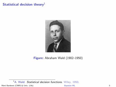
The subjectivistic viewpoint
I Top requirement is internal coherence of decisions.
I Favourizes interpreting probability distributions as personalbeliefs.
Figure: Bruno de Finetti (1906–1985) and L. Jimmie Savage(1917–1971)
Remi Bardenet (CNRS & Univ. Lille) Bayesian ML 21

The logical justification
I Top requirement is to find a version of propositional logic thatallows taking into account uncertainty.
I Also favourizes interpreting probability distributions as beliefs,but aims for objective priors.
Figure: Richart T. Cox (1898–1991), Edwin T. Jaynes(1917–1971), and Harold Jeffreys (1891–1989)
Remi Bardenet (CNRS & Univ. Lille) Bayesian ML 22

The hybrid view4
I The starting point is posterior expected utility, loosely justifiedby Wald’s theory.
I It is simple, widely applicable, has good frequentist properties.
I It satisfies the likelihood principle.I It is easy to interpret: beliefs are
I represented by probabilities,I updated using Bayes’ rule,I integrated when making decisions.
I It is easy to communicate your uncertaintyI Simply give your posterior.I When making a decision, make sure that the priors of everyone
involved would yield the same decision.
4C. P. Robert. The Bayesian choice: from decision-theoretic foundations tocomputational implementation. Springer Science & Business Media, 2007.
Remi Bardenet (CNRS & Univ. Lille) Bayesian ML 23

Practical advantages of posterior expected utility
I Conceptually answers all ML problems.
I Suits all applications where quantifying uncertainty is vital vscomputational complexity: all basic sciences, health, evenone-shot commercial decisions.
I We never invoked any large-sample argument, so suits all sizesof datasets.
Remi Bardenet (CNRS & Univ. Lille) Bayesian ML 24

OutlineThe what
Typical statistical problemsStatistical decision theoryPosterior expected utility and Bayes rules
The whyThe philosophical whyThe practical why
The howConjugacyMonte Carlo methodsMetropolis-HastingsVariational approximations
In depth with Gaussian processes in MLFrom linear regression to GPsModeling and learningMore applicationsReferences and open issues
Remi Bardenet (CNRS & Univ. Lille) Bayesian ML 25

Conjugacy
I Say we have a linear regression problem
yi = f (xi ) + εi ,
f (x) = θT x , εi i.i.d. Gaussians N (0, σ2).
I If we choose p(θ) ∼ N (0,Σ), then (exercise)
p(θ|(x , y)1:n) ∝ p((x , y)1:n|θ)p(θ)
= N (σ−2A−1Xy,A−1),
where A = σ−2XTX + Σ−1.
I If the loss is not too complicated, then integrals are easy. Forinstance, prediction with L2 loss is simple:
Remi Bardenet (CNRS & Univ. Lille) Bayesian ML 26

Conjugacy
I Say we have a linear regression problem
yi = f (xi ) + εi ,
f (x) = θT x , εi i.i.d. Gaussians N (0, σ2).
I If we choose p(θ) ∼ N (0,Σ), then (exercise)
p(θ|(x , y)1:n) ∝ p((x , y)1:n|θ)p(θ)
= N (σ−2A−1Xy,A−1),
where A = σ−2XTX + Σ−1.
I If the loss is not too complicated, then integrals are easy. Forinstance, prediction with L2 loss is simple:
arg miny?
∫‖y? − f (x?)‖2p(θ|(x , y)1:n)dθ
Remi Bardenet (CNRS & Univ. Lille) Bayesian ML 26

Conjugacy
I Say we have a linear regression problem
yi = f (xi ) + εi ,
f (x) = θT x , εi i.i.d. Gaussians N (0, σ2).
I If we choose p(θ) ∼ N (0,Σ), then (exercise)
p(θ|(x , y)1:n) ∝ p((x , y)1:n|θ)p(θ)
= N (σ−2A−1Xy,A−1),
where A = σ−2XTX + Σ−1.
I If the loss is not too complicated, then integrals are easy. Forinstance, prediction with L2 loss is simple:
arg miny?
∫‖y? − θT x?‖2p(θ|(x , y)1:n)dθ
Remi Bardenet (CNRS & Univ. Lille) Bayesian ML 26

Conjugacy
I Say we have a linear regression problem
yi = f (xi ) + εi ,
f (x) = θT x , εi i.i.d. Gaussians N (0, σ2).
I If we choose p(θ) ∼ N (0,Σ), then (exercise)
p(θ|(x , y)1:n) ∝ p((x , y)1:n|θ)p(θ)
= N (σ−2A−1Xy,A−1),
where A = σ−2XTX + Σ−1.
I If the loss is not too complicated, then integrals are easy. Forinstance, prediction with L2 loss is simple:
y? := σ−2xT? A−1Xy.
Remi Bardenet (CNRS & Univ. Lille) Bayesian ML 26

Monte Carlo methods
I Sometimes, you’re less lucky. Say we’re doing logisticregression.
yi = Bernoulli [σ(f (xi ))] ,
with f (x) = θT x , σ(x) = 1/(1 + e−x).
I Even if we choose p(θ) ∼ N (0,Σ),
p(θ|(x , y)1:n) ∝ p((x , y)1:n|θ)p(θ)
does not have a simple closed form.
I We need powerful numerical integration methods, that is,constructions of nodes (θi ) and weights wi such that∫
hdπ ≈N∑i=1
wih(θi ).
Remi Bardenet (CNRS & Univ. Lille) Bayesian ML 27

Metropolis-Hastings
MH(π(θ), q(θ′|θ), θ0, Niter
)1 for k ← 1 to Niter
2 θ ← θk−1
3 θ′ ∼ q(.|θ), u ∼ U(0,1),
4 α = π(θ′)π(θ)
q(θ|θ′)q(θ′|θ)
5 if u < α
6 θk ← θ′ . Accept
7 else θk ← θ . Reject
8 return (θk)k=1,...,Niter
Remi Bardenet (CNRS & Univ. Lille) Bayesian ML 28

Metropolis-Hastings
MH(π(θ), q(θ′|θ), θ0, Niter
)1 for k ← 1 to Niter
2 θ ← θk−1
3 θ′ ∼ q(.|θ), u ∼ U(0,1),
4 α = π(θ′)π(θ)
q(θ|θ′)q(θ′|θ)
5 if u < α
6 θk ← θ′ . Accept
7 else θk ← θ . Reject
8 return (θk)k=1,...,Niter
Remi Bardenet (CNRS & Univ. Lille) Bayesian ML 28

Metropolis-Hastings
MH(π(θ), q(θ′|θ), θ0, Niter
)1 for k ← 1 to Niter
2 θ ← θk−1
3 θ′ ∼ q(.|θ), u ∼ U(0,1),
4 α = π(θ′)π(θ)
q(θ|θ′)q(θ′|θ)
5 if u < α
6 θk ← θ′ . Accept
7 else θk ← θ . Reject
8 return (θk)k=1,...,Niter
Remi Bardenet (CNRS & Univ. Lille) Bayesian ML 28

Metropolis-Hastings
MH(π(θ), q(θ′|θ), θ0, Niter
)1 for k ← 1 to Niter
2 θ ← θk−1
3 θ′ ∼ q(.|θ), u ∼ U(0,1),
4 α = π(θ′)π(θ)
q(θ|θ′)q(θ′|θ)
5 if u < α
6 θk ← θ′ . Accept
7 else θk ← θ . Reject
8 return (θk)k=1,...,Niter
Remi Bardenet (CNRS & Univ. Lille) Bayesian ML 28

Metropolis-Hastings
MH(π(θ), q(θ′|θ), θ0, Niter
)1 for k ← 1 to Niter
2 θ ← θk−1
3 θ′ ∼ q(.|θ), u ∼ U(0,1),
4 α = π(θ′)π(θ)
q(θ|θ′)q(θ′|θ)
5 if u < α
6 θk ← θ′ . Accept
7 else θk ← θ . Reject
8 return (θk)k=1,...,Niter
Remi Bardenet (CNRS & Univ. Lille) Bayesian ML 28

The MCMC magic
I Under assumptions5,
√Niter
[1
Niter
Niter∑k=0
h(θk)−∫
h (θ)π(θ)dθ
]→ N (0, σ2
lim(h)),
I If you choose q carefully, you can hope for a polynomialincrease of the mixing time and σ2
lim(h) with d .
I Most MCMC algorithms are instances of Metropolis-Hastingswith clever choices of proposal6, even the NUTS HMC of Stanand PyMC3.
I For nice illustrations, check outhttps://chi-feng.github.io/mcmc-demo/
5R. Douc et al. Nonlinear time series. Chapman-Hall, 2014.6C. P. Robert and G. Casella. Monte Carlo Statistical Methods. New York:
Springer-Verlag, 2004.Remi Bardenet (CNRS & Univ. Lille) Bayesian ML 29

Variational approximations
I When in a hurry, you can settle for a good approximation toyour posterior
π(θ) = p(θ|x) ∝ p(x|θ)p(θ),
say minimize in q
KL(q, π) = Eq log q − Eq log p(θ|x)
= −[−Eq log q + Eq log p(x, θ)] + log p(x).
I Equivalently, we can maximize the evidence lower bound(ELBO)7.
I Ideally, I would rather cast the choice of q into a Wald-likeproblem.
7D. M. Blei et al. “Variational inference: A review for statisticians”. In:Journal of the American Statistical Association 112.518 (2017), pp. 859–877.
Remi Bardenet (CNRS & Univ. Lille) Bayesian ML 30

OutlineThe what
Typical statistical problemsStatistical decision theoryPosterior expected utility and Bayes rules
The whyThe philosophical whyThe practical why
The howConjugacyMonte Carlo methodsMetropolis-HastingsVariational approximations
In depth with Gaussian processes in MLFrom linear regression to GPsModeling and learningMore applicationsReferences and open issues
Remi Bardenet (CNRS & Univ. Lille) Bayesian ML 31

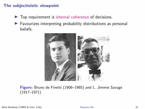
Linear regression
I yi = f (xi ) + εi , f (x) = θT x , εi i.i.d. Gaussians N (0, σ2).
I If we choose p(θ) ∼ N (0,Σ2), then
p(θ|(x , y)1:n) ∝ p((x , y)1:n|θ)p(θ)
= [Exercise]
where A = σ−2XTX + Σ−1.
Remi Bardenet (CNRS & Univ. Lille) Bayesian ML 32

Linear regression
I yi = f (xi ) + εi , f (x) = θT x , εi i.i.d. Gaussians N (0, σ2).
I If we choose p(θ) ∼ N (0,Σ2), then
p(θ|(x , y)1:n) ∝ p((x , y)1:n|θ)p(θ)
∝ exp
[−‖y − Xθ‖2
2σ2− θTΣ−1θ
2
]
where A = σ−2XTX + Σ−1.
Remi Bardenet (CNRS & Univ. Lille) Bayesian ML 32

Linear regression
I yi = f (xi ) + εi , f (x) = θT x , εi i.i.d. Gaussians N (0, σ2).
I If we choose p(θ) ∼ N (0,Σ2), then
p(θ|(x , y)1:n) ∝ p((x , y)1:n|θ)p(θ)
∝ exp
[−‖y − Xθ‖2
2σ2− θTΣ−1θ
2
]∝ exp
[yTXθ
σ2− θTXTXθ
2σ2− θTΣ−1θ
2
]∝ exp
[−1
2
(θ − σ−2A−1Xy
)TA(θ − σ−2A−1Xy
)]
where A = σ−2XTX + Σ−1.
Remi Bardenet (CNRS & Univ. Lille) Bayesian ML 32

Linear regression
I yi = f (xi ) + εi , f (x) = θT x , εi i.i.d. Gaussians N (0, σ2).
I If we choose p(θ) ∼ N (0,Σ2), then
p(θ|(x , y)1:n) ∝ p((x , y)1:n|θ)p(θ)
∝ exp
[−‖y − Xθ‖2
2σ2− θTΣ−1θ
2
]∝ exp
[yTXθ
σ2− θTXTXθ
2σ2− θTΣ−1θ
2
]∝ exp
[−1
2
(θ − σ−2A−1Xy
)TA(θ − σ−2A−1Xy
)]= N (σ−2A−1Xy,A−1),
where A = σ−2XTX + Σ−1.
Remi Bardenet (CNRS & Univ. Lille) Bayesian ML 32

Linear regression
I yi = f (xi ) + εi , f (x) = θT x , εi i.i.d. Gaussians N (0, σ2).I If we choose p(θ) ∼ N (0,Σ2), then
p(θ|(x , y)1:n) ∝ p((x , y)1:n|θ)p(θ)
∝ exp
[−‖y − Xθ‖2
2σ2− θTΣ−1θ
2
]∝ exp
[yTXθ
σ2− θTXTXθ
2σ2− θTΣ−1θ
2
]∝ exp
[−1
2
(θ − σ−2A−1Xy
)TA(θ − σ−2A−1Xy
)]= N (σ−2A−1Xy,A−1),
where A = σ−2XTX + Σ−1.I Remember prediction with L2 loss is simple:
arg miny?
∫‖y? − f (x?)‖2p(θ|(x , y)1:n)dθ = σ−2xT? A−1Xy.
Remi Bardenet (CNRS & Univ. Lille) Bayesian ML 32
Linear regression
I yi = f (xi ) + εi , f (x) = θT x , εi i.i.d. Gaussians N (0, σ2).
I If we choose p(θ) ∼ N (0,Σ2), then
p(θ|(x , y)1:n) ∝ p((x , y)1:n|θ)p(θ)
∝ exp
[−‖y − Xθ‖2
2σ2− θTΣ−1θ
2
]∝ exp
[yTXθ
σ2− θTXTXθ
2σ2− θTΣ−1θ
2
]∝ exp
[−1
2
(θ − σ−2A−1Xy
)TA(θ − σ−2A−1Xy
)]= N (σ−2A−1Xy,A−1),
where A = σ−2XTX + Σ−1.
I Actually, we can even check that
p(f (x?)|x?, (x , y)1:n) = N (σ−2xT? A−1Xy, x?TA−1x?).
Remi Bardenet (CNRS & Univ. Lille) Bayesian ML 32

Linear regression with nonlinear features
I Replace each x by a vector of features ϕ(x) ∈ Rp:
yi = f (xi ) + εi , i = 1, . . . , n,
f (x) = θTϕ(x), εi i.i.d. Gaussians N (0, σ2), θ ∼ N (0,Σ).I Think ϕ(x) = (1, x1, x2, x1x2, . . . )I Recall
p(f (x?)|x?, (x , y)1:n) = N (σ−2ΦT? A−1Φy,Φ?A−1Φ?)
where A = σ−2ΦTΦ + Σ−1.I Requires p × p inversion.I But let K = ΦΣΦT , then can rewrite (Exercise)
p(f (x?)|(x , y)1:n) = N (µ?, σ2?),
where
µ? = ΦT? ΣΦT (K + σ2I )−1y,
σ2? = ϕ?Σϕ? − ϕT
? ΣΦT (K + σ2I )−1ΦΣϕ?.
Remi Bardenet (CNRS & Univ. Lille) Bayesian ML 33

Gaussian processes
I A distribution over a space of functions f : Rd → R.
Gaussian processes
If ∀p ∈ N,∀x1, . . . , xp ∈ Rd
[f (x1), . . . , f (xp)]T ∼ N (m,K),
where m = [µ(x1), . . . , µ(xp)] and
K = ((K (xi , xj))),
then we say f ∼ GP(µ,K ).
I Unicity is usually easy, existence is tricky.
I Necessary condition is that all matrices K are positive definite.
Remi Bardenet (CNRS & Univ. Lille) Bayesian ML 34

Sampling, conditioning and predicting
See notebook 01 onhttps://github.com/rbardenet/bnp-course
Remi Bardenet (CNRS & Univ. Lille) Bayesian ML 35

Commonly-used kernels
Remi Bardenet (CNRS & Univ. Lille) Bayesian ML 36
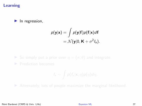
Learning
I In regression,
p(y|x) =
∫p(y|f)p(f|x)df
= N (y|0,K + σ2In).
I So simply put a prior over η = (σ, θ) and integrate.
I Prediction becomes
f? ∼∫
p(f?|x, η)p(η)dη.
I Alternately, lots of people maximize the marginal likelihood.
Remi Bardenet (CNRS & Univ. Lille) Bayesian ML 37

Learning
I In regression,
p(y|x, θ) =
∫p(y|f)p(f|x)df
= N (y|0,Kθ + σ2In).
I So simply put a prior over η = (σ, θ) and integrate.
I Prediction becomes
f? ∼∫
p(f?|x, η)p(η)dη.
I Alternately, lots of people maximize the marginal likelihood.
Remi Bardenet (CNRS & Univ. Lille) Bayesian ML 37

Beyond regression: classification8
I (Exercise) Find a simple classification model with GPs.
I Take for instance
p(y = +1|x , f ) = Bernoulli(σ(f (x))), f ∼ GP(0,K ).
I Problem: prediction is not easy anymore
p(f?|X , y, x?) =
∫p(f?|X , f, x?)p(f|X , y)df
8C. E. Rasmussen and C. K. I. Williams. Gaussian Processes for MachineLearning. MIT Press, 2006.
Remi Bardenet (CNRS & Univ. Lille) Bayesian ML 38

Beyond regression: classification8
I (Exercise) Find a simple classification model with GPs.
I Take for instance
p(y = +1|x , f ) = Bernoulli(σ(f (x))), f ∼ GP(0,K ).
I Problem: prediction is not easy anymore
p(f?|X , y, x?) =
∫p(f?|X , f, x?)p(f|X , y)df
8Rasmussen and Williams, Gaussian Processes for Machine Learning.Remi Bardenet (CNRS & Univ. Lille) Bayesian ML 38
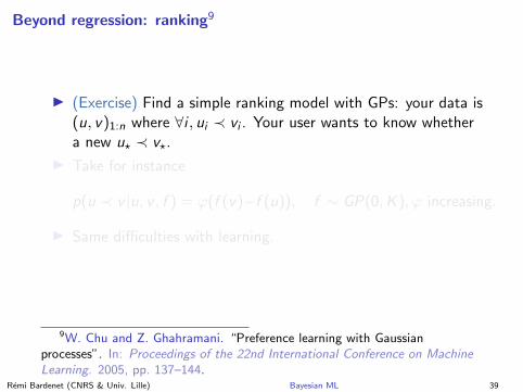
Beyond regression: ranking9
I (Exercise) Find a simple ranking model with GPs: your data is(u, v)1:n where ∀i , ui ≺ vi . Your user wants to know whethera new u? ≺ v?.
I Take for instance
p(u ≺ v |u, v , f ) = ϕ(f (v)−f (u)), f ∼ GP(0,K ), ϕ increasing.
I Same difficulties with learning.
9W. Chu and Z. Ghahramani. “Preference learning with Gaussianprocesses”. In: Proceedings of the 22nd International Conference on MachineLearning. 2005, pp. 137–144.
Remi Bardenet (CNRS & Univ. Lille) Bayesian ML 39

Beyond regression: ranking9
I (Exercise) Find a simple ranking model with GPs: your data is(u, v)1:n where ∀i , ui ≺ vi . Your user wants to know whethera new u? ≺ v?.
I Take for instance
p(u ≺ v |u, v , f ) = ϕ(f (v)−f (u)), f ∼ GP(0,K ), ϕ increasing.
I Same difficulties with learning.
9Chu and Ghahramani, “Preference learning with Gaussian processes”.Remi Bardenet (CNRS & Univ. Lille) Bayesian ML 39

Emulators of expensive models
RESEARCH ARTICLE
Bayesian Sensitivity Analysis of a Cardiac CellModel Using a Gaussian Process EmulatorEugene TY Chang1,2, Mark Strong3, Richard H Clayton1,2*
1 Insigneo Institute for in-silicoMedicine, University of Sheffield, Sheffield, United Kingdom, 2 Department ofComputer Science University of Sheffield, Sheffield, United Kingdom, 3 School of Health and RelatedResearch, University of Sheffield, Sheffield, United Kingdom
AbstractModels of electrical activity in cardiac cells have become important research tools as they
can provide a quantitative description of detailed and integrative physiology. However, car-
diac cell models have many parameters, and how uncertainties in these parameters affect
the model output is difficult to assess without undertaking large numbers of model runs. In
this study we show that a surrogate statistical model of a cardiac cell model (the Luo-Rudy
1991 model) can be built using Gaussian process (GP) emulators. Using this approach we
examined how eight outputs describing the action potential shape and action potential dura-
tion restitution depend on six inputs, which we selected to be the maximum conductances in
the Luo-Rudy 1991 model. We found that the GP emulators could be fitted to a small num-
ber of model runs, and behaved as would be expected based on the underlying physiology
that the model represents. We have shown that an emulator approach is a powerful tool for
uncertainty and sensitivity analysis in cardiac cell models.
IntroductionThe heart is an electromechanical pump.With each beat an electrical action potential originatesin the natural pacemaker, and propagates through the entire organ, acting to initiate and syn-chronise contraction. Since the publication of the first model describing the cardiac action poten-tial over 50 years ago [1], models of electrical activation and recovery in cardiac cells and tissuehave become valuable research tools. These models have explanatory power as they expressquantitatively our knowledge of the biophysical processes that generate the cardiac action poten-tial. Thus they can be used to examine the mechanisms by which gene mutations, pharmaceuti-cals and diseases act to change the properties of electrical activity in single cells and in wholetissues [2–4]. The present generation of models include detailed descriptions of the dynamics oftransmembrane current flowing through ion channels, pumps and exchangers in the cell mem-brane, coupled to detailed models of Ca2+ storage and release within the cell [4], and there hasbeen an increasing trend frommodels of animal cells towards detailed models of human atrial
PLOSONE | DOI:10.1371/journal.pone.0130252 June 26, 2015 1 / 20
a11111
OPEN ACCESS
Citation: Chang ETY, Strong M, Clayton RH (2015)Bayesian Sensitivity Analysis of a Cardiac Cell ModelUsing a Gaussian Process Emulator. PLoS ONE 10(6): e0130252. doi:10.1371/journal.pone.0130252
Academic Editor: Kevin Burrage, Oxford University,UNITED KINGDOM
Received: February 18, 2015
Accepted: May 19, 2015
Published: June 26, 2015
Copyright: © 2015 Chang et al. This is an openaccess article distributed under the terms of theCreative Commons Attribution License, which permitsunrestricted use, distribution, and reproduction in anymedium, provided the original author and source arecredited.
Data Availability Statement: All relevant data andmethods are contained within the paper and itsSupporting Information files.
Funding: This work was supported by the UKEngineering and Physical Sciences ResearchCouncil (www.epsrc.ac.uk) grant number EP/K037145/1. Mark Strong is funded by a post-doctoralfellowship grant from the National Institute for HealthResearch http://www.nihr.ac.uk (Post-DoctoralFellowship, PDF-2012-05-258). The fundingagreement ensured the authors’ independence indesigning the study, interpreting the data, writing, andpublishing the report. This report is independentresearch supported by the National Institute for
Remi Bardenet (CNRS & Univ. Lille) Bayesian ML 40

Nonparametric fits
arX
iv:1
204.
2272
v2 [
astr
o-ph
.CO
] 1
0 Ju
l 201
2
Gaussian Process Cosmography
Arman Shafieloo1, Alex G. Kim2, Eric V. Linder1,2,31 Institute for the Early Universe WCU, Ewha Womans University, Seoul, Korea
2 Lawrence Berkeley National Laboratory, Berkeley, CA 94720, USA and3 University of California, Berkeley, CA 94720, USA
(Dated: July 11, 2012)
Gaussian processes provide a method for extracting cosmological information from observationswithout assuming a cosmological model. We carry out cosmography – mapping the time evolutionof the cosmic expansion – in a model-independent manner using kinematic variables and a geometricprobe of cosmology. Using the state of the art supernova distance data from the Union2.1 compila-tion, we constrain, without any assumptions about dark energy parametrization or matter density,the Hubble parameter and deceleration parameter as a function of redshift. Extraction of theserelations is tested successfully against models with features on various coherence scales, subject tocertain statistical cautions.
I. INTRODUCTION
Cosmic acceleration is a fundamental mystery of greatinterest and importance to understanding cosmology,gravitation, and high energy physics. The cosmic ex-pansion rate is slowed down by gravitationally attractivematter and sped up by some other, unknown contribu-tion to the dynamical equations. While great effort isbeing put into identifying the source of this extra darkenergy contribution, the overall expansion behavior alsoholds important clues to origin, evolution, and presentstate of our universe.Indeed, by studying the expansion as a whole one
sidesteps the issue of exactly how to divide the gravi-tationally attractive (e.g. the imperfectly known matterdensity) and the accelerating contributions, and whetherthey are independent or have some interaction (see, e.g.,[1–3]). By concentrating on the kinematic variables – theexpansion properties as a function of redshift z or scalefactor a = 1/(1 + z) – one does not need to know the in-ternal structure of the field equations, i.e. the dynamics.The clarity and focus on kinematics trades off against theloss of information on the specific dynamics.Another gain comes from using geometric measure-
ments – cosmic-distance variables that do not depend onthe particular forces and mass densities. The sensitiv-ity of Type Ia supernova measurements of the distance-redshift relation to the deceleration parameter was usedto discover the accelerated expansion [4, 5]. Other probessuch as gravitational lensing, galaxy-clustering statis-tics, cluster-mass abundances, etc. provide valuable in-formation, but are dependent on non-kinematic variables.Some techniques, such as distances from baryon acousticoscillations and Sunyaev-Zel’dovich effects in clusters, areon the fence, nominally geometric but having implicit de-pendence on the gravitational interaction of matter andso the force law dynamics.Given distance and redshift measurements, the cosmic
expansion rate is related by a derivative of the data, andthe deceleration parameter by a further derivative. Thisis problematic for data with real world noise, as the dif-ferentiation further amplifies the noise. Various smooth-
ing procedures have been suggested, e.g. [6], but tend toinduce bias in the function reconstruction due to para-metric restriction of the behavior or to have poor errorcontrol. Using a general orthonormal basis or principalcomponent analysis is another approach, to describe thedistance-redshift relation (e.g. [7]) or the deceleration pa-rameter [8], or using a correlated prior for smoothness onthe dark energy equation of state [9], but in practice afinite (and small) number of modes is significant beyondthe prior, essentially reducing to a parametric approach.Gaussian processes [10] offer an interesting possibility forimproving this situation.
Gaussian processes (GP) have been used recently [11–13] in a dynamical reconstruction, going from a set ofrealizations of the equation of state parameter w(z) ofthe dark energy component forward to comparison of thederived distance-relation to the distance data. The com-parison was carried out through a Markov Chain MonteCarlo (MCMC) assessment of likelihoods. Note that theGP interpolation does not occur between data points butrather on an arbitrary grid of some possibly unmeasuredquantity. This approach is intriguing, but relies on sep-aration of the matter density from the dark energy be-havior, i.e. it works within a dynamical framework.
The approach in this paper takes a fundamentally dif-ferent path. We begin with the observations of supernovadistances and here consider only kinematic quantities.Modeling the cosmic distance relation as a smooth kine-matic function drawn from a GP, the value of the functionat any redshift is then predicted directly through testingthe GP model against the data. The cosmic expansioncan then be extracted from the means and covariance ma-trices of the Gaussian process realizations (weighted bya posterior) directly for quantities related linearly to theoriginal GP, even through derivatives. This allows us toprobe the rate and acceleration of the cosmic expansionin a highly model-independent manner (at the price offocusing on only this type of information). One can viewthis as a top-down approach, complementary with thebottom-up approach of starting with theoretical quanti-ties and working toward the data, and then applying alikelihood comparison.
Remi Bardenet (CNRS & Univ. Lille) Bayesian ML 41
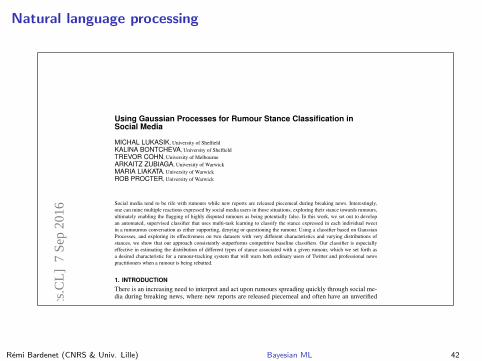
Natural language processing
Using Gaussian Processes for Rumour Stance Classification inSocial Media
MICHAL LUKASIK, University of SheffieldKALINA BONTCHEVA, University of SheffieldTREVOR COHN, University of MelbourneARKAITZ ZUBIAGA, University of WarwickMARIA LIAKATA, University of WarwickROB PROCTER, University of Warwick
Social media tend to be rife with rumours while new reports are released piecemeal during breaking news. Interestingly,one can mine multiple reactions expressed by social media users in those situations, exploring their stance towards rumours,ultimately enabling the flagging of highly disputed rumours as being potentially false. In this work, we set out to developan automated, supervised classifier that uses multi-task learning to classify the stance expressed in each individual tweetin a rumourous conversation as either supporting, denying or questioning the rumour. Using a classifier based on GaussianProcesses, and exploring its effectiveness on two datasets with very different characteristics and varying distributions ofstances, we show that our approach consistently outperforms competitive baseline classifiers. Our classifier is especiallyeffective in estimating the distribution of different types of stance associated with a given rumour, which we set forth asa desired characteristic for a rumour-tracking system that will warn both ordinary users of Twitter and professional newspractitioners when a rumour is being rebutted.
1. INTRODUCTIONThere is an increasing need to interpret and act upon rumours spreading quickly through social me-dia during breaking news, where new reports are released piecemeal and often have an unverifiedstatus at the time of posting. Previous research has posited the damage that the diffusion of falserumours can cause in society, and that corrections issued by news organisations or state agenciessuch as the police may not necessarily achieve the desired effect sufficiently quickly [Lewandowskyet al. 2012; Procter et al. 2013a]. Being able to determine the accuracy of reports is therefore crucialin these scenarios. However, the veracity of rumours in circulation is usually hard to establish [All-port and Postman 1947], since as many views and testimonies as possible need to be assembled andexamined in order to reach a final judgement. Examples of rumours that were later disproven, afterbeing widely circulated, include a 2010 earthquake in Chile, where rumours of a volcano eruptionand a tsunami warning in Valparaiso spawned on Twitter [Mendoza et al. 2010]. Another exampleis the England riots in 2011, where false rumours claimed that rioters were going to attack Birming-ham’s Children’s Hospital and that animals had escaped from London Zoo [Procter et al. 2013b].
Previous work by ourselves and others has argued that looking at how users in social mediaorient to rumours is a crucial first step towards making an informed judgement on the veracity of arumourous report [Zubiaga et al. 2016; Tolmie et al. 2015; Mendoza et al. 2010]. For example, in thecase of the riots in England in August 2011, Procter et al. manually analysed the stance expressed byusers in social media towards rumours [Procter et al. 2013b]. Each tweet discussing a rumour wasmanually categorised as supporting, denying or questioning it. It is obvious that manual methodshave their disadvantages in that they do not scale well; the ability to perform stance categorisationof tweets in an automated way would be of great use in tracking rumours, flagging those that arelargely denied or questioned as being more likely to be false.
Determining the stance of social media posts automatically has been attracting increasing interestin the scientific community in recent years, as this is a useful first step towards more in-depth rumouranalysis:
— It can help detect rumours and flag them as such more quickly [Zhao et al. 2015].— It is useful for tracking public opinion about rumours and hence for monitoring their wider effect
on society.
arX
iv:1
609.
0196
2v1
[cs
.CL
] 7
Sep
201
6
Remi Bardenet (CNRS & Univ. Lille) Bayesian ML 42

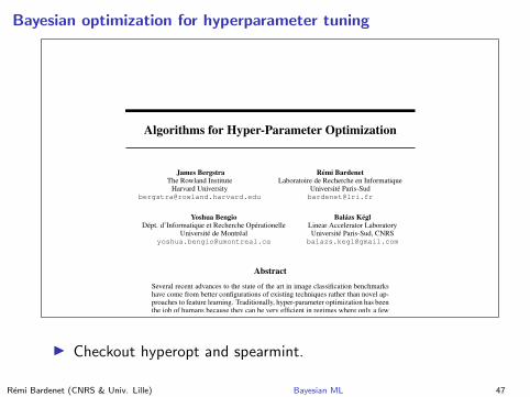
Bayesian optimization for hyperparameter tuning
Algorithms for Hyper-Parameter Optimization
James BergstraThe Rowland Institute
Harvard [email protected]
Remi BardenetLaboratoire de Recherche en Informatique
Universite [email protected]
Yoshua BengioDept. d’Informatique et Recherche Operationelle
Universite de [email protected]
Balazs KeglLinear Accelerator LaboratoryUniversite Paris-Sud, CNRS
Abstract
Several recent advances to the state of the art in image classification benchmarkshave come from better configurations of existing techniques rather than novel ap-proaches to feature learning. Traditionally, hyper-parameter optimization has beenthe job of humans because they can be very efficient in regimes where only a fewtrials are possible. Presently, computer clusters and GPU processors make it pos-sible to run more trials and we show that algorithmic approaches can find betterresults. We present hyper-parameter optimization results on tasks of training neu-ral networks and deep belief networks (DBNs). We optimize hyper-parametersusing random search and two new greedy sequential methods based on the ex-pected improvement criterion. Random search has been shown to be sufficientlyefficient for learning neural networks for several datasets, but we show it is unreli-able for training DBNs. The sequential algorithms are applied to the most difficultDBN learning problems from [1] and find significantly better results than the bestpreviously reported. This work contributes novel techniques for making responsesurface models P (y|x) in which many elements of hyper-parameter assignment(x) are known to be irrelevant given particular values of other elements.
1 Introduction
Models such as Deep Belief Networks (DBNs) [2], stacked denoising autoencoders [3], convo-lutional networks [4], as well as classifiers based on sophisticated feature extraction techniqueshave from ten to perhaps fifty hyper-parameters, depending on how the experimenter chooses toparametrize the model, and how many hyper-parameters the experimenter chooses to fix at a rea-sonable default. The difficulty of tuning these models makes published results difficult to reproduceand extend, and makes even the original investigation of such methods more of an art than a science.
Recent results such as [5], [6], and [7] demonstrate that the challenge of hyper-parameter opti-mization in large and multilayer models is a direct impediment to scientific progress. These workshave advanced state of the art performance on image classification problems by more concertedhyper-parameter optimization in simple algorithms, rather than by innovative modeling or machinelearning strategies. It would be wrong to conclude from a result such as [5] that feature learningis useless. Instead, hyper-parameter optimization should be regarded as a formal outer loop in thelearning process. A learning algorithm, as a functional from data to classifier (taking classificationproblems as an example), includes a budgeting choice of how many CPU cycles are to be spenton hyper-parameter exploration, and how many CPU cycles are to be spent evaluating each hyper-parameter choice (i.e. by tuning the regular parameters). The results of [5] and [7] suggest thatwith current generation hardware such as large computer clusters and GPUs, the optimal alloca-
1
Remi Bardenet (CNRS & Univ. Lille) Bayesian ML 43

Bayesian optimization
I Goal is to minimize a noisy f with N iterations, N small.
I Key application: find the hyperparameters of your MLalgorithm that minimize the validation error.
I Idea is to sequentiallyI update your model on f ,I optimize an aquisition criterion.
I Check out notebook 03 onhttps://github.com/rbardenet/bnp-course.
Remi Bardenet (CNRS & Univ. Lille) Bayesian ML 44

An example in 1D
0 2 4 6 8 10
5
0
5
10
targ
et
0 2 4 6 8 100.00
0.02
0.04
0.06
0.08
0.10
0.12
0.14
0.16
EI
Remi Bardenet (CNRS & Univ. Lille) Bayesian ML 45

An example in 1D
0 2 4 6 8 10
5
0
5
10
targ
et
0 2 4 6 8 100.00
0.02
0.04
0.06
0.08
0.10
0.12
EI
Remi Bardenet (CNRS & Univ. Lille) Bayesian ML 45

An example in 1D
0 2 4 6 8 10
5
0
5
10
targ
et
0 2 4 6 8 100.00
0.01
0.02
0.03
0.04
0.05
0.06
0.07
0.08
0.09
EI
Remi Bardenet (CNRS & Univ. Lille) Bayesian ML 45

An example in 1D
0 2 4 6 8 10
5
0
5
10
targ
et
0 2 4 6 8 100.00
0.01
0.02
0.03
0.04
0.05
0.06
0.07
0.08
0.09
EI
Remi Bardenet (CNRS & Univ. Lille) Bayesian ML 45

An example in 1D
0 2 4 6 8 10
5
0
5
10
targ
et
0 2 4 6 8 100.00
0.01
0.02
0.03
0.04
0.05
0.06
0.07
EI
Remi Bardenet (CNRS & Univ. Lille) Bayesian ML 45

An example in 1D
0 2 4 6 8 10
5
0
5
10
targ
et
0 2 4 6 8 100.000
0.005
0.010
0.015
0.020
0.025
0.030
0.035
0.040
EI
Remi Bardenet (CNRS & Univ. Lille) Bayesian ML 45

An example in 1D
0 2 4 6 8 10
5
0
5
10
targ
et
0 2 4 6 8 100.000
0.005
0.010
0.015
0.020
0.025
0.030
EI
Remi Bardenet (CNRS & Univ. Lille) Bayesian ML 45

An example in 1D
0 2 4 6 8 10
5
0
5
10
targ
et
0 2 4 6 8 100.002
0.000
0.002
0.004
0.006
0.008
0.010
0.012
0.014
0.016
EI
Remi Bardenet (CNRS & Univ. Lille) Bayesian ML 45

An example in 1D
0 2 4 6 8 10
5
0
5
10
targ
et
0 2 4 6 8 100.000
0.002
0.004
0.006
0.008
0.010
EI
Remi Bardenet (CNRS & Univ. Lille) Bayesian ML 45

An example in 1D
0 2 4 6 8 10
5
0
5
10
targ
et
0 2 4 6 8 100.000
0.001
0.002
0.003
0.004
0.005
0.006
EI
Remi Bardenet (CNRS & Univ. Lille) Bayesian ML 45

Popular aquisition criteria
Expected improvement10
EI(z) = E(
max(mN − f (z), 0)|(x , y)1:n
),
where mN = min16i6N f (xi ).
An easy computation yields
EI(x) = σ(x)(uΦ(u) + ϕ(u)
), (3)
whereu = (mn − m(x))/σ(x),
and Φ and ϕ denote the cdf and pdf of the N (0, 1) distribution.
10D. R. Jones. “A Taxonomy of Global Optimization Methods Based onResponse Surfaces”. In: Journal of Global Optimization 21 (2001),pp. 345–383.
Remi Bardenet (CNRS & Univ. Lille) Bayesian ML 46

GP-UCB (Srinivas et al., 2010)
GP-UCB
GP-UCB(z) = m(z) + βσ(z).
I If β properly tuned, can use bandit results.
I First criterion to give application theoretical results.
Remi Bardenet (CNRS & Univ. Lille) Bayesian ML 46
Bayesian optimization for hyperparameter tuning
Algorithms for Hyper-Parameter Optimization
James BergstraThe Rowland Institute
Harvard [email protected]
Remi BardenetLaboratoire de Recherche en Informatique
Universite [email protected]
Yoshua BengioDept. d’Informatique et Recherche Operationelle
Universite de [email protected]
Balazs KeglLinear Accelerator LaboratoryUniversite Paris-Sud, CNRS
Abstract
Several recent advances to the state of the art in image classification benchmarkshave come from better configurations of existing techniques rather than novel ap-proaches to feature learning. Traditionally, hyper-parameter optimization has beenthe job of humans because they can be very efficient in regimes where only a fewtrials are possible. Presently, computer clusters and GPU processors make it pos-sible to run more trials and we show that algorithmic approaches can find betterresults. We present hyper-parameter optimization results on tasks of training neu-ral networks and deep belief networks (DBNs). We optimize hyper-parametersusing random search and two new greedy sequential methods based on the ex-pected improvement criterion. Random search has been shown to be sufficientlyefficient for learning neural networks for several datasets, but we show it is unreli-able for training DBNs. The sequential algorithms are applied to the most difficultDBN learning problems from [1] and find significantly better results than the bestpreviously reported. This work contributes novel techniques for making responsesurface models P (y|x) in which many elements of hyper-parameter assignment(x) are known to be irrelevant given particular values of other elements.
1 Introduction
Models such as Deep Belief Networks (DBNs) [2], stacked denoising autoencoders [3], convo-lutional networks [4], as well as classifiers based on sophisticated feature extraction techniqueshave from ten to perhaps fifty hyper-parameters, depending on how the experimenter chooses toparametrize the model, and how many hyper-parameters the experimenter chooses to fix at a rea-sonable default. The difficulty of tuning these models makes published results difficult to reproduceand extend, and makes even the original investigation of such methods more of an art than a science.
Recent results such as [5], [6], and [7] demonstrate that the challenge of hyper-parameter opti-mization in large and multilayer models is a direct impediment to scientific progress. These workshave advanced state of the art performance on image classification problems by more concertedhyper-parameter optimization in simple algorithms, rather than by innovative modeling or machinelearning strategies. It would be wrong to conclude from a result such as [5] that feature learningis useless. Instead, hyper-parameter optimization should be regarded as a formal outer loop in thelearning process. A learning algorithm, as a functional from data to classifier (taking classificationproblems as an example), includes a budgeting choice of how many CPU cycles are to be spenton hyper-parameter exploration, and how many CPU cycles are to be spent evaluating each hyper-parameter choice (i.e. by tuning the regular parameters). The results of [5] and [7] suggest thatwith current generation hardware such as large computer clusters and GPUs, the optimal alloca-
1
I Checkout hyperopt and spearmint.
Remi Bardenet (CNRS & Univ. Lille) Bayesian ML 47

Going further: Hyperopt across datasets10
10R. Bardenet et al. “Collaborative hyperparameter tuning”. In:International Conference on Machine Learning (ICML). Atlanta, Georgia, 2013.
Remi Bardenet (CNRS & Univ. Lille) Bayesian ML 48

Some useful hyperlinks
I Textbook by C. E. Rasmussen and C. K. I. Williams.Gaussian Processes for Machine Learning. MIT Press, 2006,I great for understanding, methods, pointers to ML and stats.
I Videolecture by C. Rasmussen.I lecture notes by P. Orbanz. Lecture notes on Bayesian
nonparametrics. 2014.I mathematically clean, without losing the focus on ML.
Remi Bardenet (CNRS & Univ. Lille) Bayesian ML 49

Some open issues
I Fully Bayesian scalable approaches!
I Natural approaches to constrained GPs.
I Links with other models based on Gaussians and geometry.
Back to the roots
I Formulate HT across datasets and algorithms as a posteriorexpected loss problem, including computational constraints.
I Solve resulting dynamic programming problem.
Remi Bardenet (CNRS & Univ. Lille) Bayesian ML 50

References I
Bardenet, R. et al. “Collaborative hyperparameter tuning”. In:International Conference on Machine Learning (ICML). Atlanta,Georgia, 2013.
Blei, D. M., A. Kucukelbir, and J. D. McAuliffe. “Variationalinference: A review for statisticians”. In: Journal of the AmericanStatistical Association 112.518 (2017), pp. 859–877.
Chu, W. and Z. Ghahramani. “Preference learning with Gaussianprocesses”. In: Proceedings of the 22nd International Conferenceon Machine Learning. 2005, pp. 137–144.
Douc, R., E. Moulines, and D. Stoffer. Nonlinear time series.Chapman-Hall, 2014.
Jones, D. R. “A Taxonomy of Global Optimization Methods Basedon Response Surfaces”. In: Journal of Global Optimization 21(2001), pp. 345–383.
Orbanz, P. Lecture notes on Bayesian nonparametrics. 2014.
Remi Bardenet (CNRS & Univ. Lille) Bayesian ML 51

References II
Parmigiani, G. and L. Inoue. Decision theory: principles andapproaches. Vol. 812. John Wiley & Sons, 2009.
Rasmussen, C. E. and C. K. I. Williams. Gaussian Processes forMachine Learning. MIT Press, 2006.
Robert, C. P. The Bayesian choice: from decision-theoreticfoundations to computational implementation. Springer Science& Business Media, 2007.
Robert, C. P. and G. Casella. Monte Carlo Statistical Methods.New York: Springer-Verlag, 2004.
Stigler, S. M. “The epic story of maximum likelihood”. In:Statistical Science (2007), pp. 598–620.
Wald, A. Statistical decision functions. Wiley, 1950.
Remi Bardenet (CNRS & Univ. Lille) Bayesian ML 52
Recommended


![arXiv:1905.09967v1 [physics.app-ph] 23 May 2019 · 1Thales Research and Technology, 1, Avenue Augustin Fresnel, 91767 Palaiseau, France 2IEMN, University of Lille, CNRS UMR8520, Avenue](https://img.dokumen.tips/doc/110x75/5fd50db1317c52792d6c01ca/arxiv190509967v1-23-may-2019-1thales-research-and-technology-1-avenue-augustin.jpg)