Bayesian Inference of Weibull
Distribution Based on Left Truncated and
Right Censored Data
Debasis Kundu1 & Debanjan Mitra2
Abstract
This article deals with the Bayesian inference of the unknown parameters of the
Weibull distribution based on the left truncated and right censored data. It is assumed
that the scale parameter of the Weibull distribution has a gamma prior. The shape pa-
rameter may be known or unknown. If the shape parameter is unknown, it is assumed
that it has a very general log-concave prior distribution. When the shape parameter
is unknown, the closed form expression of the Bayes estimates cannot be obtained.
We propose to use Gibbs sampling procedure to compute the Bayes estimates and the
associated highest posterior density credible intervals. Two data sets, one simulated
and one real life, have been analyzed to show the effectiveness of the proposed method,
and the performances are quite satisfactory. We further develop posterior predictive
density of an item still in use. Based on the predictive density we provide predic-
tive survival probability at a certain point along with the associated highest posterior
density credible interval and also the expected number of failures in a given interval.
Key Words and Phrases: Fisher information matrix; maximum likelihood estimators;
Gibbs sampling; Prior distribution; Posterior analysis; Credible intervals.
AMS 2000 Subject Classification: Primary 62F10; Secondary: 62H10
1Department of Mathematics and Statistics, Indian Institute of Technology Kanpur, Kanpur,
Pin 208016, India. e-mail: [email protected].
2Operations Management, Quantitative Methods and Information Systems, Indian Institute
of Management Udaipur, India.
1

1 Introduction
The problem was mainly motivated from an example provided in Hong et al. (2009). The
problem has been stated as follows. There are approximately 150,000 high-voltage power
transformers in service in different parts of U.S. These transformers have been installed
at different times in the past, and the failure times of the these transformers are random
in nature. Naturally for the transformers which are still in service, the prediction of the
remaining life of any transformer and also the expected number of failures within a given
interval are two important issues.
The energy company started careful record keeping in 1980. The complete information
of the lifetime of the transformers installed after 1980 are available. The information on
transformers installed before 1980 and failed after 1980 are also available. Although, no
information on units which were installed before 1980 and also failed before 1980, is available.
The authors analyzed the data based on the assumption that the lifetime distribution of the
transformers follow a two-parameter Weibull distribution. They obtained the maximum
likelihood estimators (MLEs) of the unknown parameters, and mentioned that the two-
parameter Weibull distribution provided an excellent fit to the data set.
Recently Balakrishnan and Mitra (2012) considered the same problem and provided a
detailed analysis of the model. In this connection, see also Balakrishnan and Mitra (2011,
2013, 2014). They proposed to use the expectation maximization (EM) algorithm to com-
pute the MLEs of the unknown parameters and also provided the confidence intervals of
the unknown parameters based on the missing information principle. They had performed
extensive simulations experiments to observe the behavior of the proposed EM algorithm.
It is observed that if the truncation proportion is high, and the sample size is not very large
then the EM algorithm may not converge. Moreover, in some instances, the EM algorithm
2

provides highly biased estimates, and based on the biased estimates, the observed Fisher
information matrix may produce negative variances of the MLEs. Hence, the MLEs can be
misleading sometime.
Due to these reasons, it seems Bayesian inference is a reasonable alternative. Here, the
data obtained are left truncated and right censored. We consider the Bayesian inference of
the above mentioned problem. It is assumed that the lifetime of the units have a Weibull
distribution with probability density function (PDF)
f(t;α, λ) ={αλtα−1e−λtα if t > 0
0 if t ≤ 0.(1)
Here α > 0 and λ > 0 are the shape and scale parameters, respectively. From now on the
Weibull distribution with the PDF (1) will be denoted by WE(α, λ)
For developing the Bayesian inference on the parameters of the lifetime distribution, we
need to make some assumptions on the prior distribution. If the shape parameter α is known,
the natural choice on the scale parameter λ is the conjugate prior. In this case the Bayes
estimate of the scale parameter can be obtained in explicit form. If the shape parameter is
not known, the continuous conjugate prior on α does not exist, see for example Kaminskiy
and Krivtson (2005). In this case we use the same conjugate prior on λ, even when α
was unknown. No specific prior on α is assumed. It is assumed that the prior on α has a
support on (0,∞) and it has a log-concave PDF. It may be mentioned that many well-known
distributions, like normal, gamma, Weibull, log-normal may have log-concave PDFs. The
Weibull distribution is one of the most commonly used distribution in reliability of lifetime
analysis. It thus have been widely studied even in the Bayesian framework. Interested
readers are referred to Erto (1980), Berger and Sun (1993), Hamada et al. (2008), Kundu
(2008), Pradhan and Kundu (2014), and the references cited therein.
It is observed that when the shape parameter is known, the Bayes estimate of the scale
3

parameter and the associated credible interval can be obtained in explicit form. If the
shape parameter is unknown, the Bayes estimates of the unknown parameters cannot be
obtained in closed form. We propose to use Gibbs sampling technique to compute the
Bayes estimates and the associated highest posterior density (HPD) credible intervals of the
unknown parameters. We also consider the prediction distribution of the remaining lifetime
of an item, which has not yet failed. Based on the predictive distribution, we obtain the
predictive survival probability at a future time point of an unit which has not yet failed,
and also compute the associated HPD credible interval based on Gibbs sampling technique.
We further compute the expected number of units failing in each future interval of time.
The analysis of two data sets, one simulated and one real life, are performed to observe
the behavior and the effectiveness of the proposed method. The performances are quite
satisfactory.
Rest of the paper is organized as follows. In Section 2, we provide the problem for-
mulation and necessary assumptions. Bayes estimates and the associated credible intervals
are provided in Section 3. In Section 4, the analysis of two data sets have been presented.
Prediction issues are discussed in Section 5. Finally, we conclude the paper in Section 6.
2 Problem Formulation and Assumptions
Items are put on a test at different time points. Let the effective lifetime of an item be
denoted by a random variable T . For each item there is one pre fixed time point τL, and
the failure time of an item is observable only if T > τL. Note that τL may depend on the
item, and an item may be put on test after τL. If an item has been put on a test before
τL and it has not failed till τL, or if it has been put on a test after τL, it may be censored
at τR > τL. The information regarding an item is available only if it fails after τL, or it is
being censored after τL. Therefore, the information regarding the number of failures before
4

the left truncation point is not available.
We use the following notations in this paper. Let Ti denote the lifetime random variable
of the i-th item, and ti denote the corresponding observed value. Let δi denote the censoring
indicator, i.e. δi is 0 if the i-th observation is censored, and 1, if the i-th item is not censored,
and τiL denote the left truncation time. Moreover, let νi denote the truncation indicator of
the i-th item, i.e. νi is 0, if an observation is truncated, and 1, if it is not truncated. Let S1
and S2 be two index sets. If i ∈ S1, it implies that the i-th unit has been put into test after
τiL, and if i ∈ S2, it means i-th unit has been put into test before τiL, but it has survived
till τiL. We further denote S = S1 ∪ S2, i.e. the set of items about which information is
available.
If f(t;θ) and F (t;θ) denote the probability density function (PDF) and cumulative
distribution function (CDF) of T , respectively, then based on the observations {(ti, δi); i ∈
S}, the likelihood function becomes
L(θ) =∏
i∈S
{f(ti;θ)}δiνi {1− F (ti;θ)}
(1−δi)νi
{f(ti;θ)
1− F (τiL;θ)
}δi(1−νi) { 1− F (ti;θ)
1− F (τiL;θ)
}(1−δi)(1−νi)
=∏
i∈S1
{f(ti;θ)}δi {1− F (ti;θ)}
1−δi ×∏
i∈S2
{f(ti;θ)
1− F (τiL;θ)
}δi { 1− F (ti;θ)
1− F (τiL;θ)
}1−δi
(2)
In this paper it is assumed that T follows (∼) WE(α, λ), therefore, based on the observations
{(ti, δi, νi); i = 1, . . . , n}, and with the associated τiL, the log-likelihood function becomes
L(α, λ|Data) =∏
i∈S11
αλtα−1i e−λtαi ×
∏
i∈S10
e−λtαi ×∏
i∈S21
αλtα−1i e−λ(tαi −τα
iL)×
∏
i∈S20
e−λ(tαi −ταiL
). (3)
Here S11 = {i; i ∈ S1, δi = 1}, S10 = {i; i ∈ S1, δi = 0}, S21 = {i; i ∈ S2, δi = 1},
S20 = {i; i ∈ S2, δi = 0}. We denote the number of elements in S11, S10, S21 and S20 as n11,
n10, n21, n20, respectively and n = n11 + n10 + n21 + n20, m = n11 + n21. Further we denote
Sc = S11 ∪ S21 and note that S2 = S21 ∪ S20. With these notations, (3) becomes
L(α, λ|Data) = αmλm ×∏
i∈Sc
tα−1i × e
−λ(∑
i∈Stαi −∑
i∈S2ταiL
). (4)
5
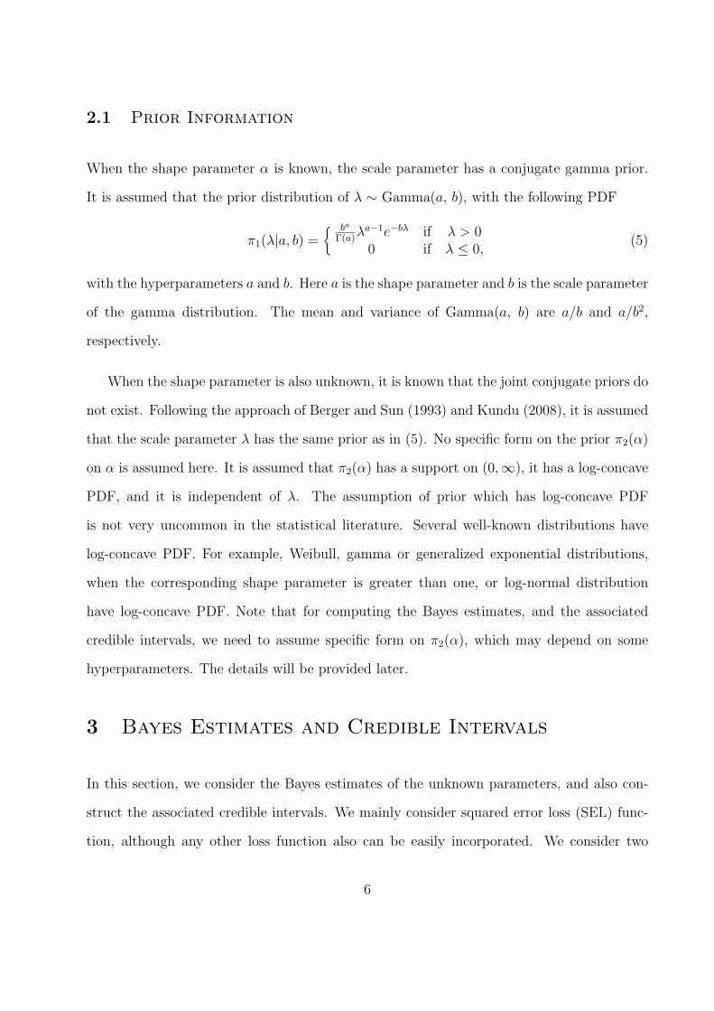
2.1 Prior Information
When the shape parameter α is known, the scale parameter has a conjugate gamma prior.
It is assumed that the prior distribution of λ ∼ Gamma(a, b), with the following PDF
π1(λ|a, b) ={ ba
Γ(a)λa−1e−bλ if λ > 00 if λ ≤ 0,
(5)
with the hyperparameters a and b. Here a is the shape parameter and b is the scale parameter
of the gamma distribution. The mean and variance of Gamma(a, b) are a/b and a/b2,
respectively.
When the shape parameter is also unknown, it is known that the joint conjugate priors do
not exist. Following the approach of Berger and Sun (1993) and Kundu (2008), it is assumed
that the scale parameter λ has the same prior as in (5). No specific form on the prior π2(α)
on α is assumed here. It is assumed that π2(α) has a support on (0,∞), it has a log-concave
PDF, and it is independent of λ. The assumption of prior which has log-concave PDF
is not very uncommon in the statistical literature. Several well-known distributions have
log-concave PDF. For example, Weibull, gamma or generalized exponential distributions,
when the corresponding shape parameter is greater than one, or log-normal distribution
have log-concave PDF. Note that for computing the Bayes estimates, and the associated
credible intervals, we need to assume specific form on π2(α), which may depend on some
hyperparameters. The details will be provided later.
3 Bayes Estimates and Credible Intervals
In this section, we consider the Bayes estimates of the unknown parameters, and also con-
struct the associated credible intervals. We mainly consider squared error loss (SEL) func-
tion, although any other loss function also can be easily incorporated. We consider two
6

cases separately, namely when the (a) shape parameter is known and (b) shape parameter
is unknown.
3.1 Shape Parameter Known
In this case based on the prior distribution on λ as in (5), and from the likelihood function
(3), the posterior distribution of λ can be written as
π(λ|α, data) ∝ λa+m−1e−λ(b+
∑i∈S
tαi −∑
i∈S2ταiL
). (6)
Therefore, the Bayes estimate of λ under the SEL function becomes
λ =a+m
b+∑
i∈S tαi −
∑i∈S2
ταiL. (7)
Since λ follows a posteriori gamma distribution, symmetric credible interval can be obtained
in terms of incomplete gamma function. If a is an integer, then chi-squared table can be
used to construct symmetric credible interval of λ. In general Gibbs sampling technique also
can be used to construct HPD credible interval of λ, details will be provided in the next
section.
3.2 Shape Parameter Unknown
In this case we consider the case when both the parameters are unknown. In this case based
on the independent priors π1(λ|a, b) and π2(α), the posterior distribution of α and λ given
the data can be written as
π(α, λ|data) =L(α, λ|data)π1(λ)π2(α)∫
∞
0
∫∞
0 L(α, λ|data)π1(λ)π2(α)dαdλ. (8)
Therefore, the Bayes estimate of any function of α and λ, say g(α, λ), under SEL function,
can be obtained as
gB(α, λ) =
∫∞
0
∫∞
0 g(α, λ)L(α, λ|data)π1(λ)π2(α)dαdλ∫∞
0
∫∞
0 L(α, λ|data)π1(λ)π2(α)dαdλ. (9)
7

It is immediate that except for trivial cases, even if π2(α) is completely known gB(α, λ)
cannot be obtained analytically. We propose to use the following two approximation to
compute the Bayes estimate and the associated credible interval.
3.2.1 Gibbs Sampling Procedure
In this section we propose to use Gibbs sampling procedure under certain restrictions on
the data sequence, to compute the Bayes estimates of the unknown parameters, and also
to compute the associated credible intervals. A posteriori, the conditional distribution of
λ given α and data has already been obtained as Gamma(a + m, b +∑
i∈S tαi −
∑i∈S2
ταiL).
Therefore, the posterior density function of α given the data can be written as
π(α|data) ∝ π2(α)αm∏
i∈Sc
tα−1i ×
1
(b+∑
i∈S tαi −
∑i∈S2
ταiL)a+m
. (10)
The following result will be useful for further development
Theorem 1: If
u(α) =
∑
i∈S
tαi (ln ti)2 −
∑
i∈S2
ταiL(ln τiL)2
×
b+
∑
i∈S
tαi −∑
i∈S2
ταiL
−
∑
i∈S
tαi ln ti −∑
i∈S2
ταiL ln τiL
2
,
(11)
and for all α > 0, u(α) ≥ 0, then π(α|data) is log-concave.
Proof: See in the Appendix.
Therefore, if the data sequence satisfies the condition (11), then using the idea of Geman
and Geman (1984), we can use the following procedure to compute the Bayes estimates and
also compute the associated credible intervals.
Algorithm 1:
Step 1: Generate α1 from the log-concave PDF (10) using the method proposed by Devroye
(1984). Alternatively, the approximation proposed by Kundu (2008) also can be used to
8

generate α1.
Step 2: Generate λ1 ∼ Gamma((a+m, b+∑
i∈S tαi −
∑i∈S2
ταiL)
Step 3: Repeat Step 1 and Step 2, M times, and generate (α1, λ1), . . . , (αM , λM).
Step 4: Obtain the Bayes estimates of α and λ with respect to SEL function as
αBG =1
M
M∑
k=1
αk and λBG =1
M
M∑
k=1
λk,
respectively.
Step 5: To compute 100(1− 2β)% highest posterior density (HPD) credible intervals of α
and λ, order α1, . . . , αM and λ1, . . . , λM , as follows: α1 < . . . < αM and β1 < . . . < βM .
Then construct 100(1− 2β)% credible intervals of α and λ for j = 1, . . . ,M , as
(α[jβ], α[j(1−β)]) and (λ[jβ], λ[j(1−β)]),
respectively. Where [x] denotes the maximum integer less than or equal to x. Hence the HPD
credible interval can be obtained by choosing that interval which has the shortest length.
3.2.2 Importance Sampling
In this section we propose to use importance sampling technique to compute the Bayes
estimate and the associated credible interval of g(α, λ) a function of the unknown parameters,
when the data sequence does not satisfy the condition (11). We rewrite the posterior density
function of α, (10), as follows:
π(α|data) = kπ2(α)αm∏
i∈Sc
tα−1i ×
1
(b+∑
i∈S tαi )
a+m× h(α), (12)
where
h(α) =
(b+
∑i∈S t
αi
b+∑
i∈S tαi −
∑i∈S2
ταiL
)a+m
9

and k is the normalizing constant.
The following result will be useful for further development.
Theorem 2: If we define,
π1(α|data) ∝ π2(α)αm∏
i∈Sc
tα−1i ×
1
(b+∑
i∈S tαi )
a+m, (13)
then π1(α|data) is log-concave.
Proof: The proof can be obtained along the same line as the proof of Theorem 1, hence it
is omitted..
The following algorithm can be used to compute Bayes estimate and also to construct
the associated credible interval of g(α, λ).
Algorithm 2:
Step 1: Generate α1 ∼ π1(α|data) using the method proposed by Devroye (1984). Alterna-
tively, the approximation proposed by Kundu (2008) also can be used to generate α1.
Step 2: Generate λ1 ∼ Gamma(a+m, b+∑
i∈S tαi −
∑i∈S2
ταiL).
Step 3: Repeat Step 1 and Step 2, M times, and generate (α1, λ1), . . . , (αM , λM).
Step 4: A simulation-consistent estimator Bayes estimator of g(α, λ) can be obtained as
gBI =
∑Mi=1 g(αi, λi)h(αi)∑M
j=1 h(αj).
Step 5: Now to construct a 100(1−γ)% HPD credible interval of g(α, λ), first let us denote
gi = g(αi, λi) and wi =h(αi)∑Mj=1 h(αi)
; for i = 1, . . . ,M.
Rearrange {(g1, w1), . . . , (gM , wM)} as {(g(1), w[1]), . . . , (g(M), w[M ])}, where g(1) < . . . , g(M).
In this case, w[i]’s are not ordered, they are just associated with g(i). Let Mp be the integer
10

satisfyingMp∑
i=1
w[i] ≤ p <Mp+1∑
i=1
w[i]
for 0 < p < 1. A 100(1 − γ)% HPD credible interval of g(α, λ) can be obtained as
(g(Mb), g(Mb+1−γ)), for δ = w[1], w[1]+w[2], . . . ,M1−γ∑
i=1
w[i]. Therefore, a 100(1−γ)% HPD credible
interval of g(α, λ) becomes (g(Mδ∗ ), g(Mδ∗+1−γ)), where
g(Mδ∗+1−γ) − g(Mδ∗ ) ≤ g(Mδ+1−γ) − g(Mδ) for all δ.
In this paper we have proposed both the Gibbs sampling and importance sampling pro-
cedures to compute the Bayes estimates and the associated HPD credible intervals. Both
the methods will produce simulation consistent Bayes estimates and the associated HPD
credible intervals. Since in general it is known that the Gibbs sampling procedure requires
less number replications than importance sampling procedure for convergence, we prefer to
use Gibbs sampling procedure, provided the sufficient condition stated in Theorem 1 holds
true. Otherwise, we can always use the importance sampling procedure in this case.
4 Simulation and Data Analysis
In this section we perform the analysis of two data sets: (1) one simulated and (2) one real
data set, mainly to see how the proposed methods work in practice.
4.1 Simulated Data Set
In this subsection we have analyzed one simulated data set. We have generated the data
using the similar procedure adopted by Balakrishnan and Mitra (2012). The authors were
trying to mimic the lifetime of the transformer data of Hong et al. (2009), as it is not
available for confidential reason. The steps which have been used for data generation are
11

as follows. First of all, to incorporate certain percentage of truncation into the data, the
truncation percentage has been fixed. We have fixed the truncation percentage as 30%.
Then with this fixed percentage of truncation, the installation years are sampled with pre-
fixed probabilities, from an arbitrary set of years. Using the same parameter values as
in Balakrishnan and Mitra (2012), lifetime of the transformer are generated using Weibull
distribution with
α = 3.0 and β =1
λ1/α= 35.
The sample size has been chosen as n = 100. Installation years was split into two parts:
(1960-1964) and (1980,1989). Equal probabilities were assigned to the different years, i.e.
for the prior 1960-1964, a probability of 0.2 was attached to each year, and for the period
1980-1989, a probability of 0.1 was attached to each year. As in Hong et al. (2009), the
truncation year has been fixed as 1980, and the censoring year has been fixed as 2008.
Since the data are left truncated, no information on the lifetime of the transformer is
available if the year of failure is before 1980. Therefore, if the year of failure of a transformer
is obtained to be a year before 1980, then that observation has been discarded, and a new
lifetime is simulated for that particular item. The above set up produced, along with the
desired level of truncation, sufficiently many censored observations. The data set is provided
in Table 7. Out of the 100 observations, 30 observations are left truncated, and out of these
3 observations are right censored also. Out of 70 observations which are not left truncated
50 observations are right censored. We compute the Bayes estimates with respect to the
squared error loss functions and the associated HPD credible intervals of α and β only.
We would like to compute the Bayes estimates of the unknown parameters and the associ-
ated HPD credible intervals. To compute Bayes estimates we need to specify π(α). We take
π(α) = Gamma(c, d). It is already assumed λ ∼ Gamma(a, b), and they are independently
distributed. Since we do not have any proper prior informations, we take a = b = c = d
12

= 0.0001, as suggested by Congdon (2014). Note that the mean of the prior distribution
is 1, where as the variance of the prior distribution is 10000. Therefore, it makes the prior
density function to be very flat, and it becomes almost non-informative.
x
u(x)
50
100
150
200
250
300
350
400
450
0 2 4 6 8 10 12 14 16
Figure 1: The plot of u(x) as defined in (11) for simulated data.
First we want to use Gibbs sampling method to compute the Bayes estimates of the
unknown parameters and also construct the associated 95% HPD credible intervals. It is
difficult to check the assumption (11) theoretically. We plot the function u(α) in Figure
1, and it suggests that u(α) ≥ 0. Therefore, π(α|data) is log-concave, and we can we
use Algorithm 1, to compute the Bayes estimates of α and β and their associated 95%
HPD credible intervals. To generate samples from π(α|data) we have tried the methods by
Devroye (1984) and Kundu (2008). They provide almost identical results. We take different
M values, namely 1000, 5000 and 10000, to check the convergence of the Gibbs sampling
procedure. We report the Bayes estimates and the associate 95% HPD credible intervals in
Table 1. It is clear from Table 1 that for M = 10000, the results based on Gibbs sampling
procedure stabilize.
We provide the posterior PDF of α, and the histogram of the generated α in Figure 2 for
M = 10000. The posterior PDF of β is provided in Figure 3. The Bayes estimates of α and
β based on Gibbs sampling procedures are 2.8913 and 29.7019, respectively. The associated
95% HPD credible intervals are (2.2281, 3.5655) and (22.8088, 42.5628), respectively.
13

Replications BE of α HPD CI of α BE of β HPD CI of β
1000 2.8740 (2.2390, 3.5398) 29.7258 (23.0021, 42.6355)5000 2.8864 (2.2259, 3.5628) 29.6968 (22.8099, 42.5615)10000 2.8913 (2.2281, 3.5655) 29.7019 (22.8088, 42.5628)
Table 1: Bayes estimates and the associate HPD credible intervals of α and β for differentM .
0
0.2
0.4
0.6
0.8
1
1.2
1 1.5 2 2.5 3 3.5 4 4.5 5
Figure 2: The posterior PDF of α, and the histogram of generated α.
Censoring plays an important role in the inference procedure. To see the effect of cen-
soring we have considered two different censoring years, namely 2005 and 2000. For the
censoring year 2005 (2000), it is observed that out of 70 observations which are not left
truncated 54 (61) observations are right censored, and out of 30 observations which are left
truncated 4 (6) observations are right censored. We have used the same prior distributions
as before and M = 10000. We obtain the Bayes estimates of α and β and the associated 95%
HPD credible intervals. The results are presented in Table 2. It is clear from the table values
that the censoring has more effect on the scale parameter than on the shape parameter.
4.2 Channing House Data
The data set has been obtained from a retirement center in Palo Alto, California, and it
is popularly known as ‘Channing House Data set’. This data set consists of 97 men and
365 women, and it was collected between the opening of the house in calendar time τL =
14

0
0.01
0.02
0.03
0.04
0.05
0.06
0.07
0.08
0.09
15 20 25 30 35 40 45 50 55 60 65 70
Figure 3: The histogram of the generated posterior of λ.
Censoring Year BE of α HPD CI of α BE of β HPD CI of β
2005 2.9620 (2.2711, 3.6644) 27.2913 (20.5558, 40.2947)2000 3.0169 (2.2564, 3.7898) 24.6767 (17.9261, 38.8681)
Table 2: Bayes estimates and the associate HPD credible intervals of α and β for differentcensoring years.
1965 (year) and τR = 1975.5 (year). One important feature of all these individuals is that
all of them were covered by a health care program provided by the center. It ensures an
easy access to medical care without having an additional burden to the resident. There is
only one restriction on the admission to this center is that an individual must be an age
of 60, before he/she can enter to this center. A person might die before τR, otherwise, he/
she survives till τR. The data set has the following information of an individual: (a) age
(months) of entry into the center, (b) age (months) of death or left retirement home, (c)
Gender (male or female), (d) Censoring variable (death or alive). Clearly, here age (months)
of entry into the center has to be more than 720, and all the data are left truncated. The
main purpose of this analysis is to study the survival time of the population who were born
before τ0 = 1975.5 - 60.0 = 1915.5, and whether there is significant difference between the
survival times of males and females. The original data were obtained from Prof. Pao-Sheng
Shen, and the authors are thankful to him.
In this case all the data are left truncated, as all the residents of this center have to be
15

Group Size Complete Min. Age Max Age Med. Age Med. AgeLifetime Entry Entry Entry Complete
Male 97 51 751 1073 919 1002Female 365 235 733 1140 899 978Combined 462 286 733 1140 900 981
Table 3: Basic statistics of the Channing-Home data
Group MLE MLE Conf. Int. Conf. Int. Log-likelihoodof α of λ of α of λ value
Male 2.1877 0.6078 (1.6165, 2.7589) (0.4954, 0.7202) -111.1805Female 3.1705 0.2811 (2.2964, 4.0451) (0.2324, 0.3298) -23.6884
Combined 2.3189 0.5429 (1.7174, 2.9204) (0.4831, 0.6027) -136.7686
Table 4: MLEs, associated 95% confidence intervals and the log-likelihood values.
at least 60 years of age. We provide some basic statistics of the data in the Table 3. We
present the minimum age of entry, maximum age of entry and the median age of entry for
male, female and overall samples. We also present the median age observed of the complete
lifetime for male, female and overall samples. Before going to analyze the data we subtract
720 (60 × 12) and divide by 200 to each observation. It is not going to make any difference
in the inferential part.
We assume that the lifetime distribution of the individual follow a two-parameter Weibull
distribution given by (1). First we obtain the maximum likelihood estimators of the unknown
parameters, and the results are presented in Table 4. Based on the log-likelihood values
(using likelihood ratio test) we cannot make a distinction between the two groups. Hence,
we work with the combined group.
Now we would like to compute the Bayes estimates of the unknown parameters and
the associated 95% HPD credible intervals. We use the same gamma priors on α and λ
as in the previous problem. Since in this case also we do not have any prior information
on the unknown parameters, we have taken the same set of hyperparameters as in the
16
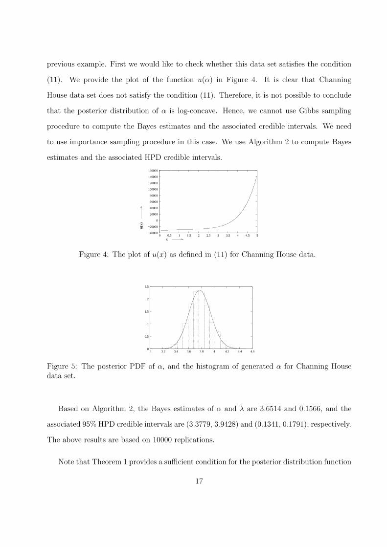
previous example. First we would like to check whether this data set satisfies the condition
(11). We provide the plot of the function u(α) in Figure 4. It is clear that Channing
House data set does not satisfy the condition (11). Therefore, it is not possible to conclude
that the posterior distribution of α is log-concave. Hence, we cannot use Gibbs sampling
procedure to compute the Bayes estimates and the associated credible intervals. We need
to use importance sampling procedure in this case. We use Algorithm 2 to compute Bayes
estimates and the associated HPD credible intervals.
x
u(x)
−40000
−20000
0
20000
40000
60000
80000
100000
120000
140000
160000
0 0.5 1 1.5 2 2.5 3 3.5 4 4.5 5
Figure 4: The plot of u(x) as defined in (11) for Channing House data.
0
0.5
1
1.5
2
2.5
3 3.2 3.4 3.6 3.8 4 4.2 4.4 4.6
Figure 5: The posterior PDF of α, and the histogram of generated α for Channing Housedata set.
Based on Algorithm 2, the Bayes estimates of α and λ are 3.6514 and 0.1566, and the
associated 95% HPD credible intervals are (3.3779, 3.9428) and (0.1341, 0.1791), respectively.
The above results are based on 10000 replications.
Note that Theorem 1 provides a sufficient condition for the posterior distribution function
17

0
5
10
15
20
25
30
0.1 0.12 0.14 0.16 0.18 0.2 0.22
Figure 6: The histogram of generated λ for Channing House data set.
of α to be log-concave. We would like to explore the posterior distribution function. We
plot the posterior PDF of α in Figure 5. It seems it can be approximated by a normal
distribution, which also has a log-concave PDF. Hence, in this case also Gibbs sampling
procedure can be used. We have generated α from the approximated normal distribution
and the corresponding histogram is also plotted along with PDF in the same figure. The
normal approximation works very well in this case. We have generated the corresponding λ
also as in Step 2 of Algorithm 1. The generated α has been plotted in Figure 6. Based on
the above normal approximation we obtain the Bayes estimates of α and λ as 3.7805 and
0.1451 respectively. The associated 95% HPD credible intervals become (3.4432, 4.1177) and
(0.1212, 0.1794), respectively. Gibbs sampling procedure is also based on 10000 replications.
5 Prediction Issues
5.1 Prediction for the Remaining Life
In this section, we develop a Bayesian prediction interval procedure to capture, with 100(1−
γ)% confidence, the future failure time of an individual item, conditioning on its survival
until its present age ti. The CDF for the lifetime of an item conditioning on its survival until
time ti is
F (t|ti, α, λ) = P (T ≤ t|T > ti, α, λ) = 1− e−λ(tα−tαi ); t > ti. (14)
18
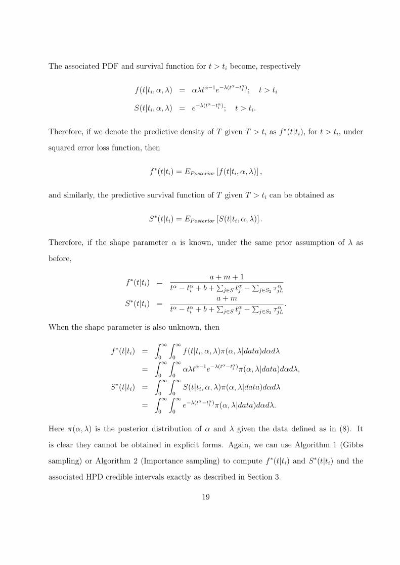
The associated PDF and survival function for t > ti become, respectively
f(t|ti, α, λ) = αλtα−1e−λ(tα−tαi ); t > ti
S(t|ti, α, λ) = e−λ(tα−tαi ); t > ti.
Therefore, if we denote the predictive density of T given T > ti as f∗(t|ti), for t > ti, under
squared error loss function, then
f ∗(t|ti) = EPosterior [f(t|ti, α, λ)] ,
and similarly, the predictive survival function of T given T > ti can be obtained as
S∗(t|ti) = EPosterior [S(t|ti, α, λ)] .
Therefore, if the shape parameter α is known, under the same prior assumption of λ as
before,
f ∗(t|ti) =a+m+ 1
tα − tαi + b+∑
j∈S tαj −
∑j∈S2
ταjL
S∗(t|ti) =a+m
tα − tαi + b+∑
j∈S tαj −
∑j∈S2
ταjL.
When the shape parameter is also unknown, then
f ∗(t|ti) =∫
∞
0
∫∞
0f(t|ti, α, λ)π(α, λ|data)dαdλ
=∫
∞
0
∫∞
0αλtα−1e−λ(tα−tαi )π(α, λ|data)dαdλ,
S∗(t|ti) =∫
∞
0
∫∞
0S(t|ti, α, λ)π(α, λ|data)dαdλ
=∫
∞
0
∫∞
0e−λ(tα−tαi )π(α, λ|data)dαdλ.
Here π(α, λ) is the posterior distribution of α and λ given the data defined as in (8). It
is clear they cannot be obtained in explicit forms. Again, we can use Algorithm 1 (Gibbs
sampling) or Algorithm 2 (Importance sampling) to compute f ∗(t|ti) and S∗(t|ti) and the
associated HPD credible intervals exactly as described in Section 3.
19

5.2 Prediction for the Cumulative Number of Failures in an
Interval
Suppose the i-th item belongs to S11∪S21, and ti denotes the censored time of the i-th item.
Further [L,R] is a fixed interval, and it is assumed that t∗ < L, where
t∗ = max{ti, i ∈ S11 ∪ S21}.
In this section we would like to predict the expected number of failures within the interval
[L,U ], out of n11 + n21 items which belong to S11 ∪ S21. The problem can be formulated as
follows. Let Zi be a Bernoulli random variable as follows:
Zi ={1 if i-th item fails within [L,R]0 otherwise,
(15)
and we want to compute
J =∑
i∈S11∪S21
E(Zi). (16)
It is immediate that for i ∈ S11 ∪ S21, then
E(Zi) = P (Zi = 1) = P (L < Ti ≤ U |T > ti) = S(L|ti, α, λ)− S(U |ti, α, λ)
= eλtαi
(e−λLα
− e−λUα).
Hence,
J =(e−λLα
− e−λUα) ∑
i∈S11∪S21
eλtαi .
Therefore, the Bayes estimate of J with respect to the squared error loss function and the
associated credible interval can be obtained along the same line as the method developed in
Section 3.
5.3 Channing House Data Revisited
In this section we reconsider the Channing house data set and first obtain the survival
probability till the time point t+ k for k > 0, given that the individual has survived till the
20

time point point t. We have used the same prior distributions and the same hyperparameters
as in Section 4. We report the Bayes estimates of the survival probabilities and the associated
95% HPD credible intervals for different k, namely k = 5, 10 and 15. The results are presented
in Table 5.
t t+ 5 t+ 10 t+ 15
60 0.998 0.978 0.904(0.997,0.999) (0.969, 0.985) (0.883, 0.924)
65 0.980 0.906 0.744(0.973, 0.986) (0.885, 0.925) (0.711,0.777)
70 0.924 0.759 0.513(0.910, 0.938) (0.731,0.789) (0.474,0.554)
75 0.822 0.555 0.288(0.801,0.842) (0.518,0.595) (0.238,0.332)
80 0.676 0.342 0.117(0.645,0.709) (0.294,0.395) (0.081,0.163)
Table 5: Probability that an individual will survive till the time point t+ k, given that theindividual has survived till the time point t.
One interesting point has come out from this table is that if a person has survived longer
then she/he has a more chance that she/he would live up to a certain age. For example
P (T > 80|T > 65) < P (T > 80|T > 70) or P (T > 90|T > 75) < P (T > 90|T > 80).
Moreover, for the same value of k, the length of the HPD credible intervals increase with t.
Finally, we compute the expected number of deaths among 286 survived ones and the
associated 95% HPD credible intervals for different age groups. The results are presented in
Table 6.
21

Age Group 70 - 75 75 - 80 80 - 90
J 21 46 140HPDCI (17,25) (42,51) (129, 151)
Table 6: The Bayes estimate of the expected number of failures (J) and the associated 95%HPD credible intervals (HPDCI) for different age-groups.
6 Conclusions
In this paper we consider the Bayesian inference of the Weibull parameters when the data
are left truncated and right censored. The usual maximum likelihood estimators may be
misleading, hence, Bayesian inference seems to be a natural choice. We have considered
fairly flexible priors on the scale and shape parameters, and propose to use Gibbs sampling
technique to compute Bayes estimates of the unknown parameters and the associated credible
intervals. Two data sets have been analyzed, and the performance of the proposed Bayes
estimators are quite satisfactory. We further address some prediction issues also, namely
the prediction for the remaining lifetime and prediction of the cumulative number of failures
during a specific interval. It will be of interest to consider the case when there are some
covariates also associated with each item/ individual. More work is needed along that
direction.
Acknowledgements:
The authors would like to thank two referees and the associate editor for their construc-
tive comments on the earlier draft of this manuscript, which has helped us to improve the
manuscript significantly.
22

Appendix
Proof of Theorem 1: We need to show that (10) is log-concave. Consider,
lnL(α|data) = k + ln π2(α) +m lnα + (α− 1)∑
i∈Sc
ln ti − (a+m) ln
b+
∑
i∈S
tαi −∑
i∈S2
ταiL
.
Suppose that g(α) = b+∑
i∈S
tαi −∑
i∈S2
ταiL, then
d
dαg(α) = g′(α) =
∑
i∈S
tαi ln ti −∑
i∈S2
ταiL ln τiL
d2
dα2g′(α) = g′′(α) =
∑
i∈S
tαi (ln ti)2 −
∑
i∈S2
ταiL(ln τiL)2.
Note that
g′′(α)g(α)− (g′(α))2 =∑
i,j∈A
(ln ti − ln tj)2 −
∑
i,j∈B
(ln ti − ln τjL)2 +
∑
i,j∈C
(ln τiL − ln τjL)2 ≥ 0.
Therefore, for b ≥ 0,d2
dα2ln π(α|data) ≤ 0. Hence, the result follows.
References
[1] Balakrishnan, N. and Mitra, D. (2011), “Likelihood inference for log-normal data
with left truncated and right censoring with an illustration”, Journal of Statistical
Planning and Inference vol. 141, 3536 - 3553.
[2] Balakrishnan, N. and Mitra, D. (2012), “Left truncated and right censored Weibull
data and likelihood inference with an illustration”, Computational Statistics and
Data Analysis vol. 56, 4011 - 4025.
[3] Balakrishnan, N. and Mitra, D. (2013), “Likelihood inference based on left trun-
cated and right censored gamma distribution”, IEEE Transactions on Reliability
vol. 62, 679 - 688.
23

[4] Balakrishnan, N. and Mitra, D. (2014), “Some further issues concerning likelihood
inference for left truncated and right censored log-normal data”, Communications
in Statistics - Simulation and Computation, vol. 43, 400 - 416.
[5] Berger, J.O. and Sun, D. (1993), “Bayesian analysis for Poly-Weibull distribution”,
Journal of the American Statistical Association, vol. 88, 1412 - 1418.
[6] Congdon, P. (2014), Applied Bayesian Modelling, 2nd edition, Wiley, New York.
[7] Devroye, L. (1984), “A simple algorithm for generating random variables with log-
concave density”, Computing, vol. 33, 247 - 257.
[8] Erto, P. (1980), “New practical Bayes estimators for the 2-parameter Weibull dis-
tribution”, IEEE Transactions on Reliability Analysis, vol. 31, 194 - 197.
[9] Geman, S. and Geman, A. (1984), “Stochastic relaxation, Gibbs distribution and
the Bayesian reconstruction of images”, IEEE Transactions on Pattern Analysis
and Machine Intelligence, vol. 6, 721 - 740.
[10] Hamada, M.S., Wilson, A., Reese, C.S. and Martz, H. (2008), Bayesian Reliability,
Springer Science & Business Media, New York.
[11] Hong, Y., Meeker, W.Q. and McCalley, J.D. (2009), “Prediction of remaining life
of power transformers based on left truncated and right censored lifetime data”,
The Annals of Applied Statistics, vol. 3, 857 - 879.
[12] Kaminskiy, M.P. and Krivtson, V.V. (1995), “A simple procedure for Bayesian
estimation of the Weibull distribution”, IEEE Transactions on Reliability Analysis,
vol. 54, 612 - 616.
[13] Kundu, D. (2008), “Bayesian inference and life testing plan for Weibull distribution
in presence of progressive censoring”, Technometrics, vol. 50, 144 - 154.
24

[14] Pradhan, B. and Kundu, D. (2014), “Analysis of interval-censored data with
Weibull lifetime distribution”, Sankhya B, vol. 76, 120 - 139.
25

Appendix B: Data
S.N. Year of Year of ν δ S.N. Year of Year of ν δ S.N. Year of Year of ν δ
Inst. Exit Inst. Exit Inst. Exit
1 1961 1996 0 1 11 1963 2008 0 0 21 1960 1988 0 1
2 1964 1985 0 1 12 1963 2000 0 1 22 1961 1993 0 1
3 1962 2007 0 1 13 1960 1981 0 1 23 1961 1990 0 1
4 1962 1986 0 1 14 1963 1984 0 1 24 1960 1986 0 1
5 1961 1992 0 1 15 1963 1993 0 1 25 1962 2008 0 0
6 1962 1987 0 1 16 1964 1992 0 1 26 1964 1982 0 1
7 1964 1993 0 1 17 1961 1981 0 1 27 1963 1984 0 1
8 1960 1984 0 1 18 1960 1995 0 1 28 1960 1987 0 1
9 1963 1997 0 1 19 1961 2008 0 0 29 1962 1996 0 1
10 1962 1995 0 1 20 1960 2002 0 1 30 1963 1994 0 1
31 1987 2008 1 0 41 1980 2008 1 0 51 1984 2001 1 1
32 1980 2008 1 0 42 1982 2008 1 0 52 1983 2008 1 0
33 1988 2008 1 0 43 1986 2008 1 0 53 1988 2008 1 0
34 1985 2008 1 0 44 1984 2008 1 0 54 1988 2008 1 0
35 1989 2008 1 0 45 1986 1995 1 1 55 1985 2008 1 0
36 1981 2008 1 0 46 1986 2008 1 0 56 1986 2008 1 0
37 1985 2008 1 0 47 1987 2008 1 0 57 1988 2008 1 0
38 1986 2004 1 1 48 1986 2008 1 0 58 1982 2008 1 0
39 1980 1987 1 1 49 1986 2008 1 0 59 1985 2008 1 0
40 1986 2005 1 1 50 1984 2008 1 0 60 1988 2008 1 0
61 1982 2004 1 1 71 1989 2008 1 0 81 1981 2006 1 1
62 1980 2008 1 0 72 1989 2008 1 0 82 1988 1996 1 1
63 1980 2002 1 1 73 1986 2008 1 0 83 1985 2002 1 1
64 1984 2008 1 0 74 1982 1999 1 1 84 1984 2008 1 0
65 1981 1999 1 1 75 1985 2008 1 0 85 1980 2008 1 0
66 1986 2007 1 1 76 1986 2008 1 0 86 1982 2008 1 0
67 1987 2008 1 0 77 1982 2008 1 0 87 1981 1995 1 1
68 1983 2008 1 0 78 1988 2004 1 1 88 1986 1997 1 1
69 1983 2006 1 1 79 1980 2008 1 0 89 1986 2008 1 0
70 1983 1993 1 1 80 1982 2002 1 1 90 1986 2008 1 0
91 1982 2008 1 0 96 1986 2008 1 0
92 1989 2008 1 0 97 1982 1996 1 1
93 1984 2008 1 0 98 1982 2008 1 0
94 1980 2008 1 0 99 1982 2008 1 0
95 1988 2008 1 0 100 1989 2008 1 0
Table 7: Simulated year of installation, year of exit of the transformers along with thetruncation and censoring indicators.
26
Recommended


![Bayesian Inference for Weibull distribution Under The ...home.iitk.ac.in/~kundu/bayesian_weibull_bjpc.pdfCohen [5], [6] described the importance of the progressive cen-soring scheme](https://img.dokumen.tips/doc/110x75/60ebffb20de43b430d734f23/bayesian-inference-for-weibull-distribution-under-the-homeiitkacinkundubayesianweibullbjpcpdf.jpg)