Bayesian Forecasting of Stock Prices
Via the Ohlson ModelBy
Qunfang Flora LuA Thesis
Submitted to the Faculty
of
WORCESTER POLYTECHNIC INSTITUTE
in partial fulfillment of the requirements for the
Degree of Master of Science
in
Applied Statistics
by
May 2005
APPROVED:
Balgobin Nandram, Professor and major advisor
Huong Higgins, Associate Professor and co-advisor
Bogdan Vernescu, Professor and Department Head
1

Abstract
Over the past decade of accounting and finance research, the Ohlson (1995) model has
been widely adopted as a framework for stock price prediction. While using the
accounting data of 391 companies from SP500 in this paper, Bayesian statistical
techniques are adopted to enhance both the estimative and predictive qualities of the
Ohlson model comparing to the classical approaches. Specifically, the classical methods
are used for the exploratory data analysis and then the Bayesian strategies are applied
using Markov chain Monte Carlo method in three stages: individual analysis for each
company, grouping analysis for each group and adaptive analysis by pooling information
across companies. The base data, which consist of 20 quarters’ observations starting
from the first quarter of 1998, are used to make inferences for the regression coefficients
(or parameters), evaluate the model adequacy and predict the stock price for the first
quarter of 2004, when the real observations are set as the test data to evaluate the
predictive ability of the Ohlson model. The results are averaged within each specified
group categorized via the general industrial classification (GIC). The empirical results
show that classical models result in larger stock price prediction errors, more positively-
biased predictions and have much smaller explanatory powers than Bayesian models. A
few transformations of both classical and Bayesian models are also performed in this
paper, however, transformations of the classical models do not outweigh the usefulness of
applying Bayesian statistics.
2

Acknowledgements
I would like to express my deep gratitude to the following people for their academic,
financial or spiritual support in finishing this thesis.
Advisors: Balgobin Nandram and Huong Higgins. Without their help and guidance, there
would not have been such a piece of work. There are no words that can express the
appreciation from the bottom of my heart to them. And I promise this is not the end of
my devotion to the research on this topic. I will keep in touch with them wherever I am.
Professors in the Math Department of WPI: Joseph D. Petruccelli, Jayson Wilbur,
Andrew Swift, Carlos Morales and Christopher J. Larsen. Their courses have
strengthened my knowledge in Applied Statistics and Applied Math. Also thank to
Mayer Humi, William W. Farr, John Goulet, Dalin Tang, Peter R. Christopher and
William J. Martin for their guidance in my two years of working experience as a teaching
assistant.
Secretaries in the Math Department of WPI: Colleen Lewis, Ellen Mackin, Deborah Riel.
They are the nicest, most patient and helpful secretaries that I’ve ever seen. Best wishes
to them forever!
My parents and brother: Zhongxiao Lu, Rongzhi Liu, Hanliang Lu. They are always there
when I’m in need; they accept me when I’m rejected; they are still proud of me even
when I do not feel any good about a single part of myself.
My fiancé and his family: John Cacka, Bethlynne Vanella and Jennifer Graham etc. They
gave me a warm home when I was in the hardest time in USA, and have been supporting
me even since then. They like Chinese, I love them.
WPI Ballroom Dance Team: Boris Mosis and Miles Schofield etc. They helped me
develop a terrific hobby --- dancing, which is my life, my soul and my best joy in the free
time. Thanks for all those exciting practice lessons and dance parties.
3

Colleagues and classmates: Fang Huang, Yan Bai, Guochun Liu, Alina Ursan, Shinji
Uemura, Gregory Matthews, Shawn Hallinan, Ashley Moraski, Rajesh Kondapaneni,
Jasraj Kohli, Daniel Onofrei, Bijaya Padhy, Elizabeth Teixeira and Scott Laine etc. I had
fun discussing homework problems with them. Sometimes we also talked about life,
worries and future dreams. They are nice, smart and very friendly. I will keep them in
my memory.
Friends: Jeani Lu, Mark Bertolina, Alin Sirbu, Congmei Ma, Chi Hu, Pong Pang, Fang
Liu, Yucong Huang, Qunwei Ai, Chao Ku and Xiaolin Nan etc. They are not many, but
enough to make me a rich and confident woman.
Last but not least, to those who doubt my intelligence, willpower and potential. I will fan
the flame of dissatisfaction and make a miracle to them, to myself and to this wonderful
world.
4

Chapter 1
The Ohlson (1995) Model and Data of S&P 500
1.1 The Ohlson (1995) Model
Over the past two decades in finance and accounting area, considerable attention has been
paid to the relationship between accounting numbers (book values, earnings, etc.) and the
firm value. The Ohlson (1995) approach to the problem of stock valuation relates
securities prices to accounting data, and provides a structure for applicable modeling.
The Ohlson (1995) Valuation Model has been widely adopted by researchers and
practitioners on profitability analysis as a framework for the fundamental valuation of
equities. It also has been developed into several versions, e.g., Feltham-Ohlson (1995)
Valuation Model, Bernard’s (1995) Ohlson Approximation Model, Liu-Ohlson (2000)
Valuation Model and Callen’s (2001) Ohlson AR(2) Valuation Model. For a historical
development process of the Ohlson model, see Appendix A.
This paper evaluates the Ohlson (1995) Forecasting Model (OFM), or briefly the Ohlson
(1995) model, and uses it to forecast stock prices. OFM is a practicable case of Bernard’s
(1995) Ohlson Approximation Model (see Appendix C). For a single firm, OFM states:
the stock price per share is a linear function of the company’s book value per share and
abnormal earnings per share for the following four periods with normally distributed
innovation terms, which represents “other information” whose source is uncorrelated with
abnormal earnings. In mathematical form, it can be expressed as
, , ,1 ,4321
,~
'
~
4
1221
Tt, , , k
vxvxbvy tt
tk
aktktt
==
+=+++= ∑=
++ ββββ (1.1.1)
where ty denotes the stock price per share at time t, tbv is the book value per share at
time t, atx represents the abnormal earning at time t, )',( 61
~βββ = is the vector of
5

intercept and slope coefficients of the predictors, )',,,,,1( 4321'
~
at
at
at
att
txxxxbvx ++++= is the
vector of intercept and predictors, and tv is the innovation (error or residual) term.
To understand the “abnormal earning” term, we can view it as a contraction of “above
normal earning”. Ohlson (1995) proposes the abnormal earning as
,1−−= tttat bvrxx (1.1.2)
where tx is the earning per share at time t for a company, tr is the discount rate at time t.
Since the values of the following four periods ( ),,, 4321at
at
at
at xxxx ++++ are used to forecast the
stock price, this paper uses the expected earnings to replace tx in (1.1.2). That is,
1][ −−= tttat bvrxEx . (1.1.3)
For the innovation term, Ohlson (1995) assumes it has a first order autoregressive
structure (AR(1)). This assumption can be described as
),,0(~
,2
1
σε
ερ
Nvv
t
ttt += − (1.1.4)
where ρ is the correlation coefficient of time series tv , tε is the white noise, 2σ is the
variance of the white noise. Note that if 1<ρ , the AR(1) process is stationary.
From (1.1.1) and (1.1.4) we can get
,~
'
1~11 β−
−− −=t
tt xyv
.
,
~
'
1~1~
'
~
~
'
1~11
ttttt
tt
tttt
xyxy
xyvv
εβρβ
εβρερ
+
−+=
+
−=+=
−−
−−−
6
But when 1=t , 1~
'
0~0
~
'
1~1 εβρβ +
−+= xyxy , there exists unobserved values 0y and
'
0~x .
This paper lets
−=~
'
0~0 βρµ xy . Therefore, expressions (1.1.1) and (1.1.4) can be
combined as
, , ,1 ), ,0(~
, , ,2 ,)(
,
2
~
'11
~
'
1~
'11
TtN
Ttxyxy
xy
iid
t
ttttt
=
=+−+=
++=
−−
σε
εβρβ
εµβ
(1.1.5)
where µ , ρ and 2σ are three unknown parameters besides the intercept and regression
coefficients in ~β .
Expression (1.1.5) is the complete form of the Ohlson (1995) Forecasting Model,
hereinafter the Ohlson model, that is used in this paper.
1.2 Retrieving Data of S&P 500 from Thomson ONE Analytics
Yearly or quarterly data from various sources have been applied to test the Ohlson model.
For instances, besides many tests that use US data, Bao & Chow (1999) test the
usefulness of the Ohlson model using data from listed companies in the People’s
Republic of China; McCrave & Nilsson (2001) compare the difference between Swedish
and US firms by using data from a Swedish business magazine, Bonnier-Findata database
and I/B/E/S database; Ota (2002) uses empirical evidence from Japan, etc. This paper
applies quarterly data of S&P 500 from Thosmon ONE Analytics to the Ohlson model.
S&P 500 is one of the most widely used measures of U.S. stock market performance and
is considered to be a bellwether for the U.S. economy. S&P refers to Standard & Poor’s,
which is a division of the McGraw-Hill Companies, Inc. 500 companies are selected
among the leaders in the major industries driving U.S. economy by the S&P Index
7

Committee for market size, liquidity and sector representation. A small number of
international companies that are widely traded in the U.S are included.
The needed data of S&P 500 can be retrieved from Thomson ONE Analytics by its Excel
Add-in software, provided by the Thomson Corporation, which is a global leader in
providing value-added information, software applications and tools in the fields of law,
tax, accounting, financial services and corporate training and assessment etc. Thomson
ONE Analytics is a web based application that allows users to research information about
different companies and markets, including current stock prices, volume traded, EPS
(expected earning per share) and so on. The “Thomson ONE Analytics Excel Add-in” is
one of the most valuable features that Thomson ONE Analytics offers its users. Using
the Add-in, financial analysts can pull data directly into Excel from a wealth of financial
databases such as “Worldscope”, “Compustat”, “U.S. Pricing”, “I/B/E/S and I/B/E/S
History” and “Extel” by using the powerful PFDL (Premier Financial Database
Language).
Items in the retrieved data are: Total Assets, Total Liabilities, Preferred Stock, Common
Shares Outstanding from database “Worldscope”; “EPSmeanQTR1-4” and
“EPSConsensusForecastPeriodQTR1-4” from database “I/B/E/S History” (note that these
are monthly data); Dow Jones Industry Group (DJIC), General Industry Classification
(GIC), Dow Jones Market Sector (DJMS) and GICSSECTOR from “Thomson
Financial”; PriceClose and 3-month T-bill (treasury bill) rate from “Datastream”. Book
value per common share (BPS) can be calculated by the first four items in following
formula:
BPS = (Total Assets − Total Liabilities − Preferred Stock)/(Common Shares
Outstanding).
Companies forecast their expected earnings every month for the following four fiscal
quarters. This paper uses the latest forecast value for each quarter to represent the
corresponding quarter value. The quarterly EPS are extracted from the monthly data of
“EPSmeanQTR1-4” and “EPSConsensusForecastPeriodQTR1-4”. For easier use, values
8

of Dow Jones Industry Group, Dow Jones Market Sector and the Company Identity Keys
are transformed into integers. (For example, use 3104 instead of the original value
C000003104.) To understand these financial / accounting terms, please see Appendix D.
Appendix E explains how to use Excel Add-in. Appendix F explains how to extract
quarterly data out of monthly data.
After deleting all the missing and incomplete data points and the data points that cause
programming errors, 391 companies are selected. This final quarterly data set have 21
points for each company, covering 25 quarters from the first quarter of 1998 and the first
quarter of 2004. It is formatted into 16 items which are all numerical values and contain
4 sectors (DJIC, GIC, DJMS and GICSSECTOR), company identity key (ID), Time,
PriceClose, BPCS0-3, EPS1-4 and R (3-month T-bill rate).
1.3 Exploratory Data Analysis by Classical Approaches
While considering the ideas in various versions of the Ohlson model, this paper sticks to
the main frame of the Ohlson model in (1.1.5), and sets up 11 different models which are
described in Table 1.3.1 for the exploratory analysis.
These 11 models can be classified into three groups by distinguishing the assumption of
the innovation term: independent errors among time periods which belongs to the
ordinary linear regression structure (OLR), AR(1) structure for the error and AR(2)
structure for the error. The main point of this classification is to check whether the AR(1)
assumption is proper for the innovation term of the Ohlson model. Besides this, four
kinds of transformation to the term of stock price per share are applied to the model under
either AR(1) or AR(2) assumption for the innovation term: logarithmic transformation
(log trans), square root transformation (sqrt trans), cubic root transformation (curt trans)
and inverse transformation (inv trans). Two relatively better transformations are to be
selected by the classical statistical analysis. This paper assumes their priorities to be
adopted in further research by the innovative methods, for the reason of their being more
fit to the data. The purpose of using transformations is to improve both the estimative
9

and predictive qualities of the Ohlson model.
Table 1.3.1 --- Various Models
Name Equation
OFM --- OLR ),0(~, 24
1110 σεεβββ Nxbvy
iid
tta
ktk
ktt +++= +=
+∑
OFM --- AR(1) ),0(~,, 21
4
1110 σεερβββ Nvvvxbvy
iid
ttttta
ktk
ktt +=+++= −+=
+∑
OFM --- AR(2) ),0(~,, 22211
4
1110 σεερρβββ Nvvvvxbvy
iid
tttttta
ktk
ktt ++=+++= −−+=
+∑log trans of OFM AR(1) ),0(~,,)log( 2
1
4
1110 σεερβββ Nvvvxbvy
iid
ttttta
ktk
ktt +=+++= −+=
+∑sqrt trans of
OFM --- AR(1) ),0(~,, 21
4
1110 σεερβββ Nvvvxbvy
iid
ttttta
ktk
ktt +=+++= −+=
+∑ curt trans of
OFM --- AR(1) ),0(~,, 21
4
1110
3 σεερβββ Nvvvxbvyiid
ttttta
ktk
ktt +=+++= −+=
+∑inv trans of
OFM --- AR(1) ),0(~,,/1 21
4
1110 σεερβββ Nvvvxbvy
iid
ttttta
ktk
ktt +=+++= −+=
+∑log trans of OFM AR(2) ),0(~,,)log( 2
2211
4
1110 σεερρβββ Nvvvvxbvy
iid
tttttta
ktk
ktt ++=+++= −−+=
+∑sqrt trans of
OFM --- AR(2) ),0(~,, 22211
4
1110 σεερρβββ Nvvvvxbvy
iid
tttttta
ktk
ktt ++=+++= −−+=
+∑ curt trans of
OFM --- AR(2) ),0(~,, 22211
4
1110
3 σεερρβββ Nvvvvxbvyiid
tttttta
ktk
ktt ++=+++= −−+=
+∑inv trans of
OFM --- AR(2) ),0(~,,/1 22211
4
1110 σεερρβββ Nvvvvxbvy
iid
tttttta
ktk
ktt ++=+++= −−+=
+∑
Two procedures, PROC REG and PROC AUTOREG in SAS, are the classical methods
that are used to the whole data set to test the estimative ability of the 11 models.
Specifically, PROC REG is only used to model OFM---OLR and PROC AUTOREG is
used to the models with AR(p) structures for the innovation term. Three kinds of criteria
are used to compare their estimative abilities: R-squares (total R-square and Regress R-
square), Akaike Information Criterion (AIC) and Bayesian Information Criterion (BIC).
See Table 1.3.2 for the empirical results. Note that R-square is the coefficient of
determination (regression sum of squares divided by total sum of squares). Total R-
square is R-square and regress R-square is R-square adjusted for additional covariates.
They are nearly the same in PROC REG procedure, but can be very different in PROC
AUTOREG procedure, especially when the innovation terms are highly correlated among
10
time periods. BIC is a quantity proportional to the negative log likelihood after all
parameters are integrated out. AIC is a deviance measure (i.e., difference between
observed and fitted models). Models with small AIC and BIC values are preferred.
Table 1.3.2 --- Overall Estimative Ability Comparison of Various Models
Model Total R-square
Regress R-square AIC BIC
OFM --- OLR 0.2184 0.2184OFM --- AR(1) 0.7526 0.0856 59112 59161OFM --- AR(2) 0.7526 0.0857 59114 59170
log trans of OFM AR(1) 0.7680 0.1033 2653 2702 sqrt trans of OFM --- AR(1) 0.7716 0.1016 18013 18062curt trans of OFM --- AR(1) 0.7733 0.1046 2026 2076 inv trans of OFM --- AR(1) 0.6230 0.0413 -35734 -35685
log trans of OFM AR(2) 0.7680 0.1034 2656 2712sqrt trans of OFM --- AR(2) 0.7716 0.1021 18016 18072curt trans of OFM --- AR(2) 0.7733 0.1048 2030 2086inv trans of OFM --- AR(2) 0.6242 0.0413 -35756 -35701
The following conclusions can be drawn by comparing the R-squares, AIC’s and BIC’s in
Table 1.3.2.
• Using PROC REG to model OFM---OLR, R-square turns out to be very small
(0.2184). Using PROC AUTOREG to the other 10 models, the Total R-square
values are over 0.75 to all except in the cases of using inverse transformation. For
the models with AR(p) structure to the innovation term, the results show big
difference between the Total R-square (>0.75) and the Regress R-square (<0.11).
All these results indicate that the assumption of independence of the innovation
terms among different time periods cannot stand. In other words, setting an AR
(p) structure to the innovation term can be a sound assumption.
• AR(2) structure is no better than AR(1), for they have extremely close R-square
values. This is in line with the conclusion drawn by Callen (2001).
• The Total R-square value (0.6230) under the inverse transformation is much less
than without a transformation (0.7526), while the Total R-square values under the
other three transformations are slightly bigger than without a transformation. This
concludes that the inverse transformation cannot enhance the estimative ability,
while the other three can slightly enhance the estimative ability.
11

• Based on Total R-square value, cubic root transformation enhances the estimative
ability the most (0.7733), then the square root transformation (0.7716), and then
the log transformation (0.7680). But the differences among them are very small.
Based on AIC and BIC, cubic transformation has the smallest value (2026 and
2076), then the log transformation (2653 and 2702). The square root
transformation has much larger AIC and BIC (18013 and 18062). Therefore,
cubic root transformation and log transformation are relative better than the
others.
After comparing the estimative abilities of the 11 models, this paper proceeds further
exploratory analysis by concentrating on 3 models: OFM --- AR(1), log trans of
OFM AR(1) and curt trans of OFM --- AR(1).
In order to test the predictive abilities of the models, the retrieved data of S&P 500 are
divided into two parts for each company. The first part contains the first 20 periods of
data which will be used as base data to estimate regression coefficients; the second part
has the 21st period of data which will be used as test data to compare with the predictions
for this period from the base data. (The same base data and test data as in this division are
also used in the following chapters.)
After using PROC AUTOREG to the data in each GIC group (see Table 1.3.3 for the
General Industrial Classification Distribution), the estimated regression coefficients for
three models are collected in Table 1.3.4. The results show that the intercept, BPS and
abnormal earnings per share of the first two following quarters are generally significant in
the Ohlson Model. (The values in bold are significant, others are insignificant.)
Table 1.3.3 --- General Industrial Classification (GIC) Distribution
GIC Value 0 1 2 3 4 5 6
Class Overall Industrial Utility Transportation Banks/Savings and Loan Insurance Other
FinancialNo. of Firms 391 284 42 5 29 18 13
Note: when GIC equals 0, it means this group includes all 391 firms.
12
The PROC AUTOREG procedure also gives the predicted values of the 21st period using
the base data. To compare the predictive abilities among the three selected models for
different GIC groups, the criterion is defined as
212121 /)ˆ( yyyR −= (1.3.1)
where R is the relative difference of predicted stock price over real stock price for a
company, 21y is the predicted stock price of a company for the 21st period, 21y is the real
stock price of a company for the 21st period.
Table 1.3.4 --- Estimated Parameters from Base DataGIC = 0
Model Beta1 Beta2 Beta3 Beta4 Beta5 Beta6OFM --- AR(1) 25.7102 0.8006 4.4180 3.4307 -0.089 0.0456
LOG-trans of OFM AR(1) 3.075 0.0288 0.1492 0.1047 0.006134 -0.0111CURT-trans of OFM --- AR(1) 2.8435 0.0279 0.1471 0.1076 0.003040 -0.007624
GIC = 1Model Beta1 Beta2 Beta3 Beta4 Beta5 Beta6
OFM --- AR(1) 25.2903 0.8929 6.1202 5.5564 0.2602 0.1988LOG-trans of OFM AR(1) 3.0464 0.0329 0.2143 0.1678 0.0279 -0.002011
CURT-trans of OFM --- AR(1) 2.8201 0.0317 0.2094 0.1742 0.0214 0.000176GIC = 2
Model Beta1 Beta2 Beta3 Beta4 Beta5 Beta6OFM --- AR(1) 23.0625 0.6416 1.7959 -0.3845 0.4846 0.2983
LOG-trans of OFM AR(1) 2.9159 0.0290 0.0645 0.000787 0.000355 -0.0129
CURT-trans of OFM --- AR(1) 2.7138 0.0262 0.0608 -0.005617 0.006043 -0.008238
GIC = 3Model Beta1 Beta2 Beta3 Beta4 Beta5 Beta6
OFM --- AR(1) 11.2044 0.9892 3.4738 1.4118 1.0681 -1.3959LOG-trans of OFM AR(1) 2.6101 0.0342 0.1238 0.0204 0.0220 -0.0415
CURT-trans of OFM --- AR(1) 2.3632 0.0343 0.1218 0.0292 0.0265 -0.0442GIC = 4
Model Beta1 Beta2 Beta3 Beta4 Beta5 Beta6OFM --- AR(1) 18.6728 1.3250 8.7575 -4.6200 -7.4562 0.7041
LOG-trans of OFM AR(1) 3.0660 0.0316 0.2109 -0.0500 -0.1922 -0.0129CURT-trans of OFM --- AR(1) 2.7515 0.0361 0.2419 -0.0800 -0.2187 -0.002449
GIC = 5Model Beta1 Beta2 Beta3 Beta4 Beta5 Beta6
OFM --- AR(1) 31.9752 0.6065 -3.0127 1.7879 -1.2500 0.0256LOG-trans of OFM AR(1) 3.4200 0.0147 -0.0591 0.0356 -0.0168 -0.008506
CURT-trans of OFM --- AR(1) 3.1393 0.0166 -0.0739 0.0450 -0.0241 -0.006542GIC = 6
Model Beta1 Beta2 Beta3 Beta4 Beta5 Beta6OFM --- AR(1) 30.5121 0.6323 15.9995 5.2249 -6.2083 -1.3595
LOG-trans of OFM AR(1) 3.2711 0.0194 0.4457 0.1451 -0.1619 -0.0580CURT-trans of OFM --- AR(1) 3.0281 0.0199 0.4742 0.1528 0.1816 -0.0536
13
The following conclusions can be drawn from Table 1.3.5 where the quantiles of R , the
number of nonnegative R ’s (No.(+,0)) and the number of negative R ’s (No. (-)) are
collected. The digital “1” and “2” after the names of transformations are to distinguish
different scales of measurement. “1” denotes using the original scale, “2” denotes using
the transformed scale.
Table 1.3.5 --- Quantiles of R and Number of Nonnegative/Negative R’s
(1 --- Original Scale 2 --- Transformed Scale)
GIC No. ofFirms Model Min Q1 Q2 Q3 Max No.
(+,0)No.(-)
0 391
OFM --- AR(1) -0.490 0.073 0.400 0.936 15.703 315 76log trans of OFM AR(1)-1 -0.564 -0.038 0.347 0.795 13.137 284 107log trans of OFM AR(1)-2 -0.196 -0.010 0.088 0.191 6.875 284 107curt trans of OFM AR(1)-1 -0.540 -0.004 0.360 0.804 13.992 292 99curt trans of OFM AR(1)-2 -0.227 0.000 0.109 0.219 1.466 293 98
1 284
OFM --- AR(1) -0.458 0.058 0.440 1.059 15.277 225 59log trans of OFM AR(1)-1 -0.531 -0.029 0.365 0.879 12.626 208 76log trans of OFM AR(1)-2 -0.179 -0.008 0.098 0.214 6.780 208 76curt trans of OFM AR(1)-1 -0.507 -0.013 0.416 0.899 13.496 210 74curt trans of OFM AR(1)-2 -0.209 -0.003 0.124 0.240 1.439 210 74
2 42
OFM --- AR(1) -0.197 0.068 0.281 1.411 9.235 35 7log trans of OFM AR(1)-1 -0.340 0.000 0.174 1.062 7.412 31 11log trans of OFM AR(1)-2 0.120 0.000 0.049 0.284 2.220 31 11curt trans of OFM AR(1)-1 -0.284 0.014 0.208 1.185 8.042 33 9curt trans of OFM AR(1)-2 -0.104 0.006 0.066 0.299 1.084 34 8
3 5
OFM --- AR(1) 0.041 0.195 0.359 0.474 0.574 5 0log trans of OFM AR(1)-1 0.162 0.180 0.181 0.357 0.368 5 0log trans of OFM AR(1)-2 0.042 0.052 0.056 0.093 0.105 5 0curt trans of OFM AR(1)-1 0.111 0.180 0.242 0.407 0.430 5 0curt trans of OFM AR(1)-2 0.037 0.058 0.076 0.122 0.128 5 0
4 29
OFM --- AR(1) -0.251 0.171 0.306 0.480 1.394 25 4log trans of OFM AR(1)-1 -0.323 0.054 0.185 0.402 1.194 24 5log trans of OFM AR(1)-2 -0.100 0.015 0.051 0.113 0.299 24 5curt trans of OFM AR(1)-1 -0.302 0.089 0.220 0.424 1.252 24 5curt trans of OFM AR(1)-2 -0.112 0.030 0.070 0.126 0.312 24 5
5 18
OFM --- AR(1) -0.313 0.120 0.242 0.390 3.663 15 3log trans of OFM AR(1)-1 -0.359 0.047 0.190 0.302 3.357 14 4log trans of OFM AR(1)-2 -0.109 0.013 0.047 0.076 0.645 14 4curt trans of OFM AR(1)-1 -0.347 0.066 0.197 0.324 3.435 14 4curt trans of OFM AR(1)-2 0.131 0.023 0.063 0.099 0.644 14 4
6 13
OFM --- AR(1) -0.045 0.195 0.348 0.847 4.276 12 1log trans of OFM AR(1)-1 -0.105 0.143 0.266 0.810 3.562 11 2log trans of OFM AR(1)-2 -0.031 0.037 0.071 0.174 0.807 11 2curt trans of OFM AR(1)-1 0.075 0.370 0.466 1.266 4.128 13 0curt trans of OFM AR(1)-2 0.026 0.112 0.138 0.315 0.726 13 0
14

The empirical results show that the distributions of R are asymmetrical with long tails,
which suggests the 50% quantile (Q2) of R as a major criterion. From Table 1.3.5, the
following conclusions can be drawn.
• Based on Q2 values in original scale, the ratio value ranges from 24.2% (GIC = 5)
to 44% (GIC = 1) and 40% overall (GIC = 0) under no transformation, from
17.4% (GIC = 2) to 36.5% (GIC = 1) and 34.7% overall (GIC = 0) under log
transformation, and from 19.7% (GIC = 5) to 46.6% (GIC = 6) and 36% overall
(GIC = 0) under cubic root transformation. Based on Q2 values in transformed
scale, the ratio value ranges from 4.7% (GIC = 5) to 9.8% (GIC = 1) and 8.8%
overall (GIC = 0) under log transformation, and from 6.3% (GIC = 5) to 13.8%
(GIC = 6) and 10.9% overall (GIC = 0) under cubic root transformation. These
conclude that the log transformation improves the predictive ability more than the
cubic root transformation does while using the classical method.
• In all cases, the number nonnegative R ’s is much larger than the number of
negative R ’s, which shows the high overestimation by the classical method.
The too large magnitude of R and the extremely high overestimation state that using the
classical method (the PROC AUTOREG procedure) to interpret the Ohlson model is not
efficient enough in forecasting stock prices. A better approach is desired to improve both
the estimative and predictive abilities of the Ohlson model.
Summarily, the exploratory data analysis by PROC REG/AUTOREG confirms the AR(1)
assumption of the innovation term in the Ohlson model, and the promising effect of
adopting logarithmic transformation as well as cubic root transformation. It suggests that
the remaining work focus on 3 models: OFM --- AR(1), log trans of OFM AR(1) and curt
trans of OFM --- AR(1). Since the Ohlson model is not able to predict the stock price
efficiently by the classical means, this paper applies an innovative statistical method,
Bayesian statistical analysis, to the 3 chosen models in the remaining work.
1.4 An Outline of Bayesian Statistical Analysis
In the following three chapters of this paper, Bayesian approaches are used for the
purpose of satisfying the requirement of improving both the estimative and predictive
15

qualities of the Ohlson model, comparing to the classical methods. In detail, Chapter 2
uses the most basic Bayesian techniques to each company, which is the case that different
companies have different regression coefficients; Chapter 3 applies the Bayesian method
by letting all the companies in each group share the same regression coefficients. While
Chapter 2 represents the individual analysis, Chapter 3 represents the grouping analysis.
And Chapter 4 ends up to be the adaptive analysis by pooling information across
companies. That is, different companies have different regression coefficients in Chapter
4, and in the mean time they are pooled together. Basically, Chapter 4 compromises the
ideas in Chapter 2 and the ones in Chapter 3.
For each Bayesian approach in following three chapters, the main tasks are to make
inferences for the regression coefficients (or parameters), evaluate the model adequacy
and test the predictive ability of the Ohlson model. Chapter 5 concludes all the work in
this paper, which includes the comparison among the three Bayesian approaches as well
as the comparison of the best Bayesian approach to the classical method.
16

Chapter 2
Bayesian Statistical Analysis for Individual Firm
2.1 Bayesian Version of the Ohlson Model for a Single Firm
As an extreme case, this chapter assumes all the companies are independent of each other
and have their own regression coefficients in the Ohlson model. At the very beginning of
applying the Bayesian statistical analysis to each company, a Bayesian version of the
Ohlson model is set up in the following three steps.
First, for a specific company, describe the observation ),,,( 21~
Tyyyy = by the
parameters ,,, 2
~σρµβ . Under the assumption that the observations are conditionally
independent among the time periods, we can get the likelihood function from expression
(1.1.5):
∏= −
−
−+⋅+=T
t tttt xyxyNxyNyp2
2
~
'
1~1~
'
~
2
~
'
1~12
~~),|(),|(),,,|( σβρβσµβσρµβ .
(2.1.1)
Second, assign a prior distribution to each unknown parameter. The prior distribution
represents a population of possible parameter values, from which the parameter of current
interest has been drawn. The guiding principle is to express the knowledge (and
uncertainty) about the parameter as if its value could be thought of as a random
realization from the prior distribution. In order to get the practical advantage of being
interpretable as additional data and computational convenience, this paper assigns the
conjugate prior distributions as follows:
).,|()(),1,1|()(
),,|()(
),,|()(
22
200
00~~~
baIUN
NK
σσπ
ρρπσµµµπ
θββπ
Γ=
−==
∆=
(2.1.2)
17
The hyperparameters ,,, 2000
0~σµθ ∆ in (2.1.2) are set as follows.
(P2.1) ~
1
0~')'( yXXXB −==θ .
The idea of setting 0~
θ is to use the estimation of~β in the ordinary linear
regression model
, , ,1 ),,0(~ , 2
~
' TtNxyiid
tttt =+= σεεβ (OLM-1)
by the method of least squares. Note that ( )'
~
'
2~
'
1~,,,
TxxxX = is the matrix of all
covariates together with an intercept, )',,,,,1( 4321'
~
at
at
at
att
txxxxbvx ++++= ( Tt , ,1 = )
is the regression coefficient vector consisting of the 1 and predictors, andT is the
number of time periods.
(P2.2) PT
SSXX E
−=∆ −1
0 )'(100 , where yXByySSE ''' −= is the sum of squares of the
errors of (OLM-1), P is the number of regression coefficients (including the
intercept),PT
SSE
− is the estimation of the 2σ in (OLM-1) by the method of least
squares, andPT
SSXX E
−−1)'( is the estimation of the covariance matrix of
~β in
(OLM-1). Multiplying the estimation of the covariance matrix by 100 is to add
more variability.
(P2.3) )(1
~
10 ∑
=
− −=T
i ii BxyTµ .
From ),0(~, 211
~
'11 σεεµβ Nxy ++= in expression (1.1.5), we can get the
estimation of µ which is Bxy '11ˆ −=µ . Taking each observation can as starting
point, that is,
TiNxy iiii ,,2,1),,0(~, 2
~
' =+−= σεεβµ . (OLM-2)
The idea of setting 0µ is to use the averaged estimation of µ in (OLM-2).
(P2.4) PT
SSE
−=2
0σ is the estimation of variance 2σ in (OLM-2) by the method of least
18
squares.
(P2.5) 001.0== ba .
These two hyperparameters are chosen by convention or experience in Bayesian
statistical analysis.
Assume that all the parameters are independent of each other, the joint prior distribution
of the parameters can be expressed as
).,|(),1,1|(),|(),|(),,,( 22000
0~~
2
~baIUNNp K σρσµµθβσρµβ Γ⋅−⋅⋅∆= (2.1.3)
Finally, from the likelihood function in (2.1.1) and joint prior distribution in (2.1.3), we
can get the posterior distribution of the parameters given the data using Bayes’ rule:
.),|(
),|(),|(),1,1|(),|(),|(
),,,|(),,,(
)|,,,(
2
2
~
'
1~1~
'
~
2
~
'
1~122
0000~~
2
~~
2
~
~
2
~
∏= −
−
−+⋅
+⋅Γ⋅−⋅⋅∆∝
∝
T
t tt
tt
K
xyxyN
xyNbaIUNN
ypp
yp
σβρβ
σµβσρσµµθβ
σρµβσρµβ
σρµβ
(2.1.4)
2.2 Gibbs Sampling
The Gibbs sampler is an iterative Monte Carlo algorithm designed to extract the posterior
distribution from the tractable complete conditional distributions rather than directly from
the intractable joint posterior distribution, which is difficult to acquire in explicit form.
In this chapter, the target is to make inferences on the parameters ,,, 2
~σρµβ given the
data. We consider the complete conditional distributions .)|(~βπ , .)|(µπ , .)|(ρπ , and
.)|( 2σπ respectively. Here, the conditioning argument “⋅” denotes the observation and
the remaining parameters. From the posterior distribution in (2.1.4) we can derive the
complete conditional distributions.
19

First,
ΛΣΛ+Λ− β
βµθσρµβ ,)(~,,,|~~
2
~~INy K , where
( )( ) ( )
−−−−
−−+= ∑∑
= −−
−
= −−
T
t tttt
T
t ttttxxyyxyxxxxxx
2
'
1~~1'
1~1
1
2
'
1~~1~~
'
1~1~~)(2)( ρρµρρµ
β
,
( )( )∑= −−
−−+=ΣT
t ttttxxxxxx
2
'
1~~1~~
'
1~1~ρρβ
,
11111111111 )()()()( −−−−−−−−−−− ∆+Σ∆=∆∆+∆Σ=ΣΣ+∆Σ=ΣΣ+∆=Λ βββββββ.
Second,
Φ
−Φ+Φ− 2
~
'
1~102
~~,)1(~,,,| σβµσρβµ xyNy , where .
220
20
σσσ+
=Φ
Third,
−
−
−
−−
∑∑
∑−
=
−
=
−
= ++
1
1
2
~
'
~
2
1
1
2
~
'
~
1
1 ~
'
1~1
~
'
~2
~~,)1,1(~,,,|
T
t tt
T
t tt
T
t tt
tt
xyxy
xyxyNUy
β
σ
β
ββσµβρ .
Fourth,
.2
,2
~,,,| 2
2
~
'
1~1~
'
~
2
~
'
1~1
~~
2
−−−+
−−++−
∑= −
−
T
t tt
tt xyxyxy
bTagammaInvyβρβµβ
ρµβσ
The Gibbs sampler is implemented using the following six steps.
Step 1, obtain starting values ,,, 0,2000
~σµρβ .
Step 2, draw t
~β from ),,,|(
~
1,211
~yttt −−− σρµβπ .
Step 3, draw tµ from ),,,|(~
1,21
~yttt −− σρβµπ .
Step 4, draw tρ from ),,,|(~
1,2
~yttt −σµβρπ .
Step 5, draw t,2σ from ),,,|(~~
2 yttt ρµβσπ .
Step 6, repeat many many many times.
20

This paper chooses the starting points ,,, 0,2000
~σµρβ as follows.
First,~
10
~')'( yXXX −=β .
Second, )2)(1(,1~1~
1
112
2211
120 aveBxyaveBxySSSSSS
SSttt
T
tt −−−−==
++
−
=∑ρ , where
.1
)(2,
1
)(1
and ,)2(,)1(
~2
~
1
1
2
~222
2
~
1
111
−
−=
−
−=
−−=−−=
∑∑
∑∑
=
−
=
=
−
=
T
Bxyave
T
Bxyave
aveBxySSaveBxySS
t
T
tt
t
T
tt
t
T
tt
t
T
tt
Third, )(1
~
10 ∑=
− −=T
i ii BxyTµ .
Fourth, pT
SSE
−=0,2σ .
The ideas of setting 00 , µβ and 0,2σ are the same as the ones of setting the hyper-
parameters ,,, 2000
0~σµθ ∆ in (2.1.2), which is using the estimation of parameters from
the (OLM-1) and (OLM-2). The idea of setting 0ρ is taking it as the autocorrelation of
time series ttt
tt vxyv ερβ +=−= −1~
'
~ in an AR(1) structure.
This chapter develops two algorithms using Markov-chain Monte Carlo methods, a
restricted algorithm that enforces stationarity condition by letting 1|| <ρ on the series and
an unrestricted algorithm that does not.
2.3 Forecast
After getting the posterior distribution of the parameters, we can use it to predict the
future stock prices. In this paper we wish to forecast the stock price at time period T + 1
21
denoted by 1+Ty , given the data ),,,( 21)( TT yyyy = . Letting ,,, 2
~σρµβ=Ω , the
prediction can be sampled from the posterior predictive distribution
.)|()|,()|( 1)(1 ∫ ΩΩΩ= ++ dyyyfyyf TTT π (2.3.1)
Letting )()2()1( ,,, MΩΩΩ be a sequence of range M from the Gibbs sampler, an
estimator of )|( )(1 TT yyf + is
∑=
+−
+ Ω=M
hT
hTTT yyfMyyf
1)(
)(1
1)(1 ),|()|(ˆ . (2.3.2)
To get samples of 1+Ty , we use data argumentation to fill in 1+Ty to each )(hΩ ,
Mh , ,2 ,1 = , to get )(1
hTy + , Mh , ,2 ,1 = , from the normal distribution in (2.3.3).
).),((~,| 2
~
'
~~
'
1~)(1 σβρβT
TT
TT xyxNyy −+Ω+
+ (2.3.3)
The 95% predictive credible interval for 1+Ty can be computed from the 2.5% and 97.5%
empirical quantiles of the values )(1
hTy + , Mh , ,2 ,1 = .
2.4 Conditional Predictive Ordinate
We want to assess the goodness of fit of the Ohlson Model to the data. One procedure is
to calculate the log conditional predictive ordinate ))|(log( )(1 tt yyp + with
,),|()|(1
)()(
1)(
)(1 ∑=
++ Ω≈M
ht
ht
httt yypyyp ϖ (2.4.1)
where 1+ty denotes the random future observation at period t + 1,
),,,( 21)( tt yyyy = denotes the observations from period 1 to t, )(hΩ denotes the hth draw
of the parameters from the Gibbs sampler, and
.,,1,
)|()|(
)|()|(
1)(
)()(
)(
)()(
)( Mh
yfyf
yfyf
M
kh
ht
h
ht
ht =
ΩΩ
ΩΩ
=
∑=
ϖ
(See Appendix G for the derivation of (2.4.1)).
22

2.5 Empirical Results of Individual Bayesian Analysis
After getting the Bayesian version of the Ohlson model for each firm, we fit it to the data
corresponding to each company in the base data set. 11000 iterations are run in the Gibbs
sampler, the first 1000 draws are thrown away, and finally 1000 draws are collected by
picking one draw every 10 paces. Since there are too many companies (391), the results
are averaged for each GIC group. Besides making conclusions from the empirical results,
this chapter also tries to decide which models from OFM --- AR(1), log trans of OFM
AR(1), curt trans of OFM AR(1) will be used for further Bayesian analysis, whether the
stationary restriction is needed and which measurement scale to use, original one or the
transformed one.
Four criteria are used for the model valuation: the relative difference of the predicted
stock price over the real stock price ( R ), numbers of nonnegative ratios and negative
ratios (No.(+,0) and No.(-,0)), length of 95% credible intervals, and log conditional
predictive ordinate (CPO). The ratio of residual is defined in the same way as (1.3.1) in
Chapter 1. But in this chapter and the following two chapters, No.(+,0) and No.(-,0)
denote the rounded numbers of nonnegative and negative ratios divided by 1000
respectively.
The quantiles of R as well as No.(+,0) and No.(-,0) are collected in Table 2.5.1(a) while
using the stationary restriction, and in Table 2.5.1 (b) for the case without the stationary
restriction.
The LB and UB in these two tables are calculated from No.(+,0) and No.(-,0) by
formulas:
,/)ˆ1(ˆˆ,/)ˆ1(ˆˆ NpppUBNpppLB −+=−−= where ,/)0,.(ˆ NNop +=
)..()0,.( −++= NoNoN They are the lower bound (LB) and upper bound (UB) of the
95% confidence interval of p which are used to check the state of overestimation. If 0.5
is between LB and UB, then the method does not overestimate the stock prices, and vice
versa.
23

Table 2.5.1(a) --- With Stationary Restriction (1-Original Scale, 2-Transformed Scale)
GIC No. ofFirms Method Min Q1 Q2 Q3 Max No.
(+,0)No.(-) LB UB
0 391
no trans -25.141 -0.109 0.070 0.289 19.290 236 155 0.579 0.628log trans-1 -0.963 -0.101 0.069 0.274 23.080 237 154 0.581 0.631log trans-2 -7.275 -0.032 0.020 0.075 3.094 237 154 0.581 0.631curt trans-1 -1.094 -0.105 0.065 0.269 14.541 235 156 0.576 0.626curt trans-2 -1.455 -0.035 0.022 0.084 1.497 237 154 0.581 0.631
1 284
no trans -25.141 -0.114 0.077 0.308 19.290 172 112 0.577 0.635log trans-1 -0.963 -0.105 0.075 0.289 23.080 173 111 0.580 0.638log trans-2 -7.275 -0.034 0.022 0.079 3.094 173 111 0.580 0.638curt trans-1 -1.094 -0.110 0.071 0.285 1.493 171 113 0.573 0.631curt trans-2 -1.455 -0.037 0.024 0.088 1.497 173 111 0.580 0.638
2 42
no trans -12.948 -0.152 0.027 0.237 12.170 23 19 0.471 0.624log trans-1 -0.938 -0.147 0.017 0.211 15.154 22 20 0.447 0.601log trans-2 -2.891 -0.048 0.005 0.061 2.226 22 20 0.447 0.601curt trans-1 -1.018 -0.150 0.017 0.211 11.854 22 20 0.447 0.601curt trans-2 -1.264 -0.052 0.007 0.067 1.344 22 20 0.447 0.601
3 5
no trans -1.292 -0.025 0.089 0.215 1.239 4 1 0.621 0.979log trans-1 -0.652 -0.042 0.072 0.207 2.099 3 2 0.381 0.819log trans-2 -0.315 -0.013 0.021 0.058 0.425 3 2 0.381 0.819curt trans-1 -0.752 -0.040 0.073 0.206 1.653 3 2 0.381 0.819curt trans-2 -0.371 -0.013 0.025 0.067 0.386 3 2 0.381 0.819
4 29
no trans -2.004 -0.050 0.080 0.243 2.156 19 10 0.567 0.743log trans-1 -0.950 -0.043 0.088 0.251 4.336 19 10 0.567 0.743log trans-2 -0.754 -0.013 0.025 0.066 0.485 19 10 0.567 0.743curt trans-1 -0.897 -0.049 0.081 0.241 3.118 19 10 0.567 0.743curt trans-2 -0.531 -0.015 0.028 0.076 0.605 19 10 0.567 0.743
5 18
no trans -1.587 -0.061 0.090 0.278 4.695 12 6 0.556 0.778log trans-1 -0.089 -0.048 0.089 0.272 5.143 12 6 0.556 0.778log trans-2 -0.437 -0.014 0.024 0.067 0.795 12 6 0.556 0.778curt trans-1 -0.759 -0.053 0.086 0.270 4.862 12 6 0.556 0.778curt trans-2 -0.377 -0.017 0.029 0.084 0.804 12 6 0.556 0.778
6 13
no trans -8.584 -0.139 0.025 0.244 7.027 7 6 0.400 0.677log trans-1 -0.810 -0.119 0.037 0.222 5.635 7 6 0.400 0.677log trans-2 -0.882 -0.036 0.011 0.061 0.957 7 6 0.400 0.677curt trans-1 -0.994 -0.126 0.032 0.219 4.961 7 6 0.400 0.677curt trans-2 -0.818 -0.043 0.012 0.069 0.814 7 6 0.400 0.677
24

Table 2.5.1(b) --- Without Stationary Restriction (1-Original Scale, 2-Transformed Scale)
GIC No. ofFirms Method Min Q1 Q2 Q3 Max No.
(+,0)No.(-) LB UB
0 391
no trans -26.845 -0.124 0.060 0.273 16.443 230 161 0.563 0.613log trans-1 -0.987 -0.113 0.059 0.260 43.221 231 160 0.566 0.616log trans-2 -5.938 -0.036 0.017 0.071 2.744 231 160 0.566 0.616curt trans-1 -1.834 -0.119 0.054 0.255 16.583 228 163 0.558 0.608curt trans-2 -1.942 -0.040 0.019 0.080 1.602 230 161 0.563 0.613
1 284
no trans -26.715 -0.120 0.060 0.263 17.286 168 116 0.562 0.621log trans-1 -0.975 -0.107 0.063 0.259 33.557 170 114 0.570 0.628log trans-2 -5.938 -0.038 0.019 0.075 2.744 169 115 0.566 0.624curt trans-1 -1.834 -0.122 0.060 0.269 15.583 167 117 0.559 0.617curt trans-2 -1.942 -0.042 0.021 0.084 1.602 168 116 0.562 0.621
2 42
no trans -4.539 -0.121 0.052 0.245 4.784 24 18 0.495 0.648log trans-1 -0.862 -0.111 0.061 0.264 9.311 25 17 0.519 0.671log trans-2 -3.640 -0.053 0.002 0.057 1.956 21 21 0.423 0.577curt trans-1 -1.039 -0.165 0.005 0.198 9.244 21 21 0.423 0.577curt trans-2 -1.339 -0.057 0.003 0.063 1.173 22 19 0.459 0.614
3 5
no trans -16.924 -0.374 0.038 0.390 64.950 3 2 0.381 0.819log trans-1 -0.998 -0.199 0.035 0.280 58.857 3 2 0.381 0.819log trans-2 -0.266 -0.167 0.019 0.054 0.507 3 2 0.381 0.819curt trans-1 -0.638 -0.052 0.066 0.193 2.071 3 2 0.381 0.819curt trans-2 -0.286 -0.016 0.023 0.062 0.455 3 2 0.381 0.819
4 29
no trans -4.497 -0.097 -0.085 0.313 4.389 18 11 0.531 0.711log trans-1 -0.860 -0.098 0.080 0.303 9.166 18 11 0.531 0.711log trans-2 -0.467 -0.016 0.024 0.067 0.795 19 10 0.567 0.743curt trans-1 -0.907 -0.057 0.078 0.238 2.799 19 10 0.567 0.743curt trans-2 -0.546 -0.018 0.026 0.075 0.562 19 10 0.567 0.743
5 18
no trans -4.912 -0.137 0.083 0.322 4.025 11 7 0.496 0.726log trans-1 -0.994 -0.111 0.077 0.299 10.331 11 7 0.496 0.726log trans-2 -0.387 -0.018 0.021 0.065 0.631 12 6 0.556 0.778curt trans-1 -0.836 -0.069 0.074 0.258 3.297 11 7 0.496 0.726curt trans-2 -0.452 -0.022 0.025 0.081 0.627 11 7 0.496 0.726
6 13
no trans -5.892 -0.199 0.044 0.286 4.361 7 6 0.400 0.677log trans-1 -0.851 -0.152 0.044 0.260 9.485 7 6 0.400 0.677log trans-2 -0.774 -0.047 0.003 0.056 0.773 7 6 0.400 0.677curt trans-1 -0.938 -0.164 0.001 0.192 3.719 7 6 0.400 0.677curt trans-2 -0.605 -0.057 0.002 0.062 0.678 7 6 0.400 0.677
Similar to Chapter 1, the empirical results show that the distributions of R are
asymmetrical with long tails. This chapter also uses the 50% quantile (Q2) of R as a
major criterion. The following conclusions can be drawn from Table 2.5.1(a).
• Based on Q2 values in original scale, the ratio value ranges from 2.5% (GIC = 6)
to 9% (GIC = 5) and 7% overall (GIC = 0) under no transformation, from 1.7%
(GIC = 2) to 8.9% (GIC = 5) and 6.9% overall (GIC = 0) under log
transformation, and from 1.7% (GIC = 2) to 8.6% (GIC = 5) and 6.5% overall
(GIC = 0) under cubic root transformation. Based on Q2 values in transformed
25

scale, the ratio value ranges from 0.5% (GIC = 2) to 2.5% (GIC = 4) and 2%
overall (GIC = 0) under log transformation, and from 0.7% (GIC = 2) to 2.9%
(GIC = 5) and 2.2% overall (GIC = 0) under cubic root transformation. These
conclude that with stationary restriction, both the log transformation and the cubic
root transformation improve the predictive ability comparing to the method
without using any transformation
• When GIC is 0, 1, or 4, 0.5 is not between LB and UB; when GIC is 3 or 6, 0.5 is
not between LB and UB; when GIC is 2, 0.5 is between LB and UB except in the
case of using log transformation under the original scale; when GIC is 5, 0.5 is
between LB and UB except in the case of using log transformation under the
transformed scale. Since 0.5 is not between LB and UB for large groups, we
conclude that using Bayesian method to each company by restricting stationarity
overestimates the stock prices.
Table 2.5.1(b) gives the following conclusions.
• Based on Q2 values in original scale, the ratio value ranges from 3.8% (GIC = 3)
to -8.5% (GIC = 4) and 6% overall (GIC = 0) under no transformation, from 3.5%
(GIC = 3) to 8% (GIC = 4) and 5.9% overall (GIC = 0) under log transformation,
and from 0.1% (GIC = 6) to 7.8% (GIC = 4) and 5.4% overall (GIC = 0) under
cubic root transformation. Based on Q2 values in transformed scale, the ratio
value ranges from 0.2% (GIC = 2) to 2.4% (GIC = 4) and 1.7% overall (GIC = 0)
under log transformation, and from 0.2% (GIC = 6) to 2.6% (GIC = 4) and 1.9%
overall (GIC = 0) under cubic root transformation. These conclude that both the
log transformation and the cubic root transformation also improve the predictive
ability comparing to the method without using any transformation without
stationary restriction.
• When GIC is 0, 1, or 4, 0.5 is not between LB and UB; when GIC is 3 or 6, 0.5 is
not between LB and UB; when GIC is 2, 0.5 is between LB and UB except in the
case of using log transformation under the original scale; when GIC is 5, 0.5 is
between LB and UB except in the case of using log transformation under the
transformed scale. Since 0.5 is not between LB and UB for large groups, we
26

conclude that using Bayesian method to each company by restricting stationarity
overestimates the stock prices.
Comparing the conclusions from Table 2.5.1(a) to the ones from Table 2.5.1(b), there
exist some slight differences between them, but this paper considers that those differences
are minor. There are two things in common. First, using both transformations can
enhance the predictive ability. Second, the Bayesian approach to each company
overestimates the stock prices for most companies.
Table 2.5.2 --- Min, Max and Overall Values of RMethod Transformation min max overall
Classical no trans 24.20% 44% 40%Statistical log trans 17.40% 36.50% 34.70%Analysis curt trans 19.70% 46.60% 36%
Individual no trans 2.50% 9% 7%Bayesian log trans 1.70% 8.90% 6.90%Analysis curt trans 1.70% 8.60% 6.50%
This paper uses the minimum, maximum and overall values of R to compare the
Bayesian approaches with the classical method. Table 2.5.2 gives those values under the
original scale from both classical statistical analysis and individual Bayesian analysis. It
shows the huge improvement of using individual Bayesian approach to the Ohlson model,
compared to the classical method.
The average lengths of credible interval (CI) are in Table 2.5.3, from which it is easy to
see that they are shorter under stationary restriction than without stationary restriction. In
all case, GIC 3 has the longest length, GIC 0 and 1 have the shortest length. GIC 2, 4, 5 6
have similar length. It seems that the more companies a GIC group has, the shorter the CI
is. This hints that pooling information across companies may improve the predictive
ability of the Ohlson model. Generally, the average lengths of CI’s are quite wide under
the original scale, and extremely smaller under the transformed scale. The standard
deviations are very big under the original scale and much smaller under the transformed
scale. This implies that the results under the transformed scale make more sense, which
can also been indicated by Table 2.5.1(a) and (b).
27

Table 2.5.3 --- Average Length of Credible Interval
GIC No. ofFirms Method
With S-Restriction No S-Restriction Ave. CILength
Std Dev
Ave. CILength
Std Dev
0 391
no trans 4.699 13.321 4.786 13.573log trans-1 4.176 12.870 4.190 12.839log trans-2 0.949 0.460 0.966 0.472curt trans-1 26.528 13.521 26.690 13.702curt trans-2 0.958 0.425 0.975 0.434
1 284
no trans 5.017 13.269 5.073 13.547log trans-1 4.401 12.240 4.436 12.626log trans-2 1.003 0.486 1.020 0.499curt trans-1 27.455 14.295 27.577 14.496curt trans-2 1.006 0.456 1.023 0.466
2 42
no trans 17.537 20.441 17.762 20.614log trans-1 16.245 21.381 16.441 22.334log trans-2 0.900 0.464 0.908 0.469curt trans-1 20.679 8.734 20.737 9.150curt trans-2 0.866 0.317 0.878 0.326
3 5
no trans 112.275 120.773 117.649 125.112log trans-1 99.762 168.683 67.112 94.920log trans-2 0.699 0.195 0.732 0.203curt trans-1 19.146 6.832 19.944 7.135curt trans-2 0.682 0.134 0.715 0.147
4 29
no trans 25.364 18.994 25.895 19.231log trans-1 23.892 21.478 24.087 25.522log trans-2 0.652 0.184 0.674 0.197curt trans-1 22.107 9.685 22.554 9.876curt trans-2 0.686 0.223 0.707 0.237
5 18
no trans 34.002 12.296 34.225 12.120log trans-1 29.073 10.210 28.705 10.014log trans-2 0.764 0.173 0.803 0.205curt trans-1 31.286 10.909 32.207 11.431curt trans-2 0.883 0.226 0.923 0.249
6 13
no trans 35.106 14.488 35.659 14.415log trans-1 27.712 10.793 27.485 10.737log trans-2 0.941 0.295 0.950 0.320curt trans-1 31.271 13.805 30.732 12.817curt trans-2 1.012 0.326 1.030 0.329
The log conditional predictive ordinate (CPO) is to evaluate the model fitting adequacy.
It always has negative values and is calculated under the original scale in this chapter.
The bigger CPO is, the better the model fits the data.
Table 2.5.4 gives the quantiles and mean of CPO in each case and shows that the CPO
values are smaller under stationary restriction than without stationary restriction.
28
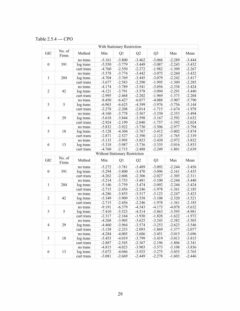
Table 2.5.4 --- CPO With Stationary Restriction
GIC No. ofFirms Method Min Q1 Q2 Q3 Max Mean
0 391no trans -5.161 -3.800 -3.462 -3.066 -2.289 -3.444
log trans -5.550 -3.779 -3.449 -3.087 -2.243 -3.432curt trans -4.760 -2.550 -2.272 -1.982 -1.309 -2.267
1 284no trans -5.578 -3.774 -3.442 -3.075 -2.260 -3.432
log trans -4.704 -3.769 -3.445 -3.079 -2.242 -3.417curt trans -3.677 -2.583 -2.290 -1.995 -1.309 -2.285
2 42no trans -4.174 -3.789 -3.541 -3.056 -2.338 -3.424
log trans -4.121 -3.791 -3.578 -3.094 -2.291 -3.440curt trans -2.995 -2.468 -2.202 -1.969 -1.373 -2.204
3 5no trans -8.450 -6.427 -6.077 -4.088 -3.907 -5.790
log trans -6.963 -6.625 -4.399 -3.976 -3.756 -5.144curt trans -2.278 -2.208 -2.014 -1.715 -1.674 -1.978
4 29no trans -4.160 -3.778 -3.567 -3.330 -2.353 -3.494
log trans -5.618 -3.844 -3.598 -3.167 -2.592 -3.632curt trans -2.924 -2.199 -2.040 -1.757 -1.392 -2.024
5 18no trans -5.832 -3.922 -3.730 -3.506 -2.977 -3.794
log trans -5.128 -4.304 -3.767 -3.412 -3.002 -3.874curt trans -2.871 -2.527 -2.390 -2.125 -1.765 -2.339
6 13no trans -5.133 -3.995 -3.853 -3.430 -2.972 -3.832
log trans -5.318 -3.987 -3.736 -3.335 -3.016 -3.833curt trans -4.760 -2.715 -2.488 -2.249 -1.801 -2.639
Without Stationary Restriction
GIC No. ofFirms Method Min Q1 Q2 Q3 Max Mean
0 391no trans -5.272 -3.781 -3.489 -3.092 -2.244 -3.456
log trans -5.294 -3.800 -3.470 -3.096 -2.161 -3.435curt trans -4.262 -2.606 -2.306 -2.027 -1.305 -2.311
1 284no trans -5.214 -3.753 -3.481 -3.100 -2.244 -3.440
log trans -5.146 -3.759 -3.474 -3.092 -2.244 -3.424curt trans -2.715 -2.456 -2.246 -1.978 -1.361 -2.185
2 42no trans -4.286 -3.855 -3.517 -3.123 -2.247 -3.423
log trans -5.349 -3.909 -3.558 -3.108 -2.320 -3.521curt trans -2.715 -2.456 -2.246 -1.978 -1.361 -2.185
3 5no trans -9.191 -6.379 -4.343 -4.173 -4.078 -5.632
log trans -7.410 -5.523 -4.514 -3.863 -3.595 -4.981curt trans -2.317 -2.164 -1.930 -1.828 -1.622 -1.972
4 29no trans -4.268 -3.905 -3.625 -3.243 -2.382 -3.503
log trans -4.460 -3.964 -3.574 -3.253 -2.623 -3.546curt trans -3.158 -2.253 -2.093 -1.869 -1.377 -2.077
5 18no trans -4.284 -4.005 -3.686 -3.451 -3.015 -3.696
log trans -5.453 -4.019 -3.799 -3.419 -3.013 -3.815curt trans -2.887 -2.545 -2.367 -2.196 -1.806 -2.341
6 13no trans -4.815 -4.023 -3.903 -3.573 -3.108 -3.836
log trans -5.072 -4.046 -3.925 -3.275 -3.055 -3.765curt trans -3.081 -2.669 -2.449 -2.278 -1.603 -2.446
29

Since the distributions of CPO are quite symmetrical without long tails, this chapter uses
the mean value as a major criterion to analyze CPO. The following conclusions are for
the case with stationary restriction.
• Under no transformation, the mean value of CPO ranges from -5.709 (GIC = 3) to
-3.424 (GIC = 2) and -3.444 overall (GIC = 0).
• Under log transformation, the mean value of CPO ranges from -5.144 (GIC = 3)
to -3.417 (GIC = 1) and -3.432 overall (GIC = 0).
• Under cubic root transformation, the mean value of CPO ranges from -2.639 (GIC
= 6) to -1.978 (GIC = 3) and -2.267 overall (GIC = 0).
• For each GIC group, the mean values of CPO are much larger under cubic root
transformation than under log transformation. Also, they have smaller values
under no transformation than under either of the two transformations. These facts
put a lot weight on using both log and cubic root transformations in the Bayesian
analysis of the Ohlson model.
After analyzing the empirical results of the four criteria, this paper goes back to the
decisions that need to make. Since all criteria show the improvement of using log
transformation and cubic root transformation, this paper decides to use two models for
further Bayesian analysis, which are log trans of OFM AR(1) and curt trans of
OFM AR(1).
Since using the transformed scale shows more sensible results, this paper decide to keep
it and stop using the original scale in the following two chapters.
About the restriction stationarity, Nandram & Petruccelli (1997) states that restricting
stationary series to be stationary provides no new information, but restricting
nonstationary series to be stationary leads to substantial differences from the unrestricted
case. In this paper, the results of both average lengths of the credible intervals and CPO
show the benefits of restricting stationarity. Besides, the time plots of the time series for
the companies show that most series look stationary and a few do not. Therefore, this
paper decides to use the stationary restriction in further Bayesian analysis.
30

In summary, the individual Bayesian analysis in this chapter strongly improves the
predictive ability of the Ohlson model comparing to the classical analysis in Chapter 1.
The grouping analysis in Chapter 3 and adaptive analysis by pooling information across
companies in Chapter 4 will be applied to the two transformed models with stationary
restriction. Most further results will be collected under the transformed scale.
31

Chapter 3
Bayesian Data Analysis within Each GIC Group
3.1 Bayesian Version of the Ohlson Model for a GIC Group
As another extreme case, this chapter assumes that all the companies in the same GIC
group share the same parameters ,,, 2
~σρµβ and the GIC groups are independent of each
other, having their own regression coefficients in the Ohlson model. The same structure
as in Chapter 2 is used in this chapter. First of all, a Bayesian version of the Ohlson
model for the grouping analysis is set up in the following three steps.
Step 1, describe the observation ),,,,,,,,,,,,( 1112222111211~
NTNTT yyyyyyyyyy =
by the parameters ,,, 2
~σρµβ , where N is the number of companies in the GIC group,
and T is the number of time periods. Under the assumption that the observations are
independent among the companies, we can get the following likelihood function:
.),|(),|(
),,,|(
1 2
2
~
'
1,~1,~
'
~
2
~
'
1~1
2
~~
∏ ∏= = −
−
−+⋅+=
N
k
T
t tktkktktkk xyxyNxyN
yp
σβρβσµβ
σρµβ
(3.1.1)
Step 2, assign a prior distribution to each parameter.
),,|()(),1,1|()(
),,|()(
),,|()(
22
200
00~~~
baIUN
NK
σσπρρπ
σµµµπ
θββπ
Γ=−=
=
∆=
(3.1.2)
where
(P3.1) yXXXB ')'( 1
0~
−==θ , where ( )'
~
'
1~
'
1~
'
12~
'
11~,,,,,,,
NTNTxxxxxX = .
32
(P3.2) PNT
SSXX E
−=∆ −1
0 )'(100 , where~~~
''' yXByySSE −= , N is the number of
companies, T is the number of observations and P is the number of regression coefficients
(including the intercept).
(P3.3) )()(1 1
~
10 ∑∑
= =
− −=N
j
T
i ijij BxyNTµ .
(P3.4) pNT
SSE
−=2
0σ .
(P3.5) 001.0== ba .
The ideas in choosing those hyperparameters ,,, 2000
0~σµθ ∆ are the same as the ideas in
choosing the hyperparameters in Chapter 2. That is, use the estimation of parameters
from two ordinary linear regression models: (OLM-3) and (OLM-4).
. , ,1;,,1),,0(~ , 2
~
' TtNiNxyiid
itititit ==+= σεεβ (OLM-3)
.,,2,1;,,2,1),,0(~, 2
~
' TtNiNxy itititit ==+−= σεεβµ (OLM-4)
Assume that all the parameters are independent of each other, the joint distribution of the
parameters can be expressed as
).,|(),1,1|(),|(),|(),,,( 22000
0~~
2
~baIUNNp K σρσµµθβσρµβ Γ⋅−⋅⋅∆= (3.1.3)
Step 3, from the likelihood function in (3.1.1) and joint prior distribution in (3.1.3), we
can get the posterior distribution of the parameters given the data by Bayes’ rule:
),|()1,1|(),|(),|(
),|(),|(
)|,,,(
2200
~~
1 2
2
~
'
1,~1,
~
'
~
2
~
'
1~1
~
2
~
baIUNN
xyxyNxyN
yp
P
N
i
T
t titiititii
σρσµµθβ
σβρβσµβ
σρµβ
Γ−∆⋅
−+⋅+∝ ∏ ∏
= = −−
(3.1.4)
33

3.2 Gibbs Sampling
The process of applying Gibbs sampler in this chapter is the same as in Chapter 2.
Without repeating the steps, this section only specifies the complete conditional
distributions for the parameters and the starting points for each parameter.
The complete conditional distributions for the parameters are as follows.
First,
ΛΣΛ+Λ− β
βµθβσρµβ ,)(|~,,,|~~~
2
~~INy P , where
( )
.)()()()(
,
,)(2)(
11111111111
1 2
'
1,~~1,~~
'
1~1~
1 2
'1,1,
'
1~1
1
1 2
'
1,~~1,~~
'
1~1~~
−−−−−−−−−−−
= = −−
= =−−
−
= = −−
∆+Σ∆=∆∆+∆Σ=ΣΣ+∆Σ=ΣΣ+∆=Λ
−
−+=Σ
−−−−⋅
−
−+=
∑ ∑
∑ ∑
∑ ∑
βββββββ
β
β
ρρ
ρρµ
ρρµ
N
i
T
t tiittiitii
N
i
T
ttiittiit
ii
N
i
T
t tkkttiitii
xxxxxx
yyyyxy
xxxxxx
Second,
Φ
−Φ+Φ− ∑
=
2
1 ~
'
1~10
2
~~,)1(~,,,| σβµµσρβµ
N
i ii xyNy , where 22
0
20
σσσ+
=Φ .
Third,
−
−
−
−−
∑∑∑∑
∑∑
= = −−
= = −−
= = −−
N
i
T
t titi
N
i
T
t titi
N
i
T
t titi
itit
xyxy
xyxyNUy
1 2
2
~
'
1,~1,
2
1 2
2
~
'
1,~1,
1 2 ~
'
1,~1,
~
'
~2
~~,)1,1|(~,,,|
β
σ
β
ββρσµβρ
Fourth,
++Γ
2,
2~,,,|
~~
2 SbTNaIy ρµβσ , where
∑∑∑= = −
−=
−−−+
−−=N
i
T
t titi
itit
N
i ii xyxyxyS
1 2
2
~
'
1,~1,
~
'
~1
2
~
'
1~1 βρβµβ .
This chapter chooses the starting points ),,,( 0,2000 σµρβ as follows.
First, ~
10
~')'( yXXX −=β .
34
Second, )2)(1(,1 1,~1,~
1
112
2211
120 ∑∑= +
+
−
=
−−−−==N
i titiit
T
tit aveBxyaveBxySS
SSSSSS
ρ , where
.)1(
)(2 ,
)1(
)(1
,)2(
,)1(
1 ~21 ~
1
1
1
2
~222
1
2
~
1
111
−
−=
−
−=
−−=
−−=
∑∑∑∑
∑∑
∑∑
= ==
−
=
− =
=
−
=
TN
Bxyave
TN
Bxyave
aveBxySS
aveBxySS
N
i t
T
tt
N
i t
T
tt
N
i it
T
tit
N
i it
T
tit
Fourth, ∑∑= =
− −=N
i
T
t itit BxyNT1 1
~
10 )()(µ .
Fifth, pNT
SSE
−=0,2σ .
The ideas of setting 00 , µβ and 0,2σ are the same as the ones of setting the hyper-
parameters ,,, 2000
0~σµθ ∆ in (3.1.2), which is using the estimation of parameters from
the (OLM-3) and (OLM-4). The idea of setting 0ρ is taking it as the autocorrelation of
time series ittiit
itit vxyv ερβ +=−= −1,~
'
~ in an AR(1) structure.
3.3 Forecast
After getting the posterior distribution of the parameters, we can use it to predict the
future stock prices at period T + 1 for each firm in the group ,N, , , i y Ti 211, =+ , given
the data ,N, , ), i ,y,,y(yy iTii(iT) 2121 == . Letting ,,, 2
~σρµβ=Ω , the predictions
can be sampled from the posterior predictive distribution
∫ ΩΩΩ= ++ dyyyfyyf TiiTTi )|()|,()|( 1,)(1, π . (3.3.1)
Letting )()2()1( ,,, MΩΩΩ be a sequence of range M from the Gibbs sampler, an
estimator of )|( )(1, iTTi yyf + is
35
∑=
+−
+ Ω=M
hiT
hTiiTTi yyfMyyf
1)(
)(1,
1)(1, ),|()|(ˆ . (3.3.2)
To get samples of 1, +Tiy , we use data argumentation to fill in 1, +Tiy to each )(hΩ ,
Mh , ,2 ,1 = to get )(1,
hTiy + , Mh , ,2 ,1 = from the normal distribution described below.
)),((~,| 2
~
'
~~
'
1,~)(1, σβρβiT
iTTi
iTTi xyxNyy −+Ω+
+ (3.3.3)
The 95% predictive credible interval for 1, +Tiy can be computed from the 2.5% and
97.5% empirical quantiles of the values )(1,
hTiy + , Mh , ,2 ,1 = .
3.4 Conditional Predictive Ordinate
In this chapter, the conditional predictive ordinate is defined as
,,2,1 ,,,2,1
,),|()|(1
)()(
1,)(
)(1,
TtNi
yypyypM
hit
hti
hititti
==
Ω≈ ∑=
++ ϖ (3.4.1)
where 1, +tiy denotes the random future observation of company i at period t + 1,
),,,( 21)( itiiit yyyy = denotes the observations of company i from period 1 to t,
)(hΩ denotes the hth draw of the parameters from the Gibbs sampler,
and
.,,1,
)|()|(
)|()|(
1)(
)()(
)(
)()(
)( Mh
yfyfyf
yf
M
kh
hit
h
hit
hit =
ΩΩ
ΩΩ
=
∑=
ϖ
3.5 Empirical Results of Grouping Bayesian Analysis
The same criteria as in Chapter 2 are used for the model valuation in this chapter. Table
3.5.1 shows the quantiles of R under the transformed scale as well as numbers of positive
ratios and negative ratios averaged in each GIC group with stationary restriction, from
36

which we can draw the following conclusions. In order to be consistent with Chapter 2,
Q2 is used as a major criterion in analyzing R .
• Based on Q2, the ratio value ranges from -0.7% (GIC = 1) to 2.3% (GIC = 5) and
0.4% over all (GIC = 0) under log transformation and from -0.7% (GIC = 1) to
3% (GIC = 5) and 0.8% over all (GIC = 0) under cubic root transformation.
• Based on Q2, for the same GIC group, the ratio under log transformation is no
bigger than under cubic root transformation. This implies that log transformation
is better for group analysis.
• Under both transformations, the numbers of positive ratios and negative ratios for
each group are very close and 0.5 is between LB and UB, which indicates that
both transformations do not overestimate the stock prices. The only exception is
in the case with GIC equal to 0 under cubic root transformation.
Table 3.5.1 --- Quantiles of Ratio & Numbers of Nonnegative/Negative RatiosWith Stationary Restriction
GIC No. of Firms Method Min Q1 Q2 Q3 Max No.
(+,0)No.(-) LB UB
0 391 log trans -2.728 -0.074 0.004 0.083 2.220 200 191 0.486 0.537curt trans -1.082 -0.073 0.008 0.092 1.386 206 185 0.502 0.552
1 284 log trans -2.678 -0.072 0.000 0.076 2.090 142 142 0.470 0.530curt trans -0.899 -0.073 0.004 0.085 1.179 146 138 0.484 0.544
2 42 log trans -0.520 -0.073 -0.007 0.061 0.689 20 22 0.399 0.553curt trans -0.499 -0.078 -0.007 0.067 0.605 20 22 0.399 0.553
3 5 log trans -2.217 -0.198 0.008 0.218 2.064 3 2 0.381 0.819curt trans -2.078 -0.193 0.014 0.223 1.820 3 2 0.381 0.819
4 29 log trans -0.831 -0.096 0.011 0.120 1.508 15 14 0.424 0.610curt trans -0.882 -0.103 0.013 0.131 1.381 15 14 0.424 0.610
5 18 log trans -0.804 -0.075 0.023 0.124 1.112 10 8 0.438 0.673curt trans -0.911 -0.076 0.030 0.141 1.174 10 8 0.438 0.673
6 13 log trans -1.617 -0.158 0.022 0.206 2.270 7 6 0.400 0.677curt trans -1.678 -0.166 0.026 0.221 2.089 7 6 0.400 0.677
Table 3.5.2 gives minimum, maximum and overall values of R under the transformed
scale from both classical statistical analysis and grouping Bayesian analysis. It shows the
magnificent improvement of using grouping Bayesian approach to the Ohlson model
compared to the classical method.
37

Table 3.5.2 --- Min, Max and Overall Values of RMethod Transformation min max overall
Classical log trans 4.70% 9.80% 8.80%Analysis curt trans 6.30% 13.80% 10.90%Grouping log trans -0.70% 2.30% 0.40%Analysis curt trans -0.70% 3% 0.80%
Table 3.5.3 --- Average Length of Credible Interval
GIC
No. ofFirms Method
With S-RestrictionAve
LengthStd Dev
0 391log trans 1.241 0.235curt trans 1.215 0.228
1 284log trans 1.168 0.226curt trans 1.164 0.222
2 42log trans 1.071 0.007curt trans 1.059 0.007
3 5log trans 4.040 0.207curt trans 3.753 0.195
4 29log trans 1.988 0.288curt trans 1.994 0.292
5 18log trans 1.880 0.189curt trans 1.941 0.198
6 13log trans 3.446 0.260curt trans 3.413 0.264
Table 3.5.3 gives the average length of credible intervals and the corresponding standard
deviations for both log transformation and cubic root transformation under the
transformed scale and with the stationary restriction, from which we can draw the
following conclusions.
• Under log transformation, the average length of CI ranges from 1.071 (GIC = 2) to
4.040 (GIC = 3) and 1.241 overall (GIC = 0), the standard deviation ranges from
0.007 (GIC = 2) to 0.288 (GIC = 4) and 0.235 overall (GIC = 0).
• Under cubic root transformation, the average length of CI ranges from 1.059 (GIC
= 2) to 3.753 (GIC = 3) and 1.215 overall (GIC = 0), the standard deviation ranges
from 0.007 (GIC = 2) to 0.292 (GIC = 4) and 0.228 overall (GIC = 0).
38
• For each GIC group, the average length of CI is slightly smaller under cubic root
transformation than under log transformation.
Table 3.5.4 --- Conditional Predictive Ordinate (each group has its own parameters)With Stationary Restriction
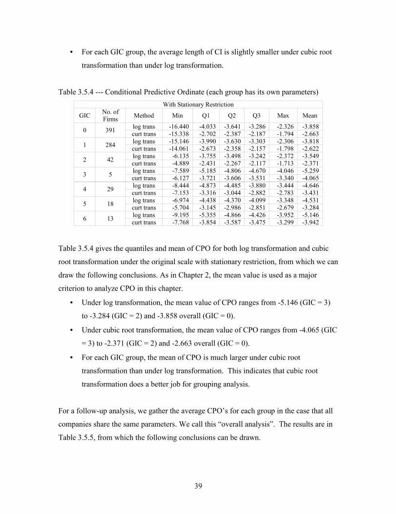
GIC No. ofFirms Method Min Q1 Q2 Q3 Max Mean
0 391 log trans -16.440 -4.033 -3.641 -3.286 -2.326 -3.858curt trans -15.338 -2.702 -2.387 -2.187 -1.794 -2.663
1 284 log trans -15.146 -3.990 -3.630 -3.303 -2.306 -3.818curt trans -14.061 -2.673 -2.358 -2.157 -1.798 -2.622
2 42 log trans -6.135 -3.755 -3.498 -3.242 -2.372 -3.549curt trans -4.889 -2.431 -2.267 -2.117 -1.713 -2.371
3 5 log trans -7.589 -5.185 -4.806 -4.670 -4.046 -5.259curt trans -6.127 -3.721 -3.606 -3.531 -3.340 -4.065
4 29 log trans -8.444 -4.873 -4.485 -3.880 -3.444 -4.646curt trans -7.153 -3.316 -3.044 -2.882 -2.783 -3.431
5 18 log trans -6.974 -4.438 -4.370 -4.099 -3.348 -4.531curt trans -5.704 -3.145 -2.986 -2.851 -2.679 -3.284
6 13 log trans -9.195 -5.355 -4.866 -4.426 -3.952 -5.146curt trans -7.768 -3.854 -3.587 -3.475 -3.299 -3.942
Table 3.5.4 gives the quantiles and mean of CPO for both log transformation and cubic
root transformation under the original scale with stationary restriction, from which we can
draw the following conclusions. As in Chapter 2, the mean value is used as a major
criterion to analyze CPO in this chapter.
• Under log transformation, the mean value of CPO ranges from -5.146 (GIC = 3)
to -3.284 (GIC = 2) and -3.858 overall (GIC = 0).
• Under cubic root transformation, the mean value of CPO ranges from -4.065 (GIC
= 3) to -2.371 (GIC = 2) and -2.663 overall (GIC = 0).
• For each GIC group, the mean of CPO is much larger under cubic root
transformation than under log transformation. This indicates that cubic root
transformation does a better job for grouping analysis.
For a follow-up analysis, we gather the average CPO’s for each group in the case that all
companies share the same parameters. We call this “overall analysis”. The results are in
Table 3.5.5, from which the following conclusions can be drawn.
39
• Under log transformation, the mean value of CPO ranges from -4.429 (GIC = 2)
to -3.401 (GIC = 4).
• Under cubic root transformation, the mean value of CPO ranges from -3.183 (GIC
= 2) to -2.176 (GIC = 4).
• For each GIC group, the mean of CPO is much larger under cubic root
transformation than under log transformation. This indicates that cubic root
transformation does a better job than log transformation for the overall analysis.
Table 3.5.5 --- Conditional Predictive Ordinate (all companies have the same parameters)With Stationary Restriction
GIC No. ofFirms Method Min Q1 Q2 Q3 Max Mean
1 284 log trans -16.442 -4.002 -3.625 -3.279 -2.326 -3.827curt trans -15.338 -2.692 -2.383 -2.191 -1.794 -2.659
2 42 log trans -9.295 -4.990 -3.998 -3.560 -2.428 -4.429curt trans -7.924 -3.598 -2.630 -2.338 -1.852 -3.183
3 5 log trans -4.657 -4.456 -3.812 -3.065 -2.579 -3.714curt trans -3.323 -3.108 -2.568 -2.121 -1.875 -2.599
4 29 log trans -4.033 -3.783 -3.360 -3.061 -2.495 -3.401curt trans -2.473 -2.327 -2.152 -2.013 -1.915 -2.176
5 18 log trans -4.437 -4.161 -3.739 -3.568 -3.139 -3.814curt trans -2.943 -2.568 -2.412 -2.265 -2.053 -2.434
6 13 log trans -4.738 -4.180 -3.855 -3.453 -2.950 -3.822curt trans -3.236 -2.716 -2.498 -2.249 -2.013 -2.508
Table 3.5.6 provides the comparison of the mean of CPO from Table 3.5.4 and Table
3.5.5. This is the comparison between grouping analysis and overall analysis, from which
we can conclude that: under both transformations, grouping analysis and overall analysis
have almost the same predictive ability within GIC 1, which has the largest number of
companies. Group analysis does a better job than overall analysis in GIC 2 and a worse
job for the left GIC groups.
40

Table 3.5.6 --- Comparison of Table 3.5.3 to 3.5.4
log trans of OFM AR(1)-2GIC Mean-3.5.3 Mean-3.5.4 dif dif/Mean-3.5.3
1 -3.818 -3.827 -0.009 0.0022 -3.549 -4.429 -0.88 0.2483 -5.259 -3.714 1.545 0.2944 -4.646 -3.401 1.245 0.2685 -4.531 -3.814 0.717 0.1586 -5.146 -3.822 1.324 0.257
curt trans of OFM AR(1)-2GIC Mean-3.5.3 Mean-3.5.4 dif dif/Mean-3.5.3
1 -2.622 -2.659 -0.037 0.0142 -2.371 -3.183 -0.812 0.3423 -4.065 -2.599 1.466 0.3614 -3.431 -2.176 1.255 0.3665 -3.284 -2.434 0.85 0.2596 -3.942 -2.508 1.434 0.364
Summarily, the grouping Bayesian analysis in this chapter also greatly improves the
predictive ability of the Ohlson model comparing to the classical analysis in Chapter 1.
It does not overestimate the stock prices under both transformations with stationary
restriction, and cubic root transformation is better than log transformation in this case.
The cubic root transformation is especially applicable for those GIC groups which have
large amount of companies.
41

Chapter 4
Bayesian Data Analysis by Adaptive Pooling
Information Across Firms
4.1 Bayesian Hierarchical Model
The Bayesian approaches in Chapter 2 and Chapter 3 represents two extreme cases.
Chapter 2 treats each company individually and does not borrow information across
companies at all. Chapter 2 overestimates the stock prices. Chapter 3 supposes all the
companies in the same GIC group follow the same rules of predicting stock prices, which
brings more information in the investigation. The improvement in Chapter 3 is correcting
the bias, but the model is too simple. Furthermore, these two extreme cases are barely
seen in the real stock literature where on one side the companies have their own specific
characteristics and on the other side they are affected by the same economic factors and
therefore have some things in common. As a combination of Chapter 2 and Chapter 3,
also in order to be closer to the reality, this chapter develops a hierarchical Bayesian
approach is to simultaneously estimate the unknown coefficients for each company by
adaptively pooling information across firms.
Considering that all the firms will be included in the Ohlson model, it is required to add
the company index into expression (1.1.5) which turns out to be
. , ,1 , , ,1 ), ,0(~
. , ,2 , , ,1,)(
. , ,1 ,
2
~
'
1,~1,~
'
~
1~
'
1~1
TtniN
Ttnixyxy
niuxy
i
iid
it
ititi
tiiiit
it
iiii
i
==
==+−+=
=++=
−−
σε
εβρβ
εβ
(4.1.1)
The Bayesian version of the Ohlson Model in (4.1.1) for a GIC group is set up in four
steps.
42

First, describe the observation ),,,,,,,,,,,,( 1112222111211~
NTNTT yyyyyyyyyy =
by the parameters ,,2,1:,,, 2
~Niiii
i=σρµβ , where N is the number of companies,
and T is the number of time periods. Under the assumption that the observations are
independent among the companies, we can get the following likelihood function:
.),|(),|(
),2,1:,,,|(
1 2
2
~
'
1,~1,~
'
~
2
~
'
1~1
2
~~
∏ ∏= = −
−
−+⋅+=
=
N
i
T
ti
ititiiiititii
iii
iiii
xyxyNxyN
Niyp
σβρβσµβ
σρµβ
(4.1.2)
Second, assuming independence at all levels, assign a prior distribution to each
parameter,
),,|()(
),,|()(
200
~~~
iiii
iK
i
N
N
φψµµπ
θββπ
=
∆=
,,,2,1),/,|()(
),,|()(22
200
NiIN
ii
iiii
=Γ=
=γαασσπ
τνρρπ
(4.1.3)
where ,,,~
γαθ ∆ are unknown hyperparameters, and ,,2,1:,,, 200
200 Niiiii =τνφψ are
known hyperparameters which are set as follows.
(P4.1) )(1
125.0),(10
1
20
10 iii
T
jijiii
T
jiji BXy
TBXy
Tψφψ −−
−⋅=−= ∑∑
==.
(P4.2) 21
1 1,
1
1 1,
)(2
1100,1
1i
T
j iiji
iiiji
T
j iiji
iiiji BXy
BXyTBXy
BXyT
ντν ∑∑−
= +
−
= +
−−
−−
⋅=−
−−
= ,where
),,,(),,,,(,')'( 21211
iTiiiiTiiiiiiii yyyyxxxXyXXXB === − , .,,2,1 Ni =
This paper does not pool si 'ρ because the time series of some companies are stationary
while some are not. It does not pool si 'µ because the start values can be very different
from the rest and it is difficult to pool them. In order to use the information across
43

companies, we pool si 'β adaptively. As for si '2σ , we incorporate heterogeneity but we
believe they come from the same population and allow pooling them.
Third, assign a hyper-prior distribution to each unknown hyperparameter in ,,,~
γαθ ∆ .
(P4.3) ),|(~ 00~~~
∆θθθ PN , ),)(|( 01
0011 νν −−− ∆∆=∆ PWishart ,where
,2,)'(100,')'( 01
0~
1
0~+=
−=∆= −− P
pNTSS
XXyXXX E νθ
( )'
~
'
1~
'
1~
'
12~
'
11~,,,,,,,
NTNTxxxxxX = .
(P4.4) .1)(,)1(
1)(2 γ
γα
α ∝+
∝ pp
Assume that all the parameters ,,2,1:,,, 2
~Niiii
i=σρµβ are independent of each
other, the joint distribution of the parameters can be expressed as
].)/,|(),|(),|(),|([
),2,1:,,,|,2,1:,,,(
1
2200
200
~~
~
2
~
∏=
Γ⋅⋅⋅∆=
=∆=
N
iiiiiiii
iP
iiii
INNN
NiNip
γααστνρφψµθβ
γαθσρµβ
(4.1.4)
Since we have assumed that all the unknown hyperparameters ,,,~
γαθ ∆ are independent
of each other, the joint distribution for the unknown hyperparameters can be expressed as
.)1(
),)(|(),|(),,,( 2
01
001
00~~1
~ αγ
ννθθγαθ
+
∆∆∆∝∆
−−
−WishartN
pP (4.1.5)
Finally, from the likelihood function in (4.1.2) and joint prior distribution in (4.1.4) as
well as in (4.1.5), we can get the posterior distribution of all the parameters by Bayes’
rule:
),,2,1:,,,,,,,|(),,2,1:,,,,,,,(
)|,,2,1:,,,,,,,(
1
~
2
~~
1
~
2
~
~
1
~
2
~
NiypNip
yNip
iiii
iiii
iiii
=∆=∆∝
=∆
−−
−
γαθσρµβγαθσρµβ
γαθσρµβ
44

),,2,1:,,,|(),,2,1:,,,,,,,( 2
~
1
~
2
~NiypNip iii
iiii
i ==∆∝ − σρµβγαθσρµβ
),,2,1:,,,|(),,,(
),,,|,,2,1:,,,(
2
~
1
~
1
~
2
~
Niypp
Nip
iiii
iiii
=∆
⋅∆=∝
−
−
σρµβγαθ
γαθσρµβ
.),|(),|(
)1(
),)(|(),|(
])/,|(),|(),|(),|([
1 2
2
~
'
1,~1,~
'
~
2
~
'
1~1
2
01
001
00~~
1
2200
200~~
∏ ∏
∏
= = −−
−−
=
−+⋅+
⋅+
∆∆∆
⋅Γ⋅⋅⋅∆∝
N
i
T
ti
ititii
iititii
iii
PP
N
iiiiiiii
iP
xyxyNxyN
WishartN
INNN
σβρβσµβ
αγ
ννθθ
γααστνρφψµθβ
(4.1.6)
4.2 Gibbs Sampling
The target here is to make inferences on the parameters ,,2,1:,,, 2
~Niiii
i=σρµβ and
the unknown hyperparameters ,,,~
γαθ ∆ given the data. The complete conditional
distributions are as follows.
First,
ΛΣΛ+Λ−∆−
ii
INyi
Piiii
ββ
µθβγαθσρµβ ,)(|~,,,,,,,|~~~
1
~
2
~~, where
( )
,
,)(2)(
2
'
1,~~1,~~
'
1~1~
2
'1,1,
'
1~1
1
2
'
1,~~1,~~
'
1~1~~
∑
∑
∑
= −−
=−−
−
= −−
−
−+=Σ
−−−−⋅
−
−+=
T
t tii
ittii
itii
T
ttiiittiiit
iii
T
t tki
kttii
itii
xxxxxx
yyyyxy
xxxxxx
i
i
ρρ
ρρµ
ρρµ
β
β
,)()()()( 11111111111 −−−−−−−−−−− ∆+Σ∆=∆∆+∆Σ=ΣΣ+∆Σ=ΣΣ+∆=Λ βββββββ
.,,2,1 Ni =
45

Second,
Φ
−Φ+Φ−∆ ∑
=
− 2
1 ~
'
1~10
1
~
2
~~,)1(~,,,,,,,| ii
N
i iiiiiiii
ii xyNy σβψµγαθσρβµ ,
where 220
20
ii
ii σφ
φ+
=Φ , .,,2,1 Ni =
Third,
++
+∆−
ii
ii
ii
iiiiiii
ii B
BB
ABNy 2
0
20
20
2001
~
2
~~,~,,,,,,,|ττ
ττν
ργαθσµβρ , where
∑∑
∑
= −−
= −−
= −−
−
=
−
−
−
=T
t ititi
iiT
t ititi
T
t ititi
iitit
i
xyB
xy
xyxyA
2
2
~
'
1,~1,
2
2
2
~
'
1,~1,
2 ~
'
1,~1,~
'
~ ,
β
σ
β
ββ, .,,2,1 Ni =
Fourth,
++Γ∆−
2,
2~,,,,,,,| 1
~~~
2 iii
ii
STIyγααγαθρµβσ , where
∑= −
−
−−−+
−−=
T
t ititii
iititi
iiii xyxyxyS
2
2
~
'
1,~1,~
'
~
2
~
'
1~1 βρβµβ , .,,2,1 Ni =
Fifth, where),,(~,,2,1:,,,,,,,| 12
~~~Σ=∆− mNNiy Piii
iγασρµβθ
.,)(0~
10
1 ~
11110
∆+∆Σ=∆+∆=Σ −
=
−−−− ∑ θβN
i imN
Sixth, where),,(~,,2,1:,,,,,,,|~
2
~~
1 HhWishartNiy Piiii
=∆− γαθσρµβ
.))((,1
'
~~~~000 ∑
=
−−+∆=+=N
i iiHNh θβθβνν
Seventh, ).10(1
then ,1
let <<−
=+
= ττ
ταα
ατ
.exp)(~
,,2,1:,,,,,,,,|
11
21
1
2
1
~
2
~~
ττα
αα
σγασ
γαα
αγθσρµβτ
−=
=
−+
=
−−
−
−
Γ
=∆
∏∏N
ii
N
ii
NN
iiii
Niy
Eighth, .,~,,2,1:,,,,,,,|1
21
~
2
~~
Γ=∆ ∑
=
−−N
iiiii
iNINiy σαααθσρµβγ
46

The Gibbs sampling is to carry out the following steps (i) and (ii) iteratively. These two
steps consist of sub-steps that are carried out sequentially for a single chain. The Markov
chain can also be replicated by drawing independent initial values of the parameters and
hyperparameters.
Step (i): Update the parameters ,,2,1:,,, 2
~Niiii
i=σρµβ given the hyperparameters
and data. The following sub-steps (i-1) to (i-4) are executed independently for each
Ni ,,2,1 = .
(i-1) Draw i~
β directly from the multivariate normal distribution described in (4a);
(i-2) Draw iµ directly from the univariate normal distribution described in (4b);
(i-3) Use Devroye (1986) method to draw iρ from the univariate normal distribution
described in (4c);
(i-4) Draw 2iσ directly from the inverse gamma distribution described in (4d).
Step (ii): Generate the hyperparameters ,,,~
γαθ ∆ given the values of the parameters in
step (i).
(ii-1) Draw ~θ from the multivariate normal distribution described in (4e);
(ii-2) Draw ∆ from the P-dimensional Wishart distribution described in (4f);
(ii-3) Use a grid to draw α from the complete conditional distribution described in (4g);
(ii-4) Drawγ from the inverse Gamma distribution described in (4h).
4.3 Forecasting
After getting the posterior distribution of the parameters, we can use it to predict the
future stock prices at period T + 1 for each firm in the group ,N, , , i y Ti 211, =+ , given
the data ,N, , ), i ,y,,y(yy iTii(iT) 2121 == .
47

Letting ,,,, 2
~iii
ii σρµβ=Ω ,,,2,1 Ni = the predictions can be sampled from the
posterior predictive distribution
.)|()|,()|( 1,)(1, ∫ ΩΩΩ= ++ iiiTiiTTi dyyyfyyf π (4.3.1)
Letting )()2()1( ,,, Miii ΩΩΩ be a sequence of range M from the Gibbs sampler, an
estimator of )|( )(1, iTTi yyf + is
∑=
+−
+ Ω=M
hiT
hiTiiTTi yyfMyyf
1)(
)(1,
1)(1, ),|()|(ˆ . (4.3.2)
To get samples of 1, +Tiy , we use data argumentation to fill in 1, +Tiy to each )(hiΩ ,
Mh , ,2 ,1 = to get )(1,
hTiy + , Mh , ,2 ,1 = from the normal distribution described below:
).),((~,| 2
~
'
~~
'
1,~)(1, iiiT
iTiiTi
iTiTi xyxNyy σβρβ −+Ω+
+ (4.3.3)
The 95% predictive credible interval for 1, +Tiy can be computed from the 2.5% and
97.5% empirical quantiles of the values )(1,
hTiy + , Mh , ,2 ,1 = .
4.4 Conditional Predictive Ordinate
In this chapter, the conditional predictive ordinate is defined as
,,2,1 ,,,2,1
,),|()|(1
)()(
1,)(
)(1,
TtNi
yypyypM
hit
hiti
hititti
==
Ω≈ ∑=
++ ϖ (4.4.1)
where 1, +tiy denotes the random future observation of company i at period t + 1,
),,,( 21)( itiiit yyyy = denotes the observations of company i from period 1 to t, )(hiΩ
denotes the hth draw of the parameters from the Gibbs Sampler, and
.,,1,
)|()|(
)|()|(
1)(
)()(
)(
)()(
)( Mh
yfyfyf
yf
M
kh
i
hiit
hi
hiit
hit =
ΩΩ
ΩΩ
=
∑=
ϖ
48

4.5 Empirical Results of Adaptive Bayesian Analysis by Pooling Information Across
Firms
As in Chapter 2 or 3, the same criteria are used for the model valuation in this chapter.
Table 4.5.1 --- Quantiles of Ratio & Numbers of Nonnegative/Negative RatiosWith Stationary Restriction
GIC No. of Firms Method Min Q1 Q2 Q3 Max
No.(+,0)
No.(-) LB UB
0 391 log trans -8.3252 -0.1449 0.0609 0.2805 9.1655 226 165 0.553 0.603curt trans -3.2252 -0.1460 0.0641 0.2868 3.5102 227 164 0.556 0.606
1 284 log trans -8.3252 -0.1489 0.0581 0.2791 9.1655 163 121 0.545 0.603curt trans -3.2252 -0.1514 0.0600 0.2838 3.5102 163 121 0.545 0.603
2 42 log trans -5.2459 -0.1490 0.0812 0.3287 4.2113 25 17 0.519 0.671curt trans -3.0397 -0.1431 0.0880 0.3372 3.1222 25 17 0.519 0.671
3 5 log trans -1.2484 -0.1413 0.0649 0.2749 2.8667 3 2 0.381 0.819curt trans -1.2718 -0.1385 0.0741 0.2915 2.9801 3 2 0.381 0.819
4 29 log trans -1.6030 -0.1239 0.0606 0.2475 1.6233 17 12 0.495 0.678curt trans -1.6576 -0.1227 0.0669 0.2612 1.6809 17 12 0.495 0.678
5 18 log trans -2.1939 -0.1253 0.0631 0.2636 2.1197 11 9 0.439 0.661curt trans -2.2456 -0.1240 0.0707 0.2793 2.0704 11 9 0.439 0.661
6 13 log trans -1.8886 -0.1332 0.0617 0.2735 2.4346 8 5 0.480 0.750curt trans -1.9548 -0.1358 0.0630 0.2786 2.2311 8 5 0.480 0.750
Table 4.5.1 shows the quantiles of ratio under the transformed scale as well as numbers of
positive ratios and negative ratios averaged in each GIC group with stationary restriction,
from which we can draw the following conclusions.
• Based on Q2, the ratio value ranges from 5.81% (GIC = 1) to 8.12% (GIC = 2)
and 6.09% overall (GIC = 0) under log transformation, and from 6% (GIC = 1) to
8.8% (GIC = 2) and 6.41% overall (GIC = 0)under cubic root transformation.
Under both transformations, GIC 1 has the smallest ratio and GIC 5 has the largest
ratio.
• Based on Q2, for the same GIC group, the ratio under log transformation is
smaller than under cubic root transformation.
• When GIC is 0, 1 or 2, 0.5 is not between LB and UB; when GIC is 3, 4, 5, or 6,
0.5 is between LB and UB. This indicates that both transformations overestimate
the stock price for large GIC groups and do not overestimate the stock price for
small GIC groups.
49

Table 4.5.2 --- Min, Max and Overall Values of RMethod Transformation min max overall
Classical log trans 4.70% 9.80% 8.80%Analysis curt trans 6.30% 13.80% 10.90%
Adaptive Pooling log trans 5.81% 8.12% 6.09%Analysis curt trans 6% 8.80% 6.41%
Table 4.5.3 --- Average Length of Credible Interval
GIC No. of Firms Method
With S-RestrictionAve. CI Length
Std Dev
0 391log trans 4.085 0.453curt trans 3.873 0.450
1 284log trans 4.064 0.458curt trans 3.854 0.455
2 42log trans 4.292 0.452curt trans 4.056 0.444
3 5log trans 4.232 0.484curt trans 3.990 0.573
4 29log trans 3.868 0.369curt trans 3.668 0.367
5 18log trans 4.233 0.331curt trans 4.052 0.358
6 13log trans 4.040 0.357curt trans 3.856 0.367
Table 4.5.2 gives minimum, maximum and overall values of R under the transformed
scale from both classical statistical analysis and adaptive pooling Bayesian analysis. It
shows the notable improvement of using adaptive pooling Bayesian approach to the
Ohlson model compared to the classical method.
Table 4.5.3 gives the average length of credible intervals and the corresponding standard
deviations for both log transformation and cubic root transformation under the
transformed scale with stationary restriction, from which we can draw the following
conclusions.
50
• Under log transformation, the average length of CI ranges from 3.868 (GIC = 4) to
4.292 (GIC = 2) and 4.085 overall (GIC = 0), the standard deviation ranges from
0.331 (GIC = 5) to 0.573 (GIC = 3) and 0.453 overall (GIC = 0).
• Under cubic root transformation, the average length of CI ranges from 3.668 (GIC
= 4) to 4.056 (GIC = 2) and 3.873 overall (GIC = 0), the standard deviation ranges
from 0.358 (GIC = 5) to 0.573 (GIC = 3).
• For each GIC group, the average length of CI is significantly smaller under cubic
root transformation than under log transformation.
Table 4.5.4 --- Conditional Predictive Ordinate With Stationary Restriction
GIC No. ofFirms Method Min Q1 Q2 Q3 Max Mean
0 391 log trans -2.558 -1.387 -1.274 -1.203 -1.054 -1.306cube root trans -2.381 -1.337 -1.225 -1.142 -0.995 -1.250
1 284 log trans -2.558 -1.358 -1.268 -1.202 -1.063 -1.296cube root trans -2.381 -1.310 -1.216 -1.135 0.995 -1.240
2 42 log trans -1.750 -1.497 -1.397 -1.242 -1.084 -1.384cube root trans -1.687 -1.430 -1.341 -1.173 -1.016 -1.322
3 5 log trans -1.638 -1.586 -1.478 -1.250 -1.162 -1.423cube root trans -1.586 -1.526 -1.423 -1.164 -1.100 -1.360
4 29 log trans -1.661 -1.275 -1.216 -1.144 -1.054 -1.228cube root trans -1.610 -1.230 -1.164 -1.086 -0.995 -1.173
5 18 log trans -1.675 -1.483 -1.378 -1.270 -1.160 -1.389cube root trans -1.628 -1.426 -1.327 -1.212 -1.093 -1.338
6 13 log trans -1.479 -1.353 -1.207 -1.212 -1.134 -1.282cube root trans -1.440 -1.324 -1.197 -1.155 -1.059 -1.235
Table 4.5.4 gives the quantiles and mean of CPO for both log transformation and cubic
root transformation under the transformed scale with stationary restriction, from which
we can draw the following conclusions.
• Under log transformation, the mean value of CPO ranges from -1.423 (GIC = 3)
to -1.228 (GIC = 4) and -1.306 overall (GIC = 0).
• Under cubic root transformation, the mean value of CPO ranges from -1.360 (GIC
= 3) to -1.173 (GIC = 4) and -1.250 overall (GIC = 0).
• Under both transformations, group 4 has the largest CPO and group 3 has the
smallest CPO.
51

• For each GIC group, the mean of CPO is quite larger under cubic root
transformation than under log transformation. This indicates that cubic root
transformation does a better job than log transformation for the approach of
adaptive pooling information across companies.
In all, the adatpive Bayesian analysis by pooling information across companies in this
chapter still improves the predictive ability of the Ohlson model comparing to the
classical analysis in Chapter 1. It overestimates the stock price under both
transformations with stationary restriction when the size of GIC group is large, and
doesn’t overestimate the stock price when the size is small. Cubic root transformation is
better than log transformation in this case.
52
Chapter 5
Comparison of Three Bayesian Models and
Overall Conclusions
In this last chapter, we present the conclusions of our research work on forecasting stock
prices via the Ohlson model after comparing the three Bayesian models.
5.1 Comparison of Three Bayesian Models
This section first compares the three Bayesian models that are used the former three
chapters based on the minimum, maximum and overall values of R, average length of
credible interval and log conditional predictive ordinate (CPO), which are gathered in
Table 5.1.1. All these values are on the transformed scale except that CPO’s are
calculated on the original scale.
The following conclusions can be drawn from Table 5.1.1.
• Based on R, grouping analysis has the smallest R values (less than 1%) and
adaptive pooling analysis has the largest R values (around 6.5%). The individual
analysis results in very small R values too (around 2%).
• Based on average length of credible interval, individual analysis has the shortest
lengths (around 1) and adaptive pooling analysis has the longest lengths (around
4). The average length values got from grouping analysis are not large (around
1.2).
• Based on CPO, individual analysis has the largest values (greater than -1.5), and
adaptive pooling analysis has comparable values with grouping analysis (mostly
less than -2).
53
Theoretically, adaptive pooling analysis is supposed to achieve the best predictive results.
But using the criteria above, adaptive pooling analysis does not show any advantages
comparing to the other two methods.
Table 5.1.1
Method R Transformation min max overall
Individual log trans 0.50% 2.50% 2%Analysis curt trans 0.70% 2.90% 2.20%Grouping log trans -0.70% 2.30% 0.40%Analysis curt trans -0.70% 3% 0.80%
Adaptive Pooling log trans 5.81% 8.12% 6.09%Analysis curt trans 6% 8.80% 6.41%
Method Ave Length of CI Transformation min max overall
Individual log trans 0.652 1.003 0.949Analysis curt trans 0.682 1.012 0.958Grouping log trans 1.071 4.04 1.241Analysis curt trans 1.059 3.753 1.215
Adaptive Pooling log trans 3.868 4.292 4.085Analysis curt trans 3.668 4.056 3.873
Method CPOTransformation min max overall
Individual log trans -5.144 -3.417 -3.432Analysis curt trans -2.639 -1.978 -2.267Grouping log trans -5.146 -3.284 -3.858Analysis curt trans -4.065 -2.371 -2.663
Adaptive Pooling log trans -6.046 -3.245 -4.737Analysis curt trans -4.233 -2.810 -3.429
For the adaptive Bayesian analysis, two transformations are also compared based on the
same criteria as above. This paper concludes that log transformation and cubic
transformation are comparable even though the results show that the cubic root
transformation does a slightly better job.
In the former three chapters, LB and UB that are calculated by the number of nonnegative
R’s and the number of negative R’s are used to check the state of overestimation. The
conclusion is both individual analysis and adaptive pooling analysis overestimate the
stock prices, but the grouping analysis does not. To have an overall look, see Table 5.1.2.
54
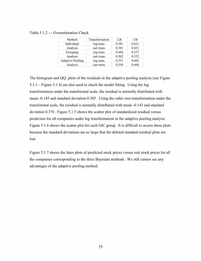
Table 5.1.2 --- Overestimation Check
Method Transformation LB UBIndividual log trans 0.581 0.631Analysis curt trans 0.581 0.631Grouping log trans 0.486 0.537Analysis curt trans 0.502 0.552
Adaptive Pooling log trans 0.553 0.603Analysis curt trans 0.556 0.606
The histogram and QQ- plots of the residuals in the adaptive pooling analysis (see Figure
5.1.1 – Figure 5.1.4) are also used to check the model fitting. Using the log
transformation under the transformed scale, the residual is normally distributed with
mean -0.145 and standard deviation 0.385. Using the cubic root transformation under the
transformed scale, the residual is normally distributed with mean -0.143 and standard
deviation 0.370. Figure 5.1.5 shows the scatter plot of standardized residual versus
prediction for all companies under log transformation in the adaptive pooling analysis
Figure 5.1.6 shows the scatter plot for each GIC group. It is difficult to access these plots
because the standard deviations are so large that the deleted standard residual plots are
lost.
Figure 5.1.7 shows the lines plots of predicted stock prices versus real stock prices for all
the companies corresponding to the three Bayesian methods. We still cannot see any
advantages of the adaptive pooling method.
55

Figure 5.1.1
Qunf ang 30APR05
-2. 175 -1. 875 -1. 575 -1. 275 -0. 975 -0. 675 -0. 375 -0. 075 0. 225 0. 525 0. 825 1. 125 1. 425
0
2. 5
5. 0
7. 5
10. 0
12. 5
15. 0
17. 5
Percent
resi dual
Figure 5.1.2
56

Figure 5.1.3
Qunf ang 30APR05
-2.175 -1. 875 -1. 575 -1. 275 -0. 975 -0. 675 -0. 375 -0. 075 0.225 0.525 0. 825 1. 125 1. 425
0
2. 5
5. 0
7. 5
10. 0
12. 5
15. 0
17. 5
Percent
resi dual
Figure 5.1.4
Qunf ang 30APR05
-4 -2 0 2 4
-3
-2
-1
0
1
2
residual
Normal Quanti l es
57

Figure 5.1.5
Figure 5.1.6
58

Figure 5.1.7
59

5.2 Estimated Regression Coefficients from Adaptive Bayesian Analysis
In Chapter 1, the classical approach gives the estimated regression coefficients for each
GIC group and concludes that the intercept, BPS and the first two following quarters’
abnormal earnings per share ( 41 ~ ββ ) are generally significant in the Ohlson Model.
To compare with this conclusion, the posterior distribution of ~θ in the Bayesian model
for adaptive pooling analysis for each GIC group are collected in Table 5.2.1, which
shows that only the intercept, BPS and the first following quarters’ abnormal earnings per
share ( 31 ~ ββ ) are significant. A reduced model with only these three predictors is
analyzed by the adaptive pooling Bayesian approach. Those three items turn out to be all
significant in the reduced model (see Table 5.2.2).
Table 5.2.1 --- Summaries of the Posterior Distribution of ~θ for the Full Model
log trans with stationary restrictionParameters Mean STD NSE C025 C975
theta1 3.20899 0.07187 0.01513 3.0697 3.35517theta2 0.02597 0.00682 0.00117 0.01221 0.03906theta3 0.1982 0.09071 0.01886 0.02582 0.38316theta4 0.1283 0.07958 0.01441 -0.01576 0.28409theta5 0.02232 0.07982 0.0163 -0.14066 0.18115theta6 -0.00458 0.07225 0.0149 -0.14558 0.14257
curt trans with stationary restrictionParameters Mean STD NSE C025 C975
theta1 2.89697 0.06865 0.01438 2.76542 3.0369theta2 0.02877 0.00641 0.00111 0.01611 0.04133theta3 0.21271 0.08863 0.01808 0.03906 0.39566theta4 0.13214 0.07454 0.01371 -0.00397 0.28132theta5 0.01312 0.07821 0.01577 -0.14944 0.16467theta6 -0.0048 0.0693 0.01426 -0.14041 0.14078
Note that STD denotes the posterior standard deviation, NSE denotes the numerical
standard error, C025 and C975 denote the lower bound and upper bound of the 95%
credible interval separately.
60

Table 5.2.2 --- Summaries of the Posterior Distribution of ~θ for the Full Model
log trans with stationary restrictionParameters Mean STD NSE C025 C975
theta1 3.20442 0.06307 0.02058 3.07917 3.32686theta2 0.02736 0.00539 0.00149 0.01648 0.03735theta3 0.23281 0.05942 0.01453 0.11947 0.35121
curt trans with stationary restrictionParameters Mean STD NSE C025 C975
theta1 2.88904 0.061 0.02002 2.76801 3.00891theta2 0.03011 0.00513 0.00143 0.01991 0.03958theta3 0.24232 0.05713 0.01409 0.13454 0.3568
5.3 Overall Conclusions
Overall, four approaches are applied to interpret the Ohlson model in this paper. They are
classical statistical analysis in Chapter 1, individual Bayesian analysis in Chapter 2,
grouping Bayesian analysis in Chapter 3 and adaptive pooling Bayesian analysis in
Chapter 4. The first two chapters prove that both the log transformation and cubic root
transformation can enhance the predictive ability of the Ohlson model. The analysis in
Chapter 2 results to use stationary restriction and transformed measurement scale. All
three Bayesian approaches are compared to the classical method based on the minimum,
maximum and overall values of R, and they are also compared with each other based on
the same criteria. The conclusions are:
• Each Bayesian approach used in this paper does better job than the classical
method
• Log transformation and cubic transformation have comparable efficiency in
enhancing the predictive ability.
• Book value per share and the abnormal earning per share for the first following
period affect the stock prices significantly, the last three abnormal earnings are not
important.
This paper expects to reach the conclusion that the adaptive pooling Bayesian method is
better than individual or grouping Bayesian approach. But all the four criteria, relative
difference (R), average length of credible interval, lower bound (LB) and upper bound
61

(UB) of the 95% credible interval of the estimated probability of nonnegative R, and log
conditional predictive ordinate (CPO), all fail to give this sensible conclusion. Further
investigations are necessary.
62

Appendices
63

A. Origination of the Ohlson (1995) Valuation Model
For more accurate understanding, this paper splits the commonly called Ohlson (1995)
model into two: the Ohlson (1995) Valution Model (OVM) and the Ohlson (1995)
Approximation Model (OAM). The Ohlson (1995) Valution Model is a special case of
the Residual Income Valuation Model (RIM), which was developed from the traditional
Dividend Discount Model (DDM).
In economics and finance, the traditional approach to the problem of stock valuation
based on a single firm has focused on the Dividend Discount Model (DDM) of
Rubinstein (1976). It defines the value of a firm as the present value of the expected
future dividends. That is, under the assumption of no arbitrage, there exists a pricing
kernel itit r −
+ += )1(π such that the price of a stock tP is related to its dividends td by
,)1(11
+=
= ∑∑
∞
=+
−∞
=++
iit
itt
iitittt drEdEP π (A1)
where tr denotes the discount rate during time period t, [.]tE denotes the expectations
operator conditioned on the date t information. Note that the “arbitrage” is a situation in
which the company can make money by exploiting the efficiency of the market.
The idea of DDM implies that one should forecast dividends in order to estimate the
stock prices. Since dividends are arbitrarily decided by management, it may be hard to
estimate a dividend process in small samples (Ang & Liu, 1998). Moreover, market
participants tend to focus on accounting information, especially earnings. The
fundamental relation between book value of equity tbv , earnings tx and dividends td is
described in the Clean Surplus Accounting Model by equation tttt dxbvbv −+= −1 , i.e.,
the change in book value between two dates equals earnings minus dividends. This
relations is called the Clean Surplus Relation (CSR) which can also be written as
).( 1−−−= tttt bvbvxd (A2)
64

Substituting equation (A2) to equation (A1), thereby eliminating dividends, yields the
Residual Income Valuation Model (RIM) described in Peasnell (1982). It is a function of
only accounting variables, namely:
.)()1(1
1∑∞
=−++
− −++=i
ittiti
ttt bvrxrbvP (A3)
This principle shows that the theoretical value of the firm is equal to the opening book
value of equity plus the present value of its residual income (or excess earning), and will
not be affected by accounting choices.
The attention to the relationship between theoretical firm value and the residual income
stream has attracted considerable practitioner interest and resulted in a number of
proprietary models being marketed (Gregory, Saleh & Tucker, 2004). The Ohlson (1995)
Valuation Model (OVM), one special case of the general class of RIM, is evaluated as a
“major breakthrough” (Bernard, 1995) and “landmark works in financial accounting”
(Lundholm, 1995). The particular innovation in the Ohlson model is the employment of
an “AR(1) linear information dynamic” (LID) which is comprised of abnormal earnings
and a variable tv representing “other information” whose source is uncorrelated with
accounting information. We can view the abnormal earnings as a contraction of “above
normal earnings”. The terminology is motivated by the concept that “normal” earnings
should relate to the “normal” return on the capital invested at the beginning at the period,
that is, net book value at date t – 1 multiplied by the interest rate tr . Thus one interprets
atx as earnings ( tx ) minus a charge for the use of capital ( 1, −titbvr ) as in the following
equation:
1−−= tttat bvrxx . (A4)
The LID assumption can be written formally as
+=++=
++
++
1,21
1,1111
ttt
tatt
at
vvxvx
εγεϖ
--- AR(1) Linear Dynamic (A5)
65

where 11ϖ is persistence parameter of abnormal earnings atx , 1,21,1 , ++ tt εε is white noise
error terms with zero mean, γ is persistence parameter of other information tv .
Substituting equations (A4) and (A5) to RIM, yields the Ohlson Valuation Model:
,11 tattt vxbvP βα ++=
(A6)
where
.)1(
1,
1 111
111 ϖ
βϖ
α−+
+=
−=
tt
t
t rrr
r
(See Appendix B for the derivation process.)
The Ohlson model states that the stock price is a linear function of book value of the
equity ( tbv ), current abnormal earnings and an intercept term, which takes the following
regression form:
tattt xbvP εβββ +++= 210 (A7)
66

B. Derivation of the Ohlson Valuation Model
The following is the straightforward derivation process of equation (A7):
][)1(
)0][(][)1(][)1()1(
][)1(
][)1(
11
11
11
111
1
1111
1
aitt
i
it
t
tt
ittiti
ti
ta
itti
it
i
ittt
ita
ittti
itt
aitt
i
ittt
xErrv
bv
EErxErrvbv
xvErbv
xErbvP
−+
∞
=
−
++
∞
=
−−+
∞
=
−∞
=
−
+−+
∞
=
−
+
∞
=
−
∑
∑∑∑
∑
∑
+++=
=++++++=
++++=
++=
ϖ
εεϖ
εϖ
][)1(1 )1(
1
)1(11 aitt
i
it
tt
tt xEr
rrv
bv −+
∞
=
−−∑ ++
++=ϖ
)(11
][)1(1
][1
][)1(1
1111
1
1111
0
11
ttt
at
tt
tt
aitt
i
it
t
att
tt
tt
aitt
i
it
tt
tt
bvPr
xrr
vbv
xErr
xErr
vbv
xErrr
vbv
−+
++
++=
++
++
++=
++
++=
+
∞
=
−
+
∞
=
−
∑
∑
ϖϖ
ϖϖ
ϖ
at
ttt
tttt
at
tt
t
tt
tttt
at
ft
t
t
ttt
xrrr
vrbvP
xrr
rrr
vrbvP
xRr
vr
rbvP
11
11
1
11
11
11
1111
1)1()1(
)1)(1()1(
)1()1(
11)(
ϖϖ
ϖ
ϖϖ
ϖ
ϖϖ
−++
−+++=⇒
+−++
+−+
+=−⇒
+=
+−+−⇒
67

C. The Ohlson Approximation (1995) Model
Ohlson (1995) presents us with the license to break with the traditional focus on
explaining price behavior and to shift that focus to predicting earnings. The key lies in
the following approximation. It states that the value of the firm can be well approximated
even over a finite horizon by a function of forecasted earnings, book value, and discount
rates. The only assumption required is that these forecasts be consistent with clean
surplus relation. We begin by defining a variable TtV as follows:
].[)1(1)1(
)1(1
1−++
=
− −+−+
++= ∑ τττ
τtttt
T
tTt
Tt
tT
t bvrxErr
rbvV (C1)
Note that the amount TtV is a function of future earnings and book values measured over
a finite horizon. However, despite the limited horizon, T
tV approximates the value of the
firm, so long as the horizon is “long enough”, which can be described as the following
equation:
.lim tT
tTPV =
∞→ (C2)
Equations (C1) and (C2) imply that the ability to predict earnings and book value --- even
over a finite horizon --- is tantamount to the ability to approximate current value. For a
special empirical application of the Ohlson (1995) approximating model, we use the
future earnings and book value forecasted over a horizon of 4 periods. That is, we let T =
4. Equation (C1) turns out to be
].[)1(1)1(
)1(1
4
14
44
−++=
− −+−+
++= ∑ τττ
τttttt
t
ttt bvrxEr
rrbvV (C3)
If 4tV provides a good approximation of firm value, we should be able to explain a large
fraction of the variation in stock prices with the variables on the right-hand side of
equation (C3). This suggests the following regression model:
.][ 1,,
4
11,10 ittittitiitiiit vbvrxEbvP +−++= −++
=+∑ ττ
ττβββ (C4)
Model (C4) is the Ohlson Model used in this paper.
68

D. Definitions of Data Items
(All the definitions are for industrials.)
DOW JONES INDUSTRY GROUP represents the industry classification assigned by
Dow Jones based on the company’s lines of business.
GENERAL INSTUSTY CLASSIFICATION represents a company's general industry
classification. 01 Industrial; 02 Utility; 03 Transportation; 04 Banks/Savings and Loan;
05 Insurance; 06 Other Financial
DOW JOE MARKET SECTORS are a standardized series of digits that are used to
categorize market segments issued by Dow Jones.
The Global Industry Classification Standard (GICS) was developed by Morgan Stanley
Capital International (MSCI), a premier independent provider of global indices and
benchmark-related products and services, and Standard & Poor’s (S&P), an independent
international financial data and investment services company and a leading provider of
global equity indices.
The GICS classifications aim to enhance the investment research and asset management
process for financial professionals worldwide. It is the result of numerous discussions
with asset owners, portfolio managers and investment analysts around the world and is
designed to respond to the global financial community’s need for an accurate, complete
and standard industry definition.
GICSSECTOR means GICS Codes. The following websites are about the sector
definitions.
http://www.msci.com/equity/GICS_Sector_Definitions_2005.pdf
COMPANY IDENTITY KEY (ID)
69

PRICE CLOSE means the last price an issue traded at for that day. For the quarterly data
set of PriceClose, all the values are the last price for the last day of corresponding quarter.
TOTAL ASSETS represent the sum of total current assets, long term receivables,
investment in unconsolidated subsidiaries, other investments, net property plant and
equipment and other assets.
TOTAL LIABILITIES represent all short and long term obligations expected to be
satisfied by the company.
It includes:
(1) Current Liabilities
(2) Long Term Debt
(3) Provision for Risk and Charges (non-U.S. corporations)
(4) Deferred taxes
(5) Deferred income
(6) Other liabilities
(7) Deferred tax liability in untaxed reserves (non-U.S. corporations)
(8) Unrealized gain/loss on marketable securities (insurance companies)
(9) Pension/Post retirement benefits
(10) Securities purchased under resale agreements (banks)
It excludes:
(1) Minority Interest
(2) Preferred stock equity
(3) Common stock equity
(4) Non-Equity reserves
PREFERRED STOCK represents a claim prior to the common shareholders on the
earnings of a company and on the assets in the event of liquidation.
For U.S. corporations, its value is shown at the total involuntary liquidation value of the
number of preferred shares outstanding at year end. If preferred stock is redeemable at
70

anytime by the shareholder it is shown at redemption value, or if the company carries it at
a higher value than the involuntary liquidation value, the stated value.
Preferred stock of subsidiary and premium on preferred stock is included in preferred
stock. It excludes minority interest in preferred stock.
For Non-U.S. Corporations, the stated value of preferred stock is shown and it includes
all preferred stock related accounts.
For Non-U.S. Corporations preference stock which participates with the
common/ordinary shares in the profits of the company is included in common equity.
COMMON SHARES OUTSTANDING represent the number of shares outstanding at the
company's year end. It is the difference between issued shares and treasury shares.
For companies with more than one type of common/ordinary share, common shares
outstanding represents the combined shares adjusted to reflect the par value of the share
type identified in field 6005 - Type of Share.
BOOK VALUE PER SHARE represents the book value (proportioned common equity
divided by outstanding shares) at the company's fiscal year end for non-U.S. corporations
and at the end of the last calendar quarter for U.S. corporations.
Preference stock has been included in equity and the calculation of book value per share
where it participates with common/ordinary shares in the profits of the company. It is
excluded in all other cases, deducted at liquidation value for U.S. companies and at par
value for all others.
EARNINGS PER SHARE means the portion of a company's profit allocated to each
outstanding share of common stock.
EPSMeanQTR1 is the mean value in a set of EPS estimates of the first fiscal quarter for a
company; EPSMeanQTR2 is the mean value in a set of EPS estimates of the second fiscal
quarter for a company. Same ideas can be adopted by EPSMeanQTR2 and
EPSMeanQTR3. (See Table 2 for more details.)
71

EPSConsensusForecastPeriodQTR1 is the period (month) for which an EPS estimate is
being forecasted. Same ideas can be adopted to EPSConsensusForecastPeriodQTR3-4.
(See Table 3 for more details.)
Table 2 EPSMeanQTR1 (partly)
Key: Feb-98 Mar-98 Apr-98 May-98 Jun-98 Jul-98C000003104 0.5 0.5 0.5 0.53 0.46 0.46C000000048 0.39 0.38 0.37 0.37 0.37 0.34C000028595 0.54 0.54 0.54 0.56 0.56 0.56C000000006 0.06 0.06 0.06 0.06 0.07 0.07C000000085 0.12 0.12 0.11 0.11 0.1 0.14C000001268 0.24 0.23 0.23 0.24 1.03 1.02C000000104 -0.07 -0.09 -0.08 -0.08 -0.09 -0.08C000000020 0.17 0.17 0.17 0.2 0.2 0.19C000000110 0.93 0.92 0.84 0.94 0.94 0.92C000029653 0.17 0.17 0.17 0.17 0.17 0.18C000000015 0.19 0.19 0.19 0.19 0.19 0.18
Table 3 EPSConsensusForecastPeriodQTR1 (partly)
Key: Feb-98 Mar-98 Apr-98 May-98 Jun-98 Jul-98C000003104 Mar1998 Mar1998 Mar1998 Jun1998 Jun1998 Jun1998C000000048 Mar1998 Mar1998 Jun1998 Jun1998 Jun1998 Sep1998C000028595 Mar1998 Mar1998 Mar1998 Jun1998 Jun1998 Jun1998C000000006 Apr1998 Apr1998 Apr1998 Apr1998 Jul1998 Jul1998C000000085 Feb1998 Feb1998 May1998 May1998 May1998 Aug1998C000001268 Mar1998 Mar1998 Mar1998 Mar1998 Jun1998 Jun1998C000000104 Mar1998 Mar1998 Jun1998 Jun1998 Jun1998 Sep1998C000000020 Mar1998 Mar1998 Mar1998 Jun1998 Jun1998 Jun1998C000000110 Mar1998 Mar1998 Mar1998 Jun1998 Jun1998 Jun1998C000029653 Mar1998 Mar1998 Mar1998 Mar1998 Mar1998 Jun1998C000000015 Mar1998 Mar1998 Mar1998 Jun1998 Jun1998 Jun1998
Treasury bills are short-term debt instruments used by the U.S. Government to finance
their debt. Commonly called T-bills they come in denominations of 3 months, 6 months
and 1 year. Each treasury bill has a corresponding interest rate (i.e. 3-month T-bill rate, 1-
year T-bill rate).
72

E. How to retrieve data by Thomsom ONE Analytics Excel Add-in
For instance, we want to retrieve the data set of PriceClose.
1. Make sure you have Microsoft Excel installed in your computer.
2. Download and install the software “Thomson ONE Analytics Excel Add-in”.
1) Open the Thomson ONE Banker Analytics Web page.
2) Click on “Tools” at the top of the Thomson One page.
3) Click on the “Office Tools” tab on the Tools page.
4) See the section “Thomson ONE Analytics for Office Version 1.0”.
5) Click on the “Download” link in this section and follow the directions to save the
add-in installation file to your computer.
6) There are brief installation directions on this page, and step-by-step installation
instructions also can be downloaded from this section. During the installation
process, your Thomson Analytics username and password must be entered. Once
installed, the Thomson Analytics Toolbar will be visible in Excel.
3. Upload S&P500 into Thomson Analytics, call 800-662-7878(-1-2) for help.
4. In a blank Excel sheet, choose the first cell (A1).
5. On the Thomson Analytics toolbar,
1) Click on Wizards.
2) Choose Report Wizards.
3) In “Step 2”, click “Add Entities”.
4) On the pop-up window, click “Download”.
5) Choose SP500 and click “OK”.
6) On the returned window, click “OK” again.
7) In “Step 1”, click “Add/Edit items”.
8) Under “Data Items For”, click on the pull-down button, choose “Datastream”.
9) Under “Search for Item”, input “priceclose”, double click “priceclose” in the
window below. Then click “OK”.
10) In “Step 3”, under “Starting Period”, click on the button with an icon of calendar.
First choose “Quarterly”, then choose “Q1” of “1998”; under “Ending Period”,
use the same way to choose “Q1” of “2004”.
73

11) Click “Next”.
12) Click “Finish”.
13) On the pop-up window, choose “No”. You can get the PriceClose data set of
SP500 in a spreadsheet.
14) Save the file.
74

F. How to extract quarterly data out of monthly data
Companies forecast their expected earnings every month for the following four fiscal
quarters. Note that the fiscal quarters may have different starting and ending months
from the calendar quarters. Different companies may have different definitions of their
fiscal quarters.
This paper uses the latest forecast value for each quarter to represent the corresponding
quarter value. Based on this idea, there are 4 steps to get quarterly data out of monthly
data. For instance, we want to get the quarterly data of EPSMeanQTR1 in Table 2.
Table 4 Transformed EPSConsensusForecastPeriodQTR1 (partly)
ID Feb-98 Mar-98 Apr-98 May-98 Jun-98 Jul-983104 2 2 2 3 3 348 2 2 3 3 3 428595 2 2 2 3 3 36 2 2 2 2 3 385 1 1 2 2 2 31268 2 2 2 2 3 3104 2 2 3 3 3 420 2 2 2 3 3 3110 2 2 2 3 3 329653 2 2 2 2 2 315 2 2 2 3 3 3
1. Replacing the values in each row in Table 3 (EPSConsensusForecastPeriodQTR1)
with 1 to 4 by increasing 1 each time from the earliest date to the latest date, which
results in Table 4.
2. Find out the last forecast month for each fiscal quarter and represent it with 1. All
other forecast months are set to be 0. This can be done by the command “diff” in
MatLab. The result can be shown in Matrix 1.
3. Construct a matrix (Matrix 2) containing the values of EPSMeanQTR1 in Table 3.
4. Find out the expected earning corresponding to each quarter. This can be done by dot
multiplying (“.*”) Matrix 1 to Matrix2, which results in Matrix 3.
75

5. Extract the quarterly expected earning by deleting all the 0 from Matrix 3. This can
be done by command “B=A(A>0)”, where A refers to the revised form Matrix 3, B is
the quarterly data matrix. Note that this command only works when each row of A
has the same amount of positive values. In application, A needs to be adjusted to
satisfy this requirement. Also note that some expected earnings are negative and some
are zeros. In order not to miss this values, we can add a relative large positive value,
say 10, to each item in order to make them positive. After getting the quarterly data
matrix, 10 can be subtracted to get the real values.
Matrix 1
0 0 1 0 0 10 1 0 0 1 00 0 1 0 0 10 0 0 1 0 00 1 0 0 1 00 0 0 1 0 00 1 0 0 1 00 0 1 0 0 00 0 1 0 0 10 0 0 0 1 10 0 1 0 0 1
Matrix 2
0.5 0.5 0.5 0.53 0.46 0.460.39 0.38 0.37 0.37 0.37 0.340.54 0.54 0.54 0.56 0.56 0.560.06 0.06 0.06 0.06 0.07 0.070.12 0.12 0.11 0.11 0.1 0.140.24 0.23 0.23 0.24 1.03 1.02
-0.07 -0.09 -0.08 -0.08 -0.09 -0.080.17 0.17 0.17 0.2 0.2 0.190.93 0.92 0.84 0.94 0.94 0.920.17 0.17 0.17 0.17 0.17 0.180.19 0.19 0.19 0.19 0.19 0.18
76

Matrix 3
0 0 0.5 0 0 0.460 0.38 0 0 0.37 00 0 0.54 0 0 0.560 0 0 0.06 0 00 0.12 0 0 0.1 00 0 0 0.24 0 00 -0.09 0 0 -0.09 00 0 0.17 0 0 00 0 0.84 0 0 0.920 0 0 0 0.17 0.180 0 0.19 0 0 0.18
77

G. Derivation of CPO
∫∫ ΩΩΩ=ΩΩ= +++ dyyypdyypyyp ttttttt )|(),|()|,()|( )()(1)(1)(1 π
Mkyf
yfyf
yf
yfyf
yfyf
yfyf
yfyf
yyy
y
yfyf
yfyf
yfyfyfyf
yfypyfyp
yy
yyy
y
yyp
yy
M
yy
yypM
dyy
y
dyy
yyyp
dyy
yyyp
M
kk
kt
k
kt
M
k tk
kt
tk
kt
M
kk
tk
kt
k
kt
t
tttttt
M
kk
tk
kt
k
kt
M
k
ktt
kt
M
kk
tk
M
kk
tk
ktt
t
ttt
ttt
,,1)|()|(
)|()|(
)()(
)|()|(
)()(
)|()|(
)|()|(
)|()|(
)()(
)|()|(
)(/)()|()(/)()|(
)(/),()(/),(
)|()|(
)|()|(
)|()|(
),|(
)|()|(
)|()|(
),|(
)|()|()|(
)|()|()|(
),|(
)|()|()|(
),|(
1)(
)()(
)(
)()(
1 )()(
)()(
)()(
)()(
1)(
)()(
)()(
)(
)(
)(
)()()()()()(
1)(
)()(
)()(
)(
)(
1
)()(1)(
1)(
)()(
1
1)(
)()(
)()(1
1
)(
)()(1
)()(1
=ΩΩ
ΩΩ
=⋅
ΩΩ
⋅ΩΩ
=
ΩΩΩ
Ω
=
⋅ΩΩ
=ΩΩΩΩ
=ΩΩ
=Ω
ΩΩ
ΩΩ
Ω
=
Ω=
ΩΩ
ΩΩ
Ω≈
ΩΩΩ
Ω
ΩΩΩ
ΩΩ
=
ΩΩΩ
ΩΩ=
∑∑∑
∑
∑
∑
∑
∫
∫
∫
===
=
=+
=
−
=+
−
+
+
πππ
π
ϖ
ππ
ππ
πππ
π
ϖ
ϖ
ππ
ππ
ππ
π
ππ
π
ππ
π
78

References
Ohlson J. 1995. Earning, book value and dividends in security valuation.
Contemporary Accounting Research 11: 661-687.
Bernard V. 1995. The Feltham-Ohlson framework: implications for empiricists.
Contemporary Accounting Research 11: 733-747.
Feltham G,.& Ohlson J. 1995. Valuation and clean surplus accounting for operating and
financial activities. Contemporary Accounting Research 11: 684-731.
Callen. J,. & Morel M. 2001. Linear accounting valuation when abnormal earnings are
AR(2). Review of Quantitative Finance and Accounting 16: 191-203.
Ota K. 2002. A test of the Ohlson (1995) model: empirical evidence from Japan.
The International Journal of Accounting 37: 157-182.
Nandram B, Petruccelli J. 1997. A Bayesian analysis of autoregressive time series panel
data. Journal of Business & Economic Statistics 15: 328-334.
Ying & Kuo 2003. Forecasting stock prices using a hierarchical Bayesian approach.
Unpublished Research Paper.
Albert J, Chib S. 1993. Bayesian analysis via Gibbs sampling of autoregressive time
series subject to Markov mean and variance shifts. Journal of Business and
Economic Statistics 11: 1-15.
Gelfand AE, Hills S, Racine-Poon A, Smith AFM. 1990. Illustration of Bayesian
inference in normal data models using Gibbs sampling. Journal of American
Statistical Association 85: 972-985.
79

Rosenberg M, Andrews, R, Lenk P. 1999. A hierarchical Bayesian model for predicting
the rate of non-acceptable in-patient hospital utilization. Journal of Business and
Economic Statistics 17: 1-8.
Wakefield J, Smith AFM, Racine-Poon A, Gelfand AE. 1994. Bayesian analysis of linear
and non-linear population models by using the Gibbs sampler. Applied Statistician
43: 201-221.
80
Recommended