Mark P. Baldwin, University of Exeter
Imperial College
12 December 2012
Stratosphere–Troposphere Coupling
in a Changing Climate
Mark P. Baldwin

(From Baldwin and Dunkerton, Science 2001)
Long Timescale

Text
60 days following weak stratospheric winds 60 days following strong stratospheric winds
Observed Average Surface Pressure Anomalies (hPa)
From Baldwin et al., Science 2001

Northern Annular Mode
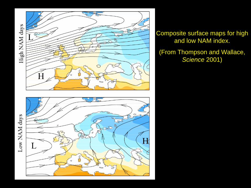
Composite surface maps for high
and low NAM index.
(From Thompson and Wallace,
Science 2001)
>0.9°C

7
• No one has yet explained the dynamics of how
the troposphere is affected.
• I think that any “theory” of stratosphere–
troposphere coupling must account for the main
observations:
1) the surface pressure pattern associated with
variations in the strength of the polar vortex looks
like the NAM/NAO.
2) the maximum surface response is near the North
Pole.
3) the relationship between stratospheric vortex
strength and the NAM is linear.

8
• Baldwin and Dunkerton (1999) suggested that
the redistribution of mass in the stratosphere, in
response to changes in wave driving, may be
sufficient to influence the surface pressure
significantly, consistent with the theoretical
results of Haynes and Shepherd (1989).
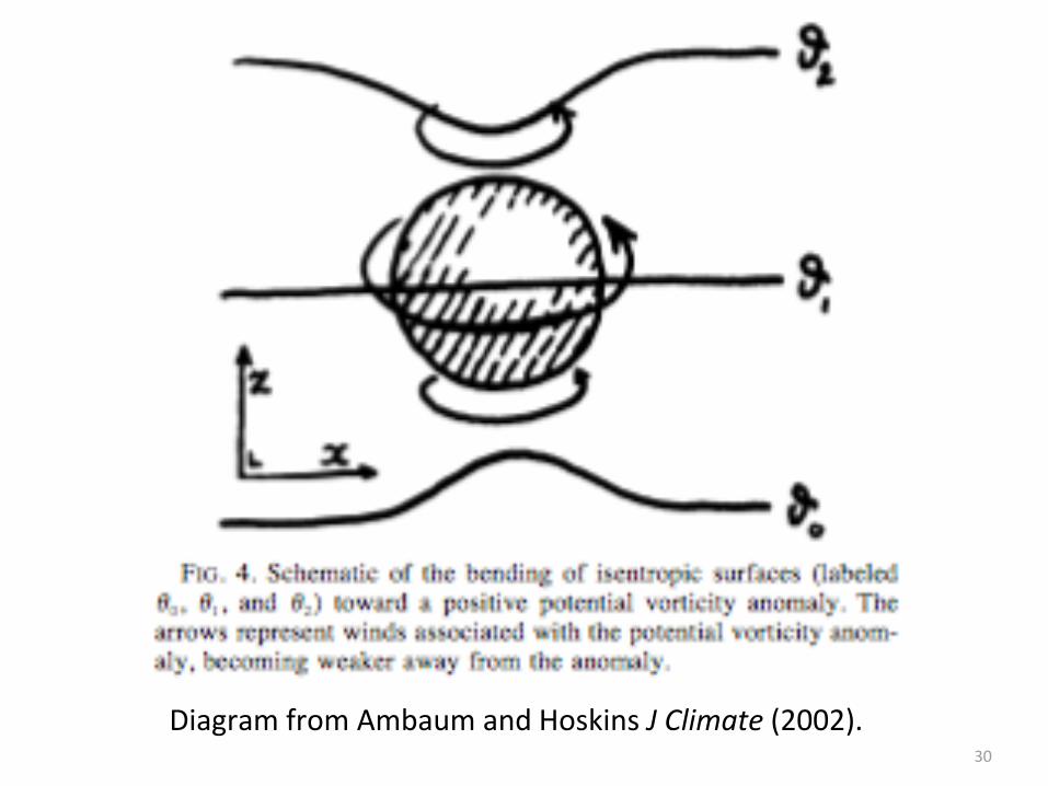
• Ambaum and Hoskins (2002) used “PV
thinking” to explain how stratospheric PV
anomalies affect surface pressure.

Wave Drag
Anomalous wave drag leads to variations in vortex strength
“Wave Driven Pump”

25
Diagram from Ambaum and Hoskins J Climate (2002).

26
Polar cap “PV600K Index” ~20-25 hPa
Create an index of vortex strength as defined by PV at 600K (20-25 hPa).

28 From Baldwin and Birner, Nature Geosci., under revison

29
Weak Vortex
Event
Strong Vortex
Event
From Baldwin and Birner, Nature Geosci., under revision
30
Diagram from Ambaum and Hoskins J Climate (2002).

31

35
Correlation during winter (JFM) between the 600K PV index and zonal-mean temperature. The JFM daily correlation between PV530 and polar cap tropopause T anomalies is 0.90.
From Baldwin and Birner, Nature Geosci., under revision

38

39
Higher pressure and temperature
Mass
Polar cap
A simple “model”
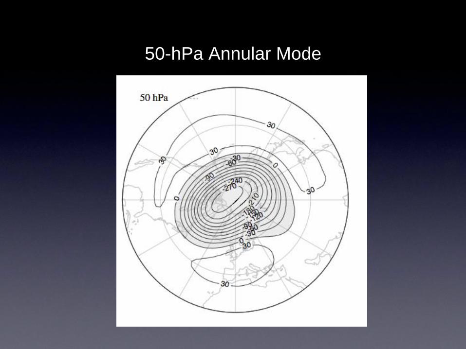
50-hPa Annular Mode
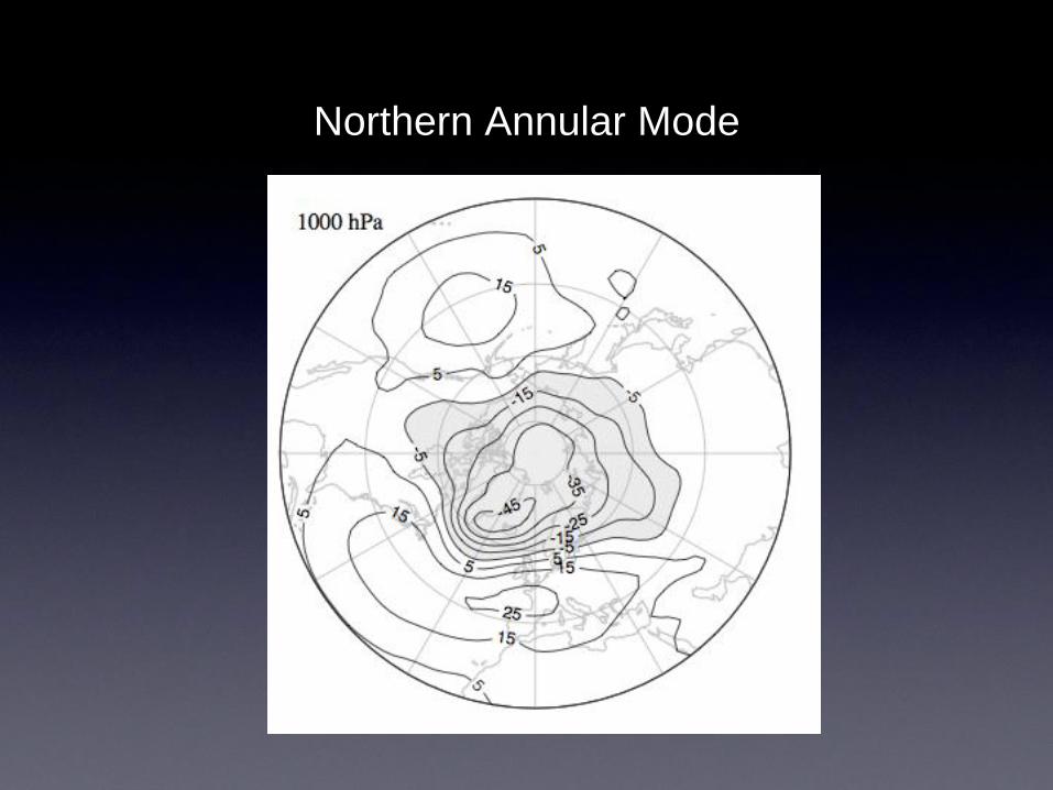
Northern Annular Mode

42
Changing the depth of the troposphere affects 1) vorticity in the column, and 2) surface pressure.
Plunger

43
Changing the depth of the troposphere affects 1) vorticity in the column, and 2) surface pressure.
Wave driven pump
Rigid boundary at 65N

44
Changing the depth of the troposphere affects 1) vorticity in the column, and 2) surface pressure.
modest tropospheric effect?
A guess at tropospheric pressure change
wave driven pump

45
ERA-40 observations
Regression between PV600K index and Polar Cap p’
Tropospheric amplification
Actual Data
This diagnostic can be made for any model or data set.

46
Conclusions
• The physics is the same for monthly or climate-change time
scales.
• Both PV theory and mass movement explains 1) why the
surface pattern looks like the NAM, and why the surface
effects are proportional to anomalies in the strength of the
polar vortex.
• S–T coupling is easily diagnosed in models, including
changes on long time scales. The simple ∆P vs. Z
diagnostic can be used to assess the realism of S–T
coupling in any model.
Recommended