Balanced Pricing in
Microfinance:
Setting Prices to Balance the Needs of the
Institution and the Clients
Chuck Waterfield, CEO
MicroFinance Transparency
15 July 2015

B a l a n c e d P r i c i n g i n M i c r o f i n a n c e P a g e | 2
OUR GOAL FOR THIS PROPOSAL
After decades of ignorance and neglect about the true prices that we were charging the poor, we have made
great progress in the past seven years. We now have definitions and measurements for a large portion of
the global industry.
However, we still struggle on interpretation of our prices. Sadly, the current standards promoted for judging
pricing all have weaknesses and can easily lead to erroneous conclusions. Partly, this is because we are still
learning about pricing. Pricing of microcredit is an exceedingly difficult concept to understand, and despite
three decades of studying pricing, I am the first to say I am still learning. Yet despite the challenges, we
should try even harder; pricing is as important a subject as it is a difficult subject.
I propose here an approach to evaluate the degree to which an MFI is achieving balanced pricing. Balance
means the MFI is not heavily centered on its own self-interest, nor is it operating heavily on the expectation
that donors will fund operations. The MFI looks for solutions that achieve balance between the two sides of
the business transaction — itself and the
poor — rather than leave that ethical
responsibility to the pressures that are
assumed to eventually come from the
market's invisible hand. A responsible
business proactively and intentionally makes
balanced policy decisions rather than
waiting for the market to force it to do so.
I present the rationale of this approach and
then show how that logic is incorporated in
the software "MFT Pricing Analysis Tool"
which can be downloaded from
www.mftransparency.org. In this paper, I also highlight areas where the approach can be improved with
additional refinements to the logic. I invite your feedback and ideas via email at
[email protected]. In the last part of this paper I give some initial ideas of how the implications of
the balanced pricing concept apply to three different types of MFIs:
those providing only larger microloans, e.g., ProCredit
Those with broad market coverage, e.g., BancoSol
Those who provide only the smallest of microloans, with loan sizes under 25% of GNI per capita,
e.g., Compartamos
Microfinance has considered these all as the same market, but these three markets are as different from
one another as microfinance is different from conventional finance.

B a l a n c e d P r i c i n g i n M i c r o f i n a n c e P a g e | 3
LOGIC OF BALANCED PRICING
Beware of Averages!
A central principal in this Balanced Pricing methodology is the same principle that has been at the center of
MFT's approach for seven years — avoid generalizations that come from looking at averages. Averages
mask important information; they imply uniformity and hide important correlations. As MFT has been
showing for eight years, looking at the average portfolio yield of all the MFIs in a country misses the critical
element of the price curve. The curve only comes into view when showing portfolio yield of each MFI in the
market relative to loan size. (Example graphs of this, and all the points raised in this introduction, will be
shown later in this document.)
The average price in a country misses essential information about the MFIs in that market (and leads to
erroneous conclusions), and MFT's pricing work also demonstrates that the average price of an MFI masks
valuable information about that MFI (and can lead to erroneous conclusions). Most MFIs do not have one
price, and the products of an MFI rarely have one price. Just as there are reasons for price variations in a
market full of MFIs, there are reasons for price variations inside a single MFI.
That is a core element of the Balanced Pricing concept proposed here. Not recognizing this fact is why our
industry still frequently reaches flawed conclusions on these topics.
Look for the Curves!
There are curves in microfinance — there are price curves and there are cost curves. The same principles
that we have learned about pricing apply to analyzing the cost structure of an MFI as well — averages and
market comparisons lead to incorrect conclusions. In fact, cost data adheres more closely to the logic of the
curve than does pricing data, because the costs of an MFI are more forcefully shaped by market pressures
than are the prices an MFI charges. Employees can demand a competitive wage, but clients cannot demand
a competitive price because they do not know the prices they are paying.
Again, the higher the level of data that is averaged, the greater the loss of valuable information. The
approach presented in this paper shows how data that can be assembled in one hour can be used to
generate a remarkably detailed analysis of the dynamics of costs and income for an MFI. That analysis has
profound implications for responsible microfinance.

B a l a n c e d P r i c i n g i n M i c r o f i n a n c e P a g e | 4
The Cardinal Rules of Microfinance
For some 20 years, microfinance has held near-universal agreement on a set of cardinal rules:
MFIs must be efficient
Microfinance started with relatively high costs, mostly due to being on the learning curve, having small-scale
operations, and choosing to bundle non-financial services, such as business skills training, with credit. We
were told that these costs could not be scaled up, that the clients could not pay for them, and it was our
obligation to streamline. We were told to act more like businesses than projects.
MFIs must charge prices to cover these efficient costs
Microfinance also started by charging very low prices, because we didn't expect the poor to be able to pay
higher prices. We were told to raise our prices, and very often it was the donors telling us to raise our
prices, or we wouldn't have access to their funding. So we started raising our prices. We were constantly
evaluated on our sustainability ratios, measured as what percentage of our costs were covered by income.
We were so far from reaching 100% sustainability that the word "profit" didn't even enter the vocabulary of
microfinance until the late 1990's.
Microfinance doesn't do subsidies... or does it?
As the industry became more business-like, as it grew, as it entered the commercial world, it became more
common to declare that subsidy is a thing of the past. We don't subsidize microfinance, and we shouldn't
subsidize microfinance because we have shown that the business world can now take over without subsidy.
So MFIs aren't subsidized. Does that mean that clients are not subsidized? No. As we will see, there are
actually different profit and loss levels with each and every client. That means some clients are receiving
subsidies, and those subsidies come from other clients. In microfinance, profit and subsidy do not move in
lockstep between aggregate and granular levels. If an MFI is subsidized, it doesn't mean every client is
subsidized. If an MFI is profitable, it doesn't mean it made profit off of every client. Subsidies take place
internally, and the amounts of subsidy and the recipients and sources of subsidy are determined by
management as they make product design and pricing decisions. However, these decisions are entirely
opaque, meaning we as yet know nothing beyond the very superficial question "Is the MFI profitable?"
We look at an MFIs overall financial statements to determine if there is profit, and how much, but this
viewpoint entirely misses the reality that we don't know how that profit was generated. Some borrowers
may be getting a bargain (i.e., a subsidy), but high profits generated from other borrowers may still be
resulting in a net profit for the MFI.
Similarly, if an MFI has a variety of loan products, each product has a cost structure and a yield. It may well
be that some loan products lose money while other products make large profits. Which product subsidizes
which, and why? This has serious implications for responsible microfinance.

B a l a n c e d P r i c i n g i n M i c r o f i n a n c e P a g e | 5
Responsible microfinance must have the goal to treat clients fairly
This cardinal rule doesn't have 20 years of history. The phrase responsible microfinance only entered our
lexicon in 2009, when the industry came under intense scrutiny — both externally and internally — for
behavior that was argued to be irresponsible. An essential question for responsible microfinance is: What
can we learn by studying income and expenses at the client level, and how can we use those learnings to act
more responsibly?
A DEEPER UNDERSTANDING OF INCOME AND EXPENSES
Sustainability, or profitability, is the comparison of the two areas of income and expenses. If an MFI has
more income than expenses over a calendar year, that year is deemed to have been profitable. But that's
where the analysis stops, because the data doesn't allow any deeper analysis. This Balanced Pricing
approach provides a path to deeper analysis. I will describe the approach in two parts:
Part I: MFI-level averages show us that is that there are curves. They also show us why there are curves in
microfinance when there aren't corresponding curves in conventional finance.
Part II: What do we find when we drill down inside to study the MFI's income and expenses? There are
definitely internal cost curves, but there are rarely internal price curves that match those cost
curves. That means there are cross-subsidies taking place. What can we learn from that, and how
can a responsible MFI adjust its targeting, product design, and pricing to act more responsibly?
Part I: MFI-level Income Analysis
MFTransparency has collected pricing data for a broad cross section of microfinance. MFT has defined that
true price as the cost of all interest, compulsory fees, compulsory insurance, value-added taxes, and
compulsory deposits. This Full APR is the most appropriate indicator of the true price paid by the client. I'll
show some Full APR data later in this article, and I'll also show a different price calculation — the APR from
interest and fees. What causes confusion in the industry is that the cost from the perspective of the client is
not the same as the income from the perspective of the MFI. The primary causes of the difference are:
Compulsory insurance may or may not be managed internally by the MFI. The MFI may pass the
income along to a third party, it may manage the insurance internally, or it may pass some of the
income to a third party and keep a portion as a service fee.
Value-added taxes are a true cost to the client, but the MFI generally passes this through to the
government. Taxes are included in the truth-in-lending formulas of some countries, such as Mexico.
Compulsory deposits certainly affect the cost to the client. This isn't income for the MFI, but might
benefit the MFI indirectly if it has access to those deposits to use as financial resource to generate
additional income.
The best income indicator for an MFI is its portfolio yield, which is the interest and fee income generated
from clients divided by the average outstanding loan portfolio for that period of time. Let's look at portfolio

B a l a n c e d P r i c i n g i n M i c r o f i n a n c e P a g e | 6
yield presented in MIX data for a mature microfinance country — Bolivia. This is data from 2011, before any
government restraints to pricing were implemented.
The horizontal axis in that graph shows the average loan balance of the 24 institutions, and we can see
clearly that portfolio yield is 15% to 20% for those MFIs with average balances over US$2000. For those
MFIs with much smaller average loan balances, the portfolio yield ranges between 20% and 40%. There is a
distinctive curve. MFIs exclusively targeting the poorest clients charge the highest prices. Why? Let's look
at the cost data for these same MFIs.
Part I: MFI-level Expense Analysis
Financial institutions group expenses into three main categories — financial costs, loan loss expense, and
operating costs is where everything else goes. They then use ratios to systematize and standardize decision
making by comparing these figures that appear on their income statement to a scale indicator coming from
the balance sheet. One approach uses Total Assets as the scale indicator, and a second uses Total Loan
Portfolio. In microfinance, the portfolio generally represents
more than 80% of total assets, so these ratios are relatively
close. The software shown later in this analysis, will use Total
Portfolio, because we are comparing costs to pricing, and
pricing uses portfolio as a denominator, but the system could
incorporate a factor to convert from Percent of Average
Portfolio to Percent of Average Assets.
The table here shows some ratios that are not uncommon for
an MFI — financial costs are 10%, meaning it spends 10 cents
to borrow $1.00 of financial resources for one year.

B a l a n c e d P r i c i n g i n M i c r o f i n a n c e P a g e | 7
Microfinance is proud of having excellent loan repayment, and although there are some high variations in
this figure, the benchmark held out to the industry is 2%. The next line, highlighted in yellow, is the
Operating Cost Ratio. It is the largest figure in this example, and this is generally true for microfinance.
Adding up these three costs and building in a profit margin — 3% in this example — gives a target price of
35%. More accurately, this is the target for the Portfolio Yield of the institution. It will spend 32 cents for
every dollar of portfolio over a year, and if it can generate 35 cents of income for each dollar, it has an RoA
of approximately 3% — a figure conventional banks would be thrilled with.
Let's look at some figures for these three expense ratios using MIX data for the same 24 MFIs we saw
previously. In the first graph, Financial Expenses (expressed as a percentage of Average Total Assets) ranges
from 2% to 5%, much lower than the 10% figure we used in the table above. The horizontal axis in that
graph shows the average loan balance of the 24 institutions, and we can see clearly that financial expenses
are reasonably flat, i.e., an MFI spends the same for money used to make larger loans as it does for smaller
loans. Note that the bubble size in all of these graphs represents the number of borrowers, and we don't
see any significant indication that larger MFIs have lower financial expenses. Scale is an insignificant factor.
The next graph shows Loan Provision as a percentage of Assets. The figures are very small, consistently
between 1% and 2%, and thus meeting industry benchmarks. Again, the line is flat, meaning loan
repayment is not correlated to average loan balance.

B a l a n c e d P r i c i n g i n M i c r o f i n a n c e P a g e | 8
The final graph shows the Operating Expense Ratio (this time using Portfolio as a denominator) for these
same MFIs. The figures range from 10% to 30%, much larger than financial expenses and loan loss.
Operating costs are the dominant expense for MFIs in Bolivia. Note that there is a very solid correlation
between the Operating Expense Ratio (OER) and the average loan balance.
The OER is the standard measure of operating efficiency, and microfinance has long indicated a benchmark
for this figure of 10% to 15%. Any MFI with a higher ratio is questioned as to its management and receives
lower grades in its ratings report. Microfinance often argues that efficiency is correlated to scale, drawing
on the "economies of scale" concept in general business.
Economies of scale mean that MFIs with a high OER are generally expected to see the OER decrease as they
grow. Remember that in these graphs the bubble size represents number of clients. Oddly, some of the
largest MFIs in Bolivia have a low OER of about 10%, but others have OERs of 25%. Paradoxically, some very
small MFIs have OERs under 10%. I don't deny that an MFI will see some reduction in their OER as their
scale grows, but these changes are very small, likely on the order of a 1% change in their OER. Undeniably,
the Operating Expense Ratio is much more strongly correlated to average loan balance than it is to scale.
The industry constantly misinterprets the changes in OER when it evaluates trend ratios of an MFI. We'll see
serious implications of this shortly.

B a l a n c e d P r i c i n g i n M i c r o f i n a n c e P a g e | 9
Part I: Comparing MFI-level Income and Expense
When viewing only portfolio yield data, we found a range of prices but no indication of why they ranged
from 12% to 35%. Plotting the portfolio yield data relative to average loan balance showed a distinctive
correlation, resulting in a curve, but provided no indication of why it formed a curve.
Examining the cost data showed the same wide range in Operating Expense Ratio and the same curve when
plotted relative to average loan balance.
When we put the two data
points on the same graph, we
see a remarkable correlation.
The blue dots are portfolio yield
and the red dots are operating
cost ratio. There is a spread
between the two which is
remarkably consistent on
average. This spread would
cover financial expenses and loan
loss, with the difference resulting
in either profit or loss.
From this we can argue that the
Bolivian market does appear, on
average to express some degree of market behavior, even though the average portfolio yield generated
from some market segments is triple that generated from other market segments.

B a l a n c e d P r i c i n g i n M i c r o f i n a n c e P a g e | 10
Below is the same graph showing Philippines data for 59 MFIs, where average loan balances are much
smaller than Bolivia, and OER and Portfolio Yield are much higher on the left side of the graph. Again the
average spread is remarkably consistent, though the portfolio yields range from 12% to 72%, a six-fold
difference. The microfinance industry cannot legitimately say there is one market price for microcredit in
either of these countries, nor in most of the countries where MFT has collected data.
Though we see some intriguing information using this data, the averaging techniques used at this level mask
a great deal of very important information. To address those limitations, we proceed to Part II.
Part II: Dissecting MFI Income
We see clear price curves when we look at MFI portfolio yields in a country. Some countries have gentle
curves, like Bolivia, while others have much more dramatic curves, like Philippines. Our next step is to go
beyond the portfolio yield.
Comparing Portfolio Yield to APR (int + fee)
MFTransparency's work demonstrated conclusively that the prices an MFI charges are not the same as its
portfolio yield. Because of the complexities of how we price loans, different products have different prices,
and clients within a single product often pay different prices. Let's study the data of BancoSol, one of the
largest MFIs in Bolivia, to evaluate this point.
We first find from MIX data that in 2009 BancoSol
had a Portfolio Yield of 20% and an average
balance per borrower of $2,713. We will be
comparing this with pricing data collected by
MFTransparency, which is based on initial loan
amount, so we can double the size of this average

B a l a n c e d P r i c i n g i n M i c r o f i n a n c e P a g e | 11
balance to come up with an approximation of the average initial loan size, $5,155.
The graph below shows this portfolio yield figure as the purple data point, correlated to an estimated
average initial loan amount of $5,000. The horizontal line shows the assumption that this portfolio yield
applies to all loans of all sizes.
The other bubbles show prices calculated from samples for four of Banco Sol’s products, with bubble size
representing number of clients for those products. The largest green bubbles are for the most popular loan
product and show that clients pay prices ranging from 18% to 25% for that product, and that loan amounts
for that product span from $500 to $10,000. The medium-sized blue bubbles show that for another product
clients pay between 12% and 18%, again for
a product covering a broad range of
amounts. The smaller blue bubbles show a
product with amounts under $1000 and a
uniform price of 25%. There are also three
tiny dots representing samples of a fourth
product with loan amounts of about $8,000
and a price of about 11%.
These prices calculated from real loans from
BancoSol show that the MFI doesn't have
one price, and the products don't have one
price. Prices range from 11% to 25%,
producing a portfolio yield of 20%. These
figures may seem relatively insignificant, but
many other MFIs generate much more
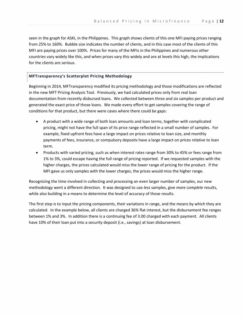
extreme variation in their pricing maps, as Figure 1: Full APR for ASKI
B a l a n c e d P r i c i n g i n M i c r o f i n a n c e P a g e | 12
seen in the graph for ASKI, in the Philippines. This graph shows clients of this one MFI paying prices ranging
from 25% to 160%. Bubble size indicates the number of clients, and in this case most of the clients of this
MFI are paying prices over 100%. Prices for many of the MFIs in the Philippines and numerous other
countries vary widely like this, and when prices vary this widely and are at levels this high, the implications
for the clients are serious.
MFTransparency's Scatterplot Pricing Methodology
Beginning in 2014, MFTransparency modified its pricing methodology and those modifications are reflected
in the new MFT Pricing Analysis Tool. Previously, we had calculated prices only from real loan
documentation from recently disbursed loans. We collected between three and six samples per product and
generated the exact price of those loans. We made every effort to get samples covering the range of
conditions for that product, but there were cases where there could be gaps:
A product with a wide range of both loan amounts and loan terms, together with complicated
pricing, might not have the full span of its price range reflected in a small number of samples. For
example, fixed upfront fees have a large impact on prices relative to loan size, and monthly
payments of fees, insurance, or compulsory deposits have a large impact on prices relative to loan
term.
Products with varied pricing, such as when interest rates range from 30% to 45% or fees range from
1% to 3%, could escape having the full range of pricing reported. If we requested samples with the
higher charges, the prices calculated would miss the lower range of pricing for the product. If the
MFI gave us only samples with the lower charges, the prices would miss the higher range.
Recognizing the time involved in collecting and processing an even larger number of samples, our new
methodology went a different direction. It was designed to use less samples, give more complete results,
while also building in a means to determine the level of accuracy of those results.
The first step is to input the pricing components, their variations in range, and the means by which they are
calculated. In the example below, all clients are charged 36% flat interest, but the disbursement fee ranges
between 1% and 3%. In addition there is a continuing fee of 3.00 charged with each payment. All clients
have 10% of their loan put into a security deposit (i.e., savings) at loan disbursement.

B a l a n c e d P r i c i n g i n M i c r o f i n a n c e P a g e | 13
The next step (shown below) requires estimations of how the loans are spread out by loan amount and by
loan term. In this example, 10% of the loans are under P700, 20% are in the range of 700-1,400, and so on.
For loan terms, half the loans are 6 months and half are 9 months. These figures do not need to be precise.
Approximations still give very reliable results. The orange cells in the center of the left matrix show
estimates of how the 10,000 clients of this loan product are distributed, based on the percentages entered.
The matrix on the right side of the figure allows the analyst to pick a number of samples. In this case there
are 8 samples identified, and each sample has a specified loan amount and loan term specified by the
matrix.
The next section of the tool then auto-generates variations on the eight samples. In this case, there are
different fees charged, so the tool has created two variations for each sample, charging 1% to one variation

B a l a n c e d P r i c i n g i n M i c r o f i n a n c e P a g e | 14
and 3% in the other. The tool does allow the user to alter this, e.g., maybe loans under P.1000 always pay
3%, or maybe there are some loans that are charged 2%.
Once the modifications are entered, the tool then generates the prices of all sixteen samples, and they are
displayed in the pricing scatterplots. The graph below shows the pricing related to loan amount, but the
tool include a graph of pricing related to loan term, as well as numerous analysis tables for studying the
impact of the price components. In this example, we see that prices range from 80% to 140%, and the
prices follow the theoretical pricing curve.
To determine if these automatic price calculations are reliable, the analyst requests two real loan samples of
one of the products of the MFI. The analyst calculates the prices of those samples using the loan
documentation and compares those prices to the auto-generated price of a loan of the same amount and
term. If the prices differ, then there are either errors in the inputs or the MFI calculates interest or applies
fees differently than done in the software. If the prices are very close to the same, then the analyst can
assume that the data is entered properly and the MFI's procedures match standard procedures incorporated
into the software. The previous pricing methodology would request and process up to 24 repayment

B a l a n c e d P r i c i n g i n M i c r o f i n a n c e P a g e | 15
schedules for an MFI with four products; the new approach achieves more comprehensive pricing
information while processing just 2 repayment schedules.
A case study example from Bolivia
For the remainder of this analysis in Part II, we will return to the example of Bolivia and will use pricing and
expense figures from one of the MFIs in Bolivia that has relatively small loans and charges relatively higher
prices. Inputting their data into the Pricing Analysis Tool yields the following pricing scatterplot, with
Product 1 clients paying between 33% and 36% on smaller loans, and Product 2 clients paying between 12%
and 24% on larger loans, with the higher prices falling on the smaller loans.
Part II: Dissecting MFI expenses
Our next step is to explore how we can break apart aggregate expense figures into expenses related to
different loan sizes. We've seen in Part I that MFIs targeting different levels of the market have an
Operating Cost Ratio that follows a curve. Let's start with a straightforward way to see why there is an
operational cost curve (using simplified figures so the math is crystal clear).

B a l a n c e d P r i c i n g i n M i c r o f i n a n c e P a g e | 16
Why is there a curve for the Operating Cost Ratio?
Assume your MFI generally makes loans of
$500 for 12 months, and when you evaluate
the costs your institution makes to disburse
and monitor the loan, they total to $50.
That gives you an Operating Cost Ratio of
10% and you are congratulated for excellent
management, resulting in high efficiency.
But the same evaluators encourage you
to make smaller loans so that you are
including more of the needy. So you
decide to start providing loans of $250.
You have your loan officers spend the
same amount of time with these
clients, and you pay the loan officers
the same wage. Therefore, your expenses stay at $50 per loan, and that results in an operating cost ratio of
20%, twice as high as the larger loans. The evaluators return, and they question why your efficiency has
gotten dramatically worse.
Even though you are now giving
smaller loans, there are other MFIs
giving much smaller loans of $100. You
know if you are to go into this market,
you'll need to get your cost per client
down. You'll need to spend less time
with the clients, and you may even
need to pay these loan officers a lower wage than the other loan officers. You cut your costs per loan from
$50 to $30, a dramatic improvement. But when compared to the loan size of $100, your operating cost ratio
continues to escalate, reaching 30%. Your managerial skills are brought into question.
Map out this data, and you'll find the curve we saw earlier. MFIs with smaller average loan balances have
higher operating cost ratios. What we are seeing with this analysis, however, is something very important
— different loans inside the same MFI have different operating cost ratios. This has implications for the
prices we charge on our loans, and that is the next step in our analysis.
Allocating expenses by loan size
Let’s go back to the BancoSol graph and add their average Operating Cost figure of 11% correlated with their
average loan amount of 5,000, directly under their portfolio yield of 20%.

B a l a n c e d P r i c i n g i n M i c r o f i n a n c e P a g e | 17
We have seen in Part I of the expense analysis that not every loan of BancoSol has an operating cost ratio.
This figure of 11% is also a global average that masks the impact of the range of loan amounts, like the
portfolio yield masks the range of prices paid by clients.
We know from MFT's work that we can generate the range of loan prices by generating the APRs of different
samples of the different products. Can we create a reasonable estimate of the costs related to each of these
loan samples? Yes, we can, and it doesn't even take much additional data or additional work. The process
uses the Balanced Pricing Tool feature of the MFTransparency Pricing Analysis Tool.
To demonstrate, we will generate figures for the same MFI whose pricing scatterplot was shown on a
previous page. The first section of the Balanced Pricing Tool assembles information entered during pricing
calculations -- total number of clients, total portfolio, and smallest and largest loan sizes from the micro loan
products. Using exchange rate and GNI information for the country, this section generates some useful
ratios.
The next section on the worksheet is the only area requiring any input. All other information in the tables
and graphs is generated automatically. The first column allows input of the ratios we discussed earlier, with
the Operating Expense Ratio split up into two parts — personnel expense and admin expense. These figures
must all be based on loan portfolio, as indicated in the column title.

B a l a n c e d P r i c i n g i n M i c r o f i n a n c e P a g e | 18
They are then applied to the portfolio figure in the previous figure to generate an approximation of the
budget in both national currency and USD. The middle section then divides these figures by the total
number of clients to get costs per client for each expense area. In this example, personnel expenses are
US$78 per client and admin is $31, for a total operating expense of $109. To these are added $47 of
financial expense and $31 of loan loss, to give total expenses of $187 per client. As indicated in the earlier
table, the average balance per client is $780, so this gives a total cost ratio of $187 / $780, or 24%.
However, this is the global average and is true only for that client who might get a loan with an average
balance of $780. We need to do better than this. The columns on the right side of that table above allow
you to decide how to allocate costs for different loan sizes using the grey cells that contain dropdowns with
two choices - by client, or by portfolio. The personnel expenses of $78 (or 527 in national currency) are
likely to remain the same regardless of loan size. Choosing "by client" means that BOL 527 will be applied to
each loan. Admin expenses are also very likely to be correlated by client rather than by portfolio. However,
financial expenses and loan loss, as we saw earlier, are constant percentages, independent of loan size.
They are highly correlated to portfolio. In this example, they will be assigned at the rates of 6% and 4%.
The remaining tables and graphs of the worksheet are now fully generated and can be reviewed. First, we
need to understand the overall structure of the table on the next page. The columns are related to different
loan amounts, expressed as a percentage of GNI/capita. There are more columns concentrated on the
smaller percentages — 5%, 10%, 18%, and 25% — because this is where the curve is found. On the right
side of the table are columns for 100%, 150%, 200% and 300%. As we will see, even with these large gaps of
up to 100%, the figures are quite flat. There are two colors of columns — blue columns contain information
directly linked to the segments identified on the pricing pages of the software, while green columns are
extrapolations, averaging the information in the blue columns to either side.

B a l a n c e d P r i c i n g i n M i c r o f i n a n c e P a g e | 19
The row titled Covered by this MFI indicates if the
MFI has any loans in that portion of the market.
Figures are then generated for these columns. In
Costs per Loan, figures are applied as defined earlier.
Personnel Expenses are 527 for each loan and Admin
Expenses are 211. However, Financial Expenses are
calculated as 6% of the average loan balance, so the
figure varies in each column, as does Net Impairment
Loss, calculated at 4%. Total Expenses per Loan range
from 794 to 2,682.
The figures in Costs per Loan are then converted to
Cost Ratios, dividing the amounts by the average
balance for each loan. Personnel and Admin
Expenses vary dramatically, while Financial and Loan
Loss Expenses are a constant percentage because
they were calculated using a constant percentage.
The information from the tables is now shown
graphically. The first graph shows each cost
component relative to the loan amount as a
percentage of GNI/Capita. The orange triangle
represents the 14% figure that is the average
Operating Expense Ratio for the institution for the
average loan balance of 75% of GNI per capita.
Financial expense and Net Impairment Loss are both
very small and flat. The Operating Expense Ratio
creates a dramatic curve.

B a l a n c e d P r i c i n g i n M i c r o f i n a n c e P a g e | 20
Could this be true? Based on the assumptions that the MFI spends 737 in operating costs per client over
the course of an entire year, it is true. If the MFI does have a means to spend less money (i.e., spend less
staff time) on clients with the very smallest loans, then the cost per client could have some variation in it.
This is, in fact, what generally happens with group lending, as clients are grouped to reduce the time spent
with each client. However, the product-specific OERs would only vary if the MFI had two products of
significant scale, each using different lending methodologies. If the major products use similar
methodologies, there would be no difference; if products have different methodologies but one of them has
over 70% of the total portfolio, the impact on the calculations is likely to be marginal. I do plan to add this
option into the next version of the tool.
In the graph above, the OER line is flat for loans above 150% GNI per capita. It transitions to a sloped line
from 150% to about 75%. It then increasingly becomes a steeper line that approximates a vertical line.
These figures match those indicated in MFT's paper from 2011 paper Is Transparency Enough? What is Fair
and Ethical in Pricing? The figures also reflect the reality that the cost curve must be an asymptotic curve
where the OER approaches infinity as the loan amount approaches zero.
In conclusion: For those MFIs providing loans under 50% of GNI/capita to at least some of its clientele, the
OER of these loans are very high, even scarily high. If these loans are to cover their costs, the prices will
need to be equally as high, or the subsidies need to come from elsewhere.
Part II: Comparing Income and Expense, Client-by-Client
We now have income and expense figures for each size of loan offered by this MFI, and we can compare
them. The next graph shows two lines – the Total Expense Ratio, which is a dramatic curve, and the
Weighted Average Price, calculated by using the distribution of clients by loan size and the prices charged on
each size loan.

B a l a n c e d P r i c i n g i n M i c r o f i n a n c e P a g e | 21
As expected, the smallest loans are not priced high enough to cover their full costs and the MFI therefore
loses money on these loans. However, once loan sizes exceed 50% GNI per capita, their price exceeds costs
and the MFI generates profit. It is important to recognize that these profit and loss figures are per unit of
portfolio, so this information needs to be correlated to the amount of portfolio in each segment to
determine the overall financial performance of the MFI. In other words, if the amount of portfolio in loans
under 25% of GNI per capita is quite small, the MFI has modest losses. We’ll do these calculations shortly.
Before doing those calculations, we can use the per product price calculations to evaluate the performance
of each product. This next graph shows that Prod 1 has a consistently higher price than Prod 2, staying very
close to 35% for loans ranging from 5% of GNI to 200% of GNI. As the cost of the larger loans drops much
lower than the price, the MFI generates substantial profits on these larger loans in Prod 1.

B a l a n c e d P r i c i n g i n M i c r o f i n a n c e P a g e | 22
Prod 2 has a much lower price, as
shown by the red line. On the
smallest amounts (around 40% GNI),
the price is about 24%. The price
drops continually, reaching about 12%
on the largest loans at 300% of GNI
per capita. In other words, this
product sees some losses on the
smallest loans in Prod 2, and likely
doesn’t generate enough profit on the
largest loans to offset these losses.
Finally, the detailed table to the right
shows the APR for each loan product
for each loan amount and then
calculates the spread, as the
difference between the Total Expense
Ratio and the APR. These figures are
applied to the average balance per
client figures to determine income,
expense, and net result for clients at
each loan amount. These figures are
then multiplied by the number of
clients at each loan amount to
generate aggregate profit/loss figures.
The very bottom rows tally the
cumulative profit/loss figures for each
product and the institution.

B a l a n c e d P r i c i n g i n M i c r o f i n a n c e P a g e | 23
When an MFI has activity on the curve, there are likely significant cross-subsidies
Everything we see in this analysis was generated by applying standard business logic, but the results surprise
us because they don’t reflect what we see in standard business. As we find so often in microfinance, we can
use our tools from business school, but we need to look at the results with open eyes and not apply our
judgements we learned in business school. Microfinance is a different world from traditional finance when
you reach the steep portion of the curve.
Cross-subsidies make sense in business logic, but we don’t generally see them so pronounced in traditional
finance because nearly all of the activity is on the right side of these graphs, on the flat part of the curve.
Credit card financing deals with smaller amounts, and that is one reason it is higher priced. Some of
microfinance is on the flat part of the expense line, e.g., loans over 200% of GNI per capita (giving and
average loan balance of 100% of GNI per capita). Some MFIs work in this area, as we saw in Bolivia, and
some MFIs work exclusively in this area, such as ProCredit.
The graph below shows activity for MFIs like ProCredit, who work in the “safe area.” Except for the smallest
loans at 100% of GNI, every loan is profitable, and most of them are profitable to approximately the same
degree – the results of a flat price line and flattish cost line. Although this MFI is still meeting a market need,
it would likely receive criticism from others in the industry for not making small enough loans.
Thus, another strategy is to make the very small loans but to also cover a broad range of loan sizes, as do
MFIs such as Banco Sol. The next graph shows how low prices can be charged to every client, and the losses
coming from the very smallest loans are offset by moderate profit levels from the largest loans. Cross-
subsidies enable this strategy of working with the poorest, offering them low, affordable prices, and still
being profitable.

B a l a n c e d P r i c i n g i n M i c r o f i n a n c e P a g e | 24
The last graph shows the approach of MFIs such as Banco Compartamos, or many of the MFIs in Mexico and
Philippines. In these two countries, MFIs offer only extremely small loans, with the largest loan size being on
the order of 30% of GNI per capita. All of their activity is on the steepest part of the curve. Even with well-
designed structures and staff working efficiently, the operating cost ratios are extremely high. Even when
charging high prices, the smallest loans still lose money. As there is not a lot of portfolio in larger loan sizes,
the MFI has no place to generate profits to offset the losses than to continue to charge the very high prices
on the somewhat larger loans.
Looking again at the pricing scatterplot for the MFI with two products. One product is targeted to smaller
loan sizes and is higher priced. The other product is larger loan amounts at a much lower price. However,
there is a significant overlap of identical loan amounts for the two products, at very different prices.
Consider a loan of $2,000, available in both products; it has a price of 34% for Product 1 and 20% for Product
2. Product 1 is a group product and should therefore arguably have lower costs than Product 2, which is an
individual product, but it has a much higher price. There appears to be some cross-subsidization, and the

B a l a n c e d P r i c i n g i n M i c r o f i n a n c e P a g e | 25
Balanced Pricing calculations we generated indicate the same. Enabled by this analysis, management could
revise the coverage and prices of the two loan products to achieve better balance.
CONCLUSION
Cross-subsidies do take place in microfinance, and very often to a significant degree. We haven’t recognized
that reality, we haven’t had a means to measure that reality, and we haven’t have criteria to judge that
reality. Is it responsible practice to subsidize $200 loans with profits from the larger $2,000 loans? If so, to
what degree? Perhaps more troubling, is it responsible practice to subsidize $2,000 loans with profits made
from the smaller $200 loans? Should the poor subsidize the less poor? Or is all subsidy to be avoided? If so,
should responsible MFIs charge 300% on their $100 loans, 100% on the $200 loans, and 20% on the $2,000
loans?
The approach presented in this paper can help us advance discussion on these issues. By improving our
understanding of how expenses and prices form a curve, we can improve our definitions of responsible
practice and managers can make wiser decisions that achieve more balance in what may currently be a
chaotic situation hiding behind an overall RoA figure. Financial institutions working near the edges of
financial inclusion operate in an environment where different interpretations of financial ratios apply and
where benchmarks shift quickly. There is a reason why conventional finance chose not to extend this
deeply, and microfinance needs to be fully cognizant of this different environment.
Being a Balanced Business goes beyond the obligation "don't break any laws". A balanced business respects
its clients and doesn't take advantage of them. A balanced business strives to balance its own needs with
the needs of its client base. A balanced business that respects its clients will find the approach presented in
this paper to be intellectually stimulating and provide a useful new perspective to use as it makes decisions
about who it works with, the design of its products, and the prices of those products. As Kant said, "Always
recognize that human individuals are ends, and do not use them as means to your end."
Recommended