University of Southern Queensland
Faculty of Engineering and Surveying
Autonomous Unmanned Aerial Surveillance
Vehicle – Autonomous Control and Flight
Dynamics
A dissertation submitted by
Craig Andrew LITTLETON
In fulfilment of the requirements of
Courses ENG4111 and 4112 – Research Project
Towards the degree of
Bachelor of Engineering Electrical and Electronic
Bachelor of Business Operations and Logistics Management
Submitted: October 2005

i
Abstract
The field of autonomous UAV research and development is a rapidly expanding
sector of engineering. Technological advances in aircraft design, solid state
devices, communications and battery technology have allowed for a shift in UAV
technology from purely militarised applications towards lower cost general
aviation purposes. In short, it appears that autonomous UAV technology is the
future for aviation as we know it.
The overall project (when combined with “Navigation and User Interface”, Knox
2005) seeked to develop a low cost, fixed wing UAV system to conduct specific
flight path surveillance over a pre-determined waypoint path. This particular
section of the project focussed on the task of controlling the stability of the
aircraft during its mission. The basis for the autonomous control of the UAV
system lies within the analysis of aircraft flight dynamics. From the dynamics of
flight, it is possible to design a control system based on either conventional
control techniques, or more simply an “observe and correct” system.
Whilst it is recommended for future work that a more conventional approach be
taken to this AFCS design, an “observe and correct” approach was adopted for
the purposes of this project. This system automatically corrected for heading
errors via an outer loop function, and maintained aircraft stability, by monitoring
the pitch and roll characteristics of the aircraft, via an inner loop function. This
process was achieved through the use of a MC912D60A HC12 microcontroller
for all embedded computing requirements and a single ADXL213 accelerometer
module for pitch and roll measurement. Heading information was passed to the
AFCS from “Navigation and User Interface” (Knox, 2005).
Whilst a prototype UAV system was unable to be developed and therefore final
flight testing was unable to be conducted, this project has provided a strong base
for future work in this area. The flight dynamics analysis and simulation methods
outlined in this dissertation will provide a useful starting point for any future
AFCS design. Also, program development such as Rx/Tx remote signal routing

ii
through the HC12, accelerometer signal decoding, and servo motor control, are
fundamental to any control method utilising similar components and were all
tested and verified, hence providing a solid programming base for any future
work.
This project encountered numerous limitations such as budgetary constraints and
unavailability of crucial information (in the form of stability data for a model
aircraft). If these limitations can be overcome in the future, this project has
provided sound guidance and a solid foundation towards the development of a
fully functioning prototype autonomous UAV system.

iii
University of Southern Queensland
Faculty of Engineering and Surveying
Limitations of Use
The Council of the University of Southern Queensland, its Faculty of
Engineering and Surveying, and the staff of the University of Southern
Queensland, do not accept any responsibility for the truth, accuracy or
completeness of material contained within or associated with this dissertation.
Persons using all or any part of this material do so at their own risk, and not at
the risk of the Council of the University of Southern Queensland, its Faculty of
Engineering and Surveying or the staff of the University of Southern
Queensland.
This dissertation reports an educational exercise and has no purpose or validity
beyond this exercise. The sole purpose of the course pair entitled "Research
Project" is to contribute to the overall education within the student’s chosen
degree programme. This document, the associated hardware, software, drawings,
and other material set out in the associated appendices should not be used for any
other purpose: if they are so used, it is entirely at the risk of the user.
Prof G Baker
Dean
Faculty of Engineering and Surveying
ENG4111 & ENG4112 Research Project

iv
Certification
I certify that the ideas, designs and experimental work, results, analyses and
conclusions set out in this dissertation are entirely my own effort, except where
otherwise indicated and acknowledged.
I further certify that the work is original and has not been previously submitted
for assessment in any other course or institution, except where specifically stated.
Craig Andrew LITTLETON
Student Number: Q1221674
………………………………………………
Signature
………………………………………………
Date

v
Acknowledgements
The initial concept for this project came from Mr Terry Byrne from the Faculty
of Engineering and Surveying, and if it wasn’t for his vision this project would
not have been undertaken. So thanks must first go to Terry for the idea as well as
his continued technical support and suggestions throughout the year. Thankyou
also to my supervisor Mr Mark Phythian for the guidance and expertise he has
provided throughout the course of this project, without his input this project
would have been significantly more difficult.
Also to my colleague Ms Soz Knox who undertook the other half of this very
large (and very technically demanding!) project. Even though we didn’t make it
to a final prototyping stage (an aircraft would have been helpful here!), and
therefore never actually got to see our creation fly, I have enjoyed working on
this project with you and I know that you have enjoyed the challenge also. I hope
that the end result of the combined project will provide a solid foundation for
future research.
The concept of the UAV is both exciting and challenging. I suggest to anyone
considering a final year project to take up the challenge and to continue
development. Hopefully in future years someone will be able to develop a
working prototype UAV and hopefully that student/students will take pride in
their achievements and exhibit the same enthusiasm that I have felt for this
project.

vi
Table of Contents
Abstract i
Disclaimer iii
Certification iv
Acknowledgements v
Table of Contents vi
List of Figures ix
List of Equations xi
List of Tables xii
Nomenclature xiii
Chapter 1 Introduction
1.1 Project Background 1
1.2 Project Aims and Objectives 2
1.3 Project Methodology 3
1.4 Legal Requirements of UAV systems 4
1.5 Dissertation Overview 8
Chapter 2 Dynamics of Flight
2.1 Axis Referencing 11
2.2 Euler’s Equations of Motion 13
2.3 Small Disturbance Theory 14
2.4 Simplification 17
2.5 Equations of Longitudinal Motion 18
2.6 Equations of Lateral Motion 19
Chapter 3 Flight Controller Development
3.1 Flight Control Theory 21
3.2 State Space Representation 23
3.2.1 Longitudinal System 24
3.2.2 Lateral System 26

vii
3.3 Transfer Function Representation 28
3.3.1 Longitudinal Transfer Function and Stability 28
3.3.2 Lateral Transfer Function and Stability 30
3.4 Controllability and Observability 31
Chapter 4 Continuous-Time System Simulations
4.1 Root Locus 35
4.1.1 Longitudinal 35
4.1.2 Lateral 36
4.2 Bode Plots 37
4.2.1 Longitudinal 37
4.2.2 Lateral 39
4.3 Longitudinal System Responses 39
4.3.1 Step Response 39
4.3.2 Impulse Response 41
4.4 Lateral System Responses 43
4.4.1 Step Response 43
4.4.2 Impulse Response 44
Chapter 5 Discrete-Time System Simulations
5.1 System Discretization 46
5.2 Longitudinal System Responses 50
5.2.1 Step Response 50
5.2.2 Impulse Response 51
5.3 Lateral System Responses 53
5.3.1 Step Response 53
5.3.2 Impulse Response 54
Chapter 6 Hardware Selection and Implementation
6.1 Microcontroller 57
6.2 Aircraft 58
6.2.1 Transmit/Receive Remote Signal Routing 59
6.2.2 Servo Motor Control 60
6.3 Sensors 62

viii
6.3.1 Accelerometer 63
6.4 Manual Handover/System Monitoring 66
Chapter 7 Intuitive Control and Pre-Flight Testing
7.1 Intuitive Control versus Conventional Control 69
7.2 The Intuitive Approach 69
7.3 Roll Constraints 72
7.4 Primary Control Algorithm Testing 73
7.4.1 Hardware Setup 74
7.4.2 Software Setup 77
7.4.3 Test Results 78
7.5 Remote Tx/Rx Signal Routing Algorithm Testing 79
7.6 Future Testing 81
7.6.1 Primary Control Algorithm 81
7.6.2 Manual Handover and System Monitoring 81
Chapter 8 Discussion and Conclusions
8.1 Overall System Analysis 83
8.2 Limitations Encountered 85
8.3 Recommendations for Future Work 87
8.4 Autonomous Take-off and Landing Feasibility 88
8.5 Final Word 91
References 92
Appendix A – Project Specification 94
Appendix B – Exert from Civil Aviation Safety Regulations 1998 96
Appendix C – MATLAB Simulation Files 104
Appendix D - MC912D60A HC12 Microcontroller Assembly
Language Control Algorithms 109
Appendix E - Technical Specifications of SensComp 6500 Series
Ranging Module 126
ix
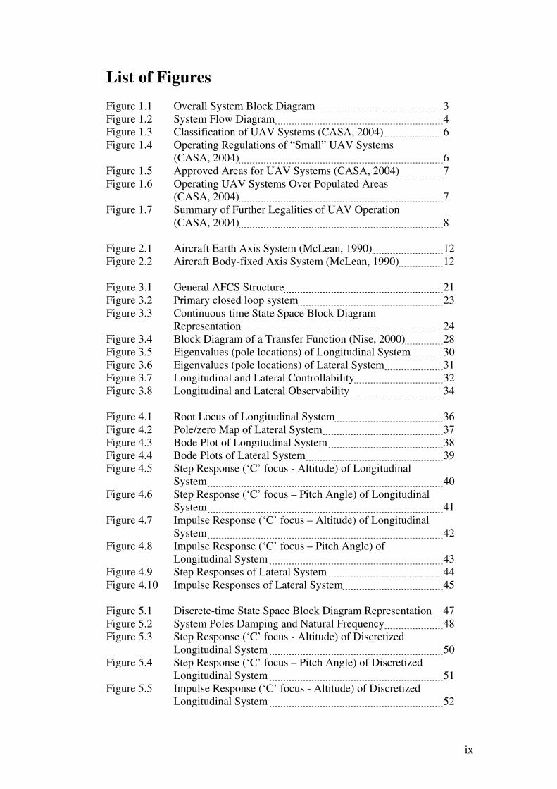
List of Figures
Figure 1.1 Overall System Block Diagram 3
Figure 1.2 System Flow Diagram 4
Figure 1.3 Classification of UAV Systems (CASA, 2004) 6
Figure 1.4 Operating Regulations of “Small” UAV Systems
(CASA, 2004) 6
Figure 1.5 Approved Areas for UAV Systems (CASA, 2004) 7
Figure 1.6 Operating UAV Systems Over Populated Areas
(CASA, 2004) 7
Figure 1.7 Summary of Further Legalities of UAV Operation
(CASA, 2004) 8
Figure 2.1 Aircraft Earth Axis System (McLean, 1990) 12
Figure 2.2 Aircraft Body-fixed Axis System (McLean, 1990) 12
Figure 3.1 General AFCS Structure 21
Figure 3.2 Primary closed loop system 23
Figure 3.3 Continuous-time State Space Block Diagram
Representation 24
Figure 3.4 Block Diagram of a Transfer Function (Nise, 2000) 28
Figure 3.5 Eigenvalues (pole locations) of Longitudinal System 30
Figure 3.6 Eigenvalues (pole locations) of Lateral System 31
Figure 3.7 Longitudinal and Lateral Controllability 32
Figure 3.8 Longitudinal and Lateral Observability 34
Figure 4.1 Root Locus of Longitudinal System 36
Figure 4.2 Pole/zero Map of Lateral System 37
Figure 4.3 Bode Plot of Longitudinal System 38
Figure 4.4 Bode Plots of Lateral System 39
Figure 4.5 Step Response (‘C’ focus - Altitude) of Longitudinal
System 40
Figure 4.6 Step Response (‘C’ focus – Pitch Angle) of Longitudinal
System 41
Figure 4.7 Impulse Response (‘C’ focus – Altitude) of Longitudinal
System 42
Figure 4.8 Impulse Response (‘C’ focus – Pitch Angle) of
Longitudinal System 43
Figure 4.9 Step Responses of Lateral System 44
Figure 4.10 Impulse Responses of Lateral System 45
Figure 5.1 Discrete-time State Space Block Diagram Representation 47
Figure 5.2 System Poles Damping and Natural Frequency 48
Figure 5.3 Step Response (‘C’ focus - Altitude) of Discretized
Longitudinal System 50
Figure 5.4 Step Response (‘C’ focus – Pitch Angle) of Discretized
Longitudinal System 51
Figure 5.5 Impulse Response (‘C’ focus - Altitude) of Discretized
Longitudinal System 52

x
Figure 5.6 Impulse Response (‘C’ focus – Pitch Angle) of
Discretized Longitudinal System 52
Figure 5.7 Step Response of Lateral System (Input – Rudder) 53
Figure 5.8 Step Response of Lateral System (Input – Aileron) 54
Figure 5.9 Impulse Response of Lateral System (Input –Rudder) 55
Figure 5.10 Impulse Response of Lateral System (Input – Aileron) 56
Figure 6.1 Tx/Rx Routing Through the HC12 60
Figure 6.2 Servo Control Theory 61
Figure 6.3 Servo Limitations 62
Figure 6.4 PWM Decoding Theory 64
Figure 6.5 Accelerometer Pitch and Roll Error Measurement
Characteristics 65
Figure 6.6 Block Diagram of Proposed Hardware 67
Figure 6.7 555 Timer Monostable Circuit Arrangement 68
Figure 7.1 Primary Closed Loop System 70
Figure 7.2 Process Flow of Primary Control Algorithm 71
Figure 7.3 Accelerometer Testing Setup 75
Figure 7.4 Servo Motor Testing Setup 75
Figure 7.5 Overall Test Setup 76
Figure 7.6 Screen Shot of TwinPEEKs Monitor Program 77
Figure 7.7 Software Flow Chart of Primary Control Algorithm 78
Figure 7.8 CRO Screenshot of Tx/Rx Algorithm Testing 79
Figure 7.9 CRO Screenshot with Shortened Time Scale 80
Figure 8.1 Conventional Control Approach 86
Figure 8.2 Take-off Sequence 89
Figure 8.3 Landing Sequence 90
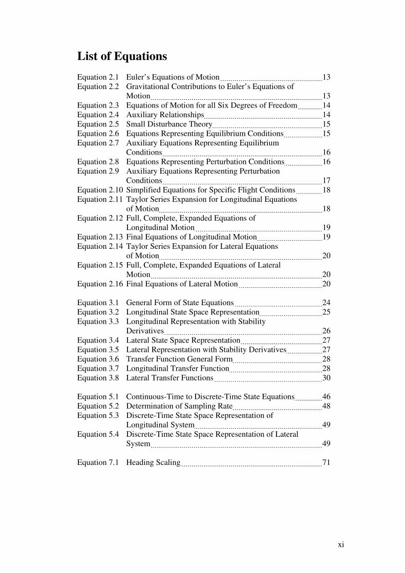
xi
List of Equations
Equation 2.1 Euler’s Equations of Motion 13
Equation 2.2 Gravitational Contributions to Euler’s Equations of
Motion 13
Equation 2.3 Equations of Motion for all Six Degrees of Freedom 14
Equation 2.4 Auxiliary Relationships 14
Equation 2.5 Small Disturbance Theory 15
Equation 2.6 Equations Representing Equilibrium Conditions 15
Equation 2.7 Auxiliary Equations Representing Equilibrium
Conditions 16
Equation 2.8 Equations Representing Perturbation Conditions 16
Equation 2.9 Auxiliary Equations Representing Perturbation
Conditions 17
Equation 2.10 Simplified Equations for Specific Flight Conditions 18
Equation 2.11 Taylor Series Expansion for Longitudinal Equations
of Motion 18
Equation 2.12 Full, Complete, Expanded Equations of
Longitudinal Motion 19
Equation 2.13 Final Equations of Longitudinal Motion 19
Equation 2.14 Taylor Series Expansion for Lateral Equations
of Motion 20
Equation 2.15 Full, Complete, Expanded Equations of Lateral
Motion 20
Equation 2.16 Final Equations of Lateral Motion 20
Equation 3.1 General Form of State Equations 24
Equation 3.2 Longitudinal State Space Representation 25
Equation 3.3 Longitudinal Representation with Stability
Derivatives 26
Equation 3.4 Lateral State Space Representation 27
Equation 3.5 Lateral Representation with Stability Derivatives 27
Equation 3.6 Transfer Function General Form 28
Equation 3.7 Longitudinal Transfer Function 28
Equation 3.8 Lateral Transfer Functions 30
Equation 5.1 Continuous-Time to Discrete-Time State Equations 46
Equation 5.2 Determination of Sampling Rate 48
Equation 5.3 Discrete-Time State Space Representation of
Longitudinal System 49
Equation 5.4 Discrete-Time State Space Representation of Lateral
System 49
Equation 7.1 Heading Scaling 71

xii
List of Tables
Table 6.1 MC912D60A Technical Specifications (Motorola,
2000; Elektronikladen, 2005) 58
Table 6.2 Aircraft Technical Specifications 59
Table 6.3 Sensor Information Summary 63
Table 7.1 Scaled Heading Examples 72
Table 7.2 Roll Constraint Guide 73
Table 7.3 Expected Errors for Constraint Limits 73

xiii
Nomenclature
UAV Unmanned Aerial Vehicle
MAV Micro Aerial Vehicle
Tx Transmit
Rx Receive
GPS Global Positioning System
XE X-axis of the earth axis system
YE Y-axis of the earth axis system
ZE Z-axis of the earth axis system
XB X-axis of the aircraft (Body-fixed axis system)
YB Y-axis of the aircraft (Body-fixed axis system)
ZB Z-axis of the aircraft (Body-fixed axis system)
U Forward velocity
V Side velocity
R Yawing velocity
L Rolling moment
M Pitching moment
N Yawing moment
P Roll angular velocity
Q Pitch angular velocity
R Yaw angular velocity
Φ Roll angle
Θ Pitch angle
Ψ Yaw angle
α Angle of attack
β Side slip angle of attack
g Acceleration due to gravity – 9.81 m.s-2
m Mass of an object
VT Total velocity vector
δe Elevator deflection angle
δa Aileron deflection angle
δr Rudder deflection angle
AFCS Automatic Flight Control System

xiv
A State matrix
B Driving matrix
C Output matrix
D Feed-forward matrix
K State feedback matrix
x State vector
u Control vector
y Output vector
SISO Single-input, Single-output system
MIMO Multiple-input, Multiple-output system
CM Controllability matrix
OM Observability matrix
dB Decibels
Γ Discrete driving matrix
Φ Discrete state matrix
ωo Highest frequency component in a signal (Nyquist frequency)
ωs Sampling frequency
I Identity matrix
k Sample instant
ZOH Zero-order-hold
Ts Sample time
PWM Pulse Width Modulation
IC Input Capture or Integrated circuit
OC Output Compare
RTI Real-time interrupt
PCB Printed circuit board
MSB Most Significant Bit
CRO Cathode Ray Oscilloscope
CASA Civil Aviation Safety Authority
CASR Civil Aviation Safety Regulations act
AGL Above Ground Level

Chapter 1 - Introduction
1
Chapter 1 Introduction
1.1 Project Background
The concept of the Unmanned Aerial Vehicle (UAV) is not a new concept. These
aircraft systems, capable of autonomous or semi-autonomous flight (or a
combination of the two), have been in operation since World War II. These
unpiloted aircraft (or ‘drones’ as they were known at the time) were originally
developed as targets for anti-aircraft gunnery training (Goebel, 2005). Since then
recent advances in communications, solid state devices and battery technology
(Beard et al, 2003) have allowed small, low-cost, fixed wing UAV systems to be
implemented for applications such as:
• Natural disaster monitoring and remediation
• Traffic and environmental monitoring
• Surveillance
• Security and law enforcement
• Terrain mapping (Innovations Report, 2004)
Whilst many of these applications are based on high cost systems, as indicated by
Beard et al (2003), there has been a recent shift towards research into more low
cost, Micro Aerial Vehicle (MAV) solutions. In recent years this research has
been common at a University level and a number of these low cost MAV systems
have been developed and refined throughout the world.
Chapter 1 - Introduction
2
A recent undergraduate project conducted at the University of Southern
Queensland attempted to develop a low cost autonomous aircraft system (Keeffe,
2003). Straight level flight was achieved; however the ability to fly a
predetermined flight path and gather useful information at predetermined points
(in the form of digital photographs) was not convincingly achieved. Keeffe (2003)
will provide the basis for this continuing project. Some aspects such as the flight
dynamics of the aircraft (which are universal) may be re-usable, whilst other
aspects such as control system design, sensor implementation and the overall
scope of the project will be built upon in an attempt to create a fully functioning,
low cost autonomous UAV system.
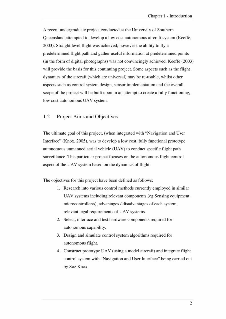
1.2 Project Aims and Objectives
The ultimate goal of this project, (when integrated with “Navigation and User
Interface” (Knox, 2005), was to develop a low cost, fully functional prototype
autonomous unmanned aerial vehicle (UAV) to conduct specific flight path
surveillance. This particular project focuses on the autonomous flight control
aspect of the UAV system based on the dynamics of flight.
The objectives for this project have been defined as follows:
1. Research into various control methods currently employed in similar
UAV systems including relevant components (eg Sensing equipment,
microcontroller/s), advantages / disadvantages of each system,
relevant legal requirements of UAV systems.
2. Select, interface and test hardware components required for
autonomous capability.
3. Design and simulate control system algorithms required for
autonomous flight.
4. Construct prototype UAV (using a model aircraft) and integrate flight
control system with “Navigation and User Interface” being carried out
by Soz Knox.
Chapter 1 - Introduction
3
As time permits:
1. Examine the viability of developing control algorithms for
autonomous take-off and landing sequences.
See appendix A for a more detailed Project Specification.
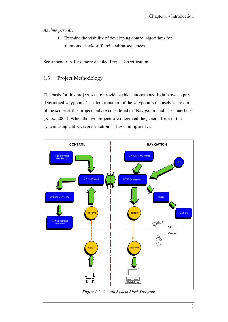
1.3 Project Methodology
The basis for this project was to provide stable, autonomous flight between pre-
determined waypoints. The determination of the waypoint’s themselves are out
of the scope of this project and are considered in “Navigation and User Interface”
(Knox, 2005). When the two projects are integrated the general form of the
system using a block representation is shown in figure 1.1.
Receive Transmit
Transmit Receive
CONTROL NAVIGATION
Accelerometer(Roll/Pitch)
System Monitoring
Control SurfaceActuators
HC12 (Control)
Compass (Heading)
HC12 (Navigation)
Trigger
Camera
GPS
Air
Ground
Figure 1.1: Overall System Block Diagram

Chapter 1 - Introduction
4
The “Control” side of figure 1.1 is the primary focus of this project. In its final
form it is intended that the UAV will operate as summarised by the flow diagram
in figure 1.2.
Figure 1.2: System Flow Diagram
Figure 1.2 shows that some user control is still required for both take-off and
landing cycles. If time permits the viability of introducing automatic take-off and
landing systems will be investigated, however in terms of implementation for this
project, based on initial research this issue appears to be quite complex and
therefore no attempts will be made to physically implement such a system.
There may also be room for possible expansion in the form of an “aided” flight
mode, whereby the user can control parameters such as thrust and/or altitude
(pitch) while the controller maintains the desired heading and maintains roll
stability. Exploration into this possibility will again only be conducted if all other
objectives are met.
1.4 Legal Requirements of UAV systems
Many of the legal aspects of UAV systems stem from common sense ethical
responsibilities. The following two aspects of ethical responsibility are exerts
from those set out by the Institution of Engineers Australia in 2000 Code of
Ethics (IEAUST, 2000). These ethical responsibilities are directed towards the
undertaking of any engineering practice.

Chapter 1 - Introduction
5
• Members shall place their responsibility for the welfare, health and
safety of the community before their responsibility to sectional or
private interests, or to other members.
• Members shall act with honour, integrity and dignity in order to merit the
trust of the community and the profession.
Basically these two formal responsibilities are directly applicable to the goal of
this project. The ‘welfare, health and safety of the community’ is of primary
importance to consider before any flight tests can be carried out. All systems
must be thoroughly tested by a combination of software simulation and on-
ground testing where possible. Flight tests should not be conducted until all
testing is passed. Aside from physical safety issues, acting with ‘honour,
integrity and dignity’ is an important constraint of the final objective. The
intended applications for these types of UAV systems are listed in section 1.1 of
this dissertation. With any surveillance application the issue of privacy becomes
important, and it must be made clear that it is not the goal of this project to
invade the privacy of the community by conducting surveillance of any private
property or unauthorized locations. For any future flight testing stage, the test
site needs to be chosen accordingly so as not to impose a threat to the
community’s right to privacy.
Issues such as these form the basis for legal requirements of UAV systems.
These requirements are extensively set out by the Civil Aviation Safety
Authority in the Civil Aviation Safety Regulations (CASR) act of 1998 (CASA,
2004), an exert of which appears in appendix B. This act covers all forms of
UAV platforms including; tethered balloons and kites, unmanned free balloons,
and UAV systems. The initial classification of a UAV system is broken into large,
small or micro, where:

Chapter 1 - Introduction
6
UAV means unmanned aircraft, other than a balloon or a kite;
A large UAV means any of the following:
(a) An unmanned airship with an envelope capacity greater than 100
cubic metres;
(b) An unmanned powered parachute with a launch mass greater than
150 kilograms;
(c) An unmanned aeroplane with a launch mass greater than 150
kilograms;
(d) An unmanned rotorcraft with a launch mass greater than 100
kilograms;
(e) An unmanned powered lift device with a launch mass greater than 100
kilograms.
A micro UAV means a UAV with a gross weight of 100 grams or less.
And a small UAV means a UAV that is neither a large UAV nor a micro UAV.
Figure 1.3: Classification of UAV Systems
(Adapted from Civil Aviation Safety Regulations act of 1998 (CASA, 2004))
Figure 1.3 indicates that for the purposes of this project the UAV system in
question will be under the “small” category. Operational regulations differ
slightly between the three system classes, a summary of the operating regulations
for a “small” UAV system are summarized in figure 1.4.
Operation near people
(1) A person must not operate a UAV within 30 metres of a person who is
not directly associated with the operation of the UAV.
(2) Subregulation (1) does not apply in relation to a person who stands
behind the UAV while it is taking off.
(3) Subregulation (1) also does not prevent the operation of a UAV
airship within 30 metres of a person if the airship approaches no closer to the
person than 10 metres horizontally and 30 feet vertically.
Where small UAVs may be operated
(1) A person may operate a small UAV outside an approved area only if:
(a) Where the UAV is operated above 400 feet AGL, the operator has CASA’s
approval to do so; and
(b) The UAV stays clear of populous areas.
Figure 1.4: Operating Regulations of “Small” UAV Systems
(Adapted from Civil Aviation Safety Regulations act of 1998 (CASA, 2004))
The “approved area” mentioned in the act is further defined as follows in figure
1.5.

Chapter 1 - Introduction
7
Approval of areas for operation of unmanned aircraft or rockets
(1) A person may apply to CASA for the approval of an area as an area
for the operation of:
(a) Unmanned aircraft generally, or a particular class of unmanned aircraft; or
(b) Rockets.
(2) For paragraph (1) (a), the classes of unmanned aircraft are:
(a) Tethered balloons and kites;
(b) Unmanned free balloons;
(c) UAVs;
(d) Model aircraft.
(3) In considering whether to approve an area for any of those purposes,
CASA must take into account the likely effect on the safety of air navigation of
the operation of unmanned aircraft in, or the launching of rockets in or over, the
area.
(4) An approval has effect from the time written notice of it is given to
the applicant, or a later day or day and time stated in the approval.
(5) An approval may be expressed to have effect for a particular period
(including a period of less than 1 day), or indefinitely.
(6) CASA may impose conditions on the approval in the interests of the
safety of air navigation.
(7) If CASA approves an area under subregulation (1), it must publish
details of the approval (including any condition) in NOTAM or on an
aeronautical chart.
(8) CASA may revoke the approval of an area, or change the conditions
that apply to such an approval, in the interests of the safety of air navigation
Figure 1.5: Approved Areas for UAV Systems
(Adapted from Civil Aviation Safety Regulations act of 1998 (CASA, 2004))
The CASR act also indicates guidelines for the operation of UAV systems in
populated areas. These are summarized in figure 1.6.
UAVs not to be operated over populous areas
(1) In this regulation: certificated UAV means a UAV for which a
certificate of airworthiness has been issued.
(2) A person must not operate a UAV that is not a certificated or does not
have approval of CASA over a populous area at a height less than the height
from which, if any of its components fails, it would be able to clear the area.
(3) In considering whether to give an approval under subregulation (2),
CASA must take into account:
(a) The degree of redundancy in the UAV’s critical systems; and
(b) Any fail-safe design characteristics of the UAV; and
(c) The security of its communications and navigation systems.
(4) Before giving an approval CASA must be satisfied that the UAV
operator will take proper precautions to prevent the proposed flight being
dangerous to people and property.
Figure 1.6: Operating UAV Systems over Populated Areas
(Adapted from Civil Aviation Safety Regulations act of 1998 (CASA, 2004))
Chapter 1 - Introduction
8
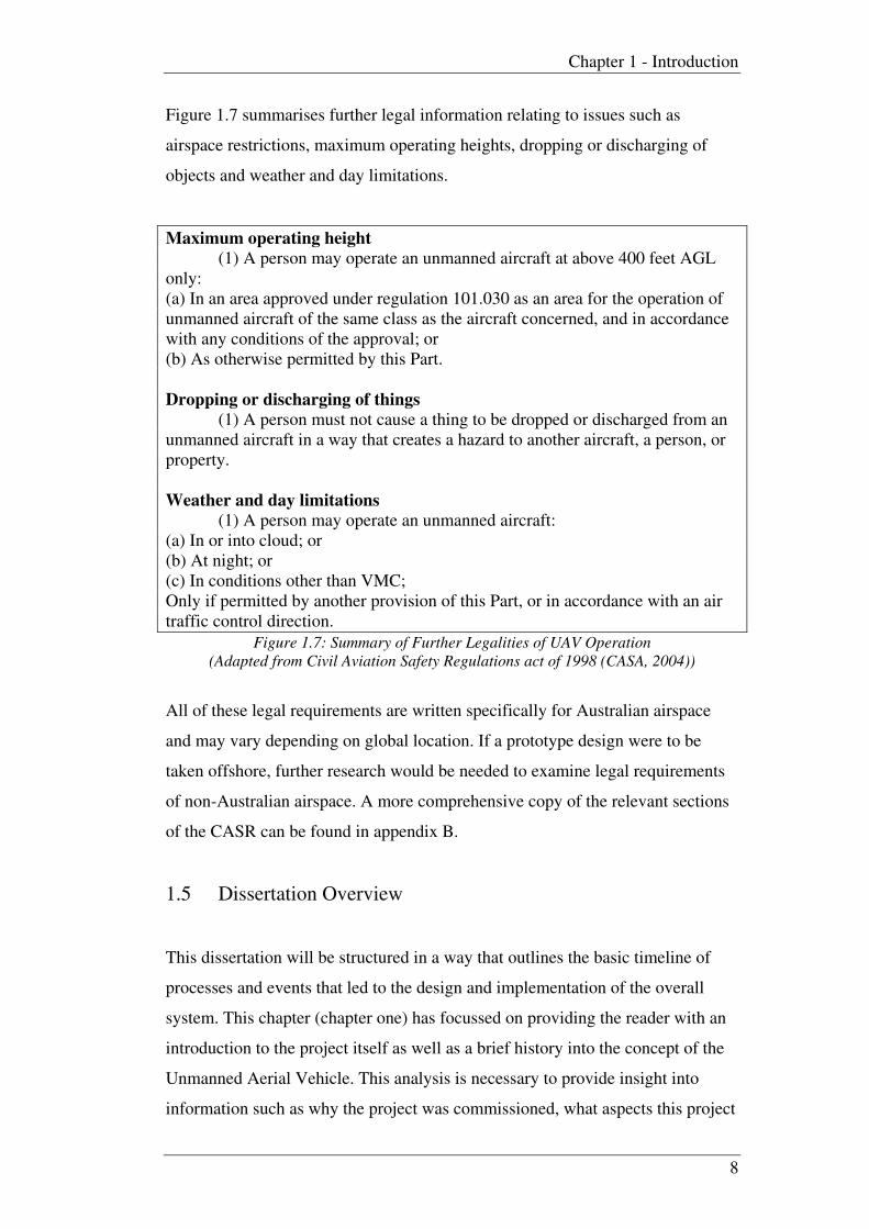
Figure 1.7 summarises further legal information relating to issues such as
airspace restrictions, maximum operating heights, dropping or discharging of
objects and weather and day limitations.
Maximum operating height
(1) A person may operate an unmanned aircraft at above 400 feet AGL
only:
(a) In an area approved under regulation 101.030 as an area for the operation of
unmanned aircraft of the same class as the aircraft concerned, and in accordance
with any conditions of the approval; or
(b) As otherwise permitted by this Part.
Dropping or discharging of things
(1) A person must not cause a thing to be dropped or discharged from an
unmanned aircraft in a way that creates a hazard to another aircraft, a person, or
property.
Weather and day limitations
(1) A person may operate an unmanned aircraft:
(a) In or into cloud; or
(b) At night; or
(c) In conditions other than VMC;
Only if permitted by another provision of this Part, or in accordance with an air
traffic control direction.
Figure 1.7: Summary of Further Legalities of UAV Operation
(Adapted from Civil Aviation Safety Regulations act of 1998 (CASA, 2004))
All of these legal requirements are written specifically for Australian airspace
and may vary depending on global location. If a prototype design were to be
taken offshore, further research would be needed to examine legal requirements
of non-Australian airspace. A more comprehensive copy of the relevant sections
of the CASR can be found in appendix B.
1.5 Dissertation Overview
This dissertation will be structured in a way that outlines the basic timeline of
processes and events that led to the design and implementation of the overall
system. This chapter (chapter one) has focussed on providing the reader with an
introduction to the project itself as well as a brief history into the concept of the
Unmanned Aerial Vehicle. This analysis is necessary to provide insight into
information such as why the project was commissioned, what aspects this project
Chapter 1 - Introduction
9
was to focus on, and how the overall system was expected to be designed and
integrated. Once this information is known to the reader, a detailed description of
the design and implementation stages can be delivered.
Chapter two was an essential starting point for any fixed wing aeroplane based
control system design. This chapter focuses on detailing the dynamic
characteristics of the aircraft, and more specifically the derivation of longitudinal
and lateral equations of motion. Chapter two forms the theoretical foundations
for the design of the automatic flight control system.
The development of the aircraft control theory itself is detailed in chapter three.
Chapter three links directly with the previous chapter and as mentioned, the
controller design depends primarily on the analysis of the dynamic characteristics
of the aircraft. Chapter three allows the reader to appreciate the theoretical
complexity behind aircraft flight control system development. However, a flight
controller itself is of course not sufficient for autonomous capability, this can
only be achieved through the integration of all systems of hardware and software
alike.
Chapters four and five take a detailed analysis into the expected responses of the
aircraft based on the development of the theory from chapter three. Chapter four
examines the dynamic responses of the aircraft in the continuous-time domain,
whereas chapter five focuses on system discretization and discrete-time
simulations. These two chapters are essential in developing an understanding of
expected aircraft responses as well as ensuring both the safety of the general
public and the safety of onboard equipment
Chapter six outlines the hardware requirements that must be met in order to
achieve autonomous capability. The focus of this chapter progresses from aircraft
selection down to custom built hardware components. Selection of the
microcontroller, together with the integration of various sensing elements, is of
course fundamental to any control based application and are all dealt with in
chapter six.

Chapter 1 - Introduction
10
Chapter seven focuses on the development of the intuitive control system to be
used as the primary automatic flight control system for this project. Chapter
seven is essentially the culmination of chapters three through six, utilising the
system response analysis together with the hardware features and limitations.
Chapter eight is entitled “Discussion and Conclusions” and is aimed at revisiting
the successes or failures encountered throughout the course of the project. This
chapter will also deal with all final conclusions that have been drawn from the
performance of the system/s. These conclusions include comments on
systems/components that operated adequately and as expected, as well as
comments on those systems/components that did not meet the designated
requirements or could be improved on. The ultimate aim of chapter eight is to
outline all success and failure, discuss any limitations encountered, and give an
insight into areas that may need future redevelopment, or indeed areas that may
be valuable to explore for a future project.

Chapter 2 – Dynamics of Flight
11
Chapter 2 Dynamics of Flight
2.1 Axis Referencing
Initially, as with any computer control based application it is essential to analyse
the physical characteristics of the system and to mathematically describe that
system to allow for the development of the required control algorithms. For this
particular flight control application the physical characteristics of the system are
based around the flight dynamics of the aircraft.
The first step in analysing the flight dynamics of any aircraft is to develop an
initial reference axis system to describe the position and attitude of the aircraft in
relation to the Earth. The most convenient inertial reference frame to use is
known as the tropocentric coordinate system or ‘Earth axis system’ (McLean,
1990); where the origin of this axis is regarded as being fixed at the centre of the
Earth. Figure 2.1 diagrammatically summarises this system.

Chapter 2 – Dynamics of Flight
12
Figure 2.1: Aircraft Earth Axis System (McLean, 1990)
To supplement the Earth axis system and to characterise the aircraft in relation to
this initial Earth reference frame, the aircraft itself must also be referenced by a
suitable axis system. The system chosen for this project is the ‘body-fixed axis
system’ (McLean, 1990). The components of this system are summarised in
figure 2.2.
Figure 2.2: Aircraft Body-fixed Axis System (McLean, 1990)
The selection of both of the above axis systems’ is critical in determining the
equations of motion that will describe the attitude of the aircraft at any point in
time. As shown in figure 2, there exist six degrees of freedom in any aircraft
system. These elements consist of longitudinal (‘X’), lateral (‘Y’) and vertical
(‘Z’) translational motions, and roll (‘L’), pitch (‘M’) and yaw (‘N’) motions
about the aircraft’s centre of gravity (Keeffe, 2003).

Chapter 2 – Dynamics of Flight
13
2.2 Euler’s Equations of Motion
To characterise the six degrees of freedom the following equations, known as
Euler’s Equations of Motion, have been derived from Newton’s Second Law and
become fundamental in developing any flight control system using the previously
described axis systems.
QRIIIPQPIIRN
PRIIRPIIQM
QRIIPQRIIPL
QUPVWmZ
PWRUVmY
RVQWUmX
xzxxyyxzzz
zzxxxzyy
yyzzxzxx
+
−+−=
−+
−−=
−+
+−=
−+=∆
−+=∆
−+=∆
••
•
••
•
•
•
22
Equation 2.1: Euler’s Equations of Motion
The equations listed in equation 2.1 represent the inertial forces acting on the
aircraft. For completeness it then becomes necessary to characterise the
contribution of the forces due to gravity. These contributions (only inherent in
the translational dynamics of the aircraft) are summarised in equation 2.2.
coscos
sincos
sin
ΦΘ=
ΦΘ=
Θ−=
mgZ
mgY
mgX
δ
δ
δ
Equation 2.2: Gravitational Contributions to Euler’s Equations of Motion
Now that both the inertial forces of the aircraft and the contributions made by
gravity have been quantified, the equations can be combined to produce the
complete equations of motion of the aircraft for its six degrees of freedom
(equation 2.3).

Chapter 2 – Dynamics of Flight
14
QRIIIPQPIIRN
PRIIRPIIQM
QRIIPQRIIPL
gQUPVWm
ZZZ
gPWRUVm
YYY
gRVQWUm
XXX
xzxxyyxzzz
zzxxxzyy
yyzzxzxx
+
−+−=
−+
−−=
−+
+−=
ΦΘ−−+=
+∆=
ΦΘ−−+=
+∆=
Θ+−+=
+∆=
••
•
••
•
•
•
22
coscos
sincos
sin
δ
δ
δ
Equation 2.3: Equations of Motion for all Six Degrees of Freedom
To supplement these base equations, it is also important to note the equations
which relate the Euler angles (Ψ, Φ, and Θ) to the angular velocities (P, R and Q).
These equations are defined as follows in equation 2.4.
Θ
Φ+
Θ
Φ=Ψ
Φ−Φ=Θ
ΘΨ+=Φ
ΦΘΨ+ΦΘ−=
ΦΘΨ+ΦΘ=
ΘΨ−Φ=
•
•
••
••
••
••
cos
sin
cos
cos
sincos
sin
coscossin
sincoscos
sin
QR
RQ
P
R
Q
P
Equation 2.4: Auxiliary Relationships
2.3 Small-Disturbance Theory
From these base equations it is then possible to characterise aircraft motion by
using Small-Disturbance Theory (Keeffe, 2003) which describes motion in two

Chapter 2 – Dynamics of Flight
15
parts, an equilibrium condition and a dynamic condition which accounts for
small perturbations from the mean motion. This theory essentially describes all
of the motion variables in the equations of motion as having two components, a
reference (or equilibrium) component and a dynamic (or perturbation)
component as shown in equation 2.5.
xXX
rRR
lLLqQQ
nNNpPP
mMMwWW
zZZvVV
yYYuUU
+=
+=+=
+=+=
+=+=
+=+=
+=+=
+=+=
0
100
00
00
00
00
00
δδδ
Equation 2.5: Small Disturbance Theory
In equation 2.5, the trim, or equilibrium values are denoted by the subscript 0,
whilst the perturbation values about this equilibrium condition are denoted by the
lower case letter.
It then becomes necessary to define both equilibrium and perturbation equations.
In equilibrium conditions there can be no translational or rotational acceleration
(McLean, 1990), and as such the equilibrium equations can be expressed as
shown in equation 2.6.
00000
00
2
0
2
00
00000
0
0000000
000000
sincos
sin
RQIIIQPN
RPIIRPIM
RQIIQPIL
QUPVWmZ
gWPURmY
gVRWQmX
xzxxyy
zzxxxz
yyzzxz
+
−=
−+
−=
−+−=
−+=
ΦΘ−−=
Θ+−=
•
Equation 2.6: Equations Representing Equilibrium Conditions

Chapter 2 – Dynamics of Flight
16
The auxiliary equations of angular velocity representing the rotation of the body-
fixed axis system to the Earth axis system are also applicable and should be
defined in the equilibrium state.
0
00
0
000
00000
0000
000000
000000
0000
cos
sin
cos
cos
sincos
sin
coscossin
sincoscos
sin
Θ
Φ+
Θ
Φ=Ψ
Φ−Φ=Θ
ΘΨ+=Φ
ΦΘΨ+ΦΘ−=
ΦΘΨ+ΦΘ=
ΘΨ−Φ=
•
•
••
••
••
••
QR
RQ
P
R
Q
P
Equation 2.7: Auxiliary Equations Representing Equilibrium Conditions
The perturbation equations describing the small disturbances from the
equilibrium condition are represented as shown in equations 2.8 and 2.9.
++
+
−+−=
−−
+
−+=
+−
+
−+−=
ΦΘ+ΦΘ+−−++=
ΦΘ+ΦΘ−−−++=
Θ+−−++=
••
•
••
•
•
•
qRrQIpQqPIIpIIrdN
pPrRIpRrPIIIqdM
pQqPIqRrQIIrIIpdL
gguQqUvPpVwmdZ
ggwPpWuRrUvmdY
gvRrVwQqWumdX
xzxxyyxzzz
xzzzxxyy
xzyyzzxzxx
0000
0000
0000
00000000
00000000
00000
22
)cossin()sincos(
)sinsin()coscos(
cos
θφ
θφ
θ
Equation 2.8: Equations Representing Perturbation Conditions

Chapter 2 – Dynamics of Flight
17
ΦΘΨ−
Φ−
ΦΨ+ΦΘΨ−ΦΘΨ=
ΦΘ−ΦΘΨ+
ΨΘΨ+
ΘΦΨ−Φ=
ΘΨ−ΘΨ−=
•
••••
•
•••
•••
000
00000000
00000
0000
0000
cossin
sincossincoscoscos
sincoscos
sincossinsincos
cossin
θ
θφ
φ
θφ
θφ
r
q
p
Equation 2.9: Auxiliary Equations Representing Perturbation Conditions
2.4 Simplification
After applying Small-Disturbance Theory, simplification is needed to adapt the
equations into a form that will be easier to analyse and implement in a
computerised control system. It becomes necessary to analyse the motion
variables for a given flight condition. Essentially, the requirements of this project
indicate that the aircraft is needed to fly straight in steady, symmetric flight, with
its wings level. Given these conditions the following assumptions can be made
(McLean, 1990):
• Straight flight implies 000 =Θ=Ψ•
• Symmetric flight implies 000 ==Ψ V
• Flying with wings level implies 00 =Φ
• Also 0000 === RPQ
Therefore it now becomes possible to rewrite the equations in this new form with
reference to the above flight condition. Note that in equation 2.10, the equations
for ‘x’, ‘z’ and ‘m’ are referred to as equations of longitudinal motion as they
deal with all motion in the X-Z plane. Equations for ‘y’, ‘l’ and ‘n’ are referred to
as equations of lateral motion as they deal with all motion in the X-Y plane.
These distinctions will become important when designing a controller to
represent the motion of the aircraft in all six degrees of freedom.

Chapter 2 – Dynamics of Flight
18
0
00
00
000
00
cos
sin
sin
cos
cos
ΘΨ=
=
ΘΨ−=
−=
=
−=
Θ+−=
Θ−−+=
Θ−+=
•
•
••
••
•
••
•
•
•
r
q
p
pIIrn
Iqm
rIIpl
gqUwmz
gpWrUvmy
gqWumx
xzzz
yy
xzxx
θ
φ
θ
φ
θ
Equation 2.10: Simplified Equations for Specific Flight Condition
2.5 Equations of Longitudinal Motion
The final step in the simplification process is to use Taylor Series approximations
to expand the left hand side of the equations of motion (McLean, 1990). With
Taylor Series expansion, the desired equations of longitudinal motion are yielded.
yyE
E
E
E
E
E
E
E
E
E
E
E
Iq
d
dM
d
dMq
qd
dMq
dq
dMw
wd
dMw
dw
dMu
ud
dMu
du
dM
gqUwm
d
dZ
d
dZq
qd
dZq
dq
dZw
wd
dZw
dw
dZu
ud
dZu
du
dZ
gqWum
d
dX
d
dXq
qd
dXq
dq
dXw
wd
dXw
dw
dXu
ud
dXu
du
dX
••
•
•
•
•
•
•
•
••
•
•
•
•
•
•
•
••
•
•
•
•
•
•
•
=+++++++
Θ+−=+++++++
Θ−+=+++++++
δ
δ
δδ
θδ
δ
δδ
θδ
δ
δδ
00
00
sin
cos
Equation 2.11: Taylor Series Expansion for Longitudinal Equations of Motion
By simplifying the Taylor series shown in equation 2.11, the following equations
of longitudinal motion can be derived.

Chapter 2 – Dynamics of Flight
19
q
MMMqMwMwMuMuMq
ZZgqUZqZwZwZuZuZw
XXgqWqXqXwXwXuXuXu
EEq
qw
wu
u
EEq
qw
wu
u
EEq
qw
wu
u
EE
EE
EE
=
+++++++=
++Θ−++++++=
++Θ−−+++++=
•
••••
••••
•••••
••••
••••
••••
θ
δδ
δδθ
δδθ
δδ
δδ
δδ
00
00
sin
cos
Equation 2.12: Full, Complete, Expanded Equations of Longitudinal Motion
The constant terms: uX , uM , uZ etc, are known as stability derivatives, and are
specific to both the aircraft and the flight conditions. From studying the
aerodynamic data of a large number of aircraft it becomes evident that not every
stability derivative is significant, and in many cases, a number can be neglected
(McLean, 1990). After neglecting the insignificant derivatives the final form of
the equations of longitudinal motion are found.
q
MqMwMwMuMq
ZgqUwZuZw
gqWwXuXu
Eqw
wu
Ewu
wu
E
E
=
++++=
+Θ−++=
Θ−++=
•
••
•
•
•
θ
δ
δθ
θ
δ
δ00
00
sin
cos
Equation 2.13: Final Equations of Longitudinal Motion
2.6 Equations of Lateral Motion
To formulate the equations of lateral motion to accompany the longitudinal
equations described above, the same process is followed, using Taylor Series
expansion, simplification and exclusion of insignificant stability derivatives.

Chapter 2 – Dynamics of Flight
20
•••
•
•
•
•
•
•••
•
•
•
•
•
••
•
•
•
•
•
−=+++++++
−=+++++++
Θ−−+=+++++++
pIrId
dN
d
dNp
pd
dNp
dp
dNr
rd
dNr
dr
dNv
vd
dNv
dv
dN
rIpId
dL
d
dLp
pd
dLp
dp
dLr
rd
dLr
dr
dLv
vd
dLv
dv
dL
gpWrUvmd
dY
d
dYp
pd
dYp
dp
dYr
rd
dYr
dr
dYv
vd
dYv
dv
dY
xzzzR
R
A
A
xzxxR
R
A
A
R
R
A
A
δδ
δδ
δδ
δδ
φδδ
δδ
000 cos
Equation 2.14: Taylor Series Expansion for Lateral Equations of Motion
0
0
000
cos
sin
cos
ΘΨ=
ΘΨ−=
++++++++=
++++++++=
Θ−−++++++++=
•
••
•••••
•••••
••••
•••
•••
•••
r
p
NNpNpNrNrNvNvNpI
Ir
LLpLpLrLrLvLvLrI
Ip
gpWrUYYpYpYrYrYvYvYv
RAp
pr
rv
v
zz
xz
RAp
pr
rv
v
xx
xz
RAp
pr
rv
v
RA
RA
RA
φ
δδ
δδ
φδδ
δδ
δδ
δδ
Equation 2.15: Full, Complete, Expanded Equations of Lateral Motion
0
0
000
cos
sin
cos
ΘΨ=
ΘΨ−=
+++++=
+++++=
+Θ−−+=
•
••
••
••
•
r
p
NNrNpNvNpI
Ir
LLrLpLvLrI
Ip
YgpWrUvYv
RARPv
zz
xz
RARPv
xx
xz
Rv
RA
RA
R
φ
δδ
δδ
δφ
δδ
δδ
δ
Equation 2.16: Final Equations of Lateral Motion
Equations 2.13 and 2.16 form the basis for conventional control system design.
Chapter 3 – Flight Controller Development
21
Chapter 3 Flight Controller Development
3.1 Flight Control Theory
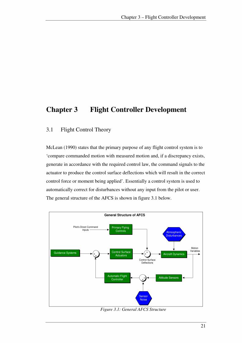
McLean (1990) states that the primary purpose of any flight control system is to
‘compare commanded motion with measured motion and, if a discrepancy exists,
generate in accordance with the required control law, the command signals to the
actuator to produce the control surface deflections which will result in the correct
control force or moment being applied’. Essentially a control system is used to
automatically correct for disturbances without any input from the pilot or user.
The general structure of the AFCS is shown in figure 3.1 below.
++
++
Motion Variables
++
Pilot's Direct CommandInputs
Control SurfaceDeflections
General Structure of AFCS
Guidance Systems
Primary Flying
Controls
Control Surface
Actuators
Attitude Sensors
Aircraft Dynamics
Automatic FlightController
Sensor
Noise
Atmospheric
Disturbances
Figure 3.1: General AFCS Structure
Chapter 3 – Flight Controller Development
22
The design of the AFCS will form the bulk of the content for this project. The
ability to achieve straight, level flight is crucial for success. There are many
various methods of designing automatic flight controllers and this project aims at
implementing probably the simplest form of these. A simple error correction
controller should be sufficient to achieve stable flight and basic waypoint
navigation.
The AFCS theory for this project is ultimately based upon the equations shown
in chapter two, essentially with separate control for both longitudinal and lateral
control. These equations, based on the flight dynamics of the aircraft, will
provide a reasonable starting point from which to predict the behaviour of the
system. It should be noted at this point that the AFCS for a UAV of this scale (a
small, inherently stable model aircraft travelling at relatively low speed) can
essentially be designed in two ways. The dynamics investigated in chapter two
are critical for stability in large scale aircraft, however in the case of this project;
this analysis is simply used to give a representation of the system dynamics
without the need for actual stability testing of the aircraft. The mathematical
control theory itself can be built upon to design a more conventional control
system that would no doubt be adequate for this project. However due to the
small scale of the system in question and the fact that stability data relating to a
model aircraft was difficult to obtain, a more intuitive approach was taken in
regards to controlling the stability of the aircraft. Figure 3.2 shows how the
control of the aircraft will be achieved, and where the mathematical system
dynamics analysis conducted in chapter two will feature, particularly in the
simulation stages of development.

Chapter 3 – Flight Controller Development
23
PRIMARYCONTROL
ALGORITHM(HC12)
Accelerometer
(Pitch/Roll Measurement)
Control Surface Actuators
(Servo Motor Control)"Desired" Pitch and Roll
"Actual" Pitch and Roll System Dynamics
Elevator and Rudder Deflection
Heading
Information
Figure 3.2: Primary closed loop system
An intuitive approach to stability control (essentially pitch and roll control) will
simply need to record attitude measurements, examine heading information, and
apply constraints to desired attitudes based upon the required heading. This
essentially means that if the aircraft is flying at the desired heading, then pitch
and roll simply need to be maintained at zero level (stable, level flight). If
however there is a heading error, pitch and roll constraints must be relaxed to
allow the required heading correction to take place. The system dynamics
analysed in chapter two will be important in developing timing requirements and
constraints in the primary control algorithm. The need to simulate how the
aircraft will respond to various control inputs is necessary to ensure that the
primary control algorithm does not deliver system commands that dramatically
alter the aircraft attitudes and force instability.
3.2 State Space Representation
Both the longitudinal and lateral systems described by the equations in chapter 2
can be represented in the following state space form for control system design
and simulation purposes. Not that these systems are initially characterised in the
continuous-time domain. For any computer control application it is necessary to
operate in the discrete-time domain. This will be dealt with later.
Chapter 3 – Flight Controller Development
24
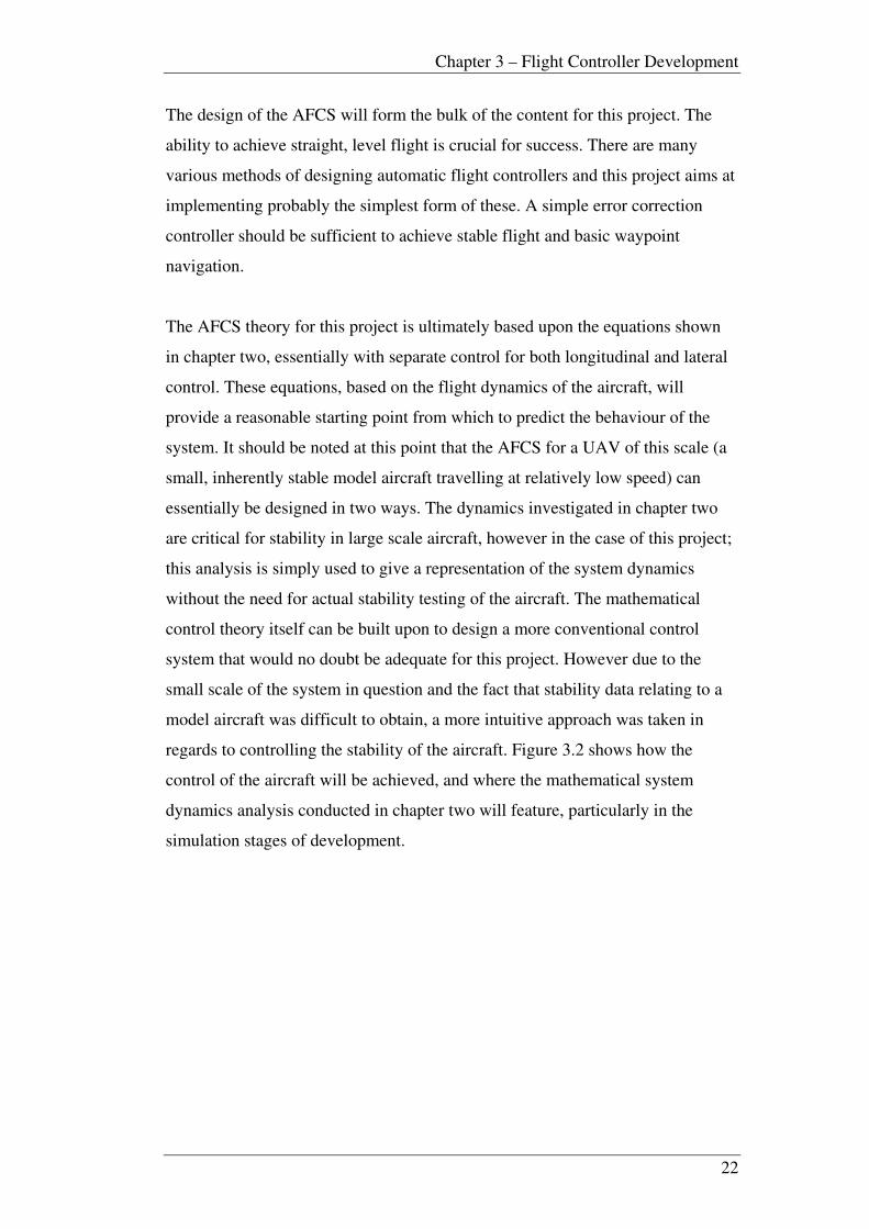
Figure 3.3: Continuous-time State Space Block Diagram Representation
Mathematically the block diagram in figure 3.3 can be represented as the
following state space equations shown in equation 3.1.
matrix forward-feed therepresents D''
matrix output therepresents C''
matrix driving therepresents B''
matrixt coefficien state therepresents A''
vectorcontrolor input therepresents u''
vectorstate therepresents x'' :Where
)()()(
)()()(
tDutCxty
tButAxtx
+=
+=•
Equation 3.1: General Form of State Equations
3.2.1 Longitudinal System
The longitudinal equations shown in equation 2.13 in the previous chapter can be
represented in state space matrix form as shown in equation 3.2.

Chapter 3 – Flight Controller Development
25
[ ]
[ ] [ ] [ ]E
EE
E
E
qwu
wu
wu
h
Q
W
U
y
M
Z
X
h
Q
W
U
U
MMMM
gUZZ
gXX
h
Q
W
U
δ
δ
γ
γ
δ
δ
δ
θ
∆+
∆
∆Θ
∆
∆
∆
=
∆
+
∆
∆Θ
∆
∆
∆
−
−
−
=
∆
Θ∆
∆
∆
∆
•
•
•
•
•
010000
0
0
0010
00100
0
0sin
0cos0
0
00
0
Equation 3.2: Longitudinal State Space Representation
The ‘C’ matrix is essentially the required parameters that are of value from a
longitudinal control perspective. In a simulation situation this matrix can be
altered to examine the effect of changes on different parameters, for example the
height of the aircraft and the pitch angle of the aircraft. The ‘C’ matrix presented
in equation 3.2 is focussed on examining the response of the height of the aircraft.
The constants shown in the ‘A’ and ‘B’ matrix are the stability derivatives
specific to the aircraft being modelled. It is at this point that adequate estimations
need to be made as stability data for the exact aircraft chosen for this project is
unavailable. This data essentially needs to be obtained through testing of the
aircraft in a wind tunnel. Wind tunnel tests are often carried out as a simulation
technique, to examine the effect of both atmospheric and control surface
disturbances on the physical dynamics of the aircraft. The stability derivatives
shown in equation 3.3 have been taken from an undergraduate project conducted
at the Queensland University of Technology that modelled the longitudinal
characteristics of a similar model aircraft in a wind tunnel (Abdullah, Fookes,
Kumar-Mills, 1998). These figures should provide the necessary accuracy for the
simulation purposes of this project.

Chapter 3 – Flight Controller Development
26
[ ]
[ ]
∆
∆Θ
∆
∆
∆
=
∆
−
+
∆
∆Θ
∆
∆
∆
−
−−
−−
−−−
=
∆
Θ∆
∆
∆
∆
•
•
•
•
•
h
Q
W
U
y
h
Q
W
U
h
Q
W
U
E
10000
0
0
9686.0
1543.0
0610.0
016010
00100
001575.01384.00102.0
00166764.22232.0
081.906762.26284.0
δ
Equation 3.3: Longitudinal Representation with Stability Derivatives
3.2.2 Lateral System
The lateral system can be represented similarly to the longitudinal system
described above. The primary difference in the lateral plane is the existence of
two control inputs. Longitudinally it is only necessary to consider the control of
the elevators, whereas in a lateral sense it is necessary to consider both rudder
and aileron control. Despite the fact that the aircraft chosen for this project does
not require aileron control, it is still important to consider this aspect during the
simulation phase, that way if the aircraft was changed at some point in the future,
simulation results would not be significantly affected. The lateral state space
description is shown in equation 3.4.

Chapter 3 – Flight Controller Development
27
[ ]
∆
∆+
∆Ψ
∆Φ
∆
∆
∆
=
∆
∆
+
∆Ψ
∆Φ
∆
∆
∆
−−
=
Ψ∆
Φ∆
∆
∆
∆
•
•
•
•
•
R
A
R
A
RA
RA
R
rpv
rpv
v
R
P
V
y
NN
LL
Y
R
P
V
NNN
LLL
U
gY
R
P
V
δ
δ
δ
δ
γ
γ
γ
δδ
δδ
δ
0010000
01000
00
00
0
00sec00
00tan10
00
00
0cos10
0
0
0
0
Equation 3.4: Lateral State Space Representation
Again the focus of the ‘C’ matrix can be altered to focus on different aspects of
the aircraft. At present (as shown in equation 3.4) the focus is placed on the roll
and yaw angles. The lateral stability derivatives shown in equation 3.5 are again
simply an estimate of the actual derivatives that could be expected from the
aircraft chosen for this project. The figures displayed are stability derivative
estimates from a twin-piston engined general aviation aircraft (McLean, 1990).
Whilst these figures will not be entirely accurate, they will be a suitable
estimation for the purposes of this analysis. Substitution of these constants is
shown in equation 3.5.
[ ]
∆
∆+
∆Ψ
∆Φ
∆
∆
∆
=
∆
∆
−−+
∆Ψ
∆Φ
∆
∆
∆
−−
−−
−−−
=
Ψ∆
Φ∆
∆
∆
∆
•
•
•
•
•
R
A
R
A
R
P
V
y
R
P
V
R
P
V
δ
δ
δ
δ
0010000
01000
00
00
1.206.0
02.162.2
05.00
00100
00010
0033.027.071.3
0036.043.271.3
061.01017.0
Equation 3.5: Lateral Representation with Stability Derivatives
Chapter 3 – Flight Controller Development
28
3.3 Transfer Function Representation
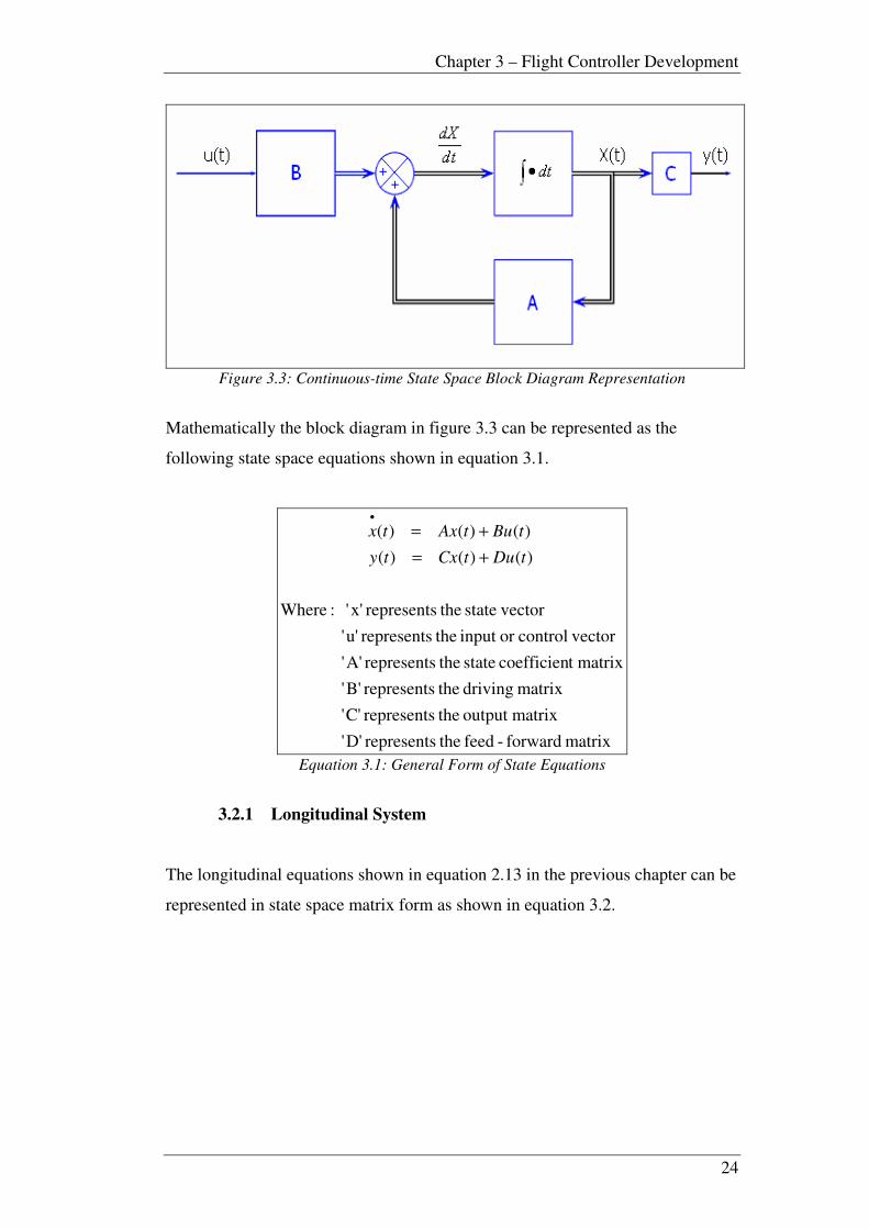
Nise (2000) states that a transfer function is a ‘viable definition for a function
that algebraically relates a system’s output to its input’. In simple block diagram
form any system can be represented as shown in figure 3.4.
Figure 3.4: Block Diagram of a Transfer Function (Nise, 2000)
The transfer function of the system is defined as shown in equation 3.6.
0
1
1
0
1
1
...
...)(
)(
)(
asasa
bsbsbsG
sR
sCn
n
n
n
m
m
m
m
+++
+++==
−−
−−
Equation 3.6: Transfer Function General Form
Note that the above representations are shown in the Laplacian ‘s’ domain, which
is directly related to the continuous-time characteristics of the system. Later the
system will be explored in the discrete-time domain or the ‘z’ domain.
3.3.1 Longitudinal Transfer Function and Stability
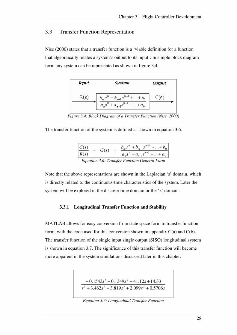
MATLAB allows for easy conversion from state space form to transfer function
form, with the code used for this conversion shown in appendix C(a) and C(b).
The transfer function of the single input single output (SISO) longitudinal system
is shown in equation 3.7. The significance of this transfer function will become
more apparent in the system simulations discussed later in this chapter.
sssss
sss
5706.0099.2819.3462.3
33.1412.411349.01543.02345
23
++++
++−−
Equation 3.7: Longitudinal Transfer Function

Chapter 3 – Flight Controller Development
29
As mentioned earlier the output of the system is really determined by the ‘C’
matrix and can be altered depending on the response in question. The transfer
function shown above is for the height of the aircraft as the output focus. If other
output variables are to be examined they would have differing, unique transfer
functions.
Closely related to the transfer function is the concept of system poles and zeros.
The poles of a transfer function are:
• The values of the Laplacian Domain (‘s’) that cause the transfer function
to become infinite.
• Any roots of the denominator that are common to the roots of the
numerator (Nise, 2000).
The zeros of a transfer function are:
• The values of the Laplacian Domain (‘s’) that cause the transfer function
to become zero.
• Any roots of the numerator that are common to the roots of the
denominator (Nise, 2000).
System poles have a significant connection with the stability of that system.
Essentially there are three rules governing the location of system poles and
consequent stability.
1) Stable systems have closed-loop transfer functions with poles only in
the left half-plane (that is with a negative real part).
2) Unstable systems have closed-loop transfer functions with at least one
pole in the right half-plane.
3) Marginally stable systems have closed-loop transfer functions with
only imaginary poles of multiplicity one, and poles in the left half-
plane (Nise, 2000).
Based on these definitions we can determine the stability of the longitudinal
system without even looking at a response. The poles of the system are
essentially the eigenvalues of the transfer function and are shown in figure 3.5.

Chapter 3 – Flight Controller Development
30
0.5054i - 0.3490-
0.5054 0.3490-
0.7515-
2.0127-
0
+
Figure 3.5: Eigenvalues (pole locations) of Longitudinal System
Applying the criteria listed above, it can be seen that the longitudinal continuous-
time system appears stable.
3.3.2 Lateral Transfer Function and Stability
Because the lateral system is not a SISO model, and actually contains two inputs
and two outputs (making the system a multi-input multi-output (MIMO) system),
there will essentially be four transfer functions, one for each combination of
input and output. These representations are shown in equation 3.8.
As above, if alternate output variables were being analysed, different transfer
functions would result.
Input: Aileron, Output: Roll Angle
07961.0897.7076.5929.2
638.9285.162.2234
2
++++
++
ssss
ss
Input: Aileron, Output: Yaw Angle
sssss
sss
07961.0897.7076.5929.2
821.51489.08662.0061.02345
23
++++
−−−−
Input: Rudder, Output: Roll Angle
07961.0897.7076.5929.2
074.44288.002.1234
2
++++
−−
ssss
ss
Input: Rudder, Output: Yaw Angle
sssss
sss
07961.0897.7076.5929.2
457.2445.0562.51.22345
23
++++
+−−−
Equation 3.8: Lateral Transfer Functions
For the pole locations of the lateral system, the four transfer functions relating
each input to each output have the same eigenvalues, and it is therefore only

Chapter 3 – Flight Controller Development
31
necessary to examine the values for any of the transfer functions. The pole
locations are as follows.
1.8430i - 0.3431-
1.8430i + 0.3431-
0.0101-
2.2326-
0
Figure 3.6: Eigenvalues (pole locations) of Lateral System
Again, after applying the stability criteria related to pole locations, the lateral
systems appear stable for each input/output combination.
3.4 Controllability and Observability
Whilst not critical to the development of the control method being implemented
in this project, the concept of system controllability and observability is essential
when designing a control system based on conventional mathematical control
techniques and utilising state variable feedback.
A control system is said to be completely controllable if it is possible to transfer
the system from any arbitrary initial state to any desired state in a finite time
period (Ogata, 1995). Controllability is important to consider as an optimal
control solution may not exist if the system is not controllable. Controllability is
determined via a controllability matrix related to the ‘A’ and ‘B’ matrices in the
continuous-time domain. Nise (2000) states the criteria for controllability as
follows:
An nth
order plant (system) whose state equation is:
BuAxx +=•
Is completely controllable if the matrix (controllability matrix),
[ ]BABAABBCn
M
12 −= L
is of rank n.

Chapter 3 – Flight Controller Development
32
Both the longitudinal and lateral systems in the AFCS are of rank 5 (essentially
the number of state variables in each system). Using MATLAB to compute the
controllability matrix (‘CM’), figure 3.7 shows the rank of this matrix and
indicates that both systems are indeed completely controllable.
Longitudinal
0 States ableUncontroll
5 States eControlabl
4875.1263253.403994.01543.00
7867.50659.21745.09686.00
3311.127867.50659.21745.09686.0
5801.1904327.931178.430982.151543.0
982.3223183.1486725.493746.0061.0
=
=
−−
−−
−−−
−−
−−−−
=MC
Lateral
0 States ableUncontroll
5 States eControlabl
8.81-8.21-8.49 2.170.580.68-2.10-0.06-00
7.0732.3-0.7515.03.41-6.38-1.022.6200
21.7-18.48.81-8.21-8.492.170.580.68-2.10-0.06-
2.3368.57.0732.3-0.7515.053.41-6.38-1.022.62
9.421.34-6.12-1.901.57-0.92-2.090.060.050
=
=
=MC
Figure 3.7: Longitudinal and Lateral Controllability
Similar to controllability, a system is said to be completely observable if every
initial state x(0) can be determined from the observation of y(t) over a finite time
period (Ogata, 1995). In a state feedback approach to control, it is a requirement
to have the feedback of all state variables. In a practical system however, some of
these state variables may not be accessible (directly measurable). It therefore
becomes necessary to estimate the value of these unknown state variables based
on the system output y(t) and an initial state x(0). If a conventional control
method was being utilised for this project a state observer system may well be

Chapter 3 – Flight Controller Development
33
required. Therefore it is useful to examine the observability of both longitudinal
and lateral systems. Nise (2000) states the criteria for observability as follows:
An nth
order plant (system) whose state and output equations are:
Cxy
BuAxx
=
+=•
Is completely observable if the matrix (controllability matrix),
[ ] |12 −= n
M CACACACO L
is of rank n.
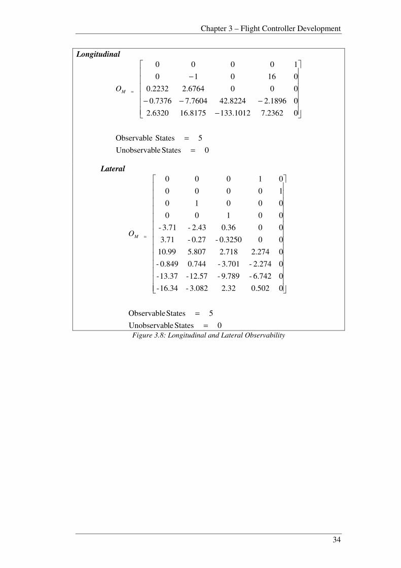
As mentioned the longitudinal and lateral systems in the AFCS are of rank 5.
Using MATLAB to compute the observability matrix (‘OM’), figure 3.8 shows
the rank of this matrix and indicates that both systems are indeed completely
observable.
Chapter 3 – Flight Controller Development
34
Longitudinal
0 States leUnobservab
5 States Observable
02362.71012.1338175.166320.2
01896.28224.427604.77376.0
0006764.22232.0
016010
10000
=
=
−
−−−
−
=MO
Lateral
0 States leUnobservab
5 States Observable
00.5022.323.082-16.34-
06.742-9.789-12.57-13.37-
02.274-3.701-0.7440.849-
02.2742.7185.80710.99
000.3250-0.27-3.71
000.362.43-3.71-
00100
00010
10000
01000
=
=
=MO
Figure 3.8: Longitudinal and Lateral Observability
Chapter 4 – Continuous-Time System Simulations
35
Chapter 4 Continuous-Time System
Simulations
4.1 Root Locus
4.1.1 Longitudinal
Root locus techniques are a powerful graphical representation of the closed loop
poles of the system as a parameter is varied (system gain etc). MATLAB allows
for easy calculation of the root locus and also gives the user the power to
examine system response parameters such as damping and percentage overshoot.
The root locus of the continuous-time longitudinal system is shown in figure 4.1.

Chapter 4 – Continuous-Time System Simulations
36
Figure 4.1: Root Locus of Longitudinal System
Figure 4.1 essentially reinforces the stability analysis conducted in section 3.3.1.
It can be seen from the figure that all poles are located in the left half-plane, thus
stabilizing the system. The root locus lines give an indication of the possible pole
locations as system gain is varied. When designing a system it is important to
restrict gain to values that will prevent the system poles from entering into the
unstable right half-plane.
MATLAB indicates that the gain value for marginal stability is approximately
0.0211. Therefore it may be necessary to scale the system down by an
appropriate gain so as to ensure closed loop stability. This will become evident
when conducting Bode Plot analysis.
4.1.2 Lateral
Realistically a root locus diagram for the lateral system does not exist, as root
locus techniques are not valid for MIMO systems. It is possible however to
simply provide a pole/zero map of the system. As mentioned earlier the pole
locations (and indeed the zero locations) of each possible input/output
combination in the lateral system are identical. A pole/zero map will not provide
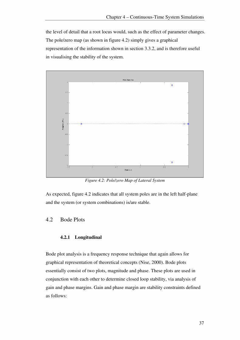
Chapter 4 – Continuous-Time System Simulations
37
the level of detail that a root locus would, such as the effect of parameter changes.
The pole/zero map (as shown in figure 4.2) simply gives a graphical
representation of the information shown in section 3.3.2, and is therefore useful
in visualising the stability of the system.
Figure 4.2: Pole/zero Map of Lateral System
As expected, figure 4.2 indicates that all system poles are in the left half-plane
and the system (or system combinations) is/are stable.
4.2 Bode Plots
4.2.1 Longitudinal
Bode plot analysis is a frequency response technique that again allows for
graphical representation of theoretical concepts (Nise, 2000). Bode plots
essentially consist of two plots, magnitude and phase. These plots are used in
conjunction with each other to determine closed loop stability, via analysis of
gain and phase margins. Gain and phase margin are stability constraints defined
as follows:

Chapter 4 – Continuous-Time System Simulations
38
• Gain margin is the change in open loop gain (in dB) required at 180o of
phase shift to make the closed-loop system unstable.
• Phase margin in the change in open-loop phase shift required at unity
gain to make the closed-loop system unstable (Nise, 2000).
As mentioned earlier, it has been established from the root locus plot that the
system is required to be scaled down by a gain value of less than 0.0211 so as to
ensure closed loop stability. MATLAB again allows for easy determination of
gain and phase margin via Bode plotting. The Bode plot of the longitudinal
system with gain and phase margin is shown in figure 4.3.
Figure 4.3: Bode Plot of Longitudinal System
Figure 4.3 indicates that the gain margin of the system is 7.81 dB and the
corresponding phase margin is 72.1o. MATLAB also indicates closed loop
system stability.

Chapter 4 – Continuous-Time System Simulations
39
4.2.2 Lateral
As with root locus analysis, Bode plots for the lateral system will not be of great
use for stability analysis. The concept of gain and phase margin is relevant only
for SISO systems and is therefore not valid for the lateral MIMO system. For
reference, the Bode plots for each lateral system combination have been shown
in figure 4.4.
Figure 4.4: Bode Plots of Lateral System
4.3 Longitudinal System Responses
4.3.1 Step Response
A unit step input is essentially a continual unity ‘hold’ on the system input.
Before any actual simulation is carried out, it is possible to predict the response
of the system (that is the aircraft itself) to this unit step. Essentially, if a step
input was applied to the elevator (as is the case in the longitudinal system) it

Chapter 4 – Continuous-Time System Simulations
40
would be expected that the aircraft would simply gain altitude at a constant rate.
This is indeed the case as figure 4.5 highlights. Note that the output matrix ‘C’ in
this case is set to observe the effect of the control input on the altitude of the
aircraft.
Figure 4.5: Step Response (‘C’ focus - Altitude) of Longitudinal System
Another important output characteristic to investigate with regards to the
longitudinal system is the pitch angle (Θ). Intuitively it can be expected that the
pitch angle reaction to a unit step input would be to simply settle on a constant
value, as a constant increase aircraft altitude (as shown in figure 4.5) will
essentially result in a constant pitch angle. This phenomenon is displayed in
figure 4.6.

Chapter 4 – Continuous-Time System Simulations
41
Figure 4.6: Step Response (‘C’ focus – Pitch Angle) of Longitudinal System
Figures 4.5 and 4.6 indicate that the longitudinal system is responding as
expected to a unit step input.
4.3.2 Impulse Response
An impulse input is another form of control input that can be applied to the
system. An impulse implies that the input control surface (in the longitudinal
case, the elevator) is subject to a ‘zero-time’ unit pulse. Whilst in practice a true
impulse input is impossible (nothing can be ‘zero-time’), it is useful to look at
the response of the system to a ‘short’ pulse of its input. Intuitively, a ‘short’
pulse on the elevator of the aircraft should result in a slight gain in altitude before
settling at the new altitude. This is confirmed by the impulse response of the
aircraft (altitude as the focus) shown in figure 4.7.
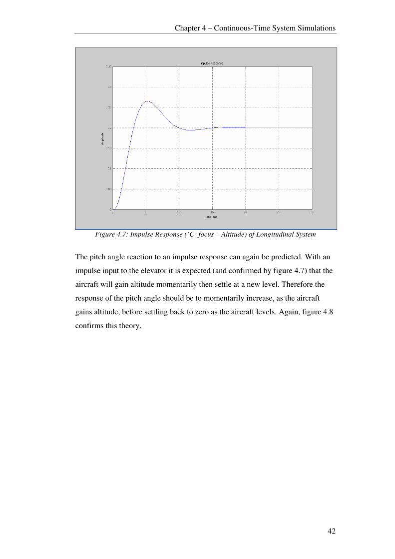
Chapter 4 – Continuous-Time System Simulations
42
Figure 4.7: Impulse Response (‘C’ focus – Altitude) of Longitudinal System
The pitch angle reaction to an impulse response can again be predicted. With an
impulse input to the elevator it is expected (and confirmed by figure 4.7) that the
aircraft will gain altitude momentarily then settle at a new level. Therefore the
response of the pitch angle should be to momentarily increase, as the aircraft
gains altitude, before settling back to zero as the aircraft levels. Again, figure 4.8
confirms this theory.

Chapter 4 – Continuous-Time System Simulations
43
Figure 4.8: Impulse Response (‘C’ focus – Pitch Angle) of Longitudinal System
Figures 4.7 and 4.8 again confirm that the longitudinal system is responding as
predicted and expected.
4.4 Lateral System Responses
4.4.1 Step Response
As previously discovered, the MIMO lateral system will have four combinations
of input/output. The primary responses that require further analysis essentially
depend on the type of aeroplane chosen as the prototyping platform. For example,
some model aircraft do not utilise aileron control at all and simply rely on the
combination of rudder deflections and wing structure to initiate a turn. For
aircraft such as these, obviously the analysis of responses to aileron input is not
necessary. Figure 4.9 shows the step responses for each of the four combinations.

Chapter 4 – Continuous-Time System Simulations
44
Figure 4.9: Step Responses of Lateral System
The primary response to focus on in figure 4.9 is the response from rudder to
yaw (essentially direction). This response is important, because the aircraft
chosen for this project does not have aileron control, and also because one of the
key design issues is the ability to correct the flight path of the aircraft to fly a
pre-determined route. Again, intuitively it can be predicted that a unit step
response on the rudder will result in a constant change in direction (yaw) similar
to the constant altitude increase with a step input to the elevator. This is indeed
reinforced by figure 4.9.
4.4.2 Impulse Response
The primary focus of the impulse response analysis is again on the response of
the yaw angle to a rudder impulse. Here it is also interesting to examine the
effect of roll angle to an impulse on the aileron. Intuitive conclusions can again
be drawn as an impulse input to the rudder of the aircraft will basically alter the
yaw angle marginally before settling at a new value. Similar conclusions can be
drawn in regards to an impulse on the aileron. Here it is expected that this form
of input would result in a momentary increase in roll angle before the aircraft

Chapter 4 – Continuous-Time System Simulations
45
once again settles at zero roll angle. These two conclusions are validated by
figure 4.10.
Figure 4.10: Impulse Responses of Lateral System
From these two simple simulations (shown in figures 4.9 and 4.10) it is evident
that the lateral system, like the longitudinal system, will respond adequately to
control inputs. The time-scale shown for the lateral system is inaccurate for the
model aircraft in question. The lateral stability derivatives for a model aircraft
could not be found, therefore as mentioned in chapter 3, derivatives from a twin-
piston engined general aviation aircraft (McLean, 1990) were used. The time
scale appears unnaturally large, as the forward velocity of the simulations was
maintained at the same value as the longitudinal system tests. The velocity of a
model aircraft would clearly not be feasible for a general aviation aircraft, hence
the exceedingly large time scale of the lateral system. For a more detailed
analysis of response times the lateral stability data for a model aircraft should be
determined (see section 8.3).
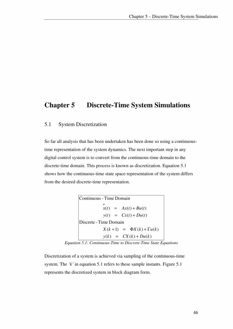
Chapter 5 – Discrete-Time System Simulations
46
Chapter 5 Discrete-Time System Simulations
5.1 System Discretization
So far all analysis that has been undertaken has been done so using a continuous-
time representation of the system dynamics. The next important step in any
digital control system is to convert from the continuous-time domain to the
discrete-time domain. This process is known as discretization. Equation 5.1
shows how the continuous-time state space representation of the system differs
from the desired discrete-time representation.
)()()(
)()()1(
Domain Time-Discrete
)()()(
)()()(
Domain Time-Continuous
kDukCXky
kukXkX
tDutCxty
tButAxtx
+=
Γ+Φ=+
+=
+=•
Equation 5.1: Continuous-Time to Discrete-Time State Equations
Discretization of a system is achieved via sampling of the continuous-time
system. The ‘k’ in equation 5.1 refers to these sample instants. Figure 5.1
represents the discretized system in block diagram form.
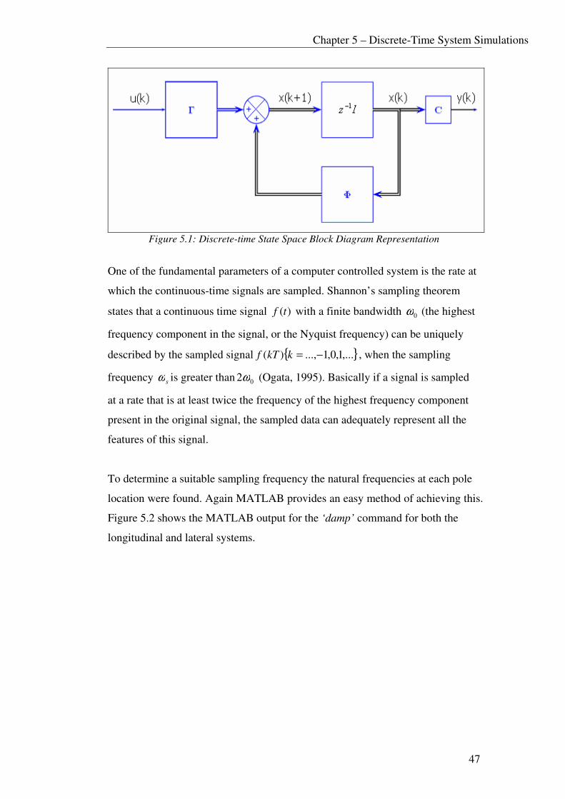
Chapter 5 – Discrete-Time System Simulations
47
Figure 5.1: Discrete-time State Space Block Diagram Representation
One of the fundamental parameters of a computer controlled system is the rate at
which the continuous-time signals are sampled. Shannon’s sampling theorem
states that a continuous time signal )(tf with a finite bandwidth 0ω (the highest
frequency component in the signal, or the Nyquist frequency) can be uniquely
described by the sampled signal { },...1,0,1...,)( −=kkTf , when the sampling
frequency sω is greater than 02ω (Ogata, 1995). Basically if a signal is sampled
at a rate that is at least twice the frequency of the highest frequency component
present in the original signal, the sampled data can adequately represent all the
features of this signal.
To determine a suitable sampling frequency the natural frequencies at each pole
location were found. Again MATLAB provides an easy method of achieving this.
Figure 5.2 shows the MATLAB output for the ‘damp’ command for both the
longitudinal and lateral systems.

Chapter 5 – Discrete-Time System Simulations
48
Figure 5.2: System Poles Damping and Natural Frequency
From figure 5.2 it can be seen that the highest frequency component in the
longitudinal system is 2.01 rad/s, and the corresponding lateral high frequency is
2.23 rad/s. Sampling theorem suggests that the sampling rate should be at least
twice the highest frequency component, therefore to be safe a factor of five times
the highest component will be used. Equation 5.2 shows how to calculate a
suitable sampling interval for each system based on this frequency data.
Longitudinal Lateral
s
wT
Hz
Hz
sradw
sradw
n
n
n
625.0
5
1
6.1
2
05.10
/05.105
/01.2
=
=∴
=
=
=
=
π
s
wT
Hz
Hz
sradw
sradw
n
n
n
564.0
5
1
77.1
2
15.11
/15.115
/23.2
=
=∴
=
=
=
=
π
Equation 5.2: Determination of Sampling Rate
Now that the sampling rate of each system has been decided upon, MATLAB
allows for simple conversion from continuous-time domain to discrete-time
domain using the ‘c2d’ command. The output of this conversion is shown for
both systems in figures 5.3 and 5.4.

Chapter 5 – Discrete-Time System Simulations
49
Longitudinal
[ ]
[ ]
∆
∆Θ
∆
∆
∆
=
+=
∆
+
∆
∆Θ
∆
∆
∆
=+
∆
∆Θ
∆
∆
∆
Γ+Φ=+
h
Q
W
U
ky
kDukCXky
h
Q
W
U
k
h
Q
W
U
kukXkX
10000)(
)()()(
0.162
0.173
0.516
1.76
1.40-
19.941.090.333-0.026
00.9950.540.016-0.002
00.02-0.660.04-0.008
00.184.130.070.03-
05.18-5.64-0.53-0.71
)1(
)()()1(
Eδ
Equation 5.3: Discrete-Time State Space Representation of Longitudinal System
Lateral
∆Ψ
∆Φ
∆
∆
∆
=
+=
∆
∆
−−
−−
−
+
∆Ψ
∆Φ
∆
∆
∆
=+
∆Ψ
∆Φ
∆
∆
∆
Γ+Φ=+
R
P
V
ky
kDukCXky
R
P
V
kR
P
V
kukXkX
R
A
10000
01000)(
)()()(
29.002.0
07.028.0
88.011.0
08.080.0
29.001.0
10.06-0.420.03-0.51
01.040.100.310.31-
00.31-0.350.10-1.57
00.190.390.270.71-
00.27-0.41-0.03-0.46
)1(
)()()1(
δ
δ
Equation 5.4: Discrete-Time State Space Representation of Lateral System
After system discretization it is necessary to again examine system responses to
ensure that the digital control system will respond as close as possible to the time
domain responses.

Chapter 5 – Discrete-Time System Simulations
50
5.2 Longitudinal System Responses
5.2.1 Step Response
When discretizing any system it should be expected that the responses should not
be altered significantly. Output amplitude variations may be expected however
this does not affect the response significantly and can easily be corrected by a
simple gain constant. Response time should be the same as in the continuous-
time domain. The step for the discretized longitudinal system (with a zero-order-
hold (ZOH) and output focussed on aircraft altitude) is shown in figure 5.5, and it
can be seen that, as expected it is in the same form of the continuous-time
response detailed in the chapter 4.
Figure 5.3: Step Response (‘C’ focus - Altitude) of Discretized Longitudinal System
Similarly, figure 5.6 details the expected step response of the dicretized system
with regards to pitch angle.

Chapter 5 – Discrete-Time System Simulations
51
Figure 5.4: Step Response (‘C’ focus – Pitch Angle) of Discretized Longitudinal System
5.2.2 Impulse Response
Figures 5.7 and 5.8 detail the impulse responses for the altitude and pitch angle
of the discretized longitudinal system respectively. Again, these are similar to the
continuos-time responses.
All of the longitudinal responses are performing as expected. This indicates that
by discretizing the system, the aircraft will continue to respond adequately (in the
longitudinal axis) to control inputs. It can also be seen from figures 5.5 to 5.8 that
timing issues (such as settling times, rise times etc) are identical to the
continuous-time simulations. Conversion is of course required from number of
samples to time, however analysis of this conversion (not shown) shows that
timing hasn’t been altered.

Chapter 5 – Discrete-Time System Simulations
52
Figure 5.5: Impulse Response (‘C’ focus - Altitude) of Discretized Longitudinal System
Figure 5.6: Impulse Response (‘C’ focus – Pitch Angle) of Discretized Longitudinal
System

Chapter 5 – Discrete-Time System Simulations
53
5.3 Lateral System Responses
5.3.1 Step Response
Again there is no expected variation between the discrete-time and continuous-
time lateral responses (excluding amplitudes as discussed earlier). The step
responses of the discretized lateral system are shown in figures 5.9 and 5.10.
These simulations have been divided to allow for expansion of the x-axis in order
to display a similar time base to that of the continuous-time simulations.
The sample points in these responses are difficult to distinguish simply because
of the number of samples required to achieve a similar time base to that of the
continuous-time simulations. These figures indicate that the step responses of the
discrete-time lateral system are adequate.
Figure 5.7: Step Response of Lateral System (Input – Rudder)
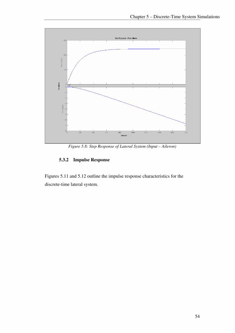
Chapter 5 – Discrete-Time System Simulations
54
Figure 5.8: Step Response of Lateral System (Input – Aileron)
5.3.2 Impulse Response
Figures 5.11 and 5.12 outline the impulse response characteristics for the
discrete-time lateral system.

Chapter 5 – Discrete-Time System Simulations
55
Figure 5.9: Impulse Response of Lateral System (Input –Rudder)
Figure 5.11 indicates some initial oscillations in the early stages of the rudder to
roll system. This is not a significant problem for this project due to the inherently
stable nature of the aircraft chosen. If a more traditional control method was
being employed, the introduction of state feedback and possibly a state observer
system would reduce these oscillations. State feedback is basically a manual pole
placement technique that allows the designer to choose pole locations for a
desired response and force the system to exhibit that response. This process will
not be outlined in this dissertation, however should a future project wish to
design a more conventional control system; all previous design and simulation
information would provide a useful starting point for the implementation of a
state feedback regulator and state observer.
Chapter 5 – Discrete-Time System Simulations
56
Figure 5.10: Impulse Response of Lateral System (Input – Aileron)
Overall, all responses in the discrete-time domain are sufficiently matched to
those in the continuos-time domain. As stated earlier, all of these simulations will
provide a good estimation of the system response and will help evaluate the
timing needs of the intuitive control method being employed for this project.
Future continuing projects may find it useful to take the analysis of chapters 2 to
5 and simply continue with designing a more conventional state feedback
controller.

Chapter 6 – Hardware Selection and Implementation
57
Chapter 6 Hardware Selection and
Implementation
6.1 Microcontroller
The microcontroller is the heart of any control application and must provide the
necessary computing power to handle complex control algorithms. For this
project the Card 12, HC12 controller module with MC912D60A microcontroller
has been selected primarily due to availability, ease of programming and
input/output features. The ‘D60A is a member of Freescale’s (formerly
Motorola’s) HC12 Microcontroller family (Elektronicladen, 2005). This module
comes equipped with a version of TwinPEEKs monitor software which allows
easy downloading and programming of Flash and EEPROM Memory without the
need for additional programming hardware (Elektronikladen, 2005). The features
of the HC12 controller module are summarised in table 6.1.

Chapter 6 – Hardware Selection and Implementation
58
Characteristic Specification
Power Supply 5 V
Typical Power Consumption 50 mA
Processor (CPU12) 16 bit
External Clock 16 MHz
System Clock 8 MHz
Flash EEPROM 60K bytes
EEPROM 1K byte
RAM 2K bytes
Asynchronous Serial Communication
(SCI)
2 channels
Serial Peripheral Interface (SPI) 1 channel
Input Capture / Output Compare Timer 8 channels
A/D Converter 16 channel / 10 Bit
Pulse Width Modulator (PWM) 4 channels Table 6.1: MC912D60A Technical Specifications (Motorola, 2000; Elektronikladen,
2005)
One of the primary features of the HC12 that will be utilised in the software
stages of this project is the Enhanced Capture Timer, utilising the input
capture/output compare channels. This basic timer consists of a 16-bit, software-
programmable counter driven by a prescaler. The timer can be used for many
purposes, such as input waveform measurement and generation of output
waveforms (Motorola, 2000). These two uses will be critical in sensor decoding
and aircraft servo motor control.
6.2 Aircraft
The aircraft initially chosen for this project was the GW/Slow Stick EPS300C
Park Flyer. This aircraft is a mass produced electric powered aircraft it has a
wingspan of 1.2m (Grand Wing Servo-Tech, 2005). It was initially considered
because it was simple inexpensive and robust. Also it is an inherently stable
aircraft which means if all control surfaces are trimmed correctly it will continue
to fly straight without continual input from the control surfaces (Byrne, 2005).
The power system has been upgraded since previous projects to a brushless
motor and controller and a 1200mah 11.1 volt lithium polymer battery (Byrne,
2005) to increase power so as to carry heavier payloads. The technical
specifications of the aircraft are summarised below in table 6.2.
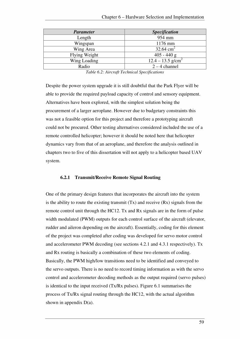
Chapter 6 – Hardware Selection and Implementation
59
Parameter Specification
Length 954 mm
Wingspan 1176 mm
Wing Area 32.64 cm2
Flying Weight 405 - 440 g
Wing Loading 12.4 – 13.5 g/cm2
Radio 2 – 4 channel Table 6.2: Aircraft Technical Specifications
Despite the power system upgrade it is still doubtful that the Park Flyer will be
able to provide the required payload capacity of control and sensory equipment.
Alternatives have been explored, with the simplest solution being the
procurement of a larger aeroplane. However due to budgetary constraints this
was not a feasible option for this project and therefore a prototyping aircraft
could not be procured. Other testing alternatives considered included the use of a
remote controlled helicopter; however it should be noted here that helicopter
dynamics vary from that of an aeroplane, and therefore the analysis outlined in
chapters two to five of this dissertation will not apply to a helicopter based UAV
system.
6.2.1 Transmit/Receive Remote Signal Routing
One of the primary design features that incorporates the aircraft into the system
is the ability to route the existing transmit (Tx) and receive (Rx) signals from the
remote control unit through the HC12. Tx and Rx signals are in the form of pulse
width modulated (PWM) outputs for each control surface of the aircraft (elevator,
rudder and aileron depending on the aircraft). Essentially, coding for this element
of the project was completed after coding was developed for servo motor control
and accelerometer PWM decoding (see sections 4.2.1 and 4.3.1 respectively). Tx
and Rx routing is basically a combination of these two elements of coding.
Basically, the PWM high/low transitions need to be identified and conveyed to
the servo outputs. There is no need to record timing information as with the servo
control and accelerometer decoding methods as the output required (servo pulses)
is identical to the input received (Tx/Rx pulses). Figure 6.1 summarises the
process of Tx/Rx signal routing through the HC12, with the actual algorithm
shown in appendix D(a).
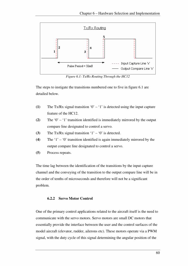
Chapter 6 – Hardware Selection and Implementation
60
Figure 6.1: Tx/Rx Routing Through the HC12
The steps to instigate the transitions numbered one to five in figure 6.1 are
detailed below.
(1) The Tx/Rx signal transition ‘0’ – ‘1’ is detected using the input capture
feature of the HC12.
(2) The ‘0’ – ‘1’ transition identified is immediately mirrored by the output
compare line designated to control a servo.
(3) The Tx/Rx signal transition ‘1’ – ‘0’ is detected.
(4) The ‘1’ – ‘0’ transition identified is again immediately mirrored by the
output compare line designated to control a servo.
(5) Process repeats.
The time lag between the identification of the transitions by the input capture
channel and the conveying of the transition to the output compare line will be in
the order of tenths of microseconds and therefore will not be a significant
problem.
6.2.2 Servo Motor Control
One of the primary control applications related to the aircraft itself is the need to
communicate with the servo motors. Servo motors are small DC motors that
essentially provide the interface between the user and the control surfaces of the
model aircraft (elevator, rudder, ailerons etc). These motors operate via a PWM
signal, with the duty cycle of this signal determining the angular position of the
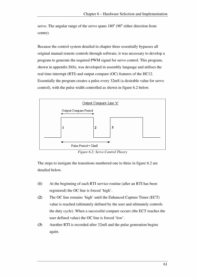
Chapter 6 – Hardware Selection and Implementation
61
servo. The angular range of the servo spans 180o (90
o either direction from
centre).
Because the control system detailed in chapter three essentially bypasses all
original manual remote controls through software, it was necessary to develop a
program to generate the required PWM signal for servo control. This program,
shown in appendix D(b), was developed in assembly language and utilises the
real time interrupt (RTI) and output compare (OC) features of the HC12.
Essentially the program creates a pulse every 32mS (a desirable value for servo
control), with the pulse width controlled as shown in figure 6.2 below.
Figure 6.2: Servo Control Theory
The steps to instigate the transitions numbered one to three in figure 6.2 are
detailed below.
(1) At the beginning of each RTI service routine (after an RTI has been
registered) the OC line is forced ‘high’.
(2) The OC line remains ‘high’ until the Enhanced Capture Timer (ECT)
value is reached (ultimately defined by the user and ultimately controls
the duty cycle). When a successful compare occurs (the ECT reaches the
user defined value) the OC line is forced ‘low’.
(3) Another RTI is recorded after 32mS and the pulse generation begins
again.
Chapter 6 – Hardware Selection and Implementation
62
For the servo to be centred (essentially 0o rotation), a pulse width of
approximately 1.5mS was needed. Figure 6.3 summarises the finer details
regarding pulse width and level of angular control.
Figure 6.3: Servo Limitations
From practical testing by inputting an arbitrary pulse time delay, it was found
that for a servo movement of 1o, a pulse width variation of approximately 9.55
µS was required. Using this information it becomes possible to completely
control the servo motor, within its 180o range, to an accuracy of approximately 1
o.
6.3 Sensors
Attitude sensors are arguably the most important part of any motion control
system, whether it be terrestrial, aquatic or air based. Without such sensors
autonomy would be impossible. The primary function of any sensor is to provide
information relating to the attitude of the object (in this case the aircraft). In a
flight control system these attitudes can include pitch, roll, yaw, velocity, altitude
and position in space. Table 6.3 provides a summary of the sensors that will be
incorporated in this project and their function (note that the compass module and
the GPS system are beyond the scope of this project and are discussed in
“Navigation and User Interface” (Knox, 2005).

Chapter 6 – Hardware Selection and Implementation
63
Sensor Type Function Specifications
Analog
Devices
ADXL213
2-axis Accelerometer Provides 2-axis tilt
sensing for pitch
and roll
Static acceleration
measurement range
of ± 1.2g
Vector 2x
Electronic
Compass
Module
Compass Module Provides heading
information • Accuracy = 2
o
• Low power
• 3-wire serial
output format
(SPI)
Garmin
GPS 35LP
Global Positioning
Unit
Provides position,
altitude and
velocity
information
• Compact Design
• Low power
• RS-232 Serial
connectivity Table 6.3: Sensor Information Summary
6.3.1 Accelerometer
The accelerometer unit is fundamental to the control of the aircraft as it provides
information relating to roll and/or pitch and/or yaw attitudes (with the number of
measurement axes depending on whether the unit is capable of dual or tri axis
measurement). The ADXL213 accelerometer that has been chosen for this
project is a simple dual axis sensor and is therefore restricted to two axes of
measurement (in this case pitch and roll attitudes). This unit has been chosen
essentially due to cost and availability. The determination of yaw information is
carried out using an electronic compass module (Knox, 2005).
The operation of the ADXL213 accelerometer module relies on a micro
machined polysilicon structure suspended with polysilicon springs over a silicon
wafer. Deformations in the polysilicon structure modulate a pulse width
modulation (PWM) oscillator which produces either a duty cycle axis output or
analogue outputs from filtered demodulation channels. The deformation of the
structure may come from a physical acceleration of the IC, or from gravity when
angularly displaced from a horizontal position (MacQueen, 2002).
For this project it was decided that the duty cycle output of the accelerometer
would be most useful and most accurate. To decode these signals using the HC12,
the input capture feature of the microcontroller was utilised. Input capture
operates by essentially capturing the value of a 16 bit free running timer module
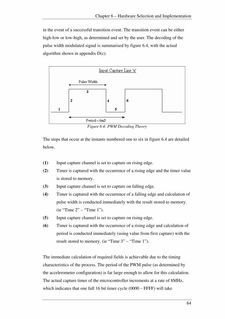
Chapter 6 – Hardware Selection and Implementation
64
in the event of a successful transition event. The transition event can be either
high-low or low-high, as determined and set by the user. The decoding of the
pulse width modulated signal is summarised by figure 6.4, with the actual
algorithm shown in appendix D(c).
Figure 6.4: PWM Decoding Theory
The steps that occur at the instants numbered one to six in figure 6.4 are detailed
below.
(1) Input capture channel is set to capture on rising edge.
(2) Timer is captured with the occurrence of a rising edge and the timer value
is stored to memory.
(3) Input capture channel is set to capture on falling edge.
(4) Timer is captured with the occurrence of a falling edge and calculation of
pulse width is conducted immediately with the result stored to memory.
(ie “Time 2” – “Time 1”).
(5) Input capture channel is set to capture on rising edge.
(6) Timer is captured with the occurrence of a rising edge and calculation of
period is conducted immediately (using value from first capture) with the
result stored to memory. (ie “Time 3” – “Time 1”).
The immediate calculation of required fields is achievable due to the timing
characteristics of the process. The period of the PWM pulse (as determined by
the accelerometer configuration) is far large enough to allow for this calculation.
The actual capture timer of the microcontroller increments at a rate of 8MHz,
which indicates that one full 16 bit timer cycle (0000 – FFFF) will take

Chapter 6 – Hardware Selection and Implementation
65
approximately 8.19 ms. It was a concern that rollovers from FFFF – 0000 by the
main timer counter would affect the calculations, however the HC12 accesses
each timer value as a single 16 bit word, hence signs are not an issue.
The decoding of the accelerometer signals results in an error value that is
proportional to the amount by which the aircraft’s pitch and roll are away from
zero (where zero error indicates level flight). These figures (one each for pitch
and roll) will be used as comparison values to an ideal state, where the ideal state
depends on whether or not the aircraft is required to be turning or simply flying
straight and level. To determine these allowable constraints, it is necessary to
analyse the output data from the accelerometer decoding to determine maximum
and minimum error values. Obviously it is not desirable to allow the aircraft a
full 180o of roll or pitch freedom about its level flight condition; therefore
constraints need to be decided upon. Figure 6.5 summarises the results of this
constraint analysis for both axes. Note that whilst pitch and roll are measured on
separate accelerometer channels, the results are identical as the measurement
range is identical in each axial plane ( g2.1± ).
Figure 6.5: Accelerometer Pitch and Roll Error Measurement Characteristics
When tested to obtain the above readings, the accelerometer was mounted on
slight angles to ensure that an error of zero was recorded for 0o roll (and pitch). It

Chapter 6 – Hardware Selection and Implementation
66
will also become necessary to mount the accelerometer in this manner when
installing the sensor into any prototyping aircraft to ensure that level flight is
indeed acknowledged by the control system as being “level flight”. From figure
6.5 it appears that the mounting angle does not tend to affect the error value over
small angular ranges (ie within the desired roll/pitch constraints). A discrepancy
does appear however for larger angular values as denoted by the maximum
achievable roll of 90o. This calibration issue could possibly be due to an internal
IC calibration error, a PCB mounting error, or perhaps even a software rounding
error (more likely a combination of the three). This problem should not be
significant as it appears that up to the designated roll constraints of
approximately 20o, the errors in either direction appear identical. Hopefully in
the process of constraining the roll and pitch of the aircraft, large angular errors
will not be experienced and therefore the problem will be minimised.
6.4 Manual Handover/System Monitoring
System monitoring is a built in device aimed at allowing automatic handover
from pilot to controller and vice versa. System monitoring will also include
circuitry to monitor the status of the HC12 to ensure that the controller is
functioning. If the controller were to fail in any way, the system monitoring
circuit would automatically revert to manual pilot control. This is an important
added safety feature and is not in essence critical to the project.
Manual/autonomous transition and autonomous/manual transition is however an
important feature that must be incorporated into any prototype.
As a prototype will not be developed for this project, a manual handover circuit
will not be constructed; however a proposed layout and design will be included
for future reference. Figure 6.6 shows a general block diagram of the proposed
manual handover/system monitoring hardware.
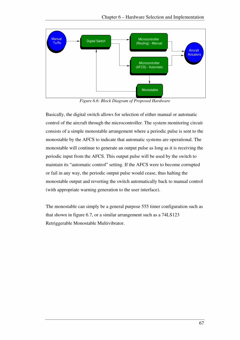
Chapter 6 – Hardware Selection and Implementation
67
Digital SwitchMicrocontroller
(Routing) - Manual
Microcontroller
(AFCS) - Automatic
Aircraft
Actuators
Monostable
Manual
Tx/Rx
Figure 6.6: Block Diagram of Proposed Hardware
Basically, the digital switch allows for selection of either manual or automatic
control of the aircraft through the microcontroller. The system monitoring circuit
consists of a simple monostable arrangement where a periodic pulse is sent to the
monostable by the AFCS to indicate that automatic systems are operational. The
monostable will continue to generate an output pulse as long as it is receiving the
periodic input from the AFCS. This output pulse will be used by the switch to
maintain its “automatic control” setting. If the AFCS were to become corrupted
or fail in any way, the periodic output pulse would cease, thus halting the
monostable output and reverting the switch automatically back to manual control
(with appropriate warning generation to the user interface).
The monostable can simply be a general purpose 555 timer configuration such as
that shown in figure 6.7, or a similar arrangement such as a 74LS123
Retriggerable Monostable Multivibrator.
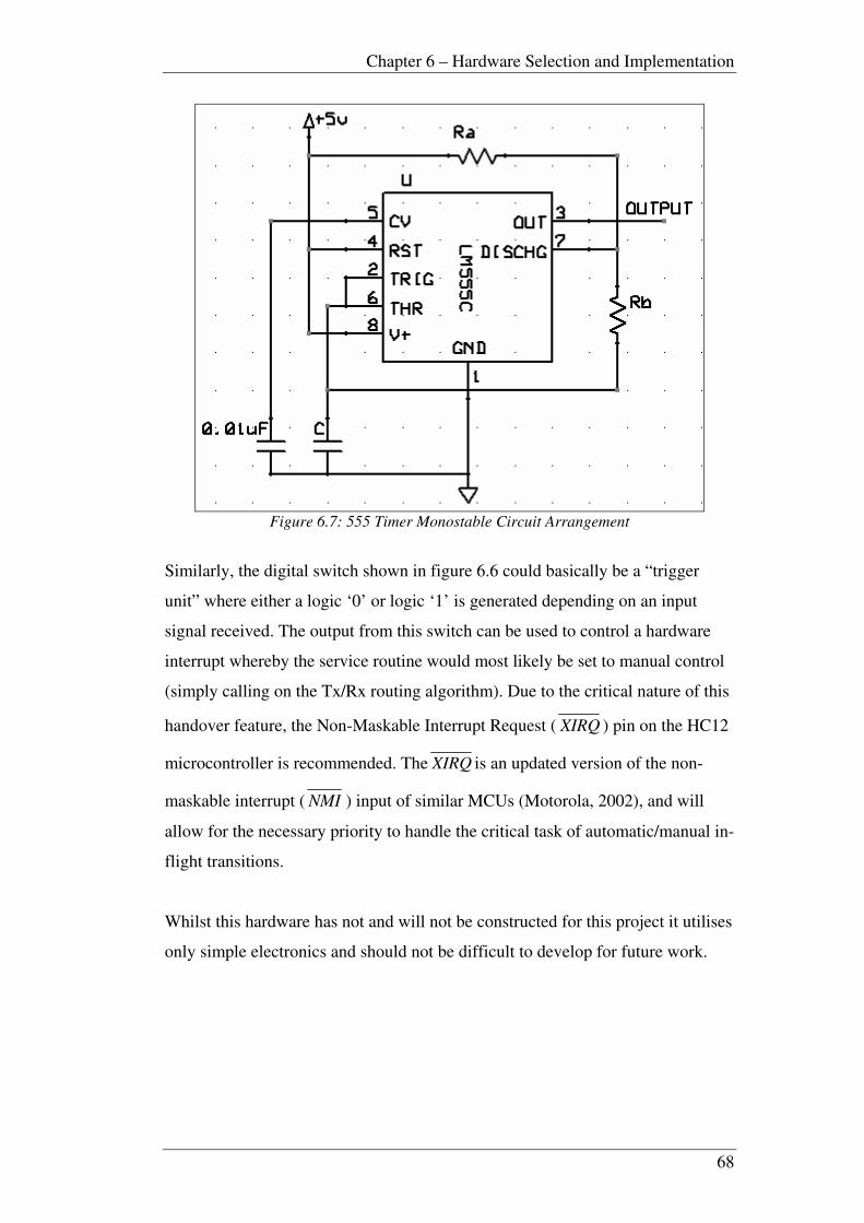
Chapter 6 – Hardware Selection and Implementation
68
Figure 6.7: 555 Timer Monostable Circuit Arrangement
Similarly, the digital switch shown in figure 6.6 could basically be a “trigger
unit” where either a logic ‘0’ or logic ‘1’ is generated depending on an input
signal received. The output from this switch can be used to control a hardware
interrupt whereby the service routine would most likely be set to manual control
(simply calling on the Tx/Rx routing algorithm). Due to the critical nature of this
handover feature, the Non-Maskable Interrupt Request ( XIRQ ) pin on the HC12
microcontroller is recommended. The XIRQ is an updated version of the non-
maskable interrupt ( NMI ) input of similar MCUs (Motorola, 2002), and will
allow for the necessary priority to handle the critical task of automatic/manual in-
flight transitions.
Whilst this hardware has not and will not be constructed for this project it utilises
only simple electronics and should not be difficult to develop for future work.

Chapter 7 – Intuitive Control and Pre-Flight Testing
69
Chapter 7 Intuitive Control and Pre-Flight
Testing
7.1 Intuitive Control versus Conventional Control
As touched upon in chapter three, an intuitive “observe-and-correct” control
system will be implemented based on simple inner loop and outer loop control
principles. This method was chosen primarily due to the simplicity of the model
aircraft system, but more importantly the lack of available data relating to the
stability analysis of a model aircraft. Some limited model aircraft stability
derivatives were available for the longitudinal system, however no similar
derivatives could be found for the lateral system. If this data could be discovered
or derived (through wind tunnel testing of a model aircraft) it is recommended
that a more conventional approach be taken towards the design of the AFCS. All
system plant data is available in chapters two and three of this dissertation, and
will not vary significantly between aeroplane types. With more accurate stability
derivatives, PID control techniques or a suitable alternative are recommended.
7.2 The Intuitive Approach
Figure 7.1 shows a block diagram representation of the control method being
employed as the AFCS for this project.

Chapter 7 – Intuitive Control and Pre-Flight Testing
70
PRIMARYCONTROL
ALGORITHM(HC12)
Accelerometer
(Pitch/Roll Measurement)
Control Surface Actuators
(Servo Motor Control)"Desired" Pitch and Roll
"Actual" Pitch and Roll System Dynamics
Elevator and Rudder Deflection
Heading
Information
Figure 7.1: Primary closed loop system
Outer loop information (or heading and navigation information) will essentially
be passed straight through to the control surface actuator controlling the heading
of the aircraft (rudder servo motor). The outer loop’s main function is to retrieve
heading updates approximately four times per second, and provide the necessary
control signal to the rudder to attempt to minimise the heading error. In between
these updates, it is the inner loop’s task to monitor and maintain the desired pitch
and roll based on allocated allowable constraints.
Figure 7.2 shows a process flow diagram detailing the functional aspects of the
primary control algorithm.

Chapter 7 – Intuitive Control and Pre-Flight Testing
71
Start
Allocate Roll Constraints
Retrieve Heading Error
Displace Rudder to MinimiseHeading Error
Sense Pitch/Roll
Characteristics
Correct ifNecessary
INNER LOOP
OUTER LOOP
Figure 7.2: Process Flow of Primary Control Algorithm
The heading information is in the form of a scaled integer so as to provide a
scaled timing value fed directly to the rudder servo control algorithm. The raw
heading information is essentially in the form of ± 180o. This raw information is
scaled according to equation 7.1.
centre) of side(either rangeangular Maximum 180
)(15 deflectionrudder allowable Maximum 1146
servo centredfor timecompareOutput 12000 :Where
*180
114612000
o
→
→
→
+= errorrawHeadingScaled
Equation 7.1: Heading Scaling
Table 7.1 indicates a range of rudder deflections expected from various raw
heading errors. Note that the information in table 7.1 was calculated using
equation 7.1.
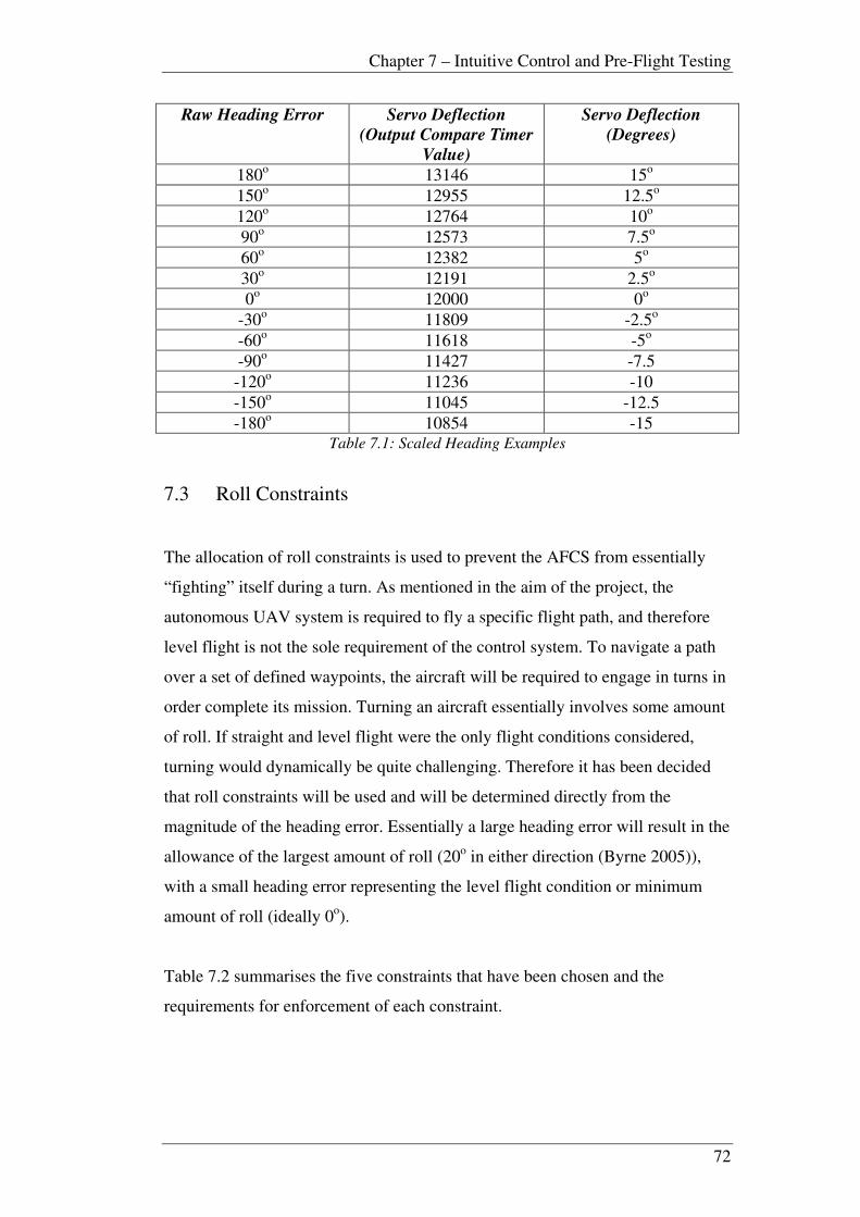
Chapter 7 – Intuitive Control and Pre-Flight Testing
72
Raw Heading Error Servo Deflection
(Output Compare Timer
Value)
Servo Deflection
(Degrees)
180o
13146 15o
150o 12955 12.5
o
120o 12764 10
o
90o 12573 7.5
o
60o 12382 5
o
30o 12191 2.5
o
0o 12000 0
o
-30o 11809 -2.5
o
-60o 11618 -5
o
-90o 11427 -7.5
-120o 11236 -10
-150o 11045 -12.5
-180o 10854 -15
Table 7.1: Scaled Heading Examples
7.3 Roll Constraints
The allocation of roll constraints is used to prevent the AFCS from essentially
“fighting” itself during a turn. As mentioned in the aim of the project, the
autonomous UAV system is required to fly a specific flight path, and therefore
level flight is not the sole requirement of the control system. To navigate a path
over a set of defined waypoints, the aircraft will be required to engage in turns in
order complete its mission. Turning an aircraft essentially involves some amount
of roll. If straight and level flight were the only flight conditions considered,
turning would dynamically be quite challenging. Therefore it has been decided
that roll constraints will be used and will be determined directly from the
magnitude of the heading error. Essentially a large heading error will result in the
allowance of the largest amount of roll (20o in either direction (Byrne 2005)),
with a small heading error representing the level flight condition or minimum
amount of roll (ideally 0o).
Table 7.2 summarises the five constraints that have been chosen and the
requirements for enforcement of each constraint.

Chapter 7 – Intuitive Control and Pre-Flight Testing
73
Heading
Error
Servo Rotation
Induced
(Degrees)
Output Compare
Timer Count (for
Servo Rotation)
Maximum
Allowable Roll
Angle (Roll
Constraints)
0o - 10
o 0
o – 0.83
o 12000 (centred) –
12000 ± 64.67
0o
10o - 30
o 0.83
o – 2.5
o 12000 ± 64.67 –
12000 ± 194
5o
30o - 80
o 2.5
o – 6.77
o 12000 ± 194 –
12000 ± 517.3
10o
80o - 120
o 6.77
o – 10.16
o 12000 ± 517.3 –
12000 ± 776
15o
120o - 180
o 10.16
o – 15.23
o 12000 ± 776 –
12000 ± 1164
20o
Table 7.2: Roll Constraint Guide
Table 7.2 was developed by basically adapting the five roll constraints to
correspond to servo rotation angular limits. In the event that a roll constraint is
exceeded, the system will correct by simply reducing the angle of deflection
applied to the rudder.
The information shown in table 7.3 was also used within the inner loop function
to compare the “actual” tilt errors to the designated constraints. This table shows
the expected error for each constraint limit.
Constraint Limit Error
20o
6
15o 4
10o 3
5o 1
0o 0
Table 7.3: Expected Errors for Constraint Limits
7.4 Primary Control Algorithm Testing
Because an aircraft was unavailable for testing purposes, an alternate method was
required to verify the functionality of the control algorithm. Obviously, the ideal
case would be to physically implement the entire system into a prototype UAV,
where the system is subject to atmospheric disturbances and dynamics of flight.
In this ideal case, issues such as the magnitudes of servo rotation, as well as the

Chapter 7 – Intuitive Control and Pre-Flight Testing
74
magnitudes of the allowable roll constraints could be tested and “fine-tuning” of
the algorithm could be conducted. However, this will be recommended as future
work, and for the testing stage of this project, the algorithm will simply be tested
without subjecting the system to the dynamics of aircraft flight.
As mentioned earlier, the system is required to control both the pitch and roll of
the aircraft. Essentially, the pitch can simply be a “set” level, whereby the
aircraft attempts to fly at the same altitude throughout its entire mission. The roll
however, as previously stated, essentially results from changes in yaw angle
required by the aircraft to complete its mission. This yaw angle, and hence the
level of roll required, will be continually changing depending on the current path
of the aircraft and its proximity in relation to the waypoint path selected. From
this information it can be concluded that the roll axis is essentially the most
important axis to consider, and therefore for testing purposes this axis will be the
focus. It should be noted here that, the algorithm derived for control of the roll
axis (shown in appendix D(d)) can be easily adapted to pitch axis control.
7.4.1 Hardware Setup
The control algorithm, shown in appendix D(d) was developed in assembly
language, and is essentially a combination of the applications listed in chapter six,
namely accelerometer decoding and servo motor control. The testing was carried
out using the accelerometer module and a single servo motor. For angular
measurements, a jig (constructed by Terry Byrne from the Faculty of
Engineering and Surveying) was used to mount the accelerometer in conjunction
with a protractor so that accurate angles of tilt could be measured. The jig used
for this testing is shown in figure 7.3.

Chapter 7 – Intuitive Control and Pre-Flight Testing
75
AccelerometerModule
Protractor
Figure 7.3: Accelerometer Testing Setup
This jig allowed for angular measurements up to ± 180o. When operated in
tandem with the accelerometer decoding program shown in appendix D(c), error
values for varying tilt angles could be identified.
For servo motor angular rotation testing, a similar setup was used. The servo
motor was placed within another jig with a 360o protractor for angular
measurement placed above. This particular setup is shown in figure 7.4.
Servo Motor
Protractor
Figure 7.4: Servo Motor Testing Setup
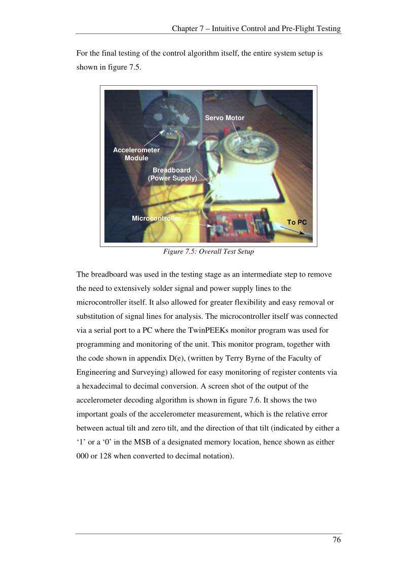
Chapter 7 – Intuitive Control and Pre-Flight Testing
76
For the final testing of the control algorithm itself, the entire system setup is
shown in figure 7.5.
AccelerometerModule
Servo Motor
Microcontroller
Breadboard (Power Supply)
To PC
Figure 7.5: Overall Test Setup
The breadboard was used in the testing stage as an intermediate step to remove
the need to extensively solder signal and power supply lines to the
microcontroller itself. It also allowed for greater flexibility and easy removal or
substitution of signal lines for analysis. The microcontroller itself was connected
via a serial port to a PC where the TwinPEEKs monitor program was used for
programming and monitoring of the unit. This monitor program, together with
the code shown in appendix D(e), (written by Terry Byrne of the Faculty of
Engineering and Surveying) allowed for easy monitoring of register contents via
a hexadecimal to decimal conversion. A screen shot of the output of the
accelerometer decoding algorithm is shown in figure 7.6. It shows the two
important goals of the accelerometer measurement, which is the relative error
between actual tilt and zero tilt, and the direction of that tilt (indicated by either a
‘1’ or a ‘0’ in the MSB of a designated memory location, hence shown as either
000 or 128 when converted to decimal notation).

Chapter 7 – Intuitive Control and Pre-Flight Testing
77
Figure 7.6: Screen Shot of TwinPEEKs Monitor Program
7.4.2 Software Setup
Figure 7.7 shows a software flow chart of the sub-routines that are called upon to
provide the necessary control of aircraft roll. The actual coded program is shown
in appendix D(d). Note that the outer loop control (heading information) is
simply inputted manually for testing purposes. In a realistic flight situation, this
value would be updated approximately every 0.25 seconds.
Column 1 – Relative Error
Column 2 – Direction of Tilt

Chapter 7 – Intuitive Control and Pre-Flight Testing
78
START
Setup ICOC
Allocate
Move
Constraint
PWM Decode
Calc DC
Compare
Printcheck
Causes servo deflection in attempt to minimise heading error(utilises RTI facility)
Allocates "desired" roll constraint values for each heading error
magnitude (actual constraint values are in a similar form to the error values recorded in the pwm decoding routine)
Checks heading error magnitude and selects corresponding
roll constraint
Calculates the relative error between level flight and the
measured tilt angle (ie "actual" roll)
Compares the "actual" roll to the "allowable/desired" roll, and if "actual"exceeds "allowable/desired", reduces servo deflection
Prints 'roll error', 'roll direction' and 'constraint selected' to the PCterminal screen for verification purposes
Decodes PWM signals from accelerometer using input capture
Sets up input capture/output compare channels for accelerometer
decoding and servo motor control
Outer Loop
(Not present for testing)
Inner Loop
Figure 7.7: Software Flow Chart of Primary Control Algorithm
To test this primary algorithm, a heading value was manually inserted into the
required memory location. In a prototype situation this value would be retrieved
from communications with the navigation system, at a rate of approximately four
times per second. To test all possible situations, the manual input of the heading
information was made a number of times with varying magnitudes. With this
manual input, the inner loop function will basically just monitor the roll
characteristics until process is halted, acting only when the measured roll is
outside of the selected constraint.
7.4.3 Test Results
Manually inserted values of heading were chosen carefully so as to ensure all
cases of roll constraint were tested. The tests showed that the initial heading
information produced the required angular deflection of the servo motor. From
this point the accelerometer module was manually rotated using the jig shown
above in figure 7.3. The tests concluded that for each constraint value, the servo
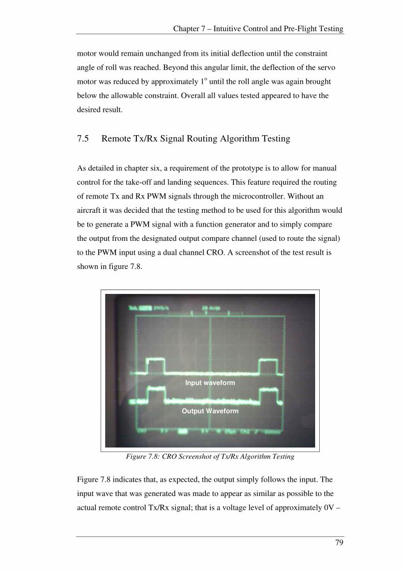
Chapter 7 – Intuitive Control and Pre-Flight Testing
79
motor would remain unchanged from its initial deflection until the constraint
angle of roll was reached. Beyond this angular limit, the deflection of the servo
motor was reduced by approximately 1o until the roll angle was again brought
below the allowable constraint. Overall all values tested appeared to have the
desired result.
7.5 Remote Tx/Rx Signal Routing Algorithm Testing
As detailed in chapter six, a requirement of the prototype is to allow for manual
control for the take-off and landing sequences. This feature required the routing
of remote Tx and Rx PWM signals through the microcontroller. Without an
aircraft it was decided that the testing method to be used for this algorithm would
be to generate a PWM signal with a function generator and to simply compare
the output from the designated output compare channel (used to route the signal)
to the PWM input using a dual channel CRO. A screenshot of the test result is
shown in figure 7.8.
Input waveform
Output Waveform
Figure 7.8: CRO Screenshot of Tx/Rx Algorithm Testing
Figure 7.8 indicates that, as expected, the output simply follows the input. The
input wave that was generated was made to appear as similar as possible to the
actual remote control Tx/Rx signal; that is a voltage level of approximately 0V –
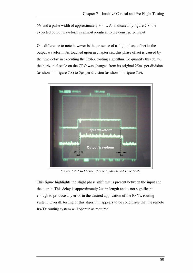
Chapter 7 – Intuitive Control and Pre-Flight Testing
80
5V and a pulse width of approximately 30ms. As indicated by figure 7.8, the
expected output waveform is almost identical to the constructed input.
One difference to note however is the presence of a slight phase offset in the
output waveform. As touched upon in chapter six, this phase offset is caused by
the time delay in executing the Tx/Rx routing algorithm. To quantify this delay,
the horizontal scale on the CRO was changed from its original 25ms per division
(as shown in figure 7.8) to 5µs per division (as shown in figure 7.9).
Output Waveform
Input waveform
2us 2us
Figure 7.9: CRO Screenshot with Shortened Time Scale
This figure highlights the slight phase shift that is present between the input and
the output. This delay is approximately 2µs in length and is not significant
enough to produce any error in the desired application of the Rx/Tx routing
system. Overall, testing of this algorithm appears to be conclusive that the remote
Rx/Tx routing system will operate as required.
Chapter 7 – Intuitive Control and Pre-Flight Testing
81
7.6 Future Testing
7.6.1 Primary Control Algorithm
The “fine-tuning” of this algorithm as mentioned above is necessary for future
progress with this control method. The figures used as limits for servo deflection
and maximum allowable roll angle are realistically just guesses based on flight
experience with manual control of a remote controlled aircraft. For example the
maximum servo motor deflection of 15o chosen as the limit for this project may
well be too large, and as such may cause the aircraft to become unstable very
quickly. Alternatively, this figure may be too small, and hence result in an
excessively large turning radius, thus making navigation difficult. Either way,
more analysis needs to be conducted into the dynamics of model aircraft flight.
This again reinforces the need for more accurate model aircraft stability data. If
this data was known, the analysis of maximum rudder (servo) deflections, as well
as maximum allowable roll angles, could be conducted via the MATLAB
simulation process detailed earlier in this dissertation. Other “fine-tuning” could
also be applied to the servo angle reduction phase of the control algorithm, once
outside of the allowable roll range. As mentioned, once the roll becomes too
excessive, the servo deflection is currently being reduced by approximately 1o.
Again, this may be too low or indeed too high for practical purposes.
7.6.2 Manual Handover and System Monitoring
Whilst this feature has not yet been constructed and can therefore not be
physically tested, it is obviously recommended that for future work the designs
outlined in section 6.4 of this dissertation should be adequately tested before any
physical implementation. This testing should ideally be conducted with the
remote controlled unit chosen for a prototype aircraft. However if this is again
unavailable, the circuit can also be tested by generating a similar ‘handover’
signal to what is expected from the remote unit itself. Whilst the algorithm for
manual control of the aircraft has been written, the primary control algorithm
needs to be added to incorporate this manual feature. As mentioned, the use of
Chapter 7 – Intuitive Control and Pre-Flight Testing
82
the XIRQ non-maskable interrupt feature of the HC12 is recommended as the
basis for the incorporation of the manual/automatic handover system. Also, for
system monitoring purposes, a periodic pulse generator needs to be incorporated
into the primary control algorithm, possibly after each inner loop measurement of
the pitch and roll characteristics of the aircraft. The periodicity of this pulse
should be such that, if a failure occurs within the primary control system,
reaction time in reverting to manual control is minimised.

Chapter 8 - Discussion
83
Chapter 8 Discussion and Conclusions
8.1 Overall System Analysis
The development of a prototype autonomous vehicle system is a significantly
complex task no matter what platform is desired (aquatic, air or terrestrial).
Extensive theoretical research, combined with software, hardware and suitable
system testing has allowed this project to give an insight into these complexities
across all fields. To analyse the achievements and progress of the autonomous
UAV system as a whole, it is necessary to revisit the aims and objectives of this
project as outlined in chapter 1.
Research has indicated that the field of autonomous robotics is a fast changing
and dynamic field of science and engineering. With technological advances
rapidly becoming commercially available, low cost UAV systems are becoming
more attractive for an ever increasing list of applications. Aside from hardware
advances themselves, control techniques used for autonomous capability are also
a fast changing, dynamic field of research within the scientific and engineering
sectors. Control techniques range from simple “observe-and-correct” type
systems, to more conventional approaches such as state feedback and PID based
control. Recent shifts have also seen the evolution adaptive control techniques
utilising almost “artificial intelligence” like systems.

Chapter 8 - Discussion
84
The control technique utilised for this project was a simple “observe-and-correct”,
heading error minimisation system. It was observed that this is not the ideal
approach to be taken in regards to control system design, primarily due to
stability concerns. By utilising this approach, the stability analysis of the AFCS
is essentially just a “guess and check” method, requiring extensive manual flight
tests of an actual model aircraft to determine various timing constraints and
system responses. The best form of control for this type of simple UAV platform
would be a conventional control system design approach, utilising state feedback,
PID control and possibly an observer system. Before a method such as this can
be developed however, more research needs to be carried out into the dynamics
of the chosen model aircraft. These physical characteristics can be directly
applied to the theory outlined in chapters 2 – 5, and it was the lack of this
physical dynamics data that restricted the use of a conventional control approach
for this project. It is hoped that much of the theory outlined in this dissertation
will provide the necessary starting point for further work.
The hardware selection for this project was governed primarily by the need to
minimise costs. The HC12 microcontroller unit that was chosen to be the heart of
the AFCS, proved to be adequate in achieving all required tasks. The ADXL213
accelerometer module gave the desired accuracy of roll and pitch measurement,
however it was noted that care must be taken in the calibration and mounting of
the unit as it appears that ‘level’ to the human eye may not necessarily be ‘level’
to the electronics of the accelerometer. Further hardware does need to be
developed for successful prototyping of a similar UAV system. Manual handover
is a critical part of the current system configuration, and a system monitoring
feature is important in meeting relevant legal and ethical requirements. Designs
have been outlined in chapter 6, and can be used as a starting point for the
development of this final hardware.
The intuitive control approach itself appears in theory to be able to provide the
necessary path navigation that it is intended. Despite this confidence in the
system, it is still largely untested in a real flight situation. With the eventual
acquirement of an aircraft, fine tuning of this AFCS algorithm could be
conducted, with the end result being a viable (but controlled) test flight. Probably

Chapter 8 - Discussion
85
more significant to this project was the testing of individual control areas within
the primary AFCS itself. Requirements such as accelerometer decoding and
interpreting, servo motor control, and remote Rx/Tx routing are critical to any
similar UAV system. These assembly language codes have been tested and do
operate as expected, and can be incorporated into any future system with
confidence.
Overall, without any actual flight testing having been conducted, the AFCS
system developed appears to be able to provide the necessary autonomy. More
importantly the lead-up stages to this design (dynamics analysis and simulation
methods) can be utilised as a starting point for a more conventional control
approach. The hardware selected for autonomy is adequate for either control
approach, and coding has been developed specifically for control and
interpretation of these hardware components.
8.2 Limitations Encountered
A summary of the limitations encountered throughout the course of this project is
important for the future development and expansion possibilities of this
autonomous UAV topic. The primary limitation that was encountered essentially
shaped the course of this project by limiting the development of a more
conventional control approach. As previously mentioned, the dynamics analysis
conducted in chapter 2 is common for all aeroplane types (with some
simplification or expansion depending on the type of plane). The eventual result
of this analysis should have been the derivation of a state space plant matrix
system describing the dynamic characteristics of the model aircraft to be used as
the platform for the UAV. This plant matrix forms the initial start point for the
design of a conventional state feedback, PID control system as shown in figure
8.1.

Chapter 8 - Discussion
86
Figure 8.1: Conventional Control Approach
As indicated by figure 8.1, the ‘plant’ is essentially a representation of the
dynamics of the system. This information relating to the dynamics of a model
aircraft (most model aircraft of a similar size would have similar dynamic
characteristics) was not readily available for use in developing the ‘plant’ system.
Data such as this is available for larger scale aircraft (as was used for the
simulations for this project), however extensive research uncovered very little
relating to model aircraft platform. The data itself is generally obtained through
wind tunnel testing of the aircraft, where control surface deflections are applied
to the aircraft and system responses are observed in a controlled environment.
Many hours of research were put into attempts to locate relevant data however
due to time constraints; the possibility of implementing a form of conventional
control was abandoned. In the end this lack of the dynamics data was the
determining factor for the adoption of the “observe-and-correct” control method.
Aside from this major limitation, the only other influential limitation encountered
was the unavailability of a testing aircraft. Due to funding constraints the
University was unable to purchase an aircraft for prototyping and testing
purposes. In terms of system testing, suitable alternatives were sought and all
aspects were tested to an adequate level without any actual physical prototyping.
For example the servo motor control algorithms were simply tested on a single
servo motor similar to which is found in any commercially available model
aircraft. The one limitation of the unavailability of the aircraft itself was in
regards to testing the primary AFCS control algorithm. As mentioned previously,
“fine tuning” of this aspect of the project could not be conducted due to the
unavailability of a suitable aircraft. It is hoped that for future project work in this

Chapter 8 - Discussion
87
field of autonomous UAV systems, that a suitable aircraft is available to
complete this final testing phase.
8.3 Recommendations for Future Work
As mentioned on several occasions, with the unavailability of an aircraft the
perceived focus of this project has shifted slightly from the actual construction of
a working prototype UAV system, to providing the building blocks and
necessary background information for a future continuing project. Obviously,
before even mentioning any future recommendations, the primary aim for any
future research work in this field would be to address the limitations that have
been detailed above. So for simplicity, recommendations have been summarised
in point form below:
1) Obtain stability and dynamics data for a model aircraft.
This data may be already accessible from aerospace research groups or university
research divisions. As mentioned, extensive research attempted to find this
information to no avail. Aside from accessing pre-existing data, it is a possibility
(with access to suitable facilities and equipment) that a separate project topic
may be to physically conduct wind tunnel testing of a model aircraft to determine
the dynamics data from first principles. This is not recommended as a sub-part of
an autonomous UAV research project as the level of detail in just these tests
would most likely be significant enough to constitute an entire project. Either
way it is a strong recommendation that this information (or similar) be gathered
for any future attempts at AFCS design.
2) Design of a more conventional AFCS.
Assuming the model aircraft data has been found it is recommended that a more
conventional control approach be taken to the AFCS design process (as touched
upon in figure 8.1). The information detailed in chapters 2 – 5 should provide a
useful starting point for this redevelopment. Conventional control theory takes a
more mathematical approach to control problems such as the autonomous UAV
system. A conventional system (provided it is designed correctly) should prove

Chapter 8 - Discussion
88
to be more accurate than the intuitive approach detailed in this dissertation. Also,
this new approach allows for greater flexibility in simulation and therefore
greater certainty in the functioning of the AFCS prior to any flight testing. So
whilst the intuitive approach taken for this project appears to be adequate for an
initial attempt, it is recommended that with the availability of the required data a
more traditional approach be taken towards AFCS design.
3) Obtain suitable model aircraft for prototyping
Obviously to accomplish the ultimate aim of this project (see chapter 1) a model
aircraft is needed to develop a fully functional prototype autonomous UAV
system. When choosing an aeroplane care must be taken so as to ensure that the
payload capacity of the chosen vehicle is sufficient to handle the complete UAV
system hardware. Aside from payload, the aircraft must also have adequate
physical dimensions so as to allow for fixation of these hardware components.
The last issue of significance that requires further investigation is the legal
requirements of the chosen UAV platform. Parameters such as classification,
weight, noise and safety are outlined by the CASA and are explored in chapter 1
and appendix B.
8.4 Autonomous Take-off and Landing Feasibility
The feasibility of developing autonomous take-off and landing sequences was
identified as an extra possible objective for this project in chapter 1. This is in
essence the final step towards full autonomy, and removes the need for manual
pilot control for take-off and landing sequences as dealt with in this project. For
safety purposes, circuits such as the manual handover configuration described in
chapter 6 would still need to be present in a fully autonomous system, however
the ability to fully program a UAV mission from take-off to landing would be a
significant development for this system. In October 2004, the Saab company
conducted its first ever test flight with its fully autonomous UAV system, the
SHARC. According to the company, SHARC took off, flew and landed
completely according to plan and completely autonomously. A spokesperson
from Saab stated that: “There are many advantages of being able to conduct
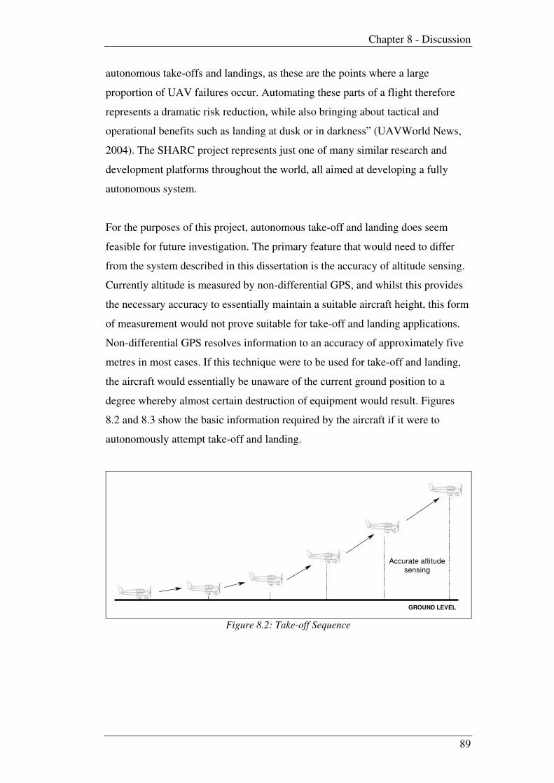
Chapter 8 - Discussion
89
autonomous take-offs and landings, as these are the points where a large
proportion of UAV failures occur. Automating these parts of a flight therefore
represents a dramatic risk reduction, while also bringing about tactical and
operational benefits such as landing at dusk or in darkness” (UAVWorld News,
2004). The SHARC project represents just one of many similar research and
development platforms throughout the world, all aimed at developing a fully
autonomous system.
For the purposes of this project, autonomous take-off and landing does seem
feasible for future investigation. The primary feature that would need to differ
from the system described in this dissertation is the accuracy of altitude sensing.
Currently altitude is measured by non-differential GPS, and whilst this provides
the necessary accuracy to essentially maintain a suitable aircraft height, this form
of measurement would not prove suitable for take-off and landing applications.
Non-differential GPS resolves information to an accuracy of approximately five
metres in most cases. If this technique were to be used for take-off and landing,
the aircraft would essentially be unaware of the current ground position to a
degree whereby almost certain destruction of equipment would result. Figures
8.2 and 8.3 show the basic information required by the aircraft if it were to
autonomously attempt take-off and landing.
GROUND LEVEL
Accurate altitude
sensing
Figure 8.2: Take-off Sequence

Chapter 8 - Discussion
90
Accurate altitude
sensing
GROUND LEVEL
Figure 8.3: Landing Sequence
So the fundamental component of autonomous take-off and landing is the need
for accurate altitude sensing so that the aircraft knows precisely where the
ground is during take-off and landing sequences. To achieve this accuracy, a
relatively low cost sensor unit has been identified. The SensComp 6500 Series
Ranging Module (previously manufactured by Polaroid) is an economical sonar
based ranging module that accurately measures altitudes from 6 inches to 35 feet
(SensComp Inc, 2004). This module was initially investigated as a sensor for the
actual altitude information for the purposes of this project; however for this
purpose its maximum range of 35 feet was inadequate. However for the purposes
of take-off and landing sequences the module would be more suited. Further
specifications for the 6500 Ranging Module are shown in appendix E.
Whilst the details mentioned in this section in regards to autonomous take-off
and landing are simply a very small representation of the level of research and
further investigation required, it does appear that the development of a fully
autonomous system may well be possible in future projects. Software details
have not yet been explored and it can be expected that the addition of this extra
autonomy feature will increase the complexities of the control platform. The
need for accuracy becomes fundamental in the design of autonomous take-off
and landing sequences and therefore it is recommended that if such a system is to
be implemented, then extensive testing should be carried out before any flight
tests are conducted. Overall it does appear that fully autonomous flight could be
an interesting and indeed a feasible future addition to this project.

Chapter 8 - Discussion
91
8.5 Final Word
The field of autonomous UAV research is a rapidly growing area, particularly at
the low budget university level. Future prospects and applications for these forms
of autonomous systems are continuing to increase, with continued emphasis on
the development of low cost systems for non-military applications. This project
has provided the initial building blocks for further research in this area at an
undergraduate level. The opportunity to combine theoretical research with
practical software and hardware development significantly adds to the
attractiveness of pursuing a future project in this topic. Expansion and
development opportunities for this project are significant and it is hoped that
students will continue take up this challenge for many years to come with the
hope of developing the optimal low cost autonomous UAV system.
92
References
Analog Devices Inc. 1999, 'Low Cost 2g/10g Dual Axis iMEMS Accelerometers
with Digital Output', Norwood, MA.
Beard, R, Kingston, D, Quigley 2003, M, Autonomous Vehicle Technologies for
Small Fixed Wing UAVS, Available [http://www.ee.byu.edu], (21 March 2005)
Byrne, T. 2005, 'Model Aircraft Specifications', ed. C Littleton, USQ,
Toowoomba
Byrne, T. 2005, 'M68HC12 Assembly Language Programming', ed. C Littleton,
USQ, Toowoomba
Civil Aviation Safety Authority 1998, Civil Aviation Safety Regulations 1998
(CASR 1998), Available [http://casa.gov.au/rules/index.htm], (21 May 2005)
Dallas Personal Robotics Group (DPRG) 2003, Low Cost Gyro-Accelerometer
Combo Sensor, Available [http://www.dprg.org/projects/2003-01a/], (18 March
2005)
Electronic Circuits Study Book, 2002, Distance Education Centre, USQ,
Toowoomba, Australia
Elektronikladen 2005, ‘Card 12; HC12 Controller Module with
MC912D60A/MC912DG128A’, Detmold, Germany
Franklin, G, Powell, J. 1994, Feedback Control of Dynamic Systems, Addison-
Wesley, USA
Gabrynowicz, Prof. J.I 2003, Legal Issues Using Satellite, Aerial and UAV
Platforms, National Remote Sensing and Space Law Centre, University of
Mississippi School of Law, MI
Garmin 2004, GPS 35 Specifications, Available
[http://www.garmin.com/products/gps35/spec.html], (1 March 2005)
Goebel, G 2005, Greg Goebel / In the Public Domain, Available
[http://www.vectorsite.net/index.html], (14 April 2005)
Institution of Engineers Australia 1997, Towards Sustainable Engineering
Practice: Engineering Frameworks for Sustainability, IEAUST, Australia
Institution of Engineers Australia 2000, 2000 Code of Ethics, IEAUST, Australia
Keeffe, M 2003, The Autonomous Scale Model Surveillance Aircraft,
Undergraduate, University of Southern Queensland, Toowoomba

93
Lazarski, Lt. Col. A.J 2002, ‘Legal implications of the uninhabited combat aerial
vehicle - Focus: Unmanned Aerial Vehicles’, Aerospace Power Journal,
Summer 2002, Available [http://www.findarticles.com]
MacQueen A.S 2002, Autonomous Scale Yacht, Undergraduate, University of
Southern Queensland, Toowoomba
McLean, D 1990, Automatic Flight Control Systems, Prentice Hall, United
Kingdom
Motorola 2002, M68HC12 & HCS12 Microcontrollers; CPU 12 Reference
Manual, Rev. 3 5/2002, Motorola Inc, Colorado
Motorola 2000, 68HC912D60 68HC12D60 Advance Information, Rev 2,
Motorola Inc, Colorado
Nise, N.S 2000, Control Systems Engineering 3rd
Edition, John Wiley and Sons,
Inc, New York
Ogata, K 1995, Discrete-Time Control Systems 2nd
Edition, Prentice Hall, New
Jersey
Phythian, M. 2003, Embedded Systems Design Study Book, Distance Education
Centre, USQ, Toowoomba, Australia
Precision Navigation Inc (n.d), Vector 2X and 2XG Electronic Compass Modules;
Complete Application Notes, Available [https://www.pnicorp.com/], (1 March
2005)
Senscomp Inc. 2004, '6500 Series Ranging Modules’, Livonia, MI.
Sindahl, L 2004, ‘SHARC completes autonomous take-off/landing’, UAVWorld
News, 26 October 2004, Available
[http://www.uavworld.com/_disc4/0000007c.htm]

94
APPENDIX A
Project Specification

University of Southern Queensland
FACULTY OF ENGINEERING AND SURVEYING
ENG4111/4112 Research Project
PROJECT SPECIFICATION
NAME: Craig Andrew LITTLETON
DEGREE: Bachelor of Engineering – Electrical and Electronic
Bachelor of Business – Operations and Logistics
Management
TITLE: Autonomous Unmanned Aerial Surveillance Vehicle –
Autonomous Control and Flight Dynamics
SUPERVISORS: Mr. Mark Phythian
ENROLMENT: ENG4111 – S1, 2005 (ONC)
ENG4112 – S2, 2005 (ONC)
PROJECT AIM: The ultimate goal of this project, (when integrated with
“Navigation and User Interface” (Soz Knox), is to develop
a fully functional prototype autonomous unmanned aerial
vehicle (UAV) to conduct specific flight path surveillance.
This particular project focuses on the autonomous flight
control aspect of the UAV system based on the dynamics
of flight.
PROGRAMME: Issue A, 21 March 2003
1. Research into various control methods currently employed in similar UAV
systems including relevant components.
2. Select, interface and test hardware components required for autonomous
capability.
3. Design and simulate control system algorithms required for autonomous
flight.
4. Construct prototype UAV (using a model aircraft) and integrate flight control
system with “Navigation and User Interface” being carried out by Soz Knox.
As time permits:
1. Examine the viability of developing control algorithms for autonomous take-
off and landing sequences.
AGREED:
_________________ (Student) _________________ (Supervisor)
__ / __ /2005 __ / __ /2005

96
APPENDIX B
Exert from Civil Aviation Safety Regulations act of 1998
(CASA, 2004)

Subpart 101.A Preliminary
101.025 Meaning of populous area
For this Part, an area is a populous area in relation to the operation of an
unmanned aircraft or rocket if the area has a sufficient density of
population for some aspect of the operation, or some event that might
happen during the operation (in particular, a fault in, or failure of, the
aircraft or rocket) to pose an unreasonable risk to the life, safety or
property of somebody who is in the area but is not connected with the
operation.
101.030 Approval of areas for operation of unmanned aircraft or rockets
(1) A person may apply to CASA for the approval of an area as an area
for the operation of:
(a) unmanned aircraft generally, or a particular class of unmanned
aircraft; or
(b) rockets.
(2) For paragraph (1) (a), the classes of unmanned aircraft are the
following:
(a) tethered balloons and kites;
(b) unmanned free balloons;
(c) UAVs;
(d) model aircraft.
(3) In considering whether to approve an area for any of those purposes,
CASA must take into account the likely effect on the safety of air navigation of
the operation of unmanned aircraft in, or the launching of rockets in or over, the
area.
(4) An approval has effect from the time written notice of it is given to
the applicant, or a later day or day and time stated in the approval.
(5) An approval may be expressed to have effect for a particular period
(including a period of less than 1 day), or indefinitely.
(6) CASA may impose conditions on the approval in the interests of the
safety of air navigation.
(7) If CASA approves an area under subregulation (1), it must publish
details of the approval (including any condition) in NOTAM or on an
aeronautical chart.
(8) CASA may revoke the approval of an area, or change the conditions
that apply to such an approval, in the interests of the safety of air navigation, but
must publish details of any revocation or change in NOTAM or on an
aeronautical chart.
(9) CASA must also give written notice of the revocation or change:
(a) to the person who applied for the approval of the area; or
(b) if that person applied for that approval as an officer of an
organisation concerned with unmanned aircraft or rockets, and no
longer holds that office — to the person who now holds the office.

Subpart 101.C Provisions applicable to unmanned aircraft Generally 101.060 Applicability of this Subpart
This Subpart applies to the operation of unmanned aircraft of all kinds,
except operation mentioned in subregulation 101.005 (3). Note Rockets that are not aircraft are dealt with separately in Subpart 101.H.
101.065 Operation in prohibited or restricted area (1) A person may operate an unmanned aircraft in or over a prohibited
area, or in or over a restricted area, only with the permission of, and in
accordance with any conditions imposed by, the authority controlling the area.
Penalty: 25 penalty units. Note For prohibited area and restricted area, see regulation 2.07 of the Air Services Regulations.
Details of prohibited or restricted areas are published in AIP or NOTAM.
(1A) An offence against subregulation (1) is an offence of strict liability. Note For strict liability, see section 6.1 of the Criminal Code.
(2) In subregulation (1):
authority controlling the area means:
(a) in the case of a prohibited area — the Secretary to the
Department of Defence; and
(b) in the case of a restricted area — the authority mentioned in
AIP (as issued from time to time) as the controlling authority for
the area.
(3) For subregulation (1):
(a) the authority controlling the area must give a written statement
of any condition so imposed to the person who applied for the
permission; and
(b) unless the authority gives the statement to the person, the
person is not bound by the condition.
101.070 Operation in controlled airspace (1) A person may operate an unmanned aircraft above 400 feet AGL in
controlled airspace only:
(a) in an area approved under regulation 101.030 as an area for the
operation of unmanned aircraft of the same kind as the aircraft,
and in accordance with any conditions of the approval; and
(b) in accordance with an air traffic control clearance.
Penalty: 50 penalty units. Note AGL = above ground level (see the Dictionary).
(2) An offence against subregulation (1) is an offence of strict liability. Note For strict liability, see section 6.1 of the Criminal Code.
101.075 Operation near aerodromes
(1) A person may operate an unmanned aircraft at an altitude above 400
feet AGL within 3 nautical miles of an aerodrome only if:
(a) the operation is permitted by another provision of this Part; or
(b) permission has been given for the operation under regulation
101.080.
Penalty: 25 penalty units.

Note AGL = above ground level (see the Dictionary).
(2) A person may operate an unmanned aircraft over an area mentioned in
paragraph (3) (a) or (b) only if:
(a) the operation is permitted by another provision of this Part; or
(b) permission has been given for the operation under regulation
101.080.
Penalty: 25 penalty units.
(3) The areas for subregulation (2) are:
(a) a movement area or runway of an aerodrome; and
(b) the approach or departure path of a runway of an aerodrome.
(4) A person must not operate an unmanned aircraft in such a manner as
to create an obstruction to an aircraft taking off from, or approaching for landing
at, a landing area or a runway of an aerodrome.
Penalty: 25 penalty units.
(5) An offence against subregulation (1), (2) or (4) is an offence of strict
liability. Note For strict liability, see section 6.1 of the Criminal Code.
101.080 Permission for operation of unmanned aircraft near aerodrome
(1) The authority from which permission must be obtained for the
purposes of regulation 101.075 is:
(a) if the aerodrome concerned is a controlled aerodrome — the
air traffic control service for the aerodrome; or
(b) in the case of any other aerodrome — CASA.
(2) A person applies for permission under this regulation by giving to the
relevant authority mentioned in subregulation (1) the information required by
table 101.080, so far as relevant to the proposed operation.
Table 101.080 Details of operation of unmanned aircraft to be given to CASA or ATC Item Information to be provided
1 In all cases:
(a) the name, address and telephone number of the person who will operate the
aircraft or (if the aircraft concerned is an unmanned free balloon) release the balloon (or,
if several people will be involved, the name, address and telephone number of the person
who will coordinate the operation); and
(b) the date and time the operation or release is to begin and how long it is to
last; and
(c) where it is to be carried out; and
(d) if more than 1 unmanned aircraft is to be operated at a time, how many
unmanned aircraft are to be operated at that time
2 In the case of the operation of a tethered balloon or a kite:
(a) a brief description of the balloon or kite, including its predominant colour;
and
(b) the height to which it is to be operated; and
(c) its mass
3 In the case of the release of a free balloon:
(a) how many balloons are to be released; and
(b) the estimated size and mass of the balloon’s payload
4 In the case of the release of a medium or heavy balloon:
(a) the balloon’s flight identification or its project code name; and
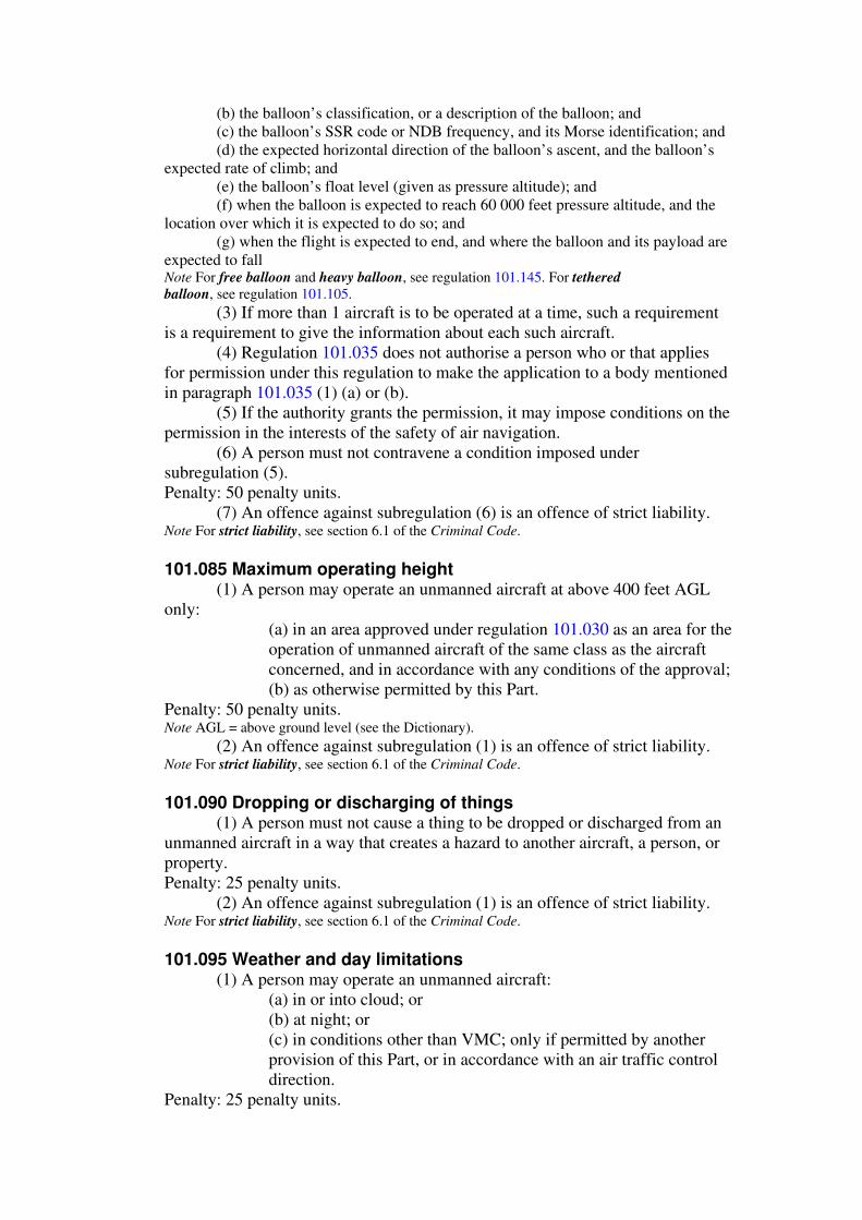
(b) the balloon’s classification, or a description of the balloon; and
(c) the balloon’s SSR code or NDB frequency, and its Morse identification; and
(d) the expected horizontal direction of the balloon’s ascent, and the balloon’s
expected rate of climb; and
(e) the balloon’s float level (given as pressure altitude); and
(f) when the balloon is expected to reach 60 000 feet pressure altitude, and the
location over which it is expected to do so; and
(g) when the flight is expected to end, and where the balloon and its payload are
expected to fall Note For free balloon and heavy balloon, see regulation 101.145. For tethered
balloon, see regulation 101.105.
(3) If more than 1 aircraft is to be operated at a time, such a requirement
is a requirement to give the information about each such aircraft.
(4) Regulation 101.035 does not authorise a person who or that applies
for permission under this regulation to make the application to a body mentioned
in paragraph 101.035 (1) (a) or (b).
(5) If the authority grants the permission, it may impose conditions on the
permission in the interests of the safety of air navigation.
(6) A person must not contravene a condition imposed under
subregulation (5).
Penalty: 50 penalty units.
(7) An offence against subregulation (6) is an offence of strict liability. Note For strict liability, see section 6.1 of the Criminal Code.
101.085 Maximum operating height
(1) A person may operate an unmanned aircraft at above 400 feet AGL
only:
(a) in an area approved under regulation 101.030 as an area for the
operation of unmanned aircraft of the same class as the aircraft
concerned, and in accordance with any conditions of the approval;
(b) as otherwise permitted by this Part.
Penalty: 50 penalty units. Note AGL = above ground level (see the Dictionary).
(2) An offence against subregulation (1) is an offence of strict liability. Note For strict liability, see section 6.1 of the Criminal Code.
101.090 Dropping or discharging of things
(1) A person must not cause a thing to be dropped or discharged from an
unmanned aircraft in a way that creates a hazard to another aircraft, a person, or
property.
Penalty: 25 penalty units.
(2) An offence against subregulation (1) is an offence of strict liability. Note For strict liability, see section 6.1 of the Criminal Code.
101.095 Weather and day limitations
(1) A person may operate an unmanned aircraft:
(a) in or into cloud; or
(b) at night; or
(c) in conditions other than VMC; only if permitted by another
provision of this Part, or in accordance with an air traffic control
direction.
Penalty: 25 penalty units.
(2) An offence against subregulation (1) is an offence of strict liability.
Subpart 101.F UAVs Division 101.F.1 General 101.235 Applicability of this Subpart
(1) This Subpart applies to:
(a) the operation of a large UAV; and
(b) the operation of a small UAV for purposes other than sport or
recreation. Note 1 There is no practicable distinction between a small UAV and a model aircraft except that
of use — model aircraft are flown only for the sport of flying them.
Note 2 For large UAV and small UAV, see regulation 101.240. For model aircraft see the
Dictionary.
(2) Nothing in this Subpart applies to the operation of a UAV if:
(a) while it is being operated, the person operating it keeps it in
sight; and
(b) it is operated in a way that complies with Subpart 101.G.
(3) This Subpart does not apply to the operation of a micro UAV. Note 1 See subregulation 101.005 (3).
Note 2 For micro UAV, see regulation 101.240.
101.240 Definitions for Subpart In this Subpart:
approved area means an area approved under regulation 101.030 as an
area for the operation of UAVs. Note CASA must publish details of the approval of an area (including any
conditions) in NOTAM or on an aeronautical chart — see
subregulation 101.030 (5).
certified UAV controller means a person certified under Division 3 as a
controller of UAVs.
controller of a UAV means a person who performs a function that would
be, if the UAV were a manned aircraft, a function of its flight crew.
large UAV means any of the following:
(a) an unmanned airship with an envelope capacity greater than
100 cubic metres;
(b) an unmanned powered parachute with a launch mass greater
than 150 kilograms;
(c) an unmanned aeroplane with a launch mass greater than 150
kilograms;
(d) an unmanned rotorcraft with a launch mass greater than 100
kilograms;
(e) an unmanned powered lift device with a launch mass greater
than 100 kilograms.
micro UAV means a UAV with a gross weight of 100 grams or less.
small UAV means a UAV that is not a large UAV nor a micro UAV.
UAV means unmanned aircraft, other than a balloon or a kite.
Division 101.F.2 Operation of UAVs generally 101.245 Operation near people

(1) Subject to subregulations (2) and (3), a person must not operate a
UAV within 30 metres of a person who is not directly associated with the
operation of the UAV.
Penalty: 10 penalty units.
(1A) An offence against subregulation (1) is an offence of strict liability. Note For strict liability, see section 6.1 of the Criminal Code.
(2) Subregulation (1) does not apply in relation to a person who stands
behind the UAV while it is taking off.
(3) Subregulation (1) also does not prevent the operation of a UAV
airship within 30 metres of a person if the airship approaches no closer to the
person than 10 metres horizontally and 30 feet vertically.
101.250 Where small UAVs may be operated
(1) A person may operate a small UAV outside an approved area only if:
(a) where the UAV is operated above 400 feet AGL, the operator
has CASA’s approval to do so; and
(b) the UAV stays clear of populous areas.
Penalty: 10 penalty units. Note 1 AGL = above ground level (see the Dictionary). For populous area, see
regulation 101.025. For small UAV, see regulation 101.240.
Note 2 CASA must publish details of the approval of an area (including any
conditions) in NOTAM or on an aeronautical chart — see
subregulation 101.030 (5).
Note 3 For the kinds of UAV operation to which this Subpart does not apply, see
regulation 101.235.
(2) An offence against subregulation (1) is an offence of strict liability. Note For strict liability, see section 6.1 of the Criminal Code.
101.280 UAVs not to be operated over populous areas (1) In this regulation:
certificated UAV means a UAV for which a certificate of airworthiness
has been issued.
(2) A person must not operate a UAV that is not a certificated UAV over
a populous area at a height less than the height from which, if any of its
components fails, it would be able to clear the area.
Penalty: 50 penalty units. Note 1 For populous area, see regulation 101.025. For UAV, see regulation
101.240.
Note 2 For the kinds of UAV operation to which this Subpart does not apply, see
regulation 101.235.
(3) Without the approval of CASA, a person must not operate a
certificated UAV over a populous area at a height less than the height from
which, if any of its components fails, it would be able to clear the area.
Penalty: 50 penalty units.
(3A) An offence against subregulation (2) or (3) is an offence of strict
liability. Note For strict liability, see section 6.1 of the Criminal Code.
(4) In considering whether to give an approval under subregulation (3),
CASA must take into account:
(a) the degree of redundancy in the UAV’s critical systems; and
(b) any fail-safe design characteristics of the UAV; and
(c) the security of its communications and navigation systems.

(5) Before giving an approval under subregulation (3), CASA must be
satisfied that the person who intends to operate the UAV will take proper
precautions to prevent the proposed flight being dangerous to people and
property.
Subpart 101.G Model aircraft 101.375 Applicability of this Subpart This Subpart applies to the operation of model aircraft weighing 100
grams or more (except operation mentioned in paragraph
101.005 (3) (a) or (b)).
101.385 Visibility for operation of model aircraft (1) A person may operate a model aircraft only if the visibility at the time
is good enough for the person operating the model to be able to see it
continuously.
Penalty: 25 penalty units.
(2) An offence against subregulation (1) is an offence of strict liability. Note For strict liability, see section 6.1 of the Criminal Code.
101.390 Operating model aircraft at night
(1) A person may operate a model aircraft at night only in accordance
with the written procedures of an approved aviation administration organisation.
Penalty: 25 penalty units.
(2) An offence against subregulation (1) is an offence of strict liability. Note For strict liability, see section 6.1 of the Criminal Code.
101.395 Keeping model aircraft away from people (1) A person must not operate a model aircraft over a populous area at a
height less than the height from which, if any of its components fails, it would be
able to clear the area.
Penalty: 50 penalty units. Note For populous area, see regulation 101.025.
(2) Subject to subregulations (3) and (4), somebody who is operating a
powered model aircraft must ensure that, while the model aircraft is in flight, or
is landing or taking off, it stays at least 30 metres away from anyone not directly
associated with the operation of model aircraft.
Penalty: 50 penalty units.
(3) Subregulation (2) is not contravened if somebody stands behind the
model aircraft while it is taking off.
(4) Subregulation (2) is also not contravened if, as part of a model flying
competition, a model aircraft is flown within 30 metres of somebody who is
judging the competition.
(5) An offence against subregulation (1) or (2) is an offence of strict
liability. Note For strict liability, see section 6.1 of the Criminal Code.

104
APPENDIX C
MATLAB Simulation Files
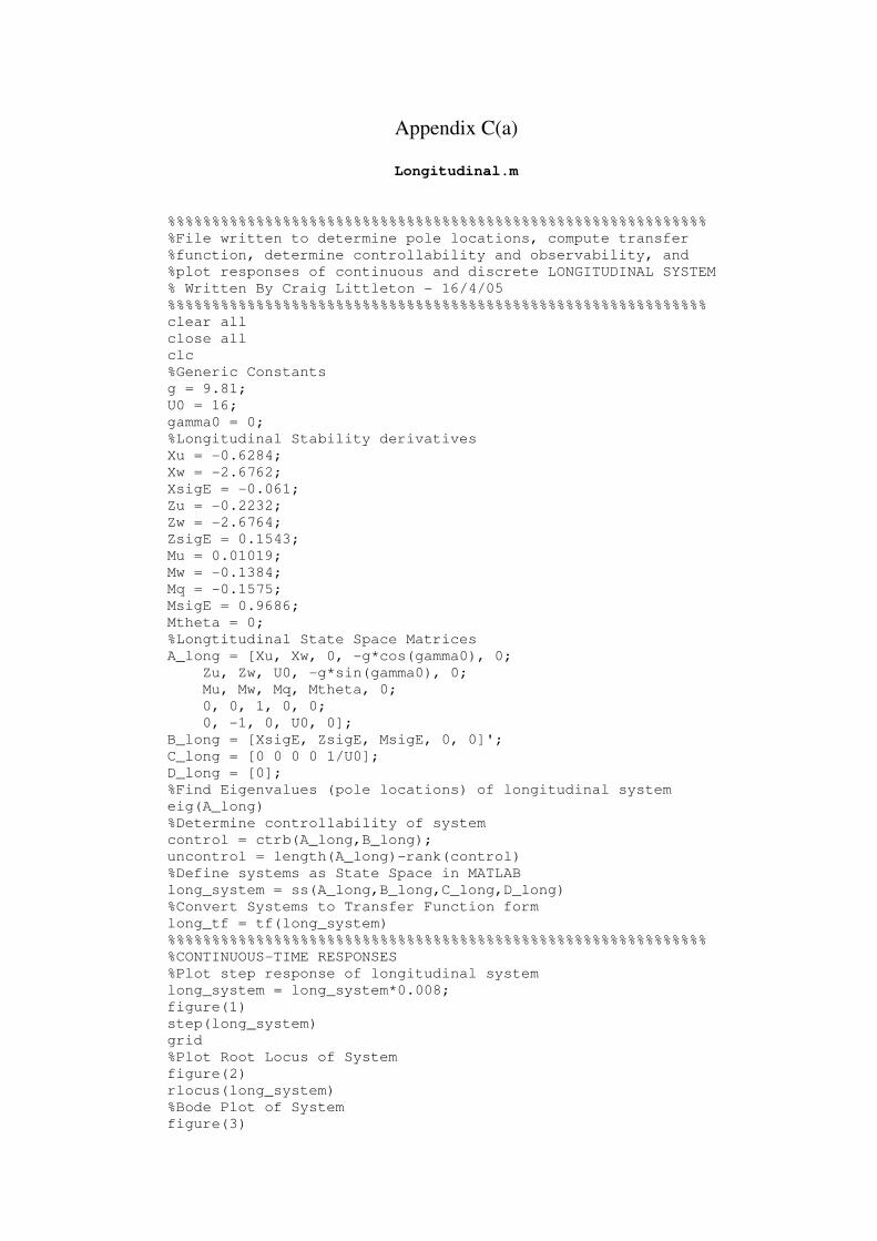
Appendix C(a)
Longitudinal.m
%%%%%%%%%%%%%%%%%%%%%%%%%%%%%%%%%%%%%%%%%%%%%%%%%%%%%%%%%%%%%
%File written to determine pole locations, compute transfer
%function, determine controllability and observability, and
%plot responses of continuous and discrete LONGITUDINAL SYSTEM
% Written By Craig Littleton - 16/4/05
%%%%%%%%%%%%%%%%%%%%%%%%%%%%%%%%%%%%%%%%%%%%%%%%%%%%%%%%%%%%%
clear all
close all
clc
%Generic Constants
g = 9.81;
U0 = 16;
gamma0 = 0;
%Longitudinal Stability derivatives
Xu = -0.6284;
Xw = -2.6762;
XsigE = -0.061;
Zu = -0.2232;
Zw = -2.6764;
ZsigE = 0.1543;
Mu = 0.01019;
Mw = -0.1384;
Mq = -0.1575;
MsigE = 0.9686;
Mtheta = 0;
%Longtitudinal State Space Matrices
A_long = [Xu, Xw, 0, -g*cos(gamma0), 0;
Zu, Zw, U0, -g*sin(gamma0), 0;
Mu, Mw, Mq, Mtheta, 0;
0, 0, 1, 0, 0;
0, -1, 0, U0, 0];
B_long = [XsigE, ZsigE, MsigE, 0, 0]';
C_long = [0 0 0 0 1/U0];
D_long = [0];
%Find Eigenvalues (pole locations) of longitudinal system
eig(A_long)
%Determine controllability of system
control = ctrb(A_long,B_long);
uncontrol = length(A_long)-rank(control)
%Define systems as State Space in MATLAB
long_system = ss(A_long,B_long,C_long,D_long)
%Convert Systems to Transfer Function form
long_tf = tf(long_system)
%%%%%%%%%%%%%%%%%%%%%%%%%%%%%%%%%%%%%%%%%%%%%%%%%%%%%%%%%%%%%
%CONTINUOUS-TIME RESPONSES
%Plot step response of longitudinal system
long_system = long_system*0.008;
figure(1)
step(long_system)
grid
%Plot Root Locus of System
figure(2)
rlocus(long_system)
%Bode Plot of System
figure(3)

margin(long_system)
figure(4)
bode(long_system)
%Impulse Response of System
figure(5)
impulse(long_system)
grid
damp(long_system)
pause
close all
%%%%%%%%%%%%%%%%%%%%%%%%%%%%%%%%%%%%%%%%%%%%%%%%%%%%%%%%%%%%%
%SYSTEM DISCRETIZATION AND DISCRETE RESPONSES
Ts = 0.625;
[phi,gamma] = c2d(A_long,B_long,Ts);
gamma = gamma*0.008;
%Plot step response of longitudinal system
figure(1)
dstep(phi,gamma,C_long,D_long)
grid
%Plot Root Locus of System
figure(2)
rlocus(phi,gamma,C_long,D_long)
%Bode Plot of System
figure(3)
bode(phi,gamma,C_long,D_long)
%Impulse Response of System
figure(4)
dimpulse(phi,gamma,C_long,D_long)
grid
pause
close all
%EOF
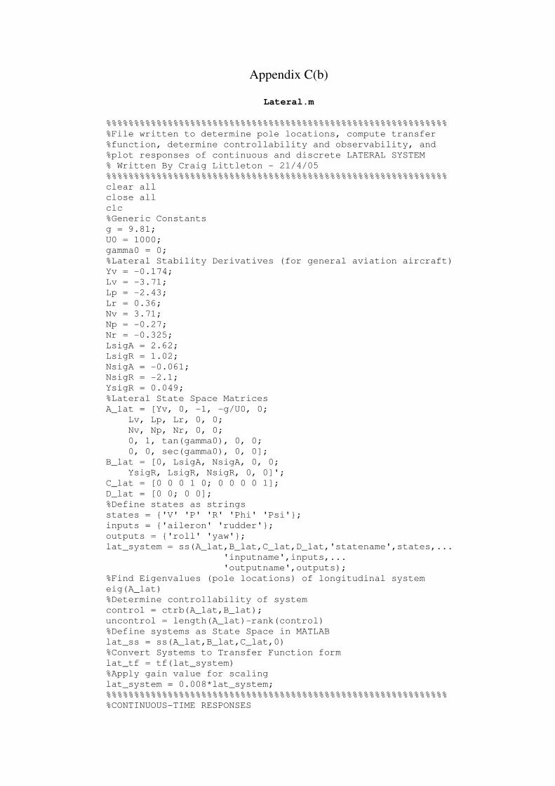
Appendix C(b)
Lateral.m
%%%%%%%%%%%%%%%%%%%%%%%%%%%%%%%%%%%%%%%%%%%%%%%%%%%%%%%%%%%%%
%File written to determine pole locations, compute transfer
%function, determine controllability and observability, and
%plot responses of continuous and discrete LATERAL SYSTEM
% Written By Craig Littleton - 21/4/05
%%%%%%%%%%%%%%%%%%%%%%%%%%%%%%%%%%%%%%%%%%%%%%%%%%%%%%%%%%%%%
clear all
close all
clc
%Generic Constants
g = 9.81;
U0 = 1000;
gamma0 = 0;
%Lateral Stability Derivatives (for general aviation aircraft)
Yv = -0.174;
Lv = -3.71;
Lp = -2.43;
Lr = 0.36;
Nv = 3.71;
Np = -0.27;
Nr = -0.325;
LsigA = 2.62;
LsigR = 1.02;
NsigA = -0.061;
NsigR = -2.1;
YsigR = 0.049;
%Lateral State Space Matrices
A_lat = [Yv, 0, -1, -g/U0, 0;
Lv, Lp, Lr, 0, 0;
Nv, Np, Nr, 0, 0;
0, 1, tan(gamma0), 0, 0;
0, 0, sec(gamma0), 0, 0];
B_lat = [0, LsigA, NsigA, 0, 0;
YsigR, LsigR, NsigR, 0, 0]';
C_lat = [0 0 0 1 0; 0 0 0 0 1];
D_lat = [0 0; 0 0];
%Define states as strings
states = {'V' 'P' 'R' 'Phi' 'Psi'};
inputs = {'aileron' 'rudder'};
outputs = {'roll' 'yaw'};
lat_system = ss(A_lat,B_lat,C_lat,D_lat,'statename',states,...
'inputname',inputs,...
'outputname',outputs);
%Find Eigenvalues (pole locations) of longitudinal system
eig(A_lat)
%Determine controllability of system
control = ctrb(A_lat,B_lat);
uncontrol = length(A_lat)-rank(control)
%Define systems as State Space in MATLAB
lat_ss = ss(A_lat,B_lat,C_lat,0)
%Convert Systems to Transfer Function form
lat_tf = tf(lat_system)
%Apply gain value for scaling
lat_system = 0.008*lat_system;
%%%%%%%%%%%%%%%%%%%%%%%%%%%%%%%%%%%%%%%%%%%%%%%%%%%%%%%%%%%%%
%CONTINUOUS-TIME RESPONSES

%Plot step response of lateral system
figure(1)
step(lat_system)
%Bode Plot of System
figure(2)
bode(lat_system)
%Impulse Response of System
figure(3)
impulse(lat_system)
pause
close all
%%%%%%%%%%%%%%%%%%%%%%%%%%%%%%%%%%%%%%%%%%%%%%%%%%%%%%%%%%%%%
%SYSTEM DISCRETIZATION AND DISCRETE RESPONSES
Ts = 0.564;
[phi,gamma] = c2d(A_lat,B_lat,Ts);
%Plot step response of discrete lateral system
figure(1)
dstep(phi,gamma,C_lat,D_lat)
%Bode Plot of discrete system
figure(2)
bode(phi,gamma,C_lat,D_lat)
%Impulse Response of discrete system
figure(3)
dimpulse(phi,gamma,C_lat,D_lat)
pause
close
%EOF

109
APPENDIX D
MC912D60A HC12 Microcontroller Assembly Language Control
Algorithms

Appendix D(a)
Remote.a
CPU 68HC12
PADDING OFF
COPCTL equ $16 ;COP Control
TIOS equ $80 ;Timer Input Capture/Output Compare Select
CFORC equ $81 ;Timer Compare Force
TSCR equ $86 ;Timer System Control
TCTL2 equ $89 ;Timer Control 2
TCTL3 equ $8A ;Timer Control 3
TFLG1 equ $8E ;Timer Interrupt Flag 1
TC4 equ $98 ;TIC/TOC 4
SC0BDH equ $C0 ;SCI 0 Baud Rate
SC0CR2 equ $C3 ;SCI 0 Control 2
RAMTOP equ $0600 ;Top of usable RAM
RAMTOPMON equ $07FF ;Top of RAM used by monitor
CODE equ $8000
ORG $0200
HIVAL RMB 3
HEXVAL RMB 1
;================================================================
; START OF MAIN PROGRAMME
ORG CODE
main lds #RAMTOP ;Stack Pointer
clr COPCTL ;Disable COP Watchdog
jsr serial_init ;Setup serial port
jsr SETUP_ICOC ;Setup i/p capture and o/p compare
loop1 jsr PWM_REC ;Decodes pulse width from remote
;transmitter
bra loop1
;****************************************************************
;Setup input capture and output compare
SETUP_ICOC
ldaa #%10010000 ;Timer to operate normally (p188) and
staa TSCR ;enable fast clear of TC flag
ldaa #%00001100 ;1->Output 0->Input (p185)
staa TIOS ;Channel 0/1 - accel i/p; Channel 2/3 –
;servo o/p; Channel 4/5 - remote i/
RTS
;****************************************************************
;Decode PWM signal from accelerometer and control enable servo
pulses
PWM_REC
ldaa #%00000001 ;i/p capture on line 4 on rising edge
staa TCTL3
ldd TC4 ;clears flag
ldaa #%00110000 ;Sets up to set o/p compare line 2 to
;'high' on successful compare (p190)
staa TCTL2
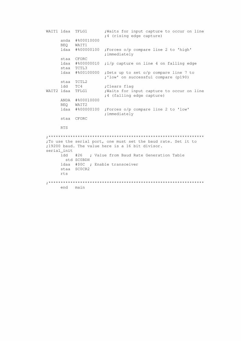
WAIT1 ldaa TFLG1 ;Waits for input capture to occur on line
;4 (rising edge capture)
anda #%00010000
BEQ WAIT1
ldaa #%00000100 ;Forces o/p compare line 2 to 'high'
;immediately
staa CFORC
ldaa #%00000010 ;i/p capture on line 4 on falling edge
staa TCTL3
ldaa #%00100000 ;Sets up to set o/p compare line 7 to
;'low' on successful compare (p190)
staa TCTL2
ldd TC4 ;Clears flag
WAIT2 ldaa TFLG1 ;Waits for input capture to occur on line
;4 (falling edge capture)
ANDA #%00010000
BEQ WAIT2
ldaa #%00000100 ;Forces o/p compare line 2 to 'low'
;immediately
staa CFORC
RTS
;****************************************************************
;To use the serial port, one must set the baud rate. Set it to
;19200 baud. The value here is a 16 bit divisor.
serial_init
ldd #26 ; Value from Baud Rate Generation Table
std SC0BDH
ldaa #$0C ; Enable transceiver
staa SC0CR2
rts
;****************************************************************
end main

Appendix D(b)
Servo.a
CPU 68HC12
PADDING OFF
RTICTL equ $14 ;Real Time Interrupt Control
RTIFLG equ $15 ;Real Time Interrupt Flag
COPCTL equ $16 ;COP Control
TIOS equ $80 ;Timer Input Capture/Output Compare Select
CFORC equ $81 ;Timer Compare Force
TCNT equ $84 ;Timer Counter
TSCR equ $86 ;Timer System Control
TCTL1 equ $88 ;Timer Control 1
TC7 equ $9E ;TIC/TOC 7
SC0BDH equ $C0 ;SCI 0 Baud Rate
SC0CR2 equ $C3 ;SCI 0 Control 2
RAMTOP equ $0600 ;Top of usable RAM
RAMTOPMON equ $07FF ;Top of RAM used by monitor
CODE equ $8000
ORG $0200
SERVO1 RMB 2
;================================================================
; START OF MAIN PROGRAMME
ORG CODE
main lds #RAMTOP ;Stack Pointer
clr COPCTL ;Disable COP Watchdog
jsr serial_init ; Setup serial port
jsr SET_RTI
loop nop
bra loop
;****************************************************************
; To use the serial port, one must set the baud rate. Set it to
;19200 baud. The value here is a 16 bit divisor.
serial_init
ldd #26 ; Value from Baud Rate Generation Table
std SC0BDH
ldaa #$0C ; Enable transceiver
staa SC0CR2
RTS
;****************************************************************
; SETUP RTI for servos
SET_RTI
jsr RTI_SETUP
jsr SETUP_OUTCOM
ldd #12000 ;Pulse Width for Servo-> 1 count = 125nS
std servo1 ;12000 = 1.5mS = centre servo
RTS

;****************************************************************
;Setup Pseudo Interrupt Vectors as per Page 11-12 in Card12 User
;Manual
RTI_SETUP
ldaa #$06 ;JMP Command Opcode
staa $07EB ;RTI Pseudo Vector
ldd #RTI_SERVICE ;Address to jump, RTI Service
std $07EC
cli ;Clear interupt mask
ldaa #%10000110 ;Value to Setup RTI for an INT every 32mS
staa RTICTL ;Store Value in RTI Control Registe
ldaa #%10000000 ;Clear RTI Flag
staa RTIFLG
RTS
;***************************************************************
SETUP_OUTCOM
ldaa #%10000000
staa TSCR ;Timer to operate normally (p188)
ldaa #%10000000 ;1->Output 0->Input (p185)
staa TIOS ;Channel 7 as o/p --> 1-6 as i/p
RTS
;****************************************************************
;Real Time Interrupt Service Routine
;Manually sets output line, sets up automatic clearing of bit
;then loads required delay into Output Compare register
;When Main timer "TCNT" equals compare register bit is cleared
;automatically
RTI_SERVICE
ldaa #%10000000 ;Clear RTI Flag as time-out period is met
staa RTIFLG
ldaa #%11000000 ;Sets up to set o/p compare line 7 to
'high' on successful compare (p190)
staa TCTL1
ldaa #%10000000 ;Forces o/p compare line 7 to 'high’
immediately
staa CFORC
ldaa #%10000000 ;Sets up to set o/p compare line 7 to
'low' on successful compare (p190)
staa TCTL1
ldd TCNT ;Get value from Main Timer Counter
addd SERVO1 ;add required delay
std TC7 ;Store in Output Compare Register
;--> When main timer counts up to this
;value you get a successful compare which
;clears output pin (sets o/p compare line
;7 to 'low')
RTI ;Return from Interrupt
;****************************************************************
end main

Appendix D(c)
Pwm.a
CPU 68HC12
PADDING OFF
COPCTL equ $16 ;COP Control
TIOS equ $80 ;Timer Input Capture/Output Compare Select
TSCR equ $86 ;Timer System Control
TCTL4 equ $8B ;Timer Control 4
TFLG1 equ $8E ;Timer Interrupt Flag 1
TC0 equ $90 ;TIC/TOC 0
SC0BDH equ $C0 ;SCI 0 Baud Rate
SC0BDL equ $C1 ;SCI 0 Baud Rate Low Byte
SC0CR1 equ $C2 ;SCI 0 Control 1
SC0CR2 equ $C3 ;SCI 0 Control 2
SC0SR1 equ $C4 ;SCI 0 Status 1
SC0SR2 equ $C5 ;SCI 0 Status 2
SC0DRH equ $C6 ;SCI 0 Data
SC0DRL equ $C7 ;SCI 0 Data Low Byte
RAMTOP equ $0600 ;Top of usable RAM
RAMTOPMON equ $07FF ;Top of RAM used by monitor
CODE equ $8000
ORG $0200
TIME_1 RMB 2
TIME_2 RMB 2
TIME_3 RMB 2
PULSE_WIDTH RMB 2
PERIOD RMB 2
LEVEL_CYCLE RMB 2
ERROR RMB 2
DIRECTION RMB 1
HIVAL RMB 3
HEXVAL RMB 1
;================================================================
; START OF MAIN PROGRAMME
ORG CODE
main lds #RAMTOP ;Stack Pointer
clr COPCTL ;Disable COP Watchdog
jsr serial_init ;Setup serial port
jsr SETUP_INCAP
decode jsr PWM_DECODE ;Jump to decode routine
jsr CALC_DC ;Jump to error calculation routine
ldd ERROR ;Prints error results to terminal
;for verification
jsr PRINT_CHECK ;Jumps to terminal print routine
;****************************************************************
;Setup input capture
SETUP_INCAP
ldaa #%10010000 ;Timer to operate normally (p188) and
staa TSCR ;enable fast clear of TC flag
ldaa #%00001100 ;1->Output 0->Input (p185)

staa TIOS ;Channel 0/1 - accel i/p; Channel 2/3 –
;servo o/p; Channel 4/5 - remote i/p
RTS
;****************************************************************
;Decode PWM signal from accelerometer
PWM_DECODE
ldaa #%00000001 ;i/p capture on line 0 on rising edge
staa TCTL4
ldd TC0 ;clears flag
WAIT1 ldaa TFLG1 ;Waits for input capture to occur on line
;0 (rising edge capture)
anda #%00000001
BEQ WAIT1
ldaa #%00000010 ;i/p capture on line 0 on falling edge
staa TCTL4
ldd TC0 ;Retrieves timer value of rising edge (16
std TIME_1 ;bit) from IC register and stores to
;time_1, also clears TC flag
WAIT2 ldaa TFLG1 ;Waits for input capture to occur on line
;0 (falling edge capture)
ANDA #%00000001
BEQ WAIT2
ldaa #%00000001 ;i/p capture on line 0 on rising edge
staa TCTL4
ldd TC0 ;Retrieve timer value from falling
std TIME_2 ;trigger and store to time_2
subd TIME_1 ;also clears TC flag
std PULSE_WIDTH
WAIT3 ldaa TFLG1 ;Waits for input capture to occur on line
;0 (rising edge capture)
ANDA #%00000001
BEQ WAIT3
ldd TC0 ;Retrieve timer value from next rising
std TIME_3 ;trigger and store to time_3 also clears
;TC flag
subd TIME_1
std PERIOD
RTS
;**************************************************************
;Calculate duty cycle from recorded timer values
CALC_DC
ldd PERIOD
lsrd ;Divide period by 2 to get duty-
;cycle 50% (level flight)
std LEVEL_CYCLE
cpd PULSE_WIDTH
bls greater ;If result is negative, actual d/c
;is greater than desired d/c
subd PULSE_WIDTH ;Find difference between desired
;and actual duty cycle
std ERROR ;Store difference in d/c's (ie
;error) in ERROR
ldaa #%10000000 ;If actual d/c less than desired
;d/c then store 1 in MSB of
staa DIRECTION
bra difference
greater ldd PULSE_WIDTH ;Compute difference between pulse

;width and 50%
subd LEVEL_CYCLE
std ERROR
clra
staa DIRECTION ;If actual d/c greater than
;50% then store 0 in DIRECTION
difference RTS
;****************************************************************
; To use the serial port, one must set the baud rate. Set it to
19200
; baud. The value here is a 16 bit divisor.
serial_init
ldd #26 ; Value from Baud Rate Generation Table
std SC0BDH
ldaa #$0C ; Enable transceiver
staa SC0CR2
rts
;****************************************************************
end main
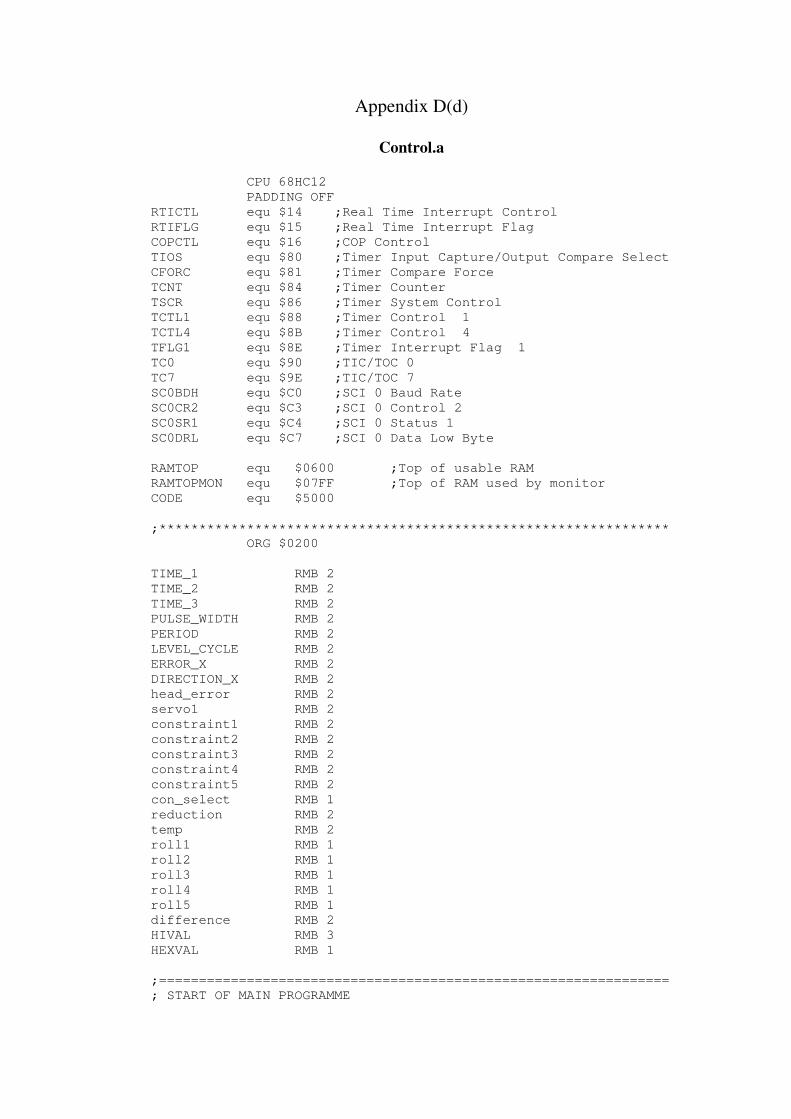
Appendix D(d)
Control.a
CPU 68HC12
PADDING OFF
RTICTL equ $14 ;Real Time Interrupt Control
RTIFLG equ $15 ;Real Time Interrupt Flag
COPCTL equ $16 ;COP Control
TIOS equ $80 ;Timer Input Capture/Output Compare Select
CFORC equ $81 ;Timer Compare Force
TCNT equ $84 ;Timer Counter
TSCR equ $86 ;Timer System Control
TCTL1 equ $88 ;Timer Control 1
TCTL4 equ $8B ;Timer Control 4
TFLG1 equ $8E ;Timer Interrupt Flag 1
TC0 equ $90 ;TIC/TOC 0
TC7 equ $9E ;TIC/TOC 7
SC0BDH equ $C0 ;SCI 0 Baud Rate
SC0CR2 equ $C3 ;SCI 0 Control 2
SC0SR1 equ $C4 ;SCI 0 Status 1
SC0DRL equ $C7 ;SCI 0 Data Low Byte
RAMTOP equ $0600 ;Top of usable RAM
RAMTOPMON equ $07FF ;Top of RAM used by monitor
CODE equ $5000
;****************************************************************
ORG $0200
TIME_1 RMB 2
TIME_2 RMB 2
TIME_3 RMB 2
PULSE_WIDTH RMB 2
PERIOD RMB 2
LEVEL_CYCLE RMB 2
ERROR_X RMB 2
DIRECTION_X RMB 2
head_error RMB 2
servo1 RMB 2
constraint1 RMB 2
constraint2 RMB 2
constraint3 RMB 2
constraint4 RMB 2
constraint5 RMB 2
con_select RMB 1
reduction RMB 2
temp RMB 2
roll1 RMB 1
roll2 RMB 1
roll3 RMB 1
roll4 RMB 1
roll5 RMB 1
difference RMB 2
HIVAL RMB 3
HEXVAL RMB 1
;================================================================
; START OF MAIN PROGRAMME

ORG CODE
main lds #RAMTOP ;Stack Pointer
clr COPCTL ;Disable COP Watchdog
jsr serial_init ;Setup serial port
jsr SETUP_ICOC ;Setup input capture/output compare
jsr ALLOCATE ;Allocate roll constraint values
ldd #12800 ;FOR MANUAL TESTING ONLY
std head_error
jsr MOVE ;Read initial heading error and act
;accordingly
jsr CONSTRAINT ;Select constraint based on
;magnitude of error
decodejsr PWM_DECODE_X ;Accelerometer pwm decoding
jsr CALC_DC_X ;and calculation of roll error
jsr COMPARE
jsr PRINTCHECK ;FOR VERIFICATION ONLY
bra decode
;****************************************************************
;Setup input capture/output compare channels
SETUP_ICOC
ldaa #%10010000 ;Timer to operate normally (p188) and
staa TSCR ;enable fast clear of TC flag
ldaa #%10110000 ;1->Output 0->Input (p185)
staa TIOS ;Channel 0/1-accel i/p;Channel 2/3-remote
;i/p;Channel 4/5-servo o/p
RTS
;****************************************************************
;Allocate roll constraints
ALLOCATE
ldd #776
std constraint1 ;Error for 20 degrees
ldaa #6
staa roll1
ldd #519
std constraint2 ;Error for 15 degrees
ldaa #4
staa roll2
ldd #194
std constraint3 ;Error for 10 degrees
ldaa #3
staa roll3
ldd #65
std constraint4 ;Error for 5 degrees
ldaa #1
staa roll4
ldaa #0 ;Error for 0 degrees
staa roll5
RTS
;****************************************************************
;Use heading error as input to servo (outer loop control)
MOVE
jsr RTI_SETUP ;Setup and enable Real Time Interrupt
ldd head_error ;Use heading error as OC timer count
std servo1
ldaa #$10
meme1 ldx #$FFFF ;Delay for approx 60 ms to allow for
loop1 dex ;servo rotation

bne loop1
deca
bne meme1
clra ;After delay, disable RTI
staa RTICTL
RTS
;****************************************************************
;Decode PWM signal from accelerometer for channel X (Roll)
PWM_DECODE_X
ldaa #%00000001 ;i/p capture on line 0 on rising edge
staa TCTL4
ldd TC0 ;clears flag
WAIT1 ldaa TFLG1 ;Waits for input capture to occur on line
;0 (rising edge capture)
anda #%00000001
BEQ WAIT1
ldaa #%00000010 ;i/p capture on line 0 on falling edge
staa TCTL4
ldd TC0 ;Retrieves timer value of rising edge (16
std TIME_1 ;bit) from IC register and stores to
;time_1, also clears TC flag
WAIT2 ldaa TFLG1 ;Waits for input capture to occur on line
;0 (falling edge capture)
ANDA #%00000001
BEQ WAIT2
ldaa #%00000001 ;i/p capture on line 0 on rising edge
staa TCTL4
ldd TC0 ;Retrieve timer value from falling
;trigger and store to time_2
std TIME_2 ;also clears TC flag
subd TIME_1
std PULSE_WIDTH
WAIT3 ldaa TFLG1 ;Waits for input capture to occur on line
;0 (rising edge capture)
ANDA #%00000001
BEQ WAIT3
ldd TC0 ;Retrieve timer value from next rising
std TIME_3 ;trigger and store to time_3 also clears
subd TIME_1 ;TC flag
std PERIOD
RTS
;****************************************************************
;Calculate duty cycle from recorded timer values (for X - roll)
CALC_DC_X
ldd PERIOD
lsrd ;Divide period by 2 to get duty-
;cycle 50% (level flight)
std LEVEL_CYCLE
cpd PULSE_WIDTH
bls greater1 ;If result is negative, actual d/c
;is greater than desired d/c
subd PULSE_WIDTH ;Find difference between desired
;and actual duty cycle
std ERROR_X ;Store difference in d/c's (ie
;error) in ERROR
ldaa #%10000000 ;If actual d/c less than desired

;d/c then store 1 in MSB
staa DIRECTION_X
bra difference1
greater1 ldd PULSE_WIDTH
subd LEVEL_CYCLE
std ERROR_X
clra
staa DIRECTION_X ;If actual d/c greater than 50%
;then store 0 in DIRECTION
difference1 RTS
;****************************************************************
;Allocate pitch/roll constraints depending on heading error
CONSTRAINT
ldd head_error ;Puts heading information in form
;of 'error' for comparison with
;constraints
cpd #12000
bpl now ;Determination of magnitudes
std temp
ldd #12000
subd temp
bra now2
now ldd head_error
subd #12000
std difference
now2 cpd constraint1 ;Compares error with constraint 20
;degrees
bpl select1
cpd constraint2 ;Compares error with constraint 15
;degrees
bpl select2
cpd constraint3 ;Compares error with constraint 10
;degrees
bpl select3
cpd constraint4 ;Compares error with constraint 5
;degrees
bpl select4
bra select5
select1 ldaa #%00000001 ;Selects 20 degree constraint
staa con_select
bra selected
select2 ldaa #%00000010 ;Selects 15 degree constraint
staa con_select
bra selected
select3 ldaa #%00000100 ;Selects 10 degree constraint
staa con_select
bra selected
select4 ldaa #%00001000 ;Selects 5 degree constraint
staa con_select
bra selected
select5 ldaa #%00010000 ;Selects 0 degree constraint
staa con_select
selected RTS
;****************************************************************
;Decrease rudder deflection (decrease roll) depending on
;constraints identified
COMPARE
ldaa con_select ;Checks if constraint 1 is selected

anda #%00000001
beq next1
ldd ERROR_X ;Checks if actual error is outside/inside
cpd roll1 ;constraint
bpl reduce
bra done
next1 ldaa con_select ;Checks if constraint 2 is selected
anda #%00000010
beq next2
ldd ERROR_X ;Checks if actual error is outside/inside
cpd roll2 ;constraint
bpl reduce
bra done
next2 ldaa con_select ;Checks if constraint 3 is selected
anda #%00000100
beq next3
ldd ERROR_X ;Checks if actual error is outside/inside
cpd roll3 ;constraint
bpl reduce
bra done
next3 ldaa con_select ;Checks if constraint 4 is selected
anda #%00001000
beq next4
ldd ERROR_X ;Checks if actual error is outside/inside
cpd roll4 ;constraint
bpl reduce
bra done
next4 ldd ERROR_X ;Checks if constraint 5 is selected
cpd roll5
bpl reduce
bra done
reduceldd #90 ;If actual level of roll is exceeding the
std reduction ;desired constraint, then reduce the
ldaa DIRECTION_X ;deflection of the servo motor by
anda #%10000000 ;altering time-out period of output
beq left ;compare (ie changing servo pulse width)
ldd servo1
subd reduction
std servo1
bra delay
left ldd servo1
addd reduction
std servo1
delay jsr RTI_SETUP ;Setup and enable Real Time Interrupt
ldx #$02 ;Delay for approx 0.2 seconds to allow
loop5 ldy #$FFFF ;for servo rotation of 2 degrees
loop4 dey
bne loop4
dex
bne loop5
clra ;After delay, disable RTI
staa RTICTL
done RTS
;****************************************************************
;Setup Pseudo Interrupt Vectors as per Page 11-12 in Card12 User
Manual
RTI_SETUP
ldaa #$06 ;JMP Command Opcode
staa $07EB ;RTI Pseudo Vector
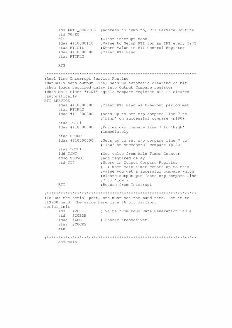
ldd #RTI_SERVICE ;Address to jump to, RTI Service Routine
std $07EC
cli ;Clear interupt mask
ldaa #%10000110 ;Value to Setup RTI for an INT every 32mS
staa RTICTL ;Store Value in RTI Control Register
ldaa #%10000000 ;Clear RTI Flag
staa RTIFLG
RTS
;****************************************************************
;Real Time Interrupt Service Routine
;Manually sets output line, sets up automatic clearing of bit
;then loads required delay into Output Compare register
;When Main timer "TCNT" equals compare register bit is cleared
;automatically
RTI_SERVICE
ldaa #%10000000 ;Clear RTI Flag as time-out period met
staa RTIFLG
ldaa #%11000000 ;Sets up to set o/p compare line 7 to
;'high' on successful compare (p190)
staa TCTL1
ldaa #%10000000 ;Forces o/p compare line 7 to 'high'
;immediately
staa CFORC
ldaa #%10000000 ;Sets up to set o/p compare line 7 to
;'low' on successful compare (p190)
staa TCTL1
ldd TCNT ;Get value from Main Timer Counter
addd SERVO1 ;add required delay
std TC7 ;Store in Output Compare Register
;--> When main timer counts up to this
;value you get a sucessful compare which
;clears output pin (sets o/p compare line
;7 to 'low')
RTI ;Return from Interrupt
;****************************************************************
;To use the serial port, one must set the baud rate. Set it to
;19200 baud. The value here is a 16 bit divisor.
serial_init
ldd #26 ; Value from Baud Rate Generation Table
std SC0BDH
ldaa #$0C ; Enable transceiver
staa SC0CR2
rts
;****************************************************************
end main
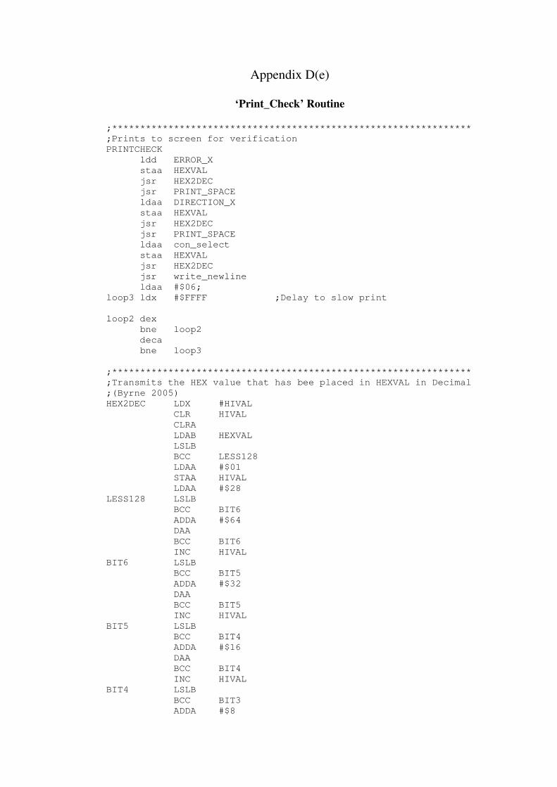
Appendix D(e)
‘Print_Check’ Routine
;****************************************************************
;Prints to screen for verification
PRINTCHECK
ldd ERROR_X
staa HEXVAL
jsr HEX2DEC
jsr PRINT_SPACE
ldaa DIRECTION_X
staa HEXVAL
jsr HEX2DEC
jsr PRINT_SPACE
ldaa con_select
staa HEXVAL
jsr HEX2DEC
jsr write_newline
ldaa #$06;
loop3 ldx #$FFFF ;Delay to slow print
loop2 dex
bne loop2
deca
bne loop3
;****************************************************************
;Transmits the HEX value that has bee placed in HEXVAL in Decimal
;(Byrne 2005)
HEX2DEC LDX #HIVAL
CLR HIVAL
CLRA
LDAB HEXVAL
LSLB
BCC LESS128
LDAA #$01
STAA HIVAL
LDAA #$28
LESS128 LSLB
BCC BIT6
ADDA #$64
DAA
BCC BIT6
INC HIVAL
BIT6 LSLB
BCC BIT5
ADDA #$32
DAA
BCC BIT5
INC HIVAL
BIT5 LSLB
BCC BIT4
ADDA #$16
DAA
BCC BIT4
INC HIVAL
BIT4 LSLB
BCC BIT3
ADDA #$8

DAA
BCC BIT3
INC HIVAL
BIT3 LSLB
BCC BIT2
ADDA #$4
DAA
BCC BIT2
INC HIVAL
BIT2 LSLB
BCC BIT1
ADDA #$2
DAA
BCC BIT1
INC HIVAL
BIT1 LSLB
BCC ALLDONE
ADDA #$1
DAA
BCC ALLDONE
INC HIVAL
ALLDONE LDAB #$30
ADDB HIVAL
STAB HIVAL
TAB
ANDA #%11110000
LSRA
LSRA
LSRA
LSRA
STAA 1,X
LDAA #$30
ADDA 1,X
STAA 1,X
ANDB #%00001111
STAB 2,X
LDAA #$30
ADDA 2,X
STAA 2,X
LDAA 0,X
JSR TXBYTE
LDAA 1,X
JSR TXBYTE
LDAA 2,X
JSR TXBYTE
RTS
;****************************************************************
;Transmit a character which is in A
txbyte
brclr SC0SR1, #$80 txbyte
staa SC0DRL
rts
;****************************************************************
;Send a carriage return and line feed to screen
write_newline
ldaa #$0D ;Load Carriage return ASCII
jsr txbyte
ldaa #$0A ;Load Line Feed ASCII
jsr txbyte

rts
;****************************************************************
;Print a space
PRINT_SPACE
ldaa #' '
jsr txbyte
rts
126
APPENDIX E
Technical Specifications of SensComp 6500 Series Ranging Module
(SensComp, 2004)

SensComp, Inc. 36704 Commerce Rd. Livonia, MI 48150 Telephone: (734) 953-4783 Fax: (734) 953-4518 www.senscomp.com
6500 Series Ranging Modules
Description
SensComp's Ranging Modules provide the drive electronics for SensComp Electrostatic Transducers Features: Accurate Sonar Ranging from 6 inches to 35 feet Drives a 50 kHz Electrostatic Transducer Without an Additional Interface Operates from a Single Power Supply Source Accurate Clock Output Provided for External Use Selective Echo Exclusion TTL Compatible Multiple Measurement Capability Integrated Transducer Cable Variable Gain Control Potentiometer
PID# 615078 -- 6500 Series Sonar Ranging Module PID# 615079 -- 6500 Series Enhanced Sonar Ranging Module;
Includes Pull-up Resistors and an Internal Oscillator for Repetitive Operation PID# 615080 -- 6500 Series Sonar Ranging Module ` Without the Connector
The 6500 Series is an economical sonar ranging module that can drive all SensCommodule, with a simple interface, is able to measure distances from 6 inches to 35 fethe reading over the entire range. This module has an external blanking input that allows selective echo exclusion for The module is able to differentiate echos from objects that are only three inches apavariable bandwidth amplifier minimizes noise and side-lobe detection in sonar applic The module has an accurate ceramic resonator controlled 420 kHz time base genertime base is provided for external use. The sonar transmit output is 16 cycles at a f The 6500 Series module operates over a DC power supply range from 4.5 volts to 6characterized for operation from 0° C to 40° C. For more information, visit our website: www.senscomp.com C
Features
Part No.
Specifications
p electrostatic transducers. This et. The typical accuracy is +/- 1% of
operation on a multiple-echo mode. rt. The digitally controlled gain, ations.
ator. An output based on the 420 kHz requency of 49.4 kHz.
.8 volts (5 volts nominal) and is
opyright © 2004 SensComp. Inc. 9/13/04

6500 Ranging Mod.-- page 2
Absolute Maximum Ratings over Operating Free-air temperature range Voltage from any pin to ground (see Note 1) ........................................................................................................ 7 VDC Voltage from any pin except XDCR to VCC (see Note 1) ....................................................................-7 VDC to 0.5 VDC Operating free-air temperature range..........................................................................................................0° C to 40° C Storage temperature range ......................................................................................................................-40° C to 85° C NOTE 1: The XDCR pin may be driven from -1 volt to 400 volts typical with respect to ground. Recommended Operating Conditions
MIN MAX UNIT Supply Voltage, Vcc 4.5 6.8 V High-level Input Voltage, VIH BLNK, BINH, INIT 2.1 V Low-level Input Voltage, VIL BLNK, BINH, INIT 0.6 V ECHO and OSC Output Voltage 6.8 V Delay Time, Power Up to INIT High 5 ms Recycle Period 80 ms Operating Free-air Temperature, TA 0 40 °C
Electrical Characteristics over Recommended Ranges of Supply Voltage and Operating Free-Air Temperature PARAMETER TEST COND. MIN TYP MAX UNIT Imput Current BLNK, BINH, INIT VI = 2.1 V 1 mA High-level Output Current, IOH ECHO, OSC VOH = 5.5V 100 µA Low-level Output Voltage, VOL, ECHO, OSC IO L= 1.6 mA 0.4 V Transducer Bias Voltage TA = 25° C 200 V Transducer Output Voltage (peak to peak) TA = 25° C 400 V No. of Cycles for XDCR Output to Reach 400V C = 500 pF 7 Internal Blanking Interval 2.38† ms XMIT Drive Signal Duration 1.1† ms Frequency During 16-pulse OSC output 49.4† kHz Transmit Period XMIT output 49.4† kHz Frequency After 16-pulse OSC output 93.3† kHz Transmit Period XMIT output 0 kHz Supply Current, Icc During transmit period 2000 mA
After transmit period 100 mA † These typical values apply for a 420 kHz ceramic resonator Operation With SensComp Electrostatic Transducers There are two basic modes of operation for the 6500 Series Sonar Ranging Modules: Single-echo mode and multiple-echo mode. The application of power (VCC), the application of the initiate (INIT) input, and the resulting transmit output, and the use of the Blanking Inhibit (BINH) input are basically the same for either mode of operation. After applying power (VCC) a minimum of 5 milliseconds must elapse before the INIT signal can be taken high. During this time, all internal circuitry is reset and the internal oscillator stabilizes. When INIT is raised to a high level, drive to the transducer (XDCR) output occurs. Sixteen pulses at 49.4 kHz with an amplitude of 0 volts to 400 volts peak to peak will excite the transducer as transmission occurs. At the end of the 16 transmitted pulses, a 200 VDC bias remains on the transducer (as recommended) for optimum receiving operation. In order to eliminate ringing of the transducer from being detected as a return signal, the Receive (REC) input of the ranging control IC is inhibited by internal blanking for 2.38 milliseconds after the initiate signal. If a reduced blanking time is desired, then the BINH input can be taken high to end the blanking of the Receive input any time prior to internal blanking. This may be desirable to detect objects closer than 1.33 feet (corresponding to 2.38 milliseconds) and may be done of transducer damping is sufficient so that ringing is not detected as a return signal. For more information, visit our website: www.senscomp.com Copyright © 2004 SensComp. Inc. 9/13/04

6500 Ranging Mod.-- page 3 In the single-echo mode of operation (Figure 1), all that must be done next is to wait for the return of the transmitted signal, traveling at approximately 0.9 milliseconds per foot out and back. The returning signal is amplified and appears as a high logic level echo output. The time between INIT going high and the Echo (ECHO) output going high is proportional to the distance of the target from the transducer. If desired, the cycle can now be repeated by returning INIT to a low logic level and then taking it h
igh when the next transmission is desired.
FIGURE 1: EXAMPLE OF A SINGLE-ECHO-MODE CYCLE WITHOUT BLANKING INPUT
there is more than one target and a single transmission detects multiple echos, then the cycle is slightly different (Figure
uring a cycle starting with INIT going high, the receiver amplifier gain is increased at discrete times (Figure 3) since the
st
For more information, visit our website: www.senscomp.com
If 2). After receiving the first return signal which causes the ECHO output to go high, the Blanking (BLNK) input must be taken high then back low to reset the ECHO output for the next return signal. The blanking signal must be at least 0.44 milliseconds in duration to account for all 16 returning pulses from the first target and allow for internal delay times. Thiscorresponds to the two targets being 3 inches apart. Dtransmitted signal is attenuated with distance. At approximately 38 milliseconds, the maximum gain is attained. Althoughgain can be increased by varying R1 (see Component Layout), there is a limit to which the gain can be increased for reliable module operation. This will vary from application to application. The modules are “kitted” prior to their final teduring manufacture. This is necessary because the desired gain distribution is much narrower than the module gain distribution if all were kitted with one value resistor. As kitted, these modules will perform satisfactorily in most applications. As a rule of thumb, the gain can be increased up to a factor of 4, if required, by increasing R1 correspondingly. Gain is directly proportional to R1.
Copyright © 2004 SensComp. Inc. 9/13/04

put/Output Schematic Notes:
E Enhanced SMT Ranging Module
In
he ECHO and OSC outputs are open collector NPN transistor outputs (Figure 4) requiring 4.7 Kohm pull-up resistors etween VCC and the output.
FIGURE 4: SCHEMATIC EQUIVALENT CIRCUITS OF BOARD INPUTS/OUTPUTS
Component Layouts
6500 SMT Ranging Module
PID#615078 PID#615079 For more information, visit our website: www.senscomp.com
Tb
6500
Copyright © 2004 SensComp. Inc. 9/13/04
6500 Ranging Mod.-- page 4

Schematic – 6500 SMT Ranging Module--PID#615078
For more information, visit our website: www.senscomp.com
6500 Ranging Mod.-- page 5
Copyright © 2004 SensComp. Inc. 9/13/04

Schematic – 6500E Enhanced SMT Ranging Module --PID#615079
or more information, visit our website: www.senscomp.comF Copyright © 2004 SensComp. Inc. 9/13/04
6500 Ranging Mod.-- page 6
Recommended