Automatic Generation of Bond Graph Models of Process Plants
Sebastian Beez
Helmut-Schmidt-University
Holstenhofweg 85
22043 Hamburg, Germany
Alexander Fay
Helmut-Schmidt-University
Holstenhofweg 85
22043 Hamburg, Germany
Nina Thornhill
Imperial College London
South Kensington Campus
London SW7 2AZ, UK
Abstract
This paper presents an application for the automatic
generation of Bond Graph models.
The basis for this automated creation is a modified
plant model in the XML-format according to the IEC
PAS 62424 (CAEX). The application developed in the
programming language C, extracts and converts the
information which is, then, stored in a model file
meeting the requirements and structure of the
modelling/ simulation-language Dymola. Bond Graphs
are used as the modelling technique since they do not
distinguish between different energy domains and,
therefore, combine several advantages against other
modelling techniques.
The developed application can be used for multiple
purposes such as simulations, visualizations and other
specific tasks that might emerge during the planning
and operation process of plants and other engineering
systems.
1. Introduction
Nowadays system models are used for various kinds
of simulations and research and the profit gained from
such models/ simulations is essential throughout the
different engineering steps of building, testing and
running all kinds of systems. The models therefore
need to act like their real counterparts in terms of
continuous behaviour. Especially if they represent a
chemical process that involves several media these
models should include the physics and laws of
hydrodynamics, reaction chemistry and heat- and
mass-transfer.
In general, creating models by hand is time-
consuming and, therefore, costs a lot of money. That is
why an automatic creation of such models from
existing plant data is a welcome and desirable
alternative. Object-oriented Computer Aided
Engineering tools offer the potential for such an
automatic creation.
Object-oriented representations of plants and
processes are becoming more available and are a
convenient way to store and exchange information
such as process diagrams between different
engineering domains. One way to do this is the
Computer Aided Engineering Exchange-format,
CAEX. Bond Graphs on the other hand are a modelling
method to describe the power flow within a system.
Bond Graphs allow the representation of hybrid
systems more easily than other modelling techniques
since they do not differentiate between mechanical,
thermal, hydraulic or other energy domain systems.
The work this paper is based on was carried out in
two projects. The main aim in the first project was to
provide an application which is able to automatically
generate Bond Graph models out of CAEX files. After
the first development stage of the application was
finished, the second project’s aim was to broaden the
abilities of the program and overcome limitations such
as elements lacking sensor- and actuator-interfaces and
multiple inflows and outflows. Furthermore, more
options for the user to influence the model had to be
implemented.
After this introduction into the topic, the second
chapter provides all the background knowledge needed
to understand the subsequent chapters. A brief
presentation of the tools and their common properties,
the preparatory work on the necessary data files and
the methods for the conversion are presented to the
reader. A validation chapter gives proof of the abilities
of the application and shows possible ways of using the
automatically generated models. A conclusive part
finalizes this paper by summarizing the achievements
and providing a future outlook.
2. CAEX and Bond Graphs
This section is to introduce the basis of this paper.
The Computer Aided Engineering Exchange-format
(CAEX), Bond Graphs, the modeling software Dymola
and their common properties will be presented in the
following sections.

2.1. CAEX
The CAEX format was developed by the Chair of
Process Control Engineering of RTWH Aachen and
ABB Research Centre. CAEX and other languages/
schemas are based on the Extensible Markup Language
(XML), which is a standard way to describe data. XML
was initially developed to share data across the internet
[9]. The CAEX schema functions as a vendor-
independent neutral data exchange format between
plant engineering tools. It was developed to reduce the
amount of costs and time during plant design. CAEX
represents the structural and functional behaviour of a
plant. Thus, CAEX models are meta-models which
describe elements in an abstract way and with an
arbitrary number of attributes. They contain the
information stored in Piping and Instrumentation
Diagrams (P&ID) as well as additional information.
The possibility to extend models is another important
feature. CAEX files are used during plant design thus
they enable different groups to add information and
pass the file on to the next group. CAEX methodology
provides this feature. The models can be extended and
completed anytime without a need to have a new
agreement of the structure.
Similar to XML, CAEX files have a schema, too. It
prescribes the structure of a CAEX file. At the
beginning of a document there is a declaration.
Thereafter the root node begins. Besides a header, a
CAEX root node has four major child notes. The
SystemHierarchy gives an overview of the whole
system and all the elements including all the links
between the elements. However, the SystemHierarchy
provides no further information about the elements.
The RoleClassLibrary lists all possible roles of
elements. It is comparable to the P&ID. Only a symbol
is used to describe a certain task, such as tank, valve,
pump and the like. The third major child node is the
SystemUnitClassLibrary. This library contains special
information about elements. It can present the internal
structure of an element as well as specifications and
operating parameters. This child node allows
integration of different libraries. For example,
companies can use it to supply a portfolio of their
products. The fourth child node is the
InterfaceClassLibrary, which describes different
interfaces and their characteristics.
Figure 1: Structure of a CAEX file (from Drath et al. (2005))
Figure 1 presented the CAEX schema used during
the projects.
Drath et al. (2005) provides further information on
the structure and the relations between these major
parts of the CAEX file.
2.2. Bond Graphs and Dymola
A Bond Graph is a modelling methodology that was
developed by Professor Henry M. Paynter. The main
idea is to model the power flow through a system
assuming energy conservation. This methodology has
several advantages. It is easier to model hybrid systems
since multi-energy domain models can be created
without a use for own models for every energy domain.
A second advantage is bi-directionality of the elements.
If elements produce any kind of effect that influences
upstream elements there is no need to model a
feedback loop. This effect will propagate backwards
through the upstream elements anyway.
The power flow is modelled using two variables,
effort, e, and flow, f, which yield power if multiplied.
Therefore they are called power-variables. Furthermore
there are momentum, p, and displacement, q, which
yield energy if multiplied. The relations between all
these variables are explained in more detail in Karnopp
et al. (1990) and Cellier (1991).
With the help of these variables a range of elements
was created. The developer was an electrical engineer,
thus, most of the elements that were used for creating
models have synonyms used in this particular area.
Basic components which appear in every system can be
modelled using the same variables and equations.
• Resistors, capacities, inductances
• Transformers and gyrators
• Effort and flow sources
• Parallel and series-junctions
appear in every system, energy domain independent.
Only the units are changing. That is why hybrid
systems are easier to handle with the Bond Graph
methodology. Further information related to Bond
Graphs can be found in Karnopp et al. (1990)and
Cellier (1991).
Dymola was the modelling/simulation software for
the projects. It is based on Modelica which is an
equation-based modelling language. Dymola enables
modelling via Drag&Drop and creates the Modelica
code behind the graphical models itself. There are
plenty of freeware libraries for Dymola for various
kinds of engineering areas, a Bond Graph library
amongst them. The Bond Graphs library includes a
well-equipped set of basic elements and some special
sub-libraries. Besides modelling, simulations can be
run with Dymola. The software includes several

solving algorithms and certain possibilities to influence
the simulation. Furthermore generated models can be
exported and used in other simulation environments
such as MatLab/Simulink.
For further information about Dymola itself or the
use of this software, see Fritzson (2004) or the Dymola
User Manual provided along with the program. The
following figure shows the Dymola window and a
model composed of Bond Graph elements.
Figure 2: Dymola User Interface with Bond Graph model
3. Generation methodology
3.1. Common properties
There are several similarities between CAEX files
and Bond Graph models in Dymola; especially
according to the structure. These similarities are most
helpful throughout an automatic conversion.
As mentioned in 2.1 CAEX the SystemHierarchy
lists all elements appearing in the system. This is
beneficial since a list of all the elements can be
generated and then worked off. Utilizing this, a
complete list of all the elements can be written into the
model file. The links between these elements, also
given in the SystemHierarchy, make up the second part
of the model file. Hence, they have to be transferred as
well. The SystemUnitClassLibrary contains special
information about each element. This is very
advantageous for specifying each element and
equipping it with its own properties. Since Dymola is
working with different libraries the RoleClassLibrary
in a CAEX file is a convenient place to store the
Dymola-library path of the corresponding element.
The CAEX requirements presented in the following
section presents how these structural similarities can be
used creating the CAEX file from which the model is
built.
3.2. CAEX requirements
The automatic generation of a Bond Graph model
demands information about all the elements. These
demands especially apply to the CAEX file that the
model is derived from. The following section points
out the conditions the CAEX file has to meet in order
for the conversion to function properly.
In more detail, the SystemHierarchy stores every
single element along with its individual references to
RoleClassLibrary and SystemUnitClassLibrary.
Furthermore the physical links to other elements are
listed. Since some elements have signal connections,
these links are stored in this section as well.
Following the reference in the SystemHierarchy, the
RoleClassLibrary provides the matching Bond Graph
element together with the path in the Bond Graph
library. That is due to the focus of this project, which
was not to scan this library for matching elements.
The SystemUnitClassLibrary has to provide the
parameters for the matching Bond Graph elements.
These parameters can either be abstract details like a
capacity according to a pressure if the component is a
basic Bond Graph element or, like in common CAEX
files, geometric details of the elements, such as height
and cross-section area if the model is one of the
components developed during the second project.
These requirements account for another important
aspect. The level of detail in the Dymola model is
determined by the level of detail provided in the CAEX
file. Thus, the more information about an element is
given in the CAEX file, the more detailed is the model
and the simulation result from this component.
3.3. Approach for the automatic generation
The generation methodology utilizes the common
properties in structure and the restriction put on the
content of the CAEX file.
The method of converting a CAEX file into a model
is divided into three parts. The first part comprises
collecting all the information from the CAEX file. The
fact that the SystemHierarchy contains all the elements
of the system makes it a convenient point to start with.
A list of all the elements is created first and then filled
with information about each component starting with
its name. The data about the links each element has to
the others is then taken from the CAEX file and added
to this list. Thereafter the references to its role and to
its specific and detailed information are tracked and
these information are written into the list as well. This
finalizes the first step of gathering all the information
and bundling it in a list. The following figures show a
CAEX file and its structure. They present an example
of two tanks and show how the information about these
tanks is structured.

Figure 3: SystemHierarchy of a CAEX file
The referenced RoleClasses and the
SystemUnitClasses are presented in the Figure 4.
Figure 4: RoleClass- and SystemUnitClass-Library of a CAEX file
After collecting all the information from the CAEX
file it needs to be adapted to the demands of the
modeling software. This means that the second step in
the developed methodology is reordering the gathered
information according to the structure of a single entry
in the model file and considering the overall structure
of the model file.
Finally, the third part of the generation methodology
is to write the model file. After a header and an
annotation necessary for the simulation in Dymola all
the components of the model are listed. After the
components and the keyword “equation” all the links
need to be written into the file. An end-section finished
the model file that looks like the following figure for
the example of the two tanks.
Figure 5: Model file in Dymola
4. Application of the methodology
The aim of this section is to explain how the
developed application utilizes the approach chosen for
the model generation. The three steps of the
methodology are maintained in general and will be
explained in more detail in the following lines.
The user determines the behaviour of the program.
Hence, the first part entails the user choosing a CAEX
file after having started the application. The second
part takes place without any user interaction. The data
from the chosen file is read and parsed into the
application. Every InternalElement in the
SystemHierarchy is allocated to an object. Not only is
the element name itself stored in this object, but also its
references and details. Finalizing the second part of the
generation methodology, the object is then added to an
elementList.
The Element-object and its attributes, where all the
data for a single component is stored in, is depicted in
the following figure. Thereafter the first step of the
generation methodology is summarized graphically.

Figure 6: Element-object and attributes
1. The User chooses a CAEX file
2. For each element in the file the following steps
are performed:
• Create an “Element”-object
• Save name from SystemHierarchy
• Add a number
• Save path in the Dymola library from the
referenced RoleClass
• Save specifications from the referenced
SystemUnitClass
• Save the connections from the
SystemHierarchy
• Add an x- and an y-position
• Add the “Element”-object to the elementList
Figure 7: Procedure of reading the CAEX file
The position-attributes are necessary for positioning
each component in the Dymola user interface. To
proceed with the generation of the model file further
user input is required. The user needs to provide a
model name and file path to store the model file to. In
addition, the user can manipulate the model by giving
parameters for the simulation. As an example, the user
can set the level of medium inside a tank to a certain
value at the beginning of the simulation. These
adjustments are added to the specification of the
pertaining element.
Step two is the biggest and most important step. It is
subdivided into two steps.
The first sub-step is reordering the attributes of each
element to meat the required structure for a single
component. In the case of Dymola as the modeling
language the single entry for a tank as shown in Figure
3 would then consist of the path in the Dymola library
(as given in the RoleClass), the name (as stated in the
SystemHierarchy) and the details (provided by the
SystemUnitClass). Every element from the first list and
its details is reordered like that and saved in a second
list. With respect to the overall structure of the Dymola
model only the reordered elements are included in this
second list, called entryList.
Before building the model file some of the elements
need further preparation. Since Bond Graphs are the
modelling technique, some elements such as resistors,
R, and capacitors, C, which are basic elements, need to
be attached to junctions in order to work. These
junctions and the bonds to connect elements and
junctions are also added to the entryList. The code for
the connections between the passive elements and the
bonds as well as between the bonds and the junctions is
stored in the third list, called connectList.
The second sub-step is to link all the elements
according to the information gained from the CAEX
file. The information about the links between the
elements is taken from the first list, reordered and
written into the connectList. The following figure
summarizes step two.
1. For each object in the elementList the following
steps are performed:
• The details are reordered and added to the
entryList
• If necessary, bonds and junctions are added
to the entryList
• Connections between the component, bond
and junction are added to the connectList
• Connections between the components are
written into the connectList
Figure 8: Preparing and linking the elements
Finally, the model file itself is created. This starts
with opening a new file and writing the header in. It
consists of the keyword model, the name (provided by
the user via the Graphical User Interface) and some
annotations for Dymola to compile the model. After
the header section, all the elements are listed. After
completing the entryList in the last step, each entry is
written into the model file. Then the keyword equation
followed by the content of the connectList is added to
the model file. Finalizing this step, the keyword end
and the model name are written to the model file.
Thereafter the file is saved, shut and looks like Figure
5: Model file in Dymola. Figure 9 summarizes the final
part of the model generation if Dymola is the
modelling language.
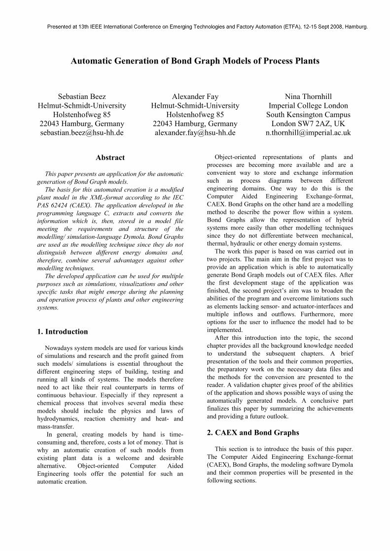
1. Open a model file to write in
2. Write header-section
3. Write all entries into the file
4. Add the keyword “equation”
5. Write all connections into the file
6. Write end-section
Figure 9: Writing the model file
Confirmation dialogs inform the user about the
CAEX file having been read in and the model file
having been created successfully. For detailed
information about the generation methodology see
Beez (2007). The following figure summarizes the
methodology graphically.
Figure 10: Generation methodology
5. Validation example
After an application is developed it needs to be
tested and validated. Within this section the application
has to prove that it can handle bondgraphic elements
and that the developed methodology of creating models
automatically functions. The aim is a model that can be
compiled without errors and simulations can be run
with it. In this section the pumped-storage power
station build in Goldisthal, Germany, stands as the
system the model is build from. Secondly, this section
is to show that using these models can be useful for
various purposes such as prediction, testing and
verifying a controller-setup and many more.
Due to the ability of pumped-storage plants to
produce a considerable amount of power within
minutes and, therefore, giving the opportunity to react
to load changes in the electricity network they are a
welcome option. They are furthermore a cost-efficient
way of storing energy during times of low demand.
That is why models of such system might be welcome
for prediction or to test and verify controllers.
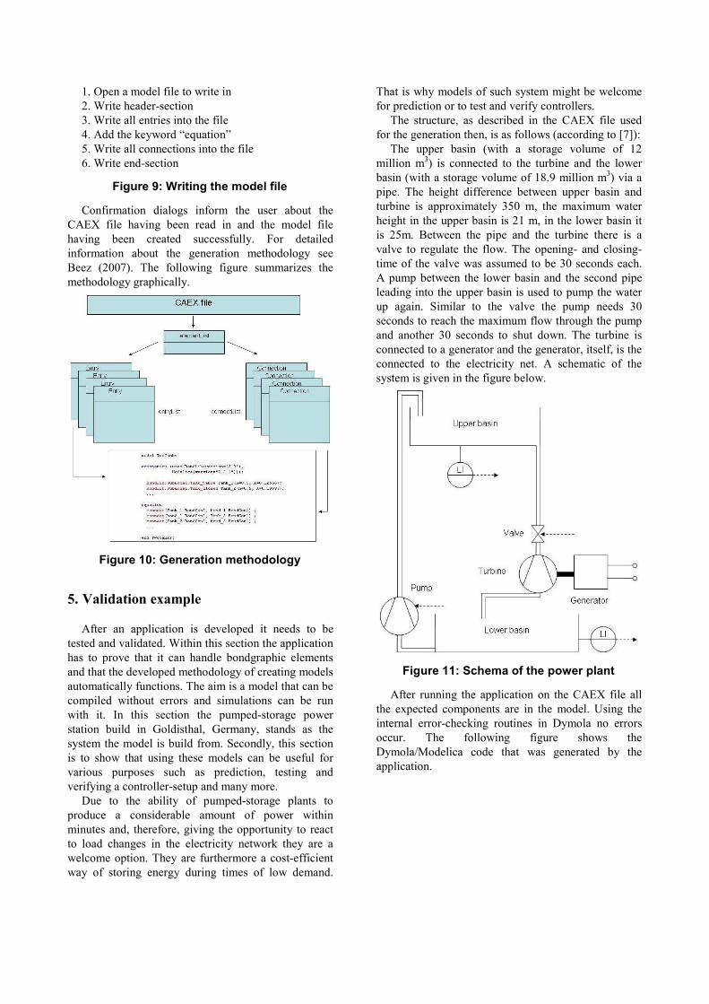
The structure, as described in the CAEX file used
for the generation then, is as follows (according to [7]):
The upper basin (with a storage volume of 12
million m3) is connected to the turbine and the lower
basin (with a storage volume of 18.9 million m3) via a
pipe. The height difference between upper basin and
turbine is approximately 350 m, the maximum water
height in the upper basin is 21 m, in the lower basin it
is 25m. Between the pipe and the turbine there is a
valve to regulate the flow. The opening- and closing-
time of the valve was assumed to be 30 seconds each.
A pump between the lower basin and the second pipe
leading into the upper basin is used to pump the water
up again. Similar to the valve the pump needs 30
seconds to reach the maximum flow through the pump
and another 30 seconds to shut down. The turbine is
connected to a generator and the generator, itself, is the
connected to the electricity net. A schematic of the
system is given in the figure below.
Figure 11: Schema of the power plant
After running the application on the CAEX file all
the expected components are in the model. Using the
internal error-checking routines in Dymola no errors
occur. The following figure shows the
Dymola/Modelica code that was generated by the
application.

Figure 12: Generated model code
After making use of the possibility to add a start-
value for the height of water in the upper basin during
the conversion and running a simulation in Dymola,
the following figure shows a curve for the power
output of the plant into the net in case the valve is
completely opened.
Figure 13: Simulation result for the generator
As expected, the power output slowly decreases
from 1.08 GW in the beginning to 1.07 GW over a
period of 7.5 hours. This is due to the lower water level
in the upper basin in the end. This is another proof for
the accuracy of the models. The time the upper basin
needs to run dry is approximately the same as stated in
[7].
The fact that no errors occur and the simulation is
running as expected gives proof for the application’s
ability to handle the automatically generated.
Replacing the simple controller used in this simulation
with a controller that represents a real supply and
demand-curve as shown in [8], the model can be used
for various purposes as mentioned above.
6. Conclusion
The resulting program has proven able to create
Bond Graph models out of CAEX files which match
the given restrictions. Checking these models with the
Dymola check-routine has showed that the models
have no errors and that simulations can be run with
them. Another important aspect is that the program
code was written with an eye on future changes and
further developments and, therefore, is maintained
flexible.
As already mentioned possible uses for the
application are various. The models generated could be
used for testing and verifying controller set-ups, they
could be implemented as simple models of systems
used for prediction inside a Model Predictive
Controller (MPC) or for simulations on systems in
general.
On a long-term basis the models could be utilized
for simulations on fault detection. However, this would
require much more precision than and, thus, the
development of precise component-models.
Furthermore heat and multi-media models would have
to be included. Another usage on a long-term basis
might be visualizing the power flow within a system
and, based on that, an optimization of the process itself
or the architecture of a plant or system in general. For
the purpose of visualizing the power flow the use of
Power Bonds as explained in Beez (2008) can be most
helpful.
References
[1] W3C 2007, World Wide Web Consortium, viewed 25
October, 2007, <www.w3.org>.
[2] R. Drath & M. Fedai, “CAEX – a neutral data
exchange format for engineering data”, atp –
Automatisierungstechnische Praxis, Vol. 3, pp. 50–62,
2005.

[3] D. C. Karnopp & D. L. Margolis & R. C. Rosenberg,
System Dynamics: A Unified Approach, 2nd edn, John
Wiley & Sons, 1990.
[4] F. E. Cellier, Continuous System Modeling, Springer-
Verlag, 1991.
[5] P. Fritzson, Principles of Object-Oriented Modeling
and Simulation with Modelica 2.1, John Wiley & Sons,
2004.
[6] S. Beez, Automatic generation of Bond Graph models
out of CAEX: Requirements, possibilities and
limitations, available via: Prof. Alexander Fay
([email protected]), Institut fuer
Automatisierungstechnik, Helmut-Schmidt-University,
Hamburg, 2007.
[7] Pumped Storage Power Plant Goldisthal Germany,
Lahmeyer International, viewed 01 March, 2008,
<http://www.lahmeyer.de/e/units/ge/ps_ge1_e_200002
_goldisthal_2004_03.pdf>
[8] Wikipedia – The Free Encyclopedia 2008, Wikipedia
Foundation, Inc., St. Petersburg, Florida, viewed 01
March, 2008, <http://de.wikipedia.org/wiki
/Bild:Pumpspeicherkraftwerk.png>.
[9] S. Beez, Automatic Generation of Bond Graph Models
of Process Plants, available via: Prof. Alexander Fay
([email protected]), Institut fuer
Automatisierungstechnik, Helmut-Schmidt-University,
Hamburg, 2008.
Recommended