#1
Automated Theorem Proving:Satisfiability Modulo Theories

#2
One-Slide Summary• An automated theorem prover is an algorithm that determines
whether a mathematical or logical proposition is valid (satisfiable).
• A theory is a set of sentences with a deductive system that can determine satisfiability.
• A satisfiability modulo theories (SMT) instance is a proposition that can include logical connectives, equality, and terms from various theories.
• The theory of equality can be decided via congruence closure using union-find.
• DPLL(T) is an SMT algorithm that uses a modified DPLL SAT solver, a well-defined interface for Theories, and a mapping between propositional variables and Theory literals.
• We can use logical rules of inference to encode proofs. Proof checking is like type checking.

#3
Combined Motivation
• We have seen:– How to handle (A || !B) => (!A || C)
• Satisfied by {A, C}, for example
• Arbitrary boolean expressions of boolean variables
– How to handle (x + y <= 5) && (2x >= 10)• Satisfied by {x = 5, y = 0}, for example
• Conjunctions of linear inequalities of real variables
• But what about:– (strlen(x) + y <= 5) => (strcat(x,x) != “abba”)
• Satisfied by {x = “abc”, y = 3}, for example

#4
High-Level Approach
• Beyond basic logic, we want to reason about– Strings: strlen(x), regexp_match(x, “[0-9]+”), ...
– Equality: a = b => f(a) = f(b), ...
– Linear Arithmetic: 2x+3y <= 10, …
– Bitvectors: (x >> 2) | y == 0xff, …
– Lists: head(cons(p,q)) = p
• All at the same time!• We will handle each domain separately (as a
theory) and then combine them all together using DPLL and SAT as the “glue”.

#5
Overall Plan
• Theory Introduction• Theory of Equality
– Congruence Closure
• The DPLL(T) solver for SMT– Formal Theory Interface
– Changes to DPLL
• Proof and Proof Checking

#6
I Have a Theory: It Could Be Bunnies
• In general, a theory is a set of sentences (syntax) with a deductive system that can determine satisfiability (semantics).
• Usually, the set of sentences is formally defined by a grammar of terms over atoms. The satisfying assignment (or model, or interpretation) maps literals (terms or negated terms) to booleans.
• We will consider theories that reason about conjunctions of literals.

#7
Theory of Linear Inequalities
• Given a finite set of variables V and a finite set of real-valued constants C
• Term ::= C1V
1 + … + C
nV
n <= C
n+1
• Conjunctions of terms can be decided via the Simplex method
#8
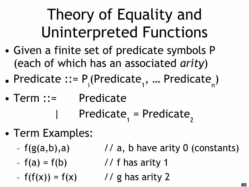
Theory of Equality and Uninterpreted Functions
• Given a finite set of predicate symbols P (each of which has an associated arity)
• Predicate ::= Pi(Predicate
1, … Predicate
n)
• Term ::= Predicate | Predicate
1 = Predicate
2
• Term Examples:– f(g(a,b),a) // a, b have arity 0 (constants)
– f(a) = f(b) // f has arity 1
– f(f(x)) = f(x) // g has arity 2

#9
Theory of Equality Definition
• Theory of equality with uninterpreted functions
• Symbols: =, , f, g, …• Axiomatically defined (A,B,C are Predicates):
• Reflexive, Symmetric, Transitive, Definition of A Function (Extensionality)
A=A A=B
B=A
A=C
A=B B=C
f(A) = f(B)
A=B

#10
Solving Equality
• Consider this conjunction of literals in the theory of equality:
g(g(g(x)))=x && g(g(g(g(g(x)))))=x && g(x)x• Is it satisfiable?
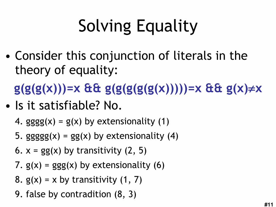
#11
Solving Equality
• Consider this conjunction of literals in the theory of equality:
g(g(g(x)))=x && g(g(g(g(g(x)))))=x && g(x)x• Is it satisfiable? No.
4. gggg(x) = g(x) by extensionality (1)
5. ggggg(x) = gg(x) by extensionality (4)
6. x = gg(x) by transitivity (2, 5)
7. g(x) = ggg(x) by extensionality (6)
8. g(x) = x by transitivity (1, 7)
9. false by contradition (8, 3)
#12
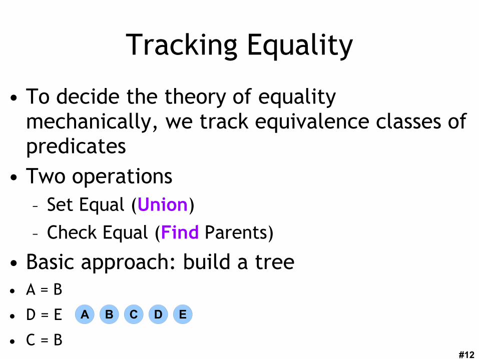
Tracking Equality
• To decide the theory of equality mechanically, we track equivalence classes of predicates
• Two operations– Set Equal (Union)
– Check Equal (Find Parents)
• Basic approach: build a tree• A = B
• D = E
• C = B
A B C D E

#13
Tracking Equality
• To decide the theory of equality mechanically, we track equivalence classes of predicates
• Two operations– Set Equal (Union)
– Check Equal (Find Parents)
• Basic approach: build a tree• A = B
• D = E
• C = B
A B C D E A
B
C D E
#14
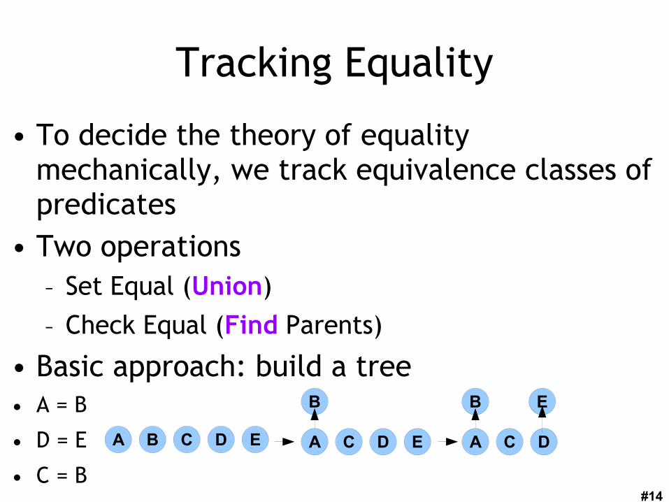
Tracking Equality
• To decide the theory of equality mechanically, we track equivalence classes of predicates
• Two operations– Set Equal (Union)
– Check Equal (Find Parents)
• Basic approach: build a tree• A = B
• D = E
• C = B
A B C D E A
B
C D E A
B
C D
E

#15
Tracking Equality
• To decide the theory of equality mechanically, we track equivalence classes of predicates
• Two operations– Set Equal (Union)
– Check Equal (Find Parents)
• Basic approach: build a tree• A = B
• D = E
• C = B
A B C D E A
B
C D E A
B
C D
E
A
B
C D
E

#16
Analogy: Raindrops Merging

#17
Two Optimizationslet union x y =
let x_root, y_root = find x, find y in
if x_root = y_root then return ()
if x_root.depth < y_root.depth
x_root.parent := y_root
else if y_root.depth < x_root.depth
y_root.parent := x_root
else
y_root.parent := x_root
x_root.depth := x_root.depth + 1
Keep trees short!Add smaller treeto bigger tree.
Only increases totalDepth if depths
Were equal!
#18
Analogy:Forwarding vs. Change of Address

#19
Two Optimizations
let rec find x = if x.parent != x then x.parent := find(x.parent) return x.parent
• This is called path compression.
A
B
CD
Efind A
A
BC
D
E

#20
Union-Find Analysis
• This is known as a “union-find” or “disjoint union” or “congruence closure” data structure.
• With the two optimizations, the amortized running time is O( inverse_ackermann (N) )– inverse_ackermann(N) <= 5 for N <= 2^2^65536
• So the amortized time is effectively constant.• “Fast Decision Procedures based on
Congruence Closure”, Nelson & Oppen, 1980

#21
Equality Decision ProcedureIdea
• Idea: start with the graph based on the conjunction of literals given– f(x) = g(z) && x = y
&& f(y) != g(z)
• There is a unique minimal graph corresponding to the congruence closure of the quality relation (i.e., if you know a=b and b=c, add the a=c edge).
• Compute that graph via union-find, but when you learn a=b, also add f(a)=f(b).
xy z
f gf

#22
Equality Decision ProcedureIntermediate Steps
let rec merge u v = (* add “u == v” *)
if find(u) = find(v) then return ()
let p_u = preds_of (eq_class_of u) in
let p_v = preds_of (eq_class_of v) in
union u v ;
for each (x,y) in p_u, p_v do (* u=v => f(u) = f(v) *)
if find x <> find y && congruent x y then
merge x y
let congruent x y =
return (out_degree x = out_degree y)
&& forall i. find x.child[i] = find y.child[i]

#23
Equality Decision Procedure
• Input:
– t1 = t'
1 && t
2 = t'
2 && … t
p = t'
p
– r1 != r'
1 && … r
2 != r'
2 && … r
q != r'
q
• Construct the graph where the vertices correspond to the terms and the edges correspond to function application
• for i = 1 … p: merge ti t'
i
• for i= 1 … q: if find ri = find r'
i then FALSE
• TRUE

#24
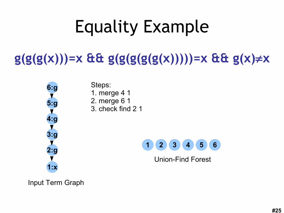
Equality Example
g(g(g(x)))=x && g(g(g(g(g(x)))))=x && g(x)x
1:x
2:g
3:g
4:g
5:g
6:g
1 2 3 4 5 6
Input Term Graph
Union-Find Forest
#25
Equality Example
g(g(g(x)))=x && g(g(g(g(g(x)))))=x && g(x)x
1:x
2:g
3:g
4:g
5:g
6:g
1 2 3 4 5 6
Input Term Graph
Union-Find Forest
Steps:1. merge 4 12. merge 6 13. check find 2 1
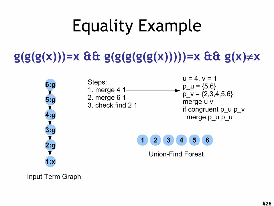
#26
Equality Example
g(g(g(x)))=x && g(g(g(g(g(x)))))=x && g(x)x
1:x
2:g
3:g
4:g
5:g
6:g
1 2 3 4 5 6
Input Term Graph
Union-Find Forest
Steps:1. merge 4 12. merge 6 13. check find 2 1
u = 4, v = 1p_u = {5,6}p_v = {2,3,4,5,6}merge u vif congruent p_u p_v merge p_u p_u

#27
Equality Example
g(g(g(x)))=x && g(g(g(g(g(x)))))=x && g(x)x
1:x
2:g
3:g
4:g
5:g
6:g
1 2 3
4
5 6
Input Term Graph
Union-Find Forest
Steps:1. merge 4 12. merge 6 13. check find 2 1
u = 4, v = 1p_u = {5,6}p_v = {2,3,4,5,6}merge u vif congruent p_u p_v merge p_u p_u

#28
Equality Example
g(g(g(x)))=x && g(g(g(g(g(x)))))=x && g(x)x
1:x
2:g
3:g
4:g
5:g
6:g
1 2 3
4
5 6
Input Term Graph
Union-Find Forest
Steps:1. merge 4 12. merge 6 13. check find 2 1
u = 4, v = 1p_u = {5,6}p_v = {2,3,4,5,6}merge u vif congruent 5 2 // 5 != 2, 5.child = 2.child merge 5 2

#29
Equality Example
g(g(g(x)))=x && g(g(g(g(g(x)))))=x && g(x)x
1:x
2:g
3:g
4:g
5:g
6:g
1 2 3
4 5
6
Input Term Graph
Union-Find Forest
Steps:1. merge 4 12. merge 6 13. check find 2 1
u = 4, v = 1p_u = {5,6}p_v = {2,3,4,5,6}merge u vif congruent 5 2 // 5 != 2, 5.child = 2.child merge 5 2

#30
Equality Example
g(g(g(x)))=x && g(g(g(g(g(x)))))=x && g(x)x
1:x
2:g
3:g
4:g
5:g
6:g
1 2 3
4 5
6
Input Term Graph
Union-Find Forest
Steps:1. merge 4 12. merge 6 13. check find 2 1
u = 4, v = 1p_u = {5,6}p_v = {2,3,4,5,6}merge u vif congruent 6 3 // 6 != 3, 6.child = 3.child merge 6 3
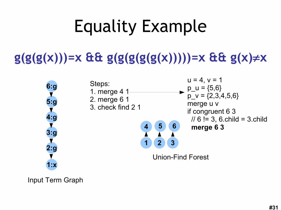
#31
Equality Example
g(g(g(x)))=x && g(g(g(g(g(x)))))=x && g(x)x
1:x
2:g
3:g
4:g
5:g
6:g
1 2 3
4 5 6
Input Term Graph
Union-Find Forest
Steps:1. merge 4 12. merge 6 13. check find 2 1
u = 4, v = 1p_u = {5,6}p_v = {2,3,4,5,6}merge u vif congruent 6 3 // 6 != 3, 6.child = 3.child merge 6 3

#32
Equality Example
g(g(g(x)))=x && g(g(g(g(g(x)))))=x && g(x)x
1:x
2:g
3:g
4:g
5:g
6:g
1 2 3
4 5 6
Input Term Graph
Union-Find Forest
Steps:1. merge 4 12. merge 6 13. check find 2 1
u = 6, v = 1p_u = {4,5,6}p_v = {1,2,3,4,5,6}merge u vif congruent p_u p_v merge p_u p_v
#33
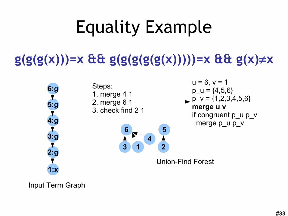
Equality Example
g(g(g(x)))=x && g(g(g(g(g(x)))))=x && g(x)x
1:x
2:g
3:g
4:g
5:g
6:g
1 234
56
Input Term Graph
Union-Find Forest
Steps:1. merge 4 12. merge 6 13. check find 2 1
u = 6, v = 1p_u = {4,5,6}p_v = {1,2,3,4,5,6}merge u vif congruent p_u p_v merge p_u p_v

#34
Equality Example
g(g(g(x)))=x && g(g(g(g(g(x)))))=x && g(x)x
1:x
2:g
3:g
4:g
5:g
6:g
1 234
56
Input Term Graph
Union-Find Forest
Steps:1. merge 4 12. merge 6 13. check find 2 1
u = 6, v = 1p_u = {4,5,6}p_v = {1,2,3,4,5,6}merge u vif congruent 4 2 // 4 != 2, 4.child = 2.child merge 4 2

#35
Equality Example
g(g(g(x)))=x && g(g(g(g(g(x)))))=x && g(x)x
1:x
2:g
3:g
4:g
5:g
6:g
1 234
56
Input Term Graph
Union-Find Forest
Steps:1. merge 4 12. merge 6 13. check find 2 1
u = 6, v = 1p_u = {4,5,6}p_v = {1,2,3,4,5,6}merge u vif congruent 4 2 // 4 != 2, 4.child = 2.child merge 4 2

#36
Equality Example
g(g(g(x)))=x && g(g(g(g(g(x)))))=x && g(x)x
1:x
2:g
3:g
4:g
5:g
6:g
12 34
56
Input Term Graph
Union-Find Forest
Steps:1. merge 4 12. merge 6 13. check find 2 1
u = 6, v = 1p_u = {4,5,6}p_v = {1,2,3,4,5,6}merge u vif congruent 4 2 // 4 != 2, 4.child = 2.child merge 4 2

#37
Equality Example
g(g(g(x)))=x && g(g(g(g(g(x)))))=x && g(x)x
1:x
2:g
3:g
4:g
5:g
6:g
12 34
56
Input Term Graph
Union-Find Forest
Steps:1. merge 4 12. merge 6 13. check find 2 1
they are equivalent: return false!

#38
Q. Computer Science
• This algorithmic strategy is applicable to decomposable problems that exhibit the optimal substructure property (in which the optimal solution to a problem P can be constructed from the optimal solutions to its overlapping subproblems). The term was coined in the 1940's by Richard Bellman. Problems as diverse as “shortest path”, “sequence alignment” and “CFG parsing” use this approach.

#39
Analogy: (NP-Hard) Reduction
Input Instance
InputConversion(to matchinterface)
Black-BoxOracle
OutputConversion
FinalAnswer

#40
Theory Interface• Initialize(universe : Literal Set)• SetTrue(l : Literal) : Literal Set
– Raise exception if l is inconsistent. Otherwise, add l to set of known facts. Return newly implied set of true facts (e.g., “a=c” after “a=b” and “b=c”)
• Backtrack(n : Nat)– Forget last n facts from “SetTrue”.
• IsDefinitelyTrue(l : Literal) : Bool• Explanation(l : Literal) : Literal Set
– If l is true, return a model (proof) of it.

#41
Satisfiability Modulo Theories
• A satisfiability modulo theories (SMT) solver operates on propositions involving both logical terms and terms from theories.
• Modern SMT solvers can use any theory that satisfies the Theory Interface shown before.
• Replace Theory clauses with special propositional variables.
• Use a pure SAT solver. If the solution involves some theory clauses, ask the Theory if they can all be true. If not, add constraints and restart.

#42
SMT Basic Idea• Given a query like
– (x > 5) && (p || (x < 4)) && !p
• Note that almost everything can be handled by SAT:– (x > 5) && (p || (x < 4)) && !p
– Only the highlighted parts require a Theory.
• So ask SAT to consider:– T1 && (p || T2) && !p
• And then whenever SAT gives a model, ask the theories if that model makes sense.
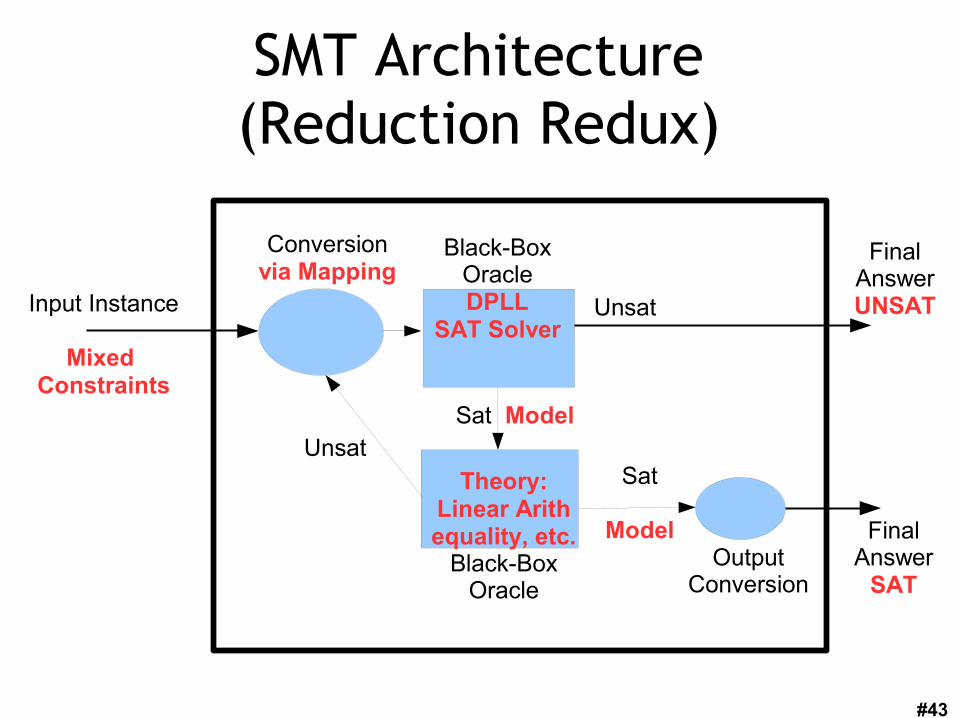
#43
SMT Architecture(Reduction Redux)
Input Instance
Mixed Constraints
Conversionvia Mapping
Theory:Linear Arithequality, etc.
Black-BoxOracle
OutputConversion
FinalAnswer
SAT
Black-BoxOracleDPLL
SAT Solver
UnsatSat
Model
Sat Model
Unsat
FinalAnswerUNSAT

#44
SMT Example
• Input: (x > 5) && (p || (x < 4)) && !p• Rewrite: T1 && (p || T2) && !p
– T1 = “x > 5” // mapping
– T2 = “x < 4”
• SAT solver returns {T1, T2, !p}• Ask Theory about T2 && T2
– Theory Query: (x > 5) && (x < 4)
– Theory Result: Unsatisfiable!
• T1 && (p || T2) && !p && !(T1 && T2)
#45
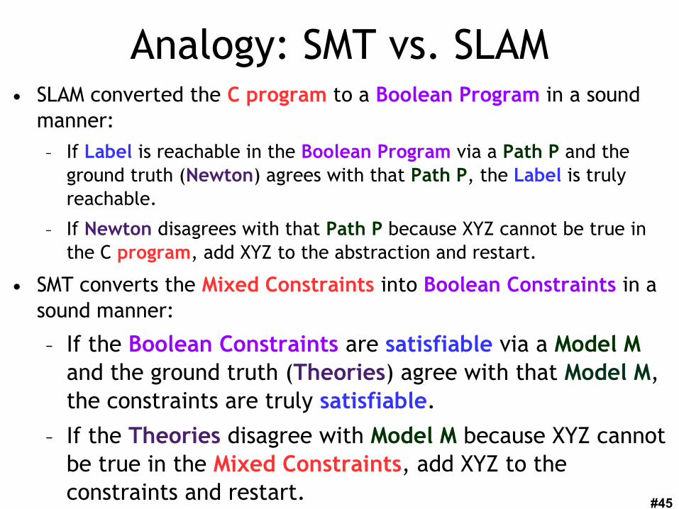
Analogy: SMT vs. SLAM• SLAM converted the C program to a Boolean Program in a sound
manner:
– If Label is reachable in the Boolean Program via a Path P and the ground truth (Newton) agrees with that Path P, the Label is truly reachable.
– If Newton disagrees with that Path P because XYZ cannot be true in the C program, add XYZ to the abstraction and restart.
• SMT converts the Mixed Constraints into Boolean Constraints in a sound manner:
– If the Boolean Constraints are satisfiable via a Model M and the ground truth (Theories) agree with that Model M, the constraints are truly satisfiable.
– If the Theories disagree with Model M because XYZ cannot be true in the Mixed Constraints, add XYZ to the constraints and restart.
#46
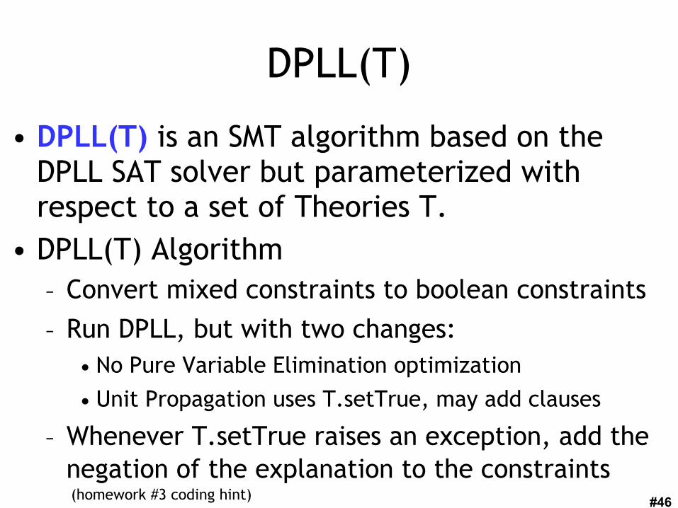
DPLL(T)
• DPLL(T) is an SMT algorithm based on the DPLL SAT solver but parameterized with respect to a set of Theories T.
• DPLL(T) Algorithm– Convert mixed constraints to boolean constraints
– Run DPLL, but with two changes:• No Pure Variable Elimination optimization
• Unit Propagation uses T.setTrue, may add clauses
– Whenever T.setTrue raises an exception, add the negation of the explanation to the constraints (homework #3 coding hint)
#47
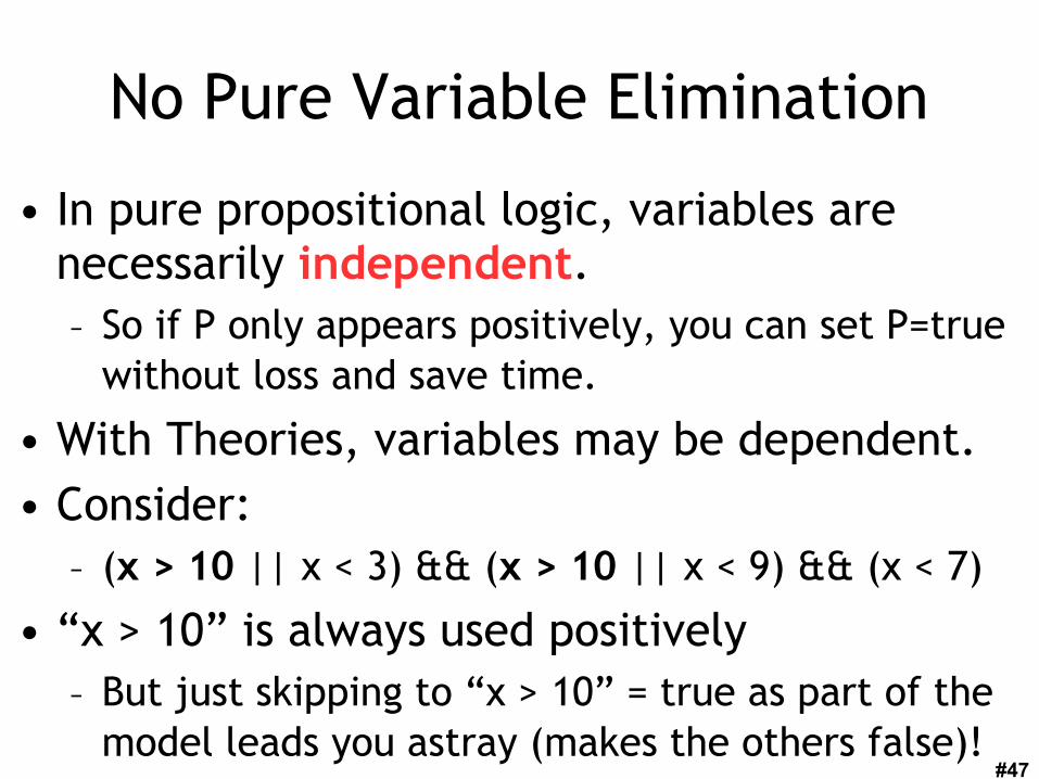
No Pure Variable Elimination
• In pure propositional logic, variables are necessarily independent.– So if P only appears positively, you can set P=true
without loss and save time.
• With Theories, variables may be dependent.• Consider:
– (x > 10 || x < 3) && (x > 10 || x < 9) && (x < 7)
• “x > 10” is always used positively– But just skipping to “x > 10” = true as part of the
model leads you astray (makes the others false)!
#48
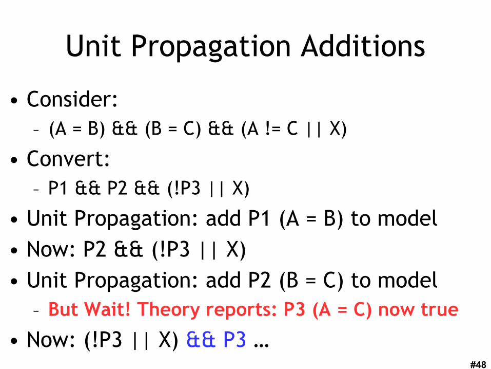
Unit Propagation Additions
• Consider:– (A = B) && (B = C) && (A != C || X)
• Convert:– P1 && P2 && (!P3 || X)
• Unit Propagation: add P1 (A = B) to model• Now: P2 && (!P3 || X)• Unit Propagation: add P2 (B = C) to model
– But Wait! Theory reports: P3 (A = C) now true
• Now: (!P3 || X) && P3 …

#49
DPLL(T) Example
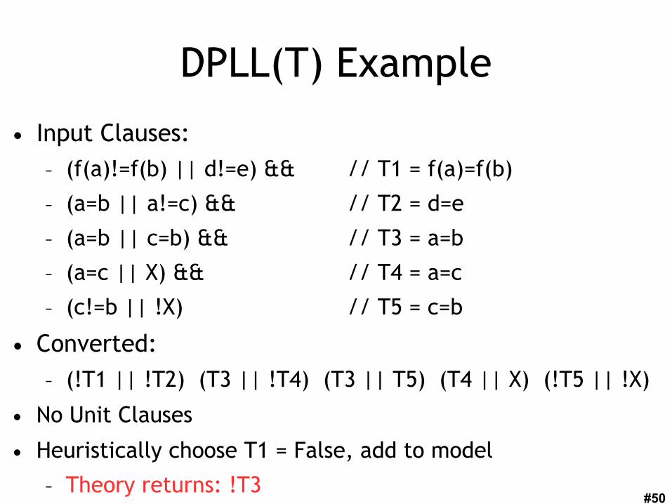
• Input Clauses:
– (f(a)!=f(b) || d!=e) && // T1 = f(a)=f(b)
– (a=b || a!=c) && // T2 = d=e
– (a=b || c=b) && // T3 = a=b
– (a=c || X) && // T4 = a=c
– (c!=b || !X) // T5 = c=b
• Converted:
– (!T1 || !T2) (T3 || !T4) (T3 || T5) (T4 || X) (!T5 || !X)
• No Unit Clauses
• Heuristically choose T1 = False, add to model
#50
DPLL(T) Example
• Input Clauses:
– (f(a)!=f(b) || d!=e) && // T1 = f(a)=f(b)
– (a=b || a!=c) && // T2 = d=e
– (a=b || c=b) && // T3 = a=b
– (a=c || X) && // T4 = a=c
– (c!=b || !X) // T5 = c=b
• Converted:
– (!T1 || !T2) (T3 || !T4) (T3 || T5) (T4 || X) (!T5 || !X)
• No Unit Clauses
• Heuristically choose T1 = False, add to model
– Theory returns: !T3

#51
DPLL(T) Example
• Input Clauses:
– (f(a)!=f(b) || d!=e) && // T1 = f(a)=f(b)
– (a=b || a!=c) && // T2 = d=e
– (a=b || c=b) && // T3 = a=b
– (a=c || X) && // T4 = a=c
– (c!=b || !X) // T5 = c=b
• Converted:
– (!T4) (T5) (T4 || X) (!T5 || !X)
• Model: !T1, !T3

#52
DPLL(T) Example
• Input Clauses:
– (f(a)!=f(b) || d!=e) && // T1 = f(a)=f(b)
– (a=b || a!=c) && // T2 = d=e
– (a=b || c=b) && // T3 = a=b
– (a=c || X) && // T4 = a=c
– (c!=b || !X) // T5 = c=b
• Converted:
– (!T4) (T5) (T4 || X) (!T5 || !X)
• Model: !T1, !T3
• Unit Clauses: !T4, !T5, add to model

#53
DPLL(T) Example
• Input Clauses:
– (f(a)!=f(b) || d!=e) && // T1 = f(a)=f(b)
– (a=b || a!=c) && // T2 = d=e
– (a=b || c=b) && // T3 = a=b
– (a=c || X) && // T4 = a=c
– (c!=b || !X) // T5 = c=b
• Converted:
– (X) (!X)
• Model: !T1, !T3, !T4, !T5
• Unit Clause: (X), add to model
#54
DPLL(T) Example
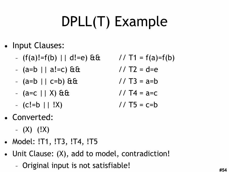
• Input Clauses:
– (f(a)!=f(b) || d!=e) && // T1 = f(a)=f(b)
– (a=b || a!=c) && // T2 = d=e
– (a=b || c=b) && // T3 = a=b
– (a=c || X) && // T4 = a=c
– (c!=b || !X) // T5 = c=b
• Converted:
– (X) (!X)
• Model: !T1, !T3, !T4, !T5
• Unit Clause: (X), add to model, contradiction!
– Original input is not satisfiable!
#55
DPLL(T) Conclusion
• DPLL(T) is widely used as a basis for modern SMT solving.– It is typically much faster than eagerly encoding
all of the variables into bits (e.g., 32-bit integer: 32 boolean variables). It is general in that it allows many types of theories.
• For example, Microsoft's popular and powerful Z3 automated theorem prover handles many theories, but uses DPLL(T) + Simplex for linear inequalities.
– “A Fast Linear-Arithmetic Solver for DPLL(T)”, 2006

#56
Proofs“Checking proofs ain’t like dustin’ crops, boy!”

#57
Proof Generation
• We want our theorem prover to emit proofs– No need to trust the prover
– Can find bugs in the prover
– Can be used for proof-carrying code
– Can be used to extract invariants
– Can be used to extract models (e.g., in SLAM)
• Implements the soundness argument– On every run, a soundness proof is constructed

#58
Proof Representation
• Proofs are trees– Leaves are hypotheses/axioms– Internal nodes are inference rules
• Axiom: “true introduction”– Constant: truei : pf– pf is the type of proofs
• Inference: “conjunction introduction”– Constant: andi : pf pf pf→ →
• Inference: “conjunction elimination”– Constant: andel : pf → pf
• Problem:– “andel truei : pf” but does not represent a valid proof– Need a powerful system that checks content
|- true
|- A
|- A && B
|- A &&B
|- A |- B
truei
andi
andel
#59
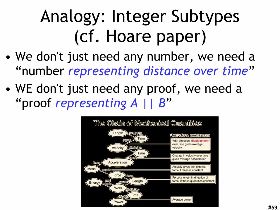
Analogy: Integer Subtypes(cf. Hoare paper)
• We don't just need any number, we need a “number representing distance over time”
• WE don't just need any proof, we need a “proof representing A || B”
#60
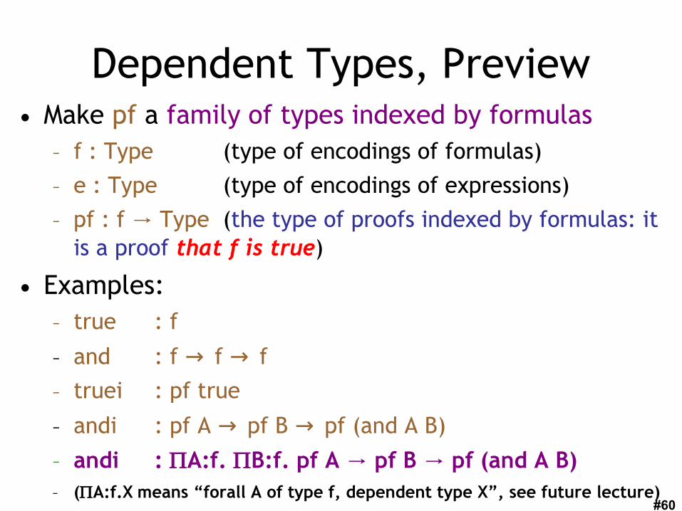
Dependent Types, Preview• Make pf a family of types indexed by formulas
– f : Type (type of encodings of formulas)
– e : Type (type of encodings of expressions)
– pf : f Type→ (the type of proofs indexed by formulas: it is a proof that f is true)
• Examples:– true : f
– and : f → f → f
– truei : pf true
– andi : pf A → pf B → pf (and A B)
– andi : A:f. B:f. pf A pf B pf (and A B)→ →– (A:f.X means “forall A of type f, dependent type X”, see future lecture)

#61
Proof Checking
• Validate proof trees by recursively checking them
• Given a proof tree X claiming to prove A && B
• Must check X : pf (and A B)
• We use “expression tree equality”, so – andel (andi “1+2=3” “x=y”) does not have type pf (3=3)
– This is already a proof system! If the proof-supplier wants to use the fact that 1+2=3 , 3=3, she can include a proof of it somewhere!
• Thus Type Checking = Proof Checking– And it’s quite easily decidable!

#62
Proof Inference Rules
• What are some rules of inference and function types for:– Or introduction
• Hint: or_introduction_left : pf A pf (or A B)→– Or elimination
– Not introduction
– Not elimination
– Implies introduction
– Implies elimination
– False elimination

#63
Bonus Question
• If we want to use Simplex to handle our Theory of Linear Inequalities, how do we handle …– Equality (x = 10)
– Negative Literals !(x <= 10)
– Disequality (x != 10)
• A slack variable converts an inequality to an equality. – Given: Ax <= b, create fresh y >= 0
– Obtain: Ax + y = b
#64
Homework
• HW2 Due Today• Wes will be away Thursday and Friday
– HW2 may not be graded before you are asked to turn in HW3. Sorry!
• HW3 Coding Hint:– You are only being asked to code up the
“check this candidate model against the Theories and add new clauses if it doesn't work” part of SMT.
Recommended