Theis Lange
Asymptotic Theory in Financial TimeSeries Models with Conditional
Heteroscedasticity
Ph.D. Thesis
2008
Thesis Advisor: Professor Anders Rahbek
University of Copenhagen
Thesis Committee: Professor Thomas Mikosch
University of Copenhagen
Professor H. Peter Boswijk
Universiteit van Amsterdam
Associate Professor Christian Dahl
University of Aarhus
Department of Mathematical Sciences
Faculty of Science
University of Copenhagen


Preface
This thesis is written in partial fulfillment of the requirements for achieving the
Ph.D. degree in mathematical statistics at the Department of Mathematical Sci-
ences under the Faculty of Science at the University of Copenhagen. The work has
been completed from May 2005 to May 2008 under the supervision of Professor
Anders Rahbek, University of Copenhagen.
The overall topic of the present thesis is econometrics and especially the field of
volatility modeling and non-linear cointegration. The work is almost exclusively
theoretical, but both the minor included empirical studies as well as the potential
applications are to financial data. The thesis is composed of four separate papers
suitable for submission to journals on theoretical econometrics. Even though all
four papers concern volatility modeling they are quite different in terms of both
scope and choice of perspective. In many ways this mirrors the many inspiring,
but different people I have met during the last three years. As a natural conse-
quence of this dispersion of focus there are some notational discrepancies among
the four papers. Each paper should therefore be read independently.
Financial support from the Danish Social Sciences Research Council grant no.
2114-04-0001, which have made this work possible is gratefully acknowledge. In
addition I thank the Danish Ministry of Science, Technology, and Innovation for
awarding me the 2007 EliteForsk travel grant. I have on several occasions visited
the Center for Research in Econometric Analysis of Time Series (CREATES) at
the University of Aarhus and I thank them for their hospitality and support.
I would like to take this opportunity to thank my supervisor Professor Anders
Rahbek for generously sharing his deep knowledge of the field and for countless
hours of inspiring and rewarding conversations. Furthermore, I owe much thanks
i

to Professor Tim Bollerslev, Duke University for his hospitality during my visit
to Duke University in the spring of 2007. I highly appreciate the support and
interest shown to me by many of my colleagues and indeed everybody at the
Department of Mathematical Sciences. I wish to mention in particular Anders
Tolver Jensen, Søren Tolver Jensen, and Søren Johansen. Finally, I would like to
thank friends and family and especially Tilde Hellsten, Lene Lange, and Kjeld
Sørensen.
Theis Lange
Copenhagen, May 2008
ii
Abstract
The present thesis deals with asymptotic analysis of financial time series models
with conditional heteroscedasticity. It is well-established within financial econo-
metrics that most financial time series data exhibit time varying conditional
volatility, as well as other types of non-linearities. Reflecting this, all four essays
of this thesis consider models allowing for time varying conditional volatility, or
heteroscedasticity.
Each essay is described in detail below. In the first essay a novel estimation tech-
nique is suggested to deal with estimation of parameters in the case of heavy tails
in the autoregressive (AR) model with autoregressive conditional heteroscedastic
(ARCH) innovations. The second essay introduces a new and quite general non-
linear multivariate error correction model with regime switching and discusses
a theory for inference. In this model cointegration can be analyzed with mul-
tivariate ARCH innovations. In the third essay properties of the much applied
heteroscedastic robust Wald test statistic is studied in the context of the AR-
ARCH model with heavy tails. Finally, in the fourth essay, it is shown that
the stylized fact that almost all financial time series exhibit integrated GARCH
(IGARCH), can be explained by assuming that the true data generating mecha-
nism is a continuous time stochastic volatility model.
Lange, Rahbek & Jensen (2007): Estimation and Asymptotic Inference in
the AR-ARCH Model. This paper studies asymptotic properties of the quasi-
maximum likelihood estimator (QMLE) and of a suggested modified version for
the parameters in the AR-ARCH model.
The modified QMLE (MQMLE) is based on truncation of the likelihood function
and is related to the recent so-called self-weighted QMLE in Ling (2007b). We
iii

show that the MQMLE is asymptotically normal irrespectively of the existence
of finite moments, as geometric ergodicity alone suffice. Moreover, our included
simulations show that the MQMLE is remarkably well-behaved in small samples.
On the other hand the ordinary QMLE, as is well-known, requires finite fourth
order moments for asymptotic normality. But based on our considerations and
simulations, we conjecture that in fact only geometric ergodicity and finite second
order moments are needed for the QMLE to be asymptotically normal. Finally,
geometric ergodicity for AR-ARCH processes is shown to hold under mild and
classic conditions on the AR and ARCH processes.
Lange (2008a): First and second order non-linear cointegration mod-
els. This paper studies cointegration in non-linear error correction models char-
acterized by discontinuous and regime-dependent error correction and variance
specifications. In addition the models allow for ARCH type specifications of the
variance. The regime process is assumed to depend on the lagged disequilibrium,
as measured by the norm of linear stable or cointegrating relations. The main
contributions of the paper are: i) conditions ensuring geometric ergodicity and fi-
nite second order moment of linear long run equilibrium relations and differenced
observations, ii) a representation theorem similar to Granger’s representations
theorem and a functional central limit theorem for the common trends, iii) to
establish that the usual reduced rank regression estimator of the cointegrating
vector is consistent even in this highly extended model, and iv) asymptotic nor-
mality of the parameters for fixed cointegration vector and regime parameters.
Finally, an application of the model to US term structure data illustrates the
empirical relevance of the model.
Lange (2008b): Limiting behavior of the heteroskedastic robust Wald-
test when the underlying innovations have heavy tails. This paper es-
tablishes that the usual OLS estimator of the autoregressive parameter in the
first order AR-ARCH model has a non-standard limiting distribution with a
non-standard rate of convergence if the innovations have non-finite fourth order
moments. Furthermore, it is shown that the robust t- and Wald test statistics
of White (1980) are still consistent and have the usual rate of convergence, but
a non-standard limiting distribution when the innovations have non-finite fourth
order moment. The critical values for the non-standard limiting distribution are
iv

found to be higher than the usual N(0,1) and χ21 critical values, respectively,
which implies that an acceptance of the hypothesis using the standard robust t-
or Wald tests remains valid even in the fourth order moment condition is not met.
However, the size of the test might be higher than the nominal size. Hence the
analysis presented in this paper extends the usability of the robust t- and Wald
tests of White (1980). Finally, a small empirical study illustrates the results.
Jensen & Lange (2008): On IGARCH and convergence of the QMLE for
misspecified GARCH models. We address the IGARCH puzzle by which
we understand the fact that a GARCH(1,1) model fitted by quasi maximum
likelihood estimation to virtually any financial dataset exhibit the property that
α + β is close to one. We prove that if data is generated by certain types of
continuous time stochastic volatility models, but fitted to a GARCH(1,1) model
one gets that α + β tends to one in probability as the sampling frequency is
increased. Hence, the paper suggests that the IGARCH effect could be caused by
misspecification. The result establishes that the stochastic sequence of QMLEs
do indeed behave as the deterministic parameters considered in the literature
on filtering based on misspecified ARCH models, see e.g. Nelson (1992). An
included study of simulations and empirical high frequency data is found to be
in very good accordance with the mathematical results.
v

vi

Resume
Denne afhandling omhandler asymptotisk teori for finansielle tidsrække mod-
eller med tidsvarierende betinget varians. Det er velkendt indenfor finansiel
økonometri, at de fleste finansielle tidsrækker udviser tidsafhængig betinget var-
ians og andre type af ikke-lineariteter. I lyset af dette, analyser alle fire artikler
i denne afhandling modeller, der tillader sadanne.
Hver artikel er beskrevet mere uddybende i de følgende afsnit. I den første artikel
introduceres en ny estimationsteknik, der kan handtere parameterestimation un-
der tungt halede innovationer i den autoregressive (AR) model med autoregressiv
betinget heteroskedastisitet (ARCH). Den anden artikel foreslar en ny og ganske
generel ikke-lineær multivariat fejlkorrektionsmodel og diskuterer desuden asymp-
totisk teori. I denne model kan kointegration analyseres med multivariate ARCH
innovationer. Med udgangspunkt i AR-ARCH modellen studeres i den tredje
artikel egenskaberne ved det meget anvendte heteroskedastisk robuste Wald test.
Den fjerde artikel udspringer af det sakaldte stylized fact, at stort set alle finan-
sielle tidsrækker udviser integreret GARCH (IGARCH) egenskaben. I artiklen
demonstreres det, at diskrete stikprøver fra kontinuert tids stokastiske volatilitets
modeller kan producere IGARCH effekten.
Lange, Rahbek & Jensen(2007): Estimation and Asymptotic Inference in
the AR-ARCH Model. Denne artikel studerer de asymptotiske egenskaber ved
quasi maksimum likelihood estimatoren (QMLE) og ved en foreslaet modificeret
version for parametrene i AR-ARCH modellen.
Den modificerede QMLE (MQMLE) er baseret pa trunkering af likelihood funk-
tionen og er relateret til den nyeligt foreslaede self-weighted QMLE i Ling (2007b).
Artiklen etablerer at MQMLE’en er asymptotisk normalfordelt uanset om inno-
vii

vationerne har endelige momenter af en bestemt orden, i det geometrisk ergod-
icitet alene er tilstrækkeligt. Det inkluderede simulationsstudie viser desuden at
MQMLE’en har bemærkelsesværdige fine egenskaber for korte dataserier. En-
delig udledes simple og klassiske betingelser pa AR og ARCH paramenterne, der
garanterer at processer genereret af modellen er geometrisk ergodiske.
Lange (2008a): First and second order non-linear cointegration models.
Artiklen omhandler kointegration i ikke-lineære fejl-korrektions modeller med
diskontinuær og regime afhængig fejl-korrektion samt variansspecifikation. Desu-
den tillader modellen ARCH specifikation af variansen. Regime processen antages
at afhænge af tidligere observationer. Artiklens hovedbidrag er: i) betingelser
der sikrer geometrisk ergidicitet og endeligt andet moment af lineære langtid-
sligevægtsrelationer og tilvækster, ii) en repræsentationssætning svarende til
Granger’s repræsentationssætning og en variant af Donsker’s sætning for de delte
stokastiske trends, iii) at etablere at den sædvanlige reducerede rank regressions
estimater af kointegrationsvektoren er konsistent selv i denne udvidede model og
iv) asymptotisk normalitet af parameterestimaterne for fast kointegrationsvektor
og regimeparametre. Den empiriske relevans af resultaterne illustreres med en
anvendelse pa amerikanske rentedata.
Lange (2008b): Limiting behavior of the heteroskedastic robust Wald-
test when the underlying innovations have heavy tails. Artiklen etablerer
at den sædvanlige OLS estimater af den autoregressive parameter i første or-
dens AR-ARCH modellen har en ikke-standard grænsefordeling med en ikke-
standard konvergensrate, nar innovationerne ikke har endeligt fjerde moment.
Desuden vises det, at de robuste t- and Wald teststørrelser (se White (1980))
er konsistente med standard konvergensrate, men ikke-standard grænsefordel-
ing nar innovationer ikke har endeligt fjerde moment. De kritiske værdier for
den etablerede grænsefordeling er højere end de tilsvarende for N(0, 1) og χ21
fordelingerne, hvilket implicerer at en hypotese accepteret ved hjælp af et stan-
dard robust t- eller Wald test forbliver accepteret selv nar innovationerne ikke
har endeligt fjerde moment. Det skal dog bemærkes, at testets størrelse kan være
højere end den nominelle størrelse. Resultaterne præsenteret i denne artikel ud-
vider dermed anvendelsen af de robuste t- og Wald tests introduceret i White
(1980). Et kort empirisk studie illustrer resultaterne.
viii

Jensen & Lange (2008): On IGARCH and convergence of the QMLE for
misspecified GARCH models. Vi adresserer IGARCH effekten, ved hvilken
vi forstar det faktum, at en GARCH(1,1), model fittet ved hjælp af quasi mak-
simum likelihood estimation til sa godt som ethvert finansielt datasæt besidder
den egenskab at α + β er tæt pa en. Vi beviser, at hvis data er genereret af
bestemte typer af kontinuer tids stokastiske volatilitets modeller, men fittet til en
GARCH(1,1) model vil α+β konvergere til en i sandsynlighed nar datafrekvensen
gar mod uendelig. Dermed indikerer artiklen, at IGARCH effekten kan være
forarsaget af misspecifikation. Resultatet etablerer ogsa at følgen af stokastiske
QMLE’ere opfører sig som de deterministiske parametre betragtet i litteraturen
omhandlende filtrering baseret pa misspecificerede ARCH modeller, se f.eks. Nel-
son (1992). Det inkluderede studie af simulationer og højfrekvent empirisk data
er i imponerende god overensstemmelse med de matematiske resultater.
ix

x

Content
Preface i
Abstract iii
Resume vii
Estimation and Asymptotic Inference in the AR-ARCH Model 1
Introduction . . . . . . . . . . . . . . . . . . . . . . . . . . . . . . . . . . . . . . . . . . . . . . . . . . . . . . . . . . . . . . .1
Properties of the AR-ARCH model . . . . . . . . . . . . . . . . . . . . . . . . . . . . . . . . . . . . . . . . 3
Estimation and asymptotic theory . . . . . . . . . . . . . . . . . . . . . . . . . . . . . . . . . . . . . . . . . 6
Simulation study . . . . . . . . . . . . . . . . . . . . . . . . . . . . . . . . . . . . . . . . . . . . . . . . . . . . . . . . . 10
Implications and summary . . . . . . . . . . . . . . . . . . . . . . . . . . . . . . . . . . . . . . . . . . . . . . . 17
Appendix . . . . . . . . . . . . . . . . . . . . . . . . . . . . . . . . . . . . . . . . . . . . . . . . . . . . . . . . . . . . . . . . 17
First and Second Order Non-Linear Cointegration Models 29
Introduction . . . . . . . . . . . . . . . . . . . . . . . . . . . . . . . . . . . . . . . . . . . . . . . . . . . . . . . . . . . . . 29
The first and second order non-linear cointegration model . . . . . . . . . . . . . . . . 32
Stability and order of integration . . . . . . . . . . . . . . . . . . . . . . . . . . . . . . . . . . . . . . . . . 36
xi

Estimation and asymptotic normality . . . . . . . . . . . . . . . . . . . . . . . . . . . . . . . . . . . . .39
An application to the interest rate spread . . . . . . . . . . . . . . . . . . . . . . . . . . . . . . . . 41
Conclusion . . . . . . . . . . . . . . . . . . . . . . . . . . . . . . . . . . . . . . . . . . . . . . . . . . . . . . . . . . . . . . . 47
Appendix . . . . . . . . . . . . . . . . . . . . . . . . . . . . . . . . . . . . . . . . . . . . . . . . . . . . . . . . . . . . . . . . 48
Limiting behavior of the heteroskedastic robust Wald test when
the underlying innovations have heavy tails 61
Introduction . . . . . . . . . . . . . . . . . . . . . . . . . . . . . . . . . . . . . . . . . . . . . . . . . . . . . . . . . . . . . 61
The AR-ARCH model . . . . . . . . . . . . . . . . . . . . . . . . . . . . . . . . . . . . . . . . . . . . . . . . . . . . 63
Limiting behavior of the OLS estimator . . . . . . . . . . . . . . . . . . . . . . . . . . . . . . . . . . 65
Limiting behavior of the robust Wald test . . . . . . . . . . . . . . . . . . . . . . . . . . . . . . . . 67
Empirical illustrations . . . . . . . . . . . . . . . . . . . . . . . . . . . . . . . . . . . . . . . . . . . . . . . . . . . . 70
Conclusion . . . . . . . . . . . . . . . . . . . . . . . . . . . . . . . . . . . . . . . . . . . . . . . . . . . . . . . . . . . . . . . 71
Appendix . . . . . . . . . . . . . . . . . . . . . . . . . . . . . . . . . . . . . . . . . . . . . . . . . . . . . . . . . . . . . . . . 72
On IGARCH and convergence of the QMLE for misspecified GARCH
models 85
Introduction . . . . . . . . . . . . . . . . . . . . . . . . . . . . . . . . . . . . . . . . . . . . . . . . . . . . . . . . . . . . . 85
Main results . . . . . . . . . . . . . . . . . . . . . . . . . . . . . . . . . . . . . . . . . . . . . . . . . . . . . . . . . . . . . .88
Illustrations . . . . . . . . . . . . . . . . . . . . . . . . . . . . . . . . . . . . . . . . . . . . . . . . . . . . . . . . . . . . . . 93
Conclusion . . . . . . . . . . . . . . . . . . . . . . . . . . . . . . . . . . . . . . . . . . . . . . . . . . . . . . . . . . . . . . . 95
Appendix . . . . . . . . . . . . . . . . . . . . . . . . . . . . . . . . . . . . . . . . . . . . . . . . . . . . . . . . . . . . . . . . 97
xii
Bibliography 117
Co-author statements 129
xiii

Estimation and Asymptotic Inferencein the AR-ARCH Model
By Theis Lange, Anders Rahbek, and Søren Tolver Jensen
Department of Mathematical Sciences, University of Copenhagen
E-mail: [email protected], [email protected], and [email protected]
Abstract: This paper studies asymptotic properties of the quasi-maximum likelihoodestimator (QMLE) and of a suggested modified version for the parameters in theautoregressive (AR) model with autoregressive conditional heteroskedastic (ARCH)errors.The modified QMLE (MQMLE) is based on truncation of the likelihood functionand is related to the recent so-called self-weighted QMLE in Ling (2007b). We showthat the MQMLE is asymptotically normal irrespectively of the existence of finitemoments, as geometric ergodicity alone suffices. Moreover, our included simulationsshow that the MQMLE is remarkably well-behaved in small samples. On the otherhand the ordinary QMLE, as is well-known, requires finite fourth order moments forasymptotic normality. But based on our considerations and simulations, we conjecturethat in fact only geometric ergodicity and finite second order moments are needed forthe QMLE to be asymptotically normal. Finally, geometric ergodicity for AR-ARCHprocesses is shown to hold under mild and classic conditions on the AR and ARCHprocesses.
Keywords: ARCH; Asymptotic theory; Geometric ergodicity; QMLE; Modified
QMLE.
1 Introduction
This paper considers likelihood based inference in a general stable autoregres-
sive model with autoregressive conditional heteroskedastic errors, the AR-ARCH
model. The aim of the paper is to contribute towards relaxing the moment re-
strictions currently found in the literature, which are often not met in empirical
findings as noted in Francq & Zakoıan (2004), Ling & McAleer (2003), Ling &
Li (1998), and Weiss (1984). Common to all these is the need for law of large
number type theorems, which in turn induces the need for moment restrictions.
In the pure ARCH model (no conditional mean part) Jensen & Rahbek (2004b)
show how the parameter region in which the QMLE is asymptotically normal at
the usual root T rate, can be expanded to include even non-stationary explosive
1

processes. Adapting these techniques to the AR-ARCH model leads to the study
of estimators based on two objective functions. One is the likelihood function and
one is a censored version of the likelihood function based on censoring extreme
terms of the log-likelihood function. The first estimator is the well known quasi-
maximum likelihood function (QMLE) while the second is new and is denoted
the modified quasi-maximum likelihood function (MQMLE).
Recently, and independently of our work, Ling (2007b) provides a theoretical
study of a closely related general estimator denoted self-weighted QMLE. When
computing the self-weighted QMLE the individual terms of the log-likelihood
function are weighted such that the impact of the largest terms is decreased.
The weights suggested in Ling (2007b) are fairly complex functions of the pre-
vious observations. This contrast our censoring scheme, which can be viewed
as weighting with zero-one weights. Apart from the simplicity of our censoring
scheme the main differences are: (i) We do not assume that the process has been
initiated in the stationary distribution, but instead allow for any initial distribu-
tion. (ii) We have included a simulation study, which can provide specific advice
on selecting the proper censoring. The included simulation study shows that the
new estimator performs remarkably well and in many respects is superior to the
ordinary QMLE. Finally our paper also establishes mild conditions for geometric
ergodicity of AR-ARCH processes.
The presence of ARCH type effects in financial and macro economic time
series is a well established fact. The combination of the ARCH specification for
the conditional variance and the AR specification for the conditional mean has
many appealing features, including a better specification of the forecast variance
and the possibility of testing the presence of momentum in stock returns in a
well specified model. Recently the AR-ARCH type models have been used as
the basic ”building blocks” for Markov switching and mixture models as in e.g.
Lanne & Saikkonen (2003) and Wong & Li (2001).
The linear ARCH model model was originally introduced by Engle (1982)
and asymptotic inference for this and other ARCH models have been studied
in, e.g. Strumann & Mikosch (2006), Kristensen & Rahbek (2005), Medeiros
& Veiga (2004) Berkes, Horvath & Kokoszka (2003), Lumsdaine (1996), Lee
& Hansen (1994), and Weiss (1986). Common to these is as mentioned the
assumption that the ARCH process is suitably ergodic or stationary. Recently
2

Jensen & Rahbek (2004b) have showed that the maximum likelihood estimator of
the ARCH parameter is asymptotically normal with the same rate of convergence
even in the non-stationary explosive case. However, as we demonstrate these
results do not carry over to the AR-ARCH model due to the conditional mean
part. Asymptotic inference in the AR-ARCH model is also considered in Francq
& Zakoıan (2004), Ling & McAleer (2003), and Ling & Li (1998). The first of
these establishes consistency of the QMLE assuming only existence of a stationary
solution, but as noted the asymptotic normality results in all three references rely
on the assumption of at least finite fourth order moment.
Note finally, that a related model is the so called DAR or double autoregressive
model studied in Ling (2007a), Chan & Peng (2005), and Ling (2004), sometimes
confusingly referred to as the AR-ARCH model. It differs from the AR-ARCH
model, by not allowing the ARCH effect in the errors to vary independently of
the level of the process. In particular, a unit root in the AR mean part of the
DAR process, does not necessarily imply non-stationarity.
The paper proceeds as follows. In Section 2 the model and some impor-
tant properties including geometric ergodicity of processes generated by the AR-
ARCH model are discussed. Section 3 introduces the estimators and states the
main results. In Section 4 we use Monte Carlo methods to compare the finite
sample properties of the estimators and provide advice on how to estimate in
practice. Finally Section 5 concludes. The Appendix contains all proofs.
2 Properties of the AR-ARCH model
In this section we present the model and discuss application of a law of large
numbers to functions of the process, which is a critical tool in the asymptotic
inference. The AR(r)-ARCH(p) model is given by
yt =r∑
i=1
ρiyt−i + εt(θ) = ρ′yt−1 + εt(θ), ρ = (ρ1, ..., ρr) (1)
εt(θ) =√
ht(θ)zt (2)
ht(θ) = ω +
p∑i=1
αiε2t−i(θ), α = (α1, ..., αp)
′ (3)
3
with t = 1, ..., T , yt = (yt, ..., yt−r+1)′, and zt an i.i.d.(0,1) sequence of random
variables following a distribution P . Furthermore ρ and α denotes r and p dimen-
sional vectors, respectively. For future reference define εt(θ) = (εt(θ), ..., εt−p+1(θ))′.
As to initial values estimation and inference is conditional on (y0, ..., y1−r−p),
which is observed. The parameter vector is denoted θ = (ρ′, α′, ω)′ and the true
parameter θ0 with α0 and ω0 strictly positive and the roots of the characteristic
polynomial corresponding to (1) outside the unit circle. For notational ease we
adopt the convention εt(θ0) =: εt and ht(θ0) =: ht.
Corresponding to the model, all results regarding inference hold independently
of the values of initial values. In particular, we do not assume that the initial
values are initiated from an invariant distribution. Instead, similar to Kristensen
& Rahbek (2005) where pure ARCH models are considered, we establish geomet-
ric ergodicity of the AR-ARCH process; see also Tjøstheim (1990) for a formal
discussion of geometric ergodicity. Geometric ergodicity ensures that there ex-
ists an invariant distribution, but also as shown in Jensen & Rahbek (2007) that
the law of large numbers apply to any measurable function of current and past
values of the geometric ergodic process, independently of initial values, see (4) in
Lemma 1 below. The application of the law of large numbers is a key part of the
derivations in the next section when considering the behavior of the score and
the information. The next lemma states sufficient (and mild) conditions for geo-
metric ergodicity of the Markov chain xt = (yt−1, εt)′ which appears in the score
and information expressions. Note that the choice of yt−1 and εt in the stacked
process is not important, and for instance the same result holds with xt defined
as (yt, ..., yt−r−p+1)′ instead. Initially two sets of assumptions corresponding to
the general model and the first order model, respectively, are stated.
Assumption 1. Assume that the roots of the characteristic polynomial corre-
sponding to (1) evaluated at the true parameters are outside the unit circle and
that
p∑i=1
α0,i < 1.
Assumption 2. Assume that r = p = 1, so α and ρ are scalars, and that
E[log(α0z
2t )
]< 0 and |ρ0| < 1.
4

Lemma 1. If either Assumption 1 or 2 holds and if zt has a density f with re-
spect to the Lebesgue measure on R, which is bounded away from zero on compact
sets then the process xt = (y′t−1, ε′t)′ generated by the AR-ARCH model, is geo-
metrically ergodic. In particular there exists a stationary version and moreover
if E|g(xt, ..., xt+k)| < ∞ where expectation is taken with respect to the invariant
distribution, the Law of Large Numbers given by
limT→∞
1
T
T∑t=1
g(xt, ..., xt+k)a.s.= E [g(xt, ..., xt+k)] , (4)
holds irrespectively of the choice of initial distribution.
Note that the formulation of the lemma allows the application of the law of
large numbers to summations involving functions of the Markov chain xt even
when the xt has a non-finite expectation. The proof which utilizes the drift
criterion can be found in the Appendix. Note that in recent years evermore
general conditions for geometric ergodicity for generalized ARCH type processes
have been derived, see e.g. Francq & Zakoıan (2006), Meitz & Saikkonen (2006),
Kristensen (2005), Liebscher (2005), and the many references therein. Common
to these is however, that they do not allow for an autoregressive mean part or
belong to the category of DAR models. To the best of our knowledge the only
results regarding geometric ergodicity of processes generated by the AR-ARCH
model can be found in Cline & Pu (2004), Meitz & Saikkonen (2008), and Cline
(2007), but their conditions are considerably more restrictive than the above since
the very general setup employed does not utilize the exact specification of the
simple AR-ARCH model.
With regards to the asymptotic theory the main contribution of Lemma 1 is to
enable the use of the law of large numbers. Since the conditions of Assumption 1
imply the existence of finite second order moment, which it not needed for the first
order model, it seems to be overly restrictive. We therefore state the following
high order condition, which simply enables the use of the law of large numbers.
Assumption 3. Assume that zt has a density f with respect to the Lebesgue
measure on R, which is bounded away from zero on compact sets, that there
5

exists an invariant distribution for the Markov chain xt = (y′t−1, ε′t)′, and that
1
T
T∑t=1
g(xt, ..., xt+k)P→ E [g(xt, ..., xt+k)] as T →∞,
for any measurable functions satisfying E [g(xt, ..., xt+k)] < ∞.
This mild assumption is trivially satisfied if the drift criterion is used to es-
tablish stability of the chain. In the following we will discuss estimation and
asymptotic theory under either of the three assumptions.
3 Estimation and Asymptotic Theory
In this section we study two estimators for the parameter θ in the AR-ARCH
model. The first is the classical quasi maximum likelihood estimator (QMLE).
Second, we propose a different estimator (the MQMLE) based on a modifica-
tion of the Gaussian likelihood function which censors a few extreme observa-
tions. We show that both estimators are consistent and asymptotically normally
distributed, and illustrate this by simulations. The proofs are based on verify-
ing classical asymptotic conditions given in Lemma A.1 of the appendix. This
involves asymptotic normality of the first derivative of the likelihood functions
evaluated at the true values, convergence of the second order derivative evaluated
at the true values and finally a uniform convergence result for the second order
derivatives in a neighborhood around the true value, conditions (A.1), (A.2), and
(A.4), respectively. For both estimators we verify conditions (A.1) and (A.2) un-
der the assumption of only second order moments of the ARCH process for the
QMLE, and no moments (but under Assumption 3) for the MQMLE in Lemma 2.
The uniform convergence is established for the MQMLE without any moment re-
quirements and only the assumption of geometric ergodicity of the AR-ARCH
process is therefore needed for this estimator to be asymptotically normal. The
uniform convergence for the QMLE we can establish under the assumption of fi-
nite fourth order moment as in Ling & Li (1998). However, based on simulations,
this assumption seems not essential at all and the result is conjectured to hold
for the QMLE with only second order moments assumed to be finite.
Thus for the MQMLE consistency and normality holds independently of exis-
6

tence of any finite moments, only existence of a stationary invariant distribution
is needed. In addition, the MQMLE have some nice finite sample properties as
studied in the simulations. In particular, for the estimator of the autoregressive
parameter ρ the finite sample distribution corresponding to the MQMLE approxi-
mates more rapidly the asymptotic normal one than the finite sample distribution
of the QMLE of ρ. Furthermore the bias when estimating the ARCH parame-
ter α is smaller when using the MQMLE than when using the classical QMLE.
Of course since we are ignoring potentially useful information by censoring, the
asymptotic variance for the MQMLE will be higher than for the QMLE.
We will consider the estimators based on minimizing the following functions
LiT (θ) =
1
T
T∑t=1
lit(θ) where lit(θ) = γit
(log ht(θ) +
ε2t (θ)
ht(θ)
),
for i = 0, 1 and with
γ0t = 1, and γ1
t = 1|yt−1|<M,...,|yt−r−p|<M (5)
for any positive constant M . The QMLE denoted θ0T and the MQMLE denoted
θ1T will be the estimators based on minimizing L0
T and L1T , respectively.
The MQMLE estimator differs from the QMLE by introducing censoring.
Clearly, the role of the censoring depends on the tail behavior of yt. Davis &
Mikosch (1998) show that under the assumptions of Lemma 1 the invariant dis-
tribution for εt is regularly varying with some index λ, and by Lange (2006) the
invariant distribution for yt is regularly varying with the same index. The inter-
pretation of the tail index is, that the AR-ARCH process has finite moments of all
orders below λ, but E|yt|λ = ∞ or, equivalently, that the density of the invariant
distribution of yt behaves like |yt|−λ−1 for |yt| large. Hence the probability of get-
ting extreme observations is closely related to moment restrictions on the ARCH
process. And since large observations provide the most precise estimates of the
autoregressive parameter ρ, we have that if the probability of getting extreme
observations becomes too large the QMLE has a non-standard (faster) rate of
convergence. This is confirmed by the fact that when the second order moment
of εt tends to infinity the asymptotic variance of the QMLE tends to zero (the
exact expressions can be found in Conjecture 1). Unlike the QMLE the MQMLE
7

censors away these extreme observations and is therefore asymptotically normal
without any moment restrictions (see Theorem 1).
In practice, based on the simulations, we propose to use a censoring constant
M which corresponds to censoring away at most 5% of the terms in the likelihood
function (see Section 4 for further discussion). This choice is similar to the choice
in the threshold- and change-point literature where for testing a priori certain
quantiles of the observations are assumed to be in each of the regimes, see Hansen
(1996, 1997). Note that if M is chosen in a data dependent fashion it may formally
only depend on some finite number of observations. While this is crucial from a
mathematical point of view, it is of no importance in practice.
The last part of this section contains the formal versions of our results.
Lemma 2. Under either Assumption 1, 2, or 3 and the additional assumption
that zt has a a symmetric distribution with E [(z2t − 1)2] = κ < ∞ and density
with respect to the Lebesgue measure, which is bounded on compact sets, the score
and the observed information satisfy
√TDL1
T (θ0)D→ N(0, Ω1
S)
D2L1T (θ0)
P→ Ω1I .
If the true parameter θ0 is such that in addition to the above the ARCH process
has finite second order moment it holds that
√TDL0
T (θ0)D→ N(0, Ω0
S)
D2L0T (θ0)
P→ Ω0I .
The matrices ΩiS and Ωi
I > 0 are positive definite block diagonal and the exact
expressions can be found in the appendix.
The notation defined in this lemma will be used throughout the rest of the
paper. We can now state our main results regarding the MQMLE. Note that the
proof can be found in the Appendix.
Theorem 1. Under the assumptions of Lemma 2 regarding L1T there exists a
fixed open neighborhood U = U(θ0) of θ0 such that with probability tending to
one as T →∞, L1T (θ) has a unique minimum point θ1
T in U . Furthermore θ1T is
8

consistent and asymptotically Gaussian,
√T (θ1
T − θ0)D→ N(0, (Ω1
I)−1Ω1
S(Ω1I)−1).
If zt is indeed Gaussian we have κ = 2 and therefore
(ΩiI)−1Ωi
S(ΩiI)−1 = 2(Ωi
I)−1
for i = 0, 1. Note that Theorem 1 is a local result in the sense that it only
guarantees the existence of a small neighborhood around the true parameter
value in which the function L1T (θ) has a unique minimum point, denoted θ1
T ,
which is consistent and asymptotically Gaussian. In contrast to this Ling (2007b)
establishes consistency and asymptotic normality over an arbitrary compact set.
However, unlike Ling (2007b) we do not work with a compact parameter set
during the estimation and hence our focus is on local behavior.
In the next section we provide numerical results, which indicate that the
QMLE is asymptotically normal with an asymptotic variance given by Lemma A.1
and Lemma 2 as long as the ARCH process has finite second order moment.
The required uniform convergence for the QMLE we can establish under the
assumption of finite fourth order moment as in Ling & Li (1998). However,
based on simulations, this assumption seems not essential at all and the result is
conjectured to hold for the QMLE with only second order moments assumed to
be finite. Hence we put forward the following conjecture.
Conjecture 1. Under the assumptions of Lemma 2 regarding L0T there exists a
fixed open neighborhood U = U(θ0) of θ0 such that with probability tending to one
as T → ∞, the likelihood function L0T (θ) has a unique minimum point θ0
T in U .
Furthermore θ0T is consistent and asymptotically Gaussian,
√T (θ0
T − θ0)D→ N(0, (Ω0
I)−1Ω0
S(Ω0I)−1).
It should be noted that consistency of the QMLE has been established in
Francq & Zakoıan (2004) in which they also discuss (p. 613) whether the QMLE
might indeed be asymptotically normal under the mild assumption of finite second
order moment of the innovations. However, the result has still not been formally
established.
9
4 Simulation Study
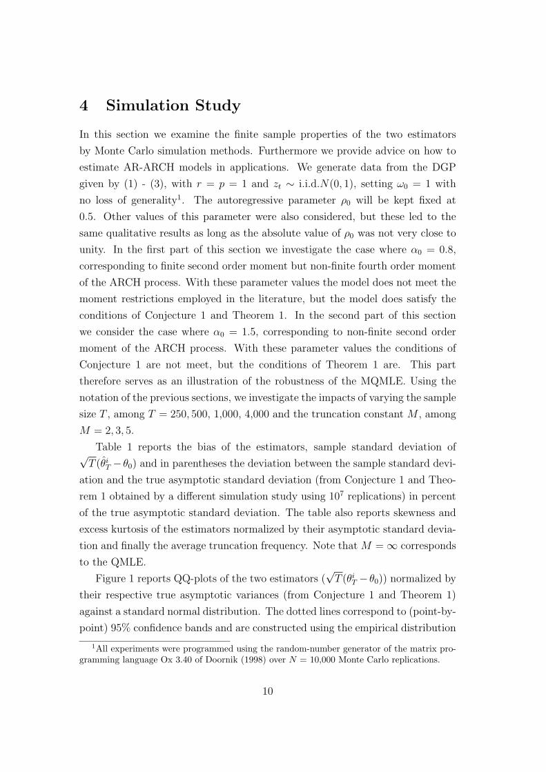
In this section we examine the finite sample properties of the two estimators
by Monte Carlo simulation methods. Furthermore we provide advice on how to
estimate AR-ARCH models in applications. We generate data from the DGP
given by (1) - (3), with r = p = 1 and zt ∼ i.i.d.N(0, 1), setting ω0 = 1 with
no loss of generality1. The autoregressive parameter ρ0 will be kept fixed at
0.5. Other values of this parameter were also considered, but these led to the
same qualitative results as long as the absolute value of ρ0 was not very close to
unity. In the first part of this section we investigate the case where α0 = 0.8,
corresponding to finite second order moment but non-finite fourth order moment
of the ARCH process. With these parameter values the model does not meet the
moment restrictions employed in the literature, but the model does satisfy the
conditions of Conjecture 1 and Theorem 1. In the second part of this section
we consider the case where α0 = 1.5, corresponding to non-finite second order
moment of the ARCH process. With these parameter values the conditions of
Conjecture 1 are not meet, but the conditions of Theorem 1 are. This part
therefore serves as an illustration of the robustness of the MQMLE. Using the
notation of the previous sections, we investigate the impacts of varying the sample
size T , among T = 250, 500, 1,000, 4,000 and the truncation constant M , among
M = 2, 3, 5.
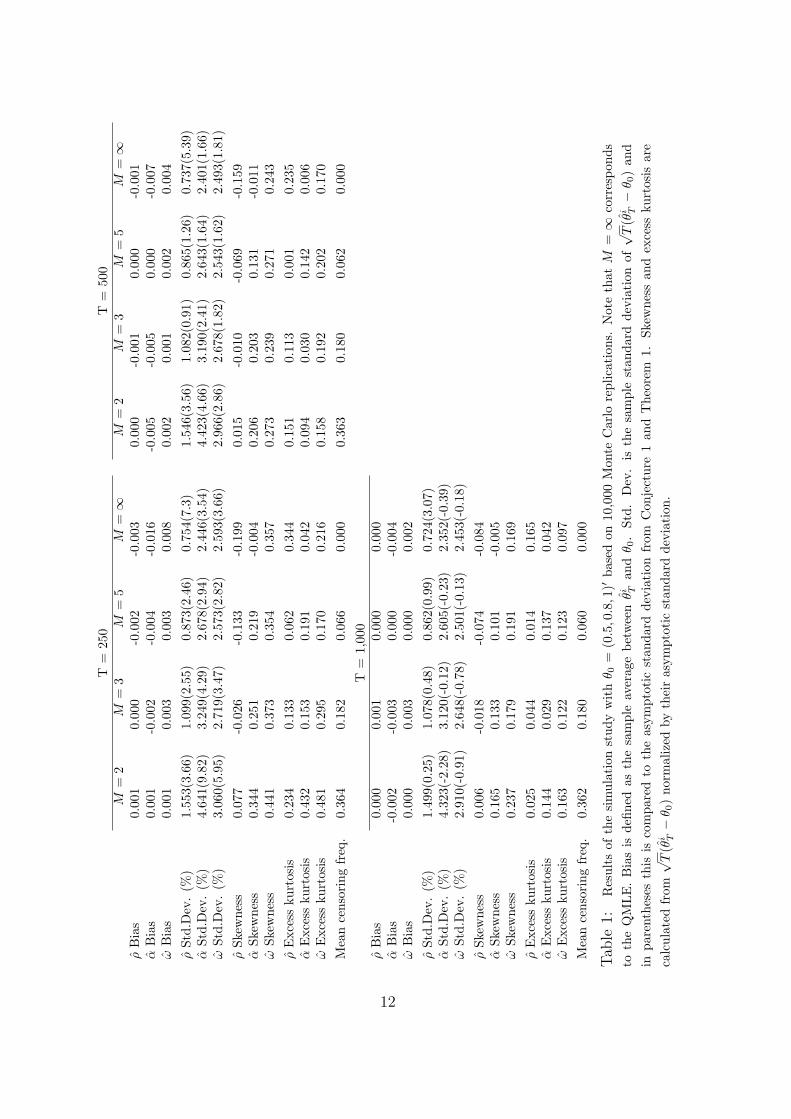
Table 1 reports the bias of the estimators, sample standard deviation of√T (θi
T − θ0) and in parentheses the deviation between the sample standard devi-
ation and the true asymptotic standard deviation (from Conjecture 1 and Theo-
rem 1 obtained by a different simulation study using 107 replications) in percent
of the true asymptotic standard deviation. The table also reports skewness and
excess kurtosis of the estimators normalized by their asymptotic standard devia-
tion and finally the average truncation frequency. Note that M = ∞ corresponds
to the QMLE.
Figure 1 reports QQ-plots of the two estimators (√
T (θiT − θ0)) normalized by
their respective true asymptotic variances (from Conjecture 1 and Theorem 1)
against a standard normal distribution. The dotted lines correspond to (point-by-
point) 95% confidence bands and are constructed using the empirical distribution
1All experiments were programmed using the random-number generator of the matrix pro-gramming language Ox 3.40 of Doornik (1998) over N = 10,000 Monte Carlo replications.
10

functions. The normalization allows one to compare how close the finite sample
distribution is to the asymptotic distribution directly between the MQMLE and
the QMLE.
We will first consider the properties of the QMLE of the autoregressive pa-
rameter. Recall that known asymptotic results only guarantees consistency, see
Francq & Zakoıan (2004), but not asymptotic normality since the ARCH process
has non-finite fourth order moment when α0 = 0.8. However, both the QQ-plot
and the numeric results of Table 1 indicate that the estimator based on L0T (the
maximum likelihood estimator) is asymptotically normal distributed with the
claimed asymptotic variance. This is in good accordance with Lemma 2, which
states that both the first- and second derivatives of L0T evaluated at the true
values have the right limits as long as the ARCH process has finite second order
moment. This forms the motivation for Conjecture 1. The plots and tables also
confirm that the QMLE of the ARCH parameters α and ω are asymptotically
Gaussian.
Next we will compare the performance of the two estimators of the autoregres-
sive parameter. From Table 1 it is noted that the observed standard deviation,
skewness, and excess kurtosis of the normalized estimator ρ1T are consistently
closer to their true asymptotic values than those of the maximum likelihood esti-
mator. Furthermore from Figure 1 it is evident that the finite sample distribution
of the MQMLE is ”closer” to the claimed normal distribution than the finite sam-
ple distribution of the QMLE. Note that the left part of the confidence bands
for the two estimators are non-overlapping, which indicates that the observed
difference is statistically significant. This is true for all values of the trunca-
tion constant M , but is most evident when M is small. From Table 1 it it also
clear that the asymptotic variance for ρ1T increases as the censoring constant is
decreased, this is due to the fact that the censoring in effect ignores useful infor-
mation. However, for M = 5, which in this case corresponds to ignoring around
5% of the terms of the likelihood function, the asymptotic standard deviation is
only around 15% larger than that of the maximum likelihood estimator.
When comparing the estimators of the ARCH parameter α, the conclusions
become less clear cut. Table 1 and Figure 1 indicate that unlike when estimating
the autoregressive parameter, the traditional QMLE is the one that approaches
its asymptotic distribution fastest (both when measured by the sample standard
11
T=
250
T=
500
M=
2M
=3
M=
5M
=∞
M=
2M
=3
M=
5M
=∞
ρB
ias
0.00
10.
000
-0.0
02-0
.003
0.00
0-0
.001
0.00
0-0
.001
αB
ias
0.00
1-0
.002
-0.0
04-0
.016
-0.0
05-0
.005
0.00
0-0
.007
ωB
ias
0.00
10.
003
0.00
30.
008
0.00
20.
001
0.00
20.
004
ρSt
d.D
ev.
(%)
1.55
3(3.
66)
1.09
9(2.
55)
0.87
3(2.
46)
0.75
4(7.
3)1.
546(
3.56
)1.
082(
0.91
)0.
865(
1.26
)0.
737(
5.39
)α
Std.
Dev
.(%
)4.
641(
9.82
)3.
249(
4.29
)2.
678(
2.94
)2.
446(
3.54
)4.
423(
4.66
)3.
190(
2.41
)2.
643(
1.64
)2.
401(
1.66
)ω
Std.
Dev
.(%
)3.
060(
5.95
)2.
719(
3.47
)2.
573(
2.82
)2.
593(
3.66
)2.
966(
2.86
)2.
678(
1.82
)2.
543(
1.62
)2.
493(
1.81
)ρ
Skew
ness
0.07
7-0
.026
-0.1
33-0
.199
0.01
5-0
.010
-0.0
69-0
.159
αSk
ewne
ss0.
344
0.25
10.
219
-0.0
040.
206
0.20
30.
131
-0.0
11ω
Skew
ness
0.44
10.
373
0.35
40.
357
0.27
30.
239
0.27
10.
243
ρE
xces
sku
rtos
is0.
234
0.13
30.
062
0.34
40.
151
0.11
30.
001
0.23
5α
Exc
ess
kurt
osis
0.43
20.
153
0.19
10.
042
0.09
40.
030
0.14
20.
006
ωE
xces
sku
rtos
is0.
481
0.29
50.
170
0.21
60.
158
0.19
20.
202
0.17
0M
ean
cens
orin
gfr
eq.
0.36
40.
182
0.06
60.
000
0.36
30.
180
0.06
20.
000
T=
1,00
0ρ
Bia
s0.
000
0.00
10.
000
0.00
0α
Bia
s-0
.002
-0.0
030.
000
-0.0
04ω
Bia
s0.
000
0.00
30.
000
0.00
2ρ
Std.
Dev
.(%
)1.
499(
0.25
)1.
078(
0.48
)0.
862(
0.99
)0.
724(
3.07
)α
Std.
Dev
.(%
)4.
323(
-2.2
8)3.
120(
-0.1
2)2.
605(
-0.2
3)2.
352(
-0.3
9)ω
Std.
Dev
.(%
)2.
910(
-0.9
1)2.
648(
-0.7
8)2.
501(
-0.1
3)2.
453(
-0.1
8)ρ
Skew
ness
0.00
6-0
.018
-0.0
74-0
.084
αSk
ewne
ss0.
165
0.13
30.
101
-0.0
05ω
Skew
ness
0.23
70.
179
0.19
10.
169
ρE
xces
sku
rtos
is0.
025
0.04
40.
014
0.16
5α
Exc
ess
kurt
osis
0.14
40.
029
0.13
70.
042
ωE
xces
sku
rtos
is0.
163
0.12
20.
123
0.09
7M
ean
cens
orin
gfr
eq.
0.36
20.
180
0.06
00.
000
Tab
le1:
Res
ults
ofth
esi
mul
atio
nst
udy
wit
hθ 0
=(0
.5,0
.8,1
)′ba
sed
on10
,000
Mon
teC
arlo
repl
icat
ions
.N
ote
that
M=∞
corr
espo
nds
toth
eQ
MLE
.B
ias
isde
fined
asth
esa
mpl
eav
erag
ebe
twee
nθi T
and
θ 0.
Std.
Dev
.is
the
sam
ple
stan
dard
devi
atio
nof√ T
(θi T−
θ 0)
and
inpa
rent
hese
sth
isis
com
pare
dto
the
asym
ptot
icst
anda
rdde
viat
ion
from
Con
ject
ure
1an
dT
heor
em1.
Skew
ness
and
exce
ssku
rtos
isar
eca
lcul
ated
from
√ T(θ
i T−
θ 0)
norm
aliz
edby
thei
ras
ympt
otic
stan
dard
devi
atio
n.
12

−4 −3 −2 −1 0 1 2 3 4
−2.
50.
02.
5E
mpi
rical
qua
ntile
s fo
r ρ
QMLE
−4 −3 −2 −1 0 1 2 3 4−
2.5
0.0
2.5
MQMLE
−4 −3 −2 −1 0 1 2 3 4
−2.
50.
02.
5E
mpi
rical
qua
ntile
s fo
r α
−4 −3 −2 −1 0 1 2 3 4
−2.
50.
02.
5
−4 −3 −2 −1 0 1 2 3 4
−2.
50.
02.
5
Standard normal
Em
piric
al q
uant
iles
for ω
−4 −3 −2 −1 0 1 2 3 4
−2.
50.
02.
5
Standard normal
Figure 1: QQ-plots of√
T (θiT − θ0) normalized by their asymptotic standard deviation
(from Conjecture 1 and Theorem 1) against a standard normal distribution. The left columncorresponds to the QMLE and the right to the MQMLE (with M = 2). The parameters arekept fixed at θ0 = (0.5, 0.8, 1)′ and T = 500 and the plot is based on 10,000 Monte Carloreplications. The dotted lines correspond to 95% confidence bands based on the empiricaldistribution function.
13
deviation, skewness, and excess kurtosis, and when inspected graphically). How-
ever, the MQMLE seems to have a lower bias than the QMLE.
Finally Table 1 and the bottom row of Figure 1 show that the estimation
of the scale parameter ω is relatively unaffected by the choice of estimator and
censoring constant.
Hence the choice of how to estimate in the AR-ARCH model depends on which
parameters that are of most interest to the problem at hand. All in all we would
suggest using the MQMLE, because it avoids the need for moment restrictions,
and selecting the censoring constant such that around 5% of the observations are
censored away, as this makes the price in the form of higher asymptotic standard
deviation fairly small.
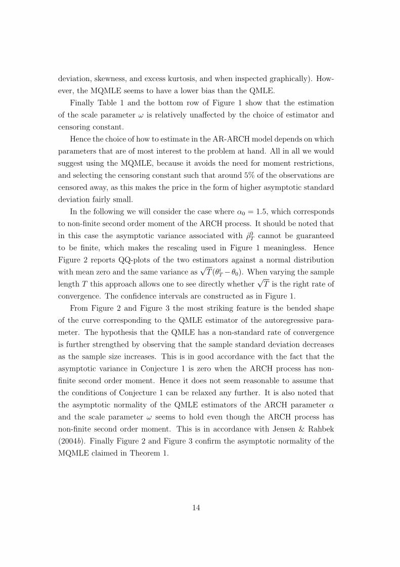
In the following we will consider the case where α0 = 1.5, which corresponds
to non-finite second order moment of the ARCH process. It should be noted that
in this case the asymptotic variance associated with ρ0T cannot be guaranteed
to be finite, which makes the rescaling used in Figure 1 meaningless. Hence
Figure 2 reports QQ-plots of the two estimators against a normal distribution
with mean zero and the same variance as√
T (θiT −θ0). When varying the sample
length T this approach allows one to see directly whether√
T is the right rate of
convergence. The confidence intervals are constructed as in Figure 1.
From Figure 2 and Figure 3 the most striking feature is the bended shape
of the curve corresponding to the QMLE estimator of the autoregressive para-
meter. The hypothesis that the QMLE has a non-standard rate of convergence
is further strengthed by observing that the sample standard deviation decreases
as the sample size increases. This is in good accordance with the fact that the
asymptotic variance in Conjecture 1 is zero when the ARCH process has non-
finite second order moment. Hence it does not seem reasonable to assume that
the conditions of Conjecture 1 can be relaxed any further. It is also noted that
the asymptotic normality of the QMLE estimators of the ARCH parameter α
and the scale parameter ω seems to hold even though the ARCH process has
non-finite second order moment. This is in accordance with Jensen & Rahbek
(2004b). Finally Figure 2 and Figure 3 confirm the asymptotic normality of the
MQMLE claimed in Theorem 1.
14

−1.5 −1.0 −0.5 0.0 0.5 1.0 1.5
−2
−1
01
2
Normal (σ: 0.419)
Em
piric
al q
uant
iles
for ρ
QMLE
−4 −2 0 2 4−
2.5
0.0
2.5
5.0
Normal (σ: 1.158)
MQMLE
−10 −5 0 5 10
−10
010
Normal (σ: 3.173)
Em
piric
al q
uant
iles
for α
−20 −10 0 10 20
−10
010
20
Normal (σ: 5.428)
−10 −5 0 5 10
−10
010
Normal (σ: 3.120)
Em
piric
al q
uant
iles
for ω
−10 −5 0 5 10
−10
010
Normal (σ: 3.561)
Figure 2: QQ-plots of√
T (θiT − θ0) against a standard normal distribution with mean zero
and the same variance as√
T (θiT − θ0). The left column corresponds to the QMLE and the
right to the MQMLE (with M = 3). The parameters are kept fixed at θ0 = (0.5, 1.5, 1)′ andT = 500 and the plot is based on 10,000 Monte Carlo replications. The dotted lines correspondto 95% confidence bands based on the empirical distribution function.
15

−1.0 −0.5 0.0 0.5 1.0
−1
01
Normal (σ: 0.328407)
Em
piric
al q
uant
iles
for ρ
QMLE
−4 −2 0 2 4−
2.5
0.0
2.5
Normal (σ: 1.150)
MQMLE
−10 −5 0 5 10
−10
−5
05
10
Normal (σ: 3.086)
Em
piric
al q
uant
iles
for α
−20 −10 0 10 20
−10
010
20
Normal (σ: 5.228)
−10 −5 0 5 10
−10
010
Normal (σ: 3.139)
Em
piric
al q
uant
iles
for ω
−10 −5 0 5 10
−10
010
Normal (σ: 3.570)
Figure 3: QQ-plots of√
T (θiT − θ0) against a standard normal distribution with mean zero
and the same variance as√
T (θiT − θ0). The left column corresponds to the QMLE and the
right to the MQMLE (with M = 3). The parameters are kept fixed at θ0 = (0.5, 1.5, 1)′ and T
= 4,000 and the plot is based on 10,000 Monte Carlo replications. The dotted lines correspondto 95% confidence bands based on the empirical distribution function.
16

5 Implications and Summary
We have initially derived minimal conditions under which processes generated
by the AR-ARCH model are geometrically ergodic. For the maximum likeli-
hood estimator in this model we have conjectured that the parameter region for
which the estimator is asymptotically normal can be extended from the fourth
order moment condition of Ling & Li (1998) to a second order moment condition.
As mentioned similar considerations have been made in Francq & Zakoıan (2004)
and Ling (2007a). The paper also suggests a different estimator (MQMLE) which
we prove to be asymptotically normal without any moment restrictions. By a
Monte Carlo study we show that the MQMLE of the autoregressive parameter
approximates its asymptotic distribution faster than the maximum likelihood es-
timator and that its asymptotic variance is only slightly larger. For the estimator
of the ARCH parameter α the gain from using the MQMLE is a slightly lower
bias, while the estimator of the scale parameter ω is unaffected by the choice of
estimator.
On the basis of our results we suggest to implement the MQMLE choosing
a censoring constant such that the observed censoring frequency is around 5%2.
In our view this provides a good balance between low standard deviation on
the estimator and a good normal approximation for the sample lengths usually
encountered in financial econometrics, however, one should also consider the use
of the estimates when deciding the estimation procedure (see the discussion in
the previous section), since the two procedures have different strengths.
A Appendix
Proof of Lemma 1. This proof can be seen as verifying the high level conditions
(CM.1)-(CM.4) in Kristensen (2005), for geometric ergodicity of general non-
linear state space models. Under Assumption 1 the result follows by combining
two well known drift criterions for autoregressive- and ARCH processes, respec-
tively. A detailed derivation can be found in Lange (2008a). The remaining part
of the proof will therefore focus on Assumption 2 where α and ρ are both scalars.
Note first that xt is a Markov chain. Using (1) - (3) twice one can express xt
2Ox code for employing both estimators discussed in this paper can be downloaded fromwww.math.ku.dk/∼lange.
17
in terms of xt−2 and the two innovations zt and zt−1 as
xt =
(ρ2
0yt−3 + zt−1(ω0 + α0ε2t−2)
1/2 + ρ0εt−2
zt(ω0 + α0(ω0 + α0ε2t−2)z
2t−1)
1/2
).
Conditional on xt−2 the map from (zt−1, zt) to xt is a bijective and all points are
regular (the determinant of the Jacobian matrix is non-zero for all points). Since
the pair (zt−1, zt) has a density with respect to the two dimensional Lebesgue mea-
sure, which is strictly positive on compacts, a classical result regarding transfor-
mations of probability measures with densities yields that the two step transition
kernel for the chain xt has strictly positive density on compact sets. By Chan &
Tong (1985) the 2-step chain is aperiodic, Lebesgue-irreducible, and all compact
sets are small.
Below we establish that the 1-step chain satisfies a drift criterion, which for
a drift function V (x) can be formulated as
E[V (xt) | xt−1 = x] ≤ aV (x) + b,
with 0 < a < 1 and b > 0. For the 2-step chain the law of the iterated expectation
yields
E[V (xt) | xt−2 = x] ≤ E[aV (xt−1) + b | xt−2 = x] ≤ a2V (x) + ab + b.
Hence the 2-step chain also satisfies a drift criterion and it is therefore geometri-
cally ergodic by Tjøstheim (1990). By Lemma 3.1 of Tjøstheim (1990) it therefore
holds that the 1-step chain is geometrically ergodic as well.
In order to establish the drift criterion for the 1-step chain define the drift
function
V (xt) = 1 + |yt−1|δ + C|εt|δ,
where C > 0 and 1 > δ > 0. Since V is continuous xt is geometrically ergodic by
the drift criterion of Tjøstheim (1990) if
E [V (xt) | xt−1]
V (xt−1)< 1, (6)
18

for all xt−1 outside some compact set K. Simple calculations yield
E [V (xt) | xt−1]
V (xt−1)=
1 + |ρ0yt−2 + εt−1|δ + C(ω0 + α0ε2t−1)
δ/2E[|zt|δ
]
V (xt−1)
≤ 1 + Cωδ/20
V (xt−1)+|ρ0|δ|yt−2|δ + (1 + Cα
δ/20 E
[|zt|δ])|εt−1|δ
V (xt−1).
With K(r) = x ∈ R2 | ‖x‖ < r the first fraction can be made arbitrarily
small outside K by choosing r large enough. Next define the function h(δ) =
αδ/20 E
[|zt|δ]and note that h(0) = 1 and h′(0) = E [log(α0z
2t )] /2. The existence of
the derivative from the right is guaranteed by Lebesgue’s Dominated Convergence
Theorem and the finite second order moment of zt. Hence by assumption there
exists a δ ∈]0, 1[ such that h(δ) < 1 and |ρ0| < 1. Therefore the constant C can
be chosen large enough such that (6) holds for all xt−1 outside the compact set
K.
Finally the law of large numbers (4) follows from Theorem 1 of Jensen &
Rahbek (2007). This completes the proof of Lemma 1.
All our asymptotic results are based on applying Lemma A.1, which follows.
Note that conditions (A.1) - (A.4) are similar to conditions stated in the literature
on asymptotic likelihood-based inference, see, e.g. Jensen & Rahbek (2004a)
Lemma 1; Lehmann (1999) Theorem 7.5.2. The difference is that (A.1) - (A.4)
avoid making assumptions on the third derivatives of the estimating function.
Lemma A.1. Consider `T (φ), which is a function of the observations X1, ..., XT
and the parameter φ ∈ Φ ⊆ Rk. Introduce furthermore φ0, which is an interior
point of Φ. Assume that `T (·) : Rk → R is two times continuously differentiable
in φ and that
(A.1) As T →∞,√
T∂`T (φ0)/∂φD→ N(0, ΩS), ΩS > 0.
(A.2) As T →∞, ∂2`T (φ0)/∂φ∂φ′P→ ΩI > 0.
(A.3) There exists a continuous function F : Rk → Rk×k such that ∂2`T (φ)/∂φ∂φ′P→ F (φ) for all φ ∈ N(φ0).
(A.4) supφ∈N(φ0) ‖∂2`T (φ)/∂φ∂φ′ − F (φ)‖ P→ 0,
where N(φ0) is a neighborhood of φ0. Then there exists a fixed open neighborhood
U(φ0) ⊆ N(φ0) of φ0 such that
19

(B.1) As T →∞ it holds that
P (there exists a minimum point φT of `T (φ) in U(φ0)) → 1
P (`T (φ) is convex in U(φ0)) → 1
P (φT is unique and solves ∂`T (φ)/∂φ = 0) → 1
(B.2) As T →∞, φTP→ φ0.
(B.3) As T →∞,√
T (φT − φ0)D→ N(0, Ω−1
I ΩSΩ−1I ).
Note that assumptions (A.3) and (A.4) could have been stated as a single
condition, but for ease of exposition in the following proofs we have chosen this
formulation.
Proof of Lemma A.1. By definition the continuous function `T (φ) attains its min-
imum on any compact set K(φ0, r) = θ | ‖φ − φ0‖ ≤ r ⊆ N(φ0). With
vφ = (φ− φ0), and φ∗ on the line from φ to φ0, Taylor’s formula gives
`T (φ)− `T (φ0) = D`T (φ0)vφ +1
2v′φD
2`T (φ∗)vφ
= D`T (φ0)vφ +1
2v′φ[ΩI + (D2`T (φ0)− ΩI)
+(D2`T (φ∗)−D2`T (φ0))]vφ. (7)
Note that
‖D2`T (φ∗)−D2`T (φ0)‖= ‖D2`T (φ∗)− F (φ∗) + (F (φ∗)− F (φ0)) + (F (φ0)−D2`T (φ0))‖≤ ‖D2`T (φ∗)− F (φ∗)‖+ ‖F (φ∗)− F (φ0)‖+ ‖F (φ0)−D2`T (φ0)‖≤ 2 sup
φ∈K(φ0,r)
‖D2`T (φ)− F (φ)‖+ supφ∈K(φ0,r)
‖F (φ)− F (φ0)‖.
The first term converges to zero as T tends to infinity by (A.4) and the last term
can be made arbitrarily small by the continuity of F . The remaining part of the
proof is identically to the proof of Lemma 1 in Jensen & Rahbek (2004a). The
only exception is that the upper bound on ‖D2`T (φ∗) −D2`T (φ0)‖ is not linear
in r, but is a function which decreases to zero as r tends to zero.
Proof of Lemma 2. We will begin by proving the part of the lemma regarding
the log-likelihood function L0T . For exposition only we initially focus on the
autoregressive parameter ρ ∈ Rr. The derivations regarding the ARCH parameter
α and the scale parameter ω are simple when compared with the ones with respect
20
to ρ and are outlined in the last part of the proof. It is also there that the
asymptotic results for the joint parameters are given.
Initially introduce some notation
εt(θ) = (εt(θ), ..., εt−p+1(θ))′, yt = (yt, ..., yt−r+1)
′, ¯yt = (yt, ..., yt−p+1)′, (8)
and A as the r by r matrix with the ARCH parameters (α) on the diagonal. The
first and second derivatives of L0T with respect to the autoregressive parameter
are given below.
∂L0T (θ)
∂ρ=
1
T
T∑t=1
2ηt(θ)
ht(θ)εt−1(θ)
′A¯yt−2 − 2εt(θ)
ht(θ)yt−1
=:1
T
T∑t=1
s(ρ)t (θ)′
∂2L0T (θ)
∂ρ2=
1
T
T∑t=1
8ηt(θ)
h2t (θ)
¯y′t−2Aεt−1(θ)εt−1(θ)′A¯yt−2
+4
h2t (θ)
¯y′t−2Aεt−1(θ)εt−1(θ)′A¯yt−2
−2ηt(θ)
ht(θ)¯y′t−2A¯yt−2 − 8εt(θ)
h2t (θ)
yt−1εt−1(θ)′A¯yt−2 +
2
ht(θ)yt−1y
′t−1,
=:1
T
T∑t=1
s(ρρ)t (θ),
where ηt(θ) =ε2t (θ)
ht(θ)− 1. Recall the notational convention that εt(θ0) =: εt etc.
Note that the sequence (s(ρ)t )T
t=1 is a Martingale difference sequence with respect
to the filtration Ft = F(yt, yt−1, ..., y0, y−1) and applying a standard CLT for Mar-
tingale differences (e.g. from Brown (1971)) leads to consider first the conditional
second order moment
1
T
T∑t=1
E[s(ρ)t s
(ρ)t′ | Ft−1
]
=4
T
T∑t=1
(κ
h2t
¯yt−2Aεt−1ε′t−1A¯y′t−2 +
1
ht
yt−1y′t−1
)
P→ 4κE
[1
h2t
¯yt−2Aεt−1ε′t−1A¯y′t−2
]+ 4E
[1
ht
yt−1y′t−1
], (9)
21

where the convergence is due to either Lemma 1 or Assumption 3. Note that
the cross products vanish since we have assumed a symmetric distribution for
zt. Before addressing the Lindeberg condition of Brown (1971) it is noted that
since the parameter region for which an ARCH(p) process has finite second order
moment is given by a sharp inequality there exists a small constant, λ, such that
it also has finite 2 + λ moment, see Lemma 3. Hence the Lindeberg condition is
satisfied as
1
T
T∑t=1
E
[‖s(ρ)
t ‖21n‖s(ρ)t ‖>δ
√To | Ft−1
]≤ 1
T 1+λ/2δλ
T∑t=1
E[‖s(ρ)
t ‖2+λ | Ft−1
]→ 0,
for all δ > 0 as T →∞, which holds since E[‖s(ρ)
t ‖2+λ]
< ∞ by Lemma 3.
By Lemma 1 it holds that
1
T
T∑t=1
s(ρρ)t
P→ 4E
[1
h2t
¯y′t−2Aεt−1ε′t−1A¯yt−2
]+ 2E
[1
ht
yt−1y′t−1
]. (10)
The necessary finiteness of the moments is easily verified by utilizing that ηt(θ0) =
z2t − 1 and ‖εt−1/h
1/2t ‖ < p/ minα01/2 < ∞.
The arguments with respect to the ARCH parameter α and the scale para-
meter ω, and hence the joint variation, are completely analogous to the ones
applied above, and use repeatedly the inequalities ‖εt−1/h1/2t ‖ < p/ minα01/2
and 1/ht < 1/ω0. For reference all first and second order derivatives are reported
at the end of the Appendix.
Turning to the result regarding L1T one notes that since γ1
t = 1|yt−1|,...,|yt−r−p−2|<Mthe moments of interest can be bounded from above as follows
E
[γ1
t
h2t
¯y′t−2Aεt−1ε′t−1A¯yt−2
]+ E
[γ0
t
ht
yt−1y′t−1
]
≤ maxα02
minα02M2 +
1
ω0
M2 < ∞.
Hence the expectations in (9) and (10) are finite and the result can be derived
using the same arguments as for L0T . Direct calculations yield the following
expressions for the matrices ΩI and ΩS.
ΩiS =
4κµi1 + 4µi
2 0 0
0 κµi3 κµi
5′
0 κµi5 κµi
4
, Ωi
I =
4µi1 + 2µi
2 0 0
0 µi3 µi
5′
0 µi5 µi
4
, (11)
22
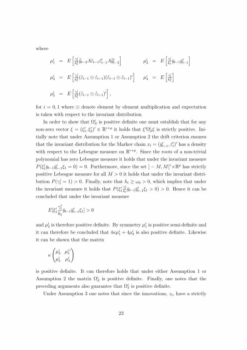
where
µi1 = E
[γi
t
h2t
¯yt−2Aεt−1ε′t−1A¯y′t−2
]µi
2 = E[
γit
htyt−1y
′t−1
]
µi3 = E
[γi
t
h2t(εt−1 ¯ εt−1)(εt−1 ¯ εt−1)
′]
µi4 = E
[γi
t
h2t
]
µi5 = E
[γi
t
h2t(εt−1 ¯ εt−1)
′],
for i = 0, 1 where ¯ denote element by element multiplication and expectation
is taken with respect to the invariant distribution.
In order to show that ΩiS is positive definite one must establish that for any
non-zero vector ξ = (ξ′1, ξ′2)′ ∈ Rr+p it holds that ξ′Ωi
Sξ is strictly positive. Ini-
tially note that under Assumption 1 or Assumption 2 the drift criterion ensures
that the invariant distribution for the Markov chain xt = (y′t−1, ε′t)′ has a density
with respect to the Lebesgue measure on Rr+p. Since the roots of a non-trivial
polynomial has zero Lebesgue measure it holds that under the invariant measure
P (ξ′1yt−1y′t−1ξ1 = 0) = 0. Furthermore, since the set ] −M, M [r×Rp has strictly
positive Lebesgue measure for all M > 0 it holds that under the invariant distri-
bution P (γit = 1) > 0. Finally, note that ht ≥ ω0 > 0, which implies that under
the invariant measure it holds that P (ξ′1γi
t
htyt−1y
′t−1ξ1 > 0) > 0. Hence it can be
concluded that under the invariant measure
E[ξ′1γi
t
ht
yt−1y′t−1ξ1] > 0
and µi2 is therefore positive definite. By symmetry µi
1 is positive semi-definite and
it can therefore be concluded that 4κµi1 + 4µi
2 is also positive definite. Likewise
it can be shown that the matrix
κ
(µi
3 µi5′
µi5 µi
4
)
is positive definite. It can therefore holds that under either Assumption 1 or
Assumption 2 the matrix ΩiS is positive definite. Finally, one notes that the
preceding arguments also guarantee that ΩiI is positive definite.
Under Assumption 3 one notes that since the innovations, zt, have a strictly
23
positive density with respect to the Lebesgue measure there exists an integer n
such that the n-step transition kernel for the Markov chain xt has strictly positive
density with respect to the Lebesgue measure. This implies that the invariant
measure also has a strictly positive density with respect to the Lebesgue measure.
By combining this with the previous arguments one has that both ΩiS and Ωi
I are
positive definite. This completes the proof of Lemma 2.
Proof of Theorem 1. The proof of Theorem 1 is based on applying Lemma A.1.
By Lemma 2 conditions (A.1) and (A.2) are satisfied. As in the proof of Lemma 2
we will focus on the vector of autoregressive parameters (ρ), and only briefly
discuss the other parameters at the end of the proof.
Introduce lower and upper values for each parameter in θ, αL < α0 < αU
(element by element), ωL < ω0 < ωU , and a positive constant δ. In terms of
these, the neighborhood N(θ0) around the true value θ0 is defined as
N(θ0) = (ρ, α, ω)′ ∈ Rr+p+1 | ‖ρ− ρ0‖ < δ, αL < α < αU , ωL < ω0 < ωU.
As in the previous proof set s(ρρ)t (θ) = ∂2l1t (θ)/∂ρ∂ρ′. In the following the exis-
tence of a stochastic variable u(ρρ)t , which satisfies
supθ∈N(θ0)
‖s(ρρ)t (θ)‖ < u
(ρρ)t (12)
and has finite expectation with respect to the invariant measure is established.
All terms of s(ρρ)t (θ) can be treated using similar arguments and we therefore only
report the derivations regarding the most involved term. Note that
supθ∈N(θ0)
γ1t ε
2t (θ)
h3t (θ)
‖¯y′t−2Aεt−1(θ)εt−1(θ)′A¯yt−2‖
≤ 2r2 maxαU2
minαL2M2γ1
t (εt(θ0)2 + 2(ρ0 ¯ ρ0 + δ2)′(yt−1 ¯ yt−1))
≤ ztC1 + C2 =: ut,
for some positive constants C1 and C2. By assumption E|ut| < ∞ and by the
triangle inequality there exists a constant K such that (12) holds with u(ρρ)t =
Kut. Hence by Lemma 1 one can define a function F as the point-by-point
probability limit of the average of the s(ρρ)t (θ)’s. Next by dominated convergence
and the continuity of the function s(ρρ)t (θ) in θ the function F is also continuous,
24

so (A.3) holds.
Finally we must verify (A.4). By (A.1) - (A.3) and Theorem 4.2.1 of Amemiya
(1985) it suffices to show
E
[sup
ρ∈N(ρ0)
‖s(ρρ)t (θ)‖
]< ∞,
which follows follows from (12). Note that Theorem 4.2.1 is applicable in our
setup by Amemiya (1985) p. 117 as the law of large numbers apply by Lemma 1.
By inspecting the remaining derivatives, reported below, it is evident that the
arguments above can be applied to all other derivatives, and applying Lemma A.1
completes the proof of Theorem 1.
Lemma 3. Under Assumption 1, 2, or 3, the assumptions from Lemma 1, and
the additional assumption that the ARCH(p) process εt has finite second order
moment, that is∑p
i=1 α0,i < 1, it holds that there exists a constant λ > 0 such
that E[|εt|2+λ] and E[|yt|2+λ] are both finite.
Proof. With out lose of generality we give the proof for the case where p = 2.
From earlier results the drift criterion is applicable. Corresponding to the ARCH
process we therefore define the Markov chain xt = (εt, ..., εt−p+1)′ and the drift
function
g(xt) = 1 + |εt|2+λ + b1|εt−1|2+λ,
for some positive constant λ. Verifying (2.4) and (2.5) of Lu (1996) establishes
the first part of the lemma. Direct calculations yield
E[g(xt) | xt−1 = (x1, x2)′]
= 1 + E[|zt|2+λ](ω0 + α0,1x1 + α0,2x2)1+λ/2 + b1|x1|2+λ
≤ 1 + E[|zt|2+λ](ω0 + α0,1 + α0,2)
1+λ/2
ω0 + α0,1 + α0,2
(ω0 + α0,1|x1|2+λ + α0,2|x2|2+λ) + b1|x1|2+λ
= 1 + c(λ)ω0 + (b1 + c(λ)α0,1)|x1|2+λ + c(λ)α0,2|x2|2+λ.
Where the inequality holds as the mapping x 7→ |x|1+λ is convex. Since the
innovations zt have finite fourth order moment it holds by bounded convergence
that c(λ) tends to 1 as λ tends to zero. Hence there exists a λ > 0 such that
c(λ)(α0,1 + α0,2) < 1 and by mimicking the proof of Theorem 1 in Lu (1996)
25
conditions (2.4) and (2.5) can be verified. The second half of the lemma follows
directly from the infinite representation of the autoregressive process yt.
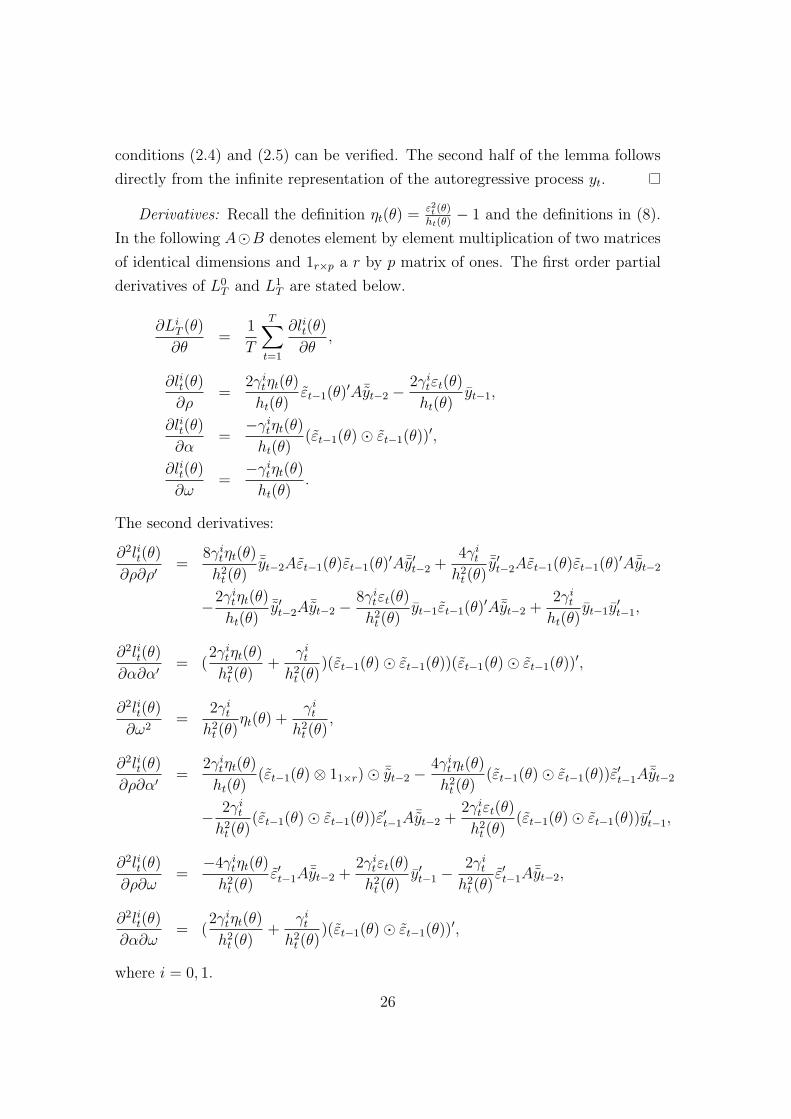
Derivatives: Recall the definition ηt(θ) =ε2t (θ)
ht(θ)− 1 and the definitions in (8).
In the following A¯B denotes element by element multiplication of two matrices
of identical dimensions and 1r×p a r by p matrix of ones. The first order partial
derivatives of L0T and L1
T are stated below.
∂LiT (θ)
∂θ=
1
T
T∑t=1
∂lit(θ)
∂θ,
∂lit(θ)
∂ρ=
2γitηt(θ)
ht(θ)εt−1(θ)
′A¯yt−2 − 2γitεt(θ)
ht(θ)yt−1,
∂lit(θ)
∂α=
−γitηt(θ)
ht(θ)(εt−1(θ)¯ εt−1(θ))
′,
∂lit(θ)
∂ω=
−γitηt(θ)
ht(θ).
The second derivatives:
∂2lit(θ)
∂ρ∂ρ′=
8γitηt(θ)
h2t (θ)
¯yt−2Aεt−1(θ)εt−1(θ)′A¯y′t−2 +
4γit
h2t (θ)
¯y′t−2Aεt−1(θ)εt−1(θ)′A¯yt−2
−2γitηt(θ)
ht(θ)¯y′t−2A¯yt−2 − 8γi
tεt(θ)
h2t (θ)
yt−1εt−1(θ)′A¯yt−2 +
2γit
ht(θ)yt−1y
′t−1,
∂2lit(θ)
∂α∂α′= (
2γitηt(θ)
h2t (θ)
+γi
t
h2t (θ)
)(εt−1(θ)¯ εt−1(θ))(εt−1(θ)¯ εt−1(θ))′,
∂2lit(θ)
∂ω2=
2γit
h2t (θ)
ηt(θ) +γi
t
h2t (θ)
,
∂2lit(θ)
∂ρ∂α′=
2γitηt(θ)
ht(θ)(εt−1(θ)⊗ 11×r)¯ ¯yt−2 − 4γi
tηt(θ)
h2t (θ)
(εt−1(θ)¯ εt−1(θ))ε′t−1A¯yt−2
− 2γit
h2t (θ)
(εt−1(θ)¯ εt−1(θ))ε′t−1A¯yt−2 +
2γitεt(θ)
h2t (θ)
(εt−1(θ)¯ εt−1(θ))y′t−1,
∂2lit(θ)
∂ρ∂ω=
−4γitηt(θ)
h2t (θ)
ε′t−1A¯yt−2 +2γi
tεt(θ)
h2t (θ)
y′t−1 −2γi
t
h2t (θ)
ε′t−1A¯yt−2,
∂2lit(θ)
∂α∂ω= (
2γitηt(θ)
h2t (θ)
+γi
t
h2t (θ)
)(εt−1(θ)¯ εt−1(θ))′,
where i = 0, 1.
26

27

28

First and second order non-linearcointegration models
By Theis Lange
Department of Mathematical Sciences, University of Copenhagen
E-mail: [email protected]
Abstract: This paper studies cointegration in non-linear error correction mod-els characterized by discontinuous and regime-dependent error correction and vari-ance specifications. In addition the models allow for autoregressive conditional het-eroscedasticity (ARCH) type specifications of the variance. The regime process isassumed to depend on the lagged disequilibrium, as measured by the norm of linearstable or cointegrating relations. The main contributions of the paper are: i) con-ditions ensuring geometric ergodicity and finite second order moment of linear longrun equilibrium relations and differenced observations, ii) a representation theoremsimilar to Granger’s representations theorem and a functional central limit theoremfor the common trends, iii) to establish that the usual reduced rank regression es-timator of the cointegrating vector is consistent even in this highly extended model,and iv) asymptotic normality of the parameters for fixed cointegration vector andregime parameters. Finally, an application of the model to US term structure dataillustrates the empirical relevance of the model.
Keywords: Cointegration, Non-linear adjustment, Regime switching, Multivariate
ARCH.
1 Introduction
Since the 1980’s the theory of cointegration has been hugely successful. Espe-
cially Granger’s representation theorem, see Johansen (1995), which provides
conditions under which non-stationary vector autoregressive (VAR) models can
exhibit stationary, stable linear combinations. This very intuitive concept of sta-
ble relations is probably the main reason why cointegration models have been so
widely applied (even outside the world of economics). For an up to date discussion
see the survey Johansen (2007).
However, recent empirical studies suggest that the adjustments to the stable re-
lations might not be adequately described by the linear specification employed
29

in the traditional cointegration model. When modeling key macroeconomic vari-
ables such as GNP, unemployment, real exchange rates, or interest rate spreads,
non-linearities can be attributed to transaction costs, which induces a band of
no disequilibrium adjustment. For a more thorough discussion see e.g. Dumas
(1992), Sercu, Uppal & Van Hulle (1995), Anderson (1997), Hendry & Ericsson
(1991), and Escribano (2004). Furthermore, policy interventions on monetary
or foreign exchange markets may also cause non-linear behavior, see Ait-Sahalia
(1996) and Forbes & Kofman (2000) among others. Such non-linearities can also
explain the problem of seemingly non-constant parameters encountered in many
applications of the usual linear models. To address this issue Balke & Fomby
(1997) suggested the threshold cointegration model, where the adjustment coeffi-
cients may switch between a specific set of values depending on the cointegrating
relations. Generalizations of this model has lead to the smooth transition models,
see Kapetanios, Shin & Snell (2006) and the references therein and the stochas-
tically switching models, see e.g. Bec & Rahbek (2004), and Dufrenot & Mignon
(2002) and the many references therein.
Parallel to this development the whole strain of literature devoted to volatility
modeling has documented that non-linearities should also be included in the spec-
ification of the variance of the innovations. A large, and ever growing, number
of autoregressive conditional heteroscedasticity (ARCH) type models, originally
introduced by Engle (1982) and generalized by Bollerslev (1986), has been sug-
gested, see e.g. Bauwens, Laurent & Rombouts (2006) for a recent discussion of
multivariate generalized ARCH models.
Motivated by these findings, this paper proposes a cointegration model, which
allows for non-linearities in both the disequilibrium adjustment and the vari-
ance specifications. The model will be referred to as the first and second order
non-linear cointegration vector autoregressive (FSNL-CVAR) model. The adjust-
ments to the stable relations are assumed to be switching according to a threshold
state process, which depends on past observations. Thus, the model extends the
concept of threshold cointegration as suggested in Balke & Fomby (1997). The
main novelty of the FSNL-CVAR model is to adopt a more general variance
specification in which the conditional variance is allowed to depend on both the
current regime as well as lagged values of the innovations, herby including an
30

important feature of financial time series.
Constructing a model which embeds many of the previously suggested models
opens up the use of likelihood based tests to assess the relative importance of these
models. For instance, does the inclusion of a regime dependent covariance matrix
render the traditional ARCH specification obsolete or vice versa? Furthermore,
since both the mean- and variance parameters depend on the current regime a
test for no regime effect in for example the mean equation can be conducted as a
simple χ2-test, since the issue of vanishing parameters under the null hypothesis,
and resulting non-standard limiting distributions see e.g. Davies (1977), has
been resolved by retaining the dependence on the regime process in the variance
specification.
The present paper derives easily verifiable conditions ensuring geometric ergod-
icity, and hence the existence of a stationary initial distribution, of the first
differences of the observations and of the linear cointegrating relationships. Sta-
bility and geometric ergodicity results form the basis for law of large numbers
theorems and are therefore an important step not only towards an understanding
of the dynamic properties of the model, but also towards the development of an
asymptotic theory. The importance of geometric ergodicity has recently been
emphasized by Jensen & Rahbek (2007), where a general law of large numbers
is shown to be a direct consequence of geometric ergodicity. It should be noted
that the conditions ensuring geometric ergodicity do not involve the parameters
of adjustment in the inner regime, corresponding to the band of no action in the
example above. The paper also derives a representation theorem corresponding
to the well known Granger representation theorem and establishes a functional
central limit theorem (FCLT) for the common trends. Finally, asymptotic nor-
mality of the parameter estimates is shown to hold under the assumption of
known cointegration vector and threshold parameters. The results are applied to
US term structure data. The empirical analysis finds clear evidence indicating
that the short-term and long-term rates only adjusts to one another when the
spread is above a certain threshold. In order to achieve a satisfactory model fit
the inclusion of ARCH effects is paramount. Hence the empirical analysis support
the need for cointegration models, which are non-linear in both the mean and the
variance. Finally, the empirical study shows that adjustments occurs through the
31
short rate only, which is in accordance with the expectation hypothesis for the
term structure.
The rest of the paper is structured as follows. Section 2 presents the model and
the necessary regularity conditions. Next Section 3 contains the results regarding
stability and order of integration. Estimation and asymptotic theory is discussed
in Section 4 and the empirical study presented in Section5. Conclusions are
presented in Section 6 and all proofs can be found in Appendix.
The following notation will be used throughout the paper. For any vector ‖ · ‖denotes the Euclidian vector norm and Ip a p-dimensional unit matrix. For some
p×r matrix β of rank r ≤ p, define the orthogonal complement β⊥ as the p×(p−r)-dimensional matrix with the property β′β⊥ = 0. The associated orthogonal
projections are given by Ip = ββ′+ β⊥β⊥ with β = β(β′β)−1. Finally εi,t denotes
the i’th coordinate of the vector εt. In Section 2 and 3 and the associated proofs
only the true parameters will be considered and the usual subscript 0 on the true
parameters will be omitted to avoid an unnecessary cumbersome notation.
2 The first and second order non-linear cointe-
gration model
In this section the model is defined and conditions for geometric ergodicity of
process generated according to the model are stated. As discussed the model
is non-linear in both the mean- and variance specification, which justifies refer-
ring to the model as the first and second order non-linear cointegration vector
autoregressive (FSNL-CVAR) model.
2.1 Non-linear adjustments
Let Xt be a p-dimensional observable stochastic process. The process is driven
by both an unobservable i.i.d. sequence νt and a zero-one valued state process
st. It is assumed that the distribution of the latter depends on lagged values of
the observable process and that νt is independent of st. The evolution of the
observable process is governed by the following generalization of the usual CVAR
32
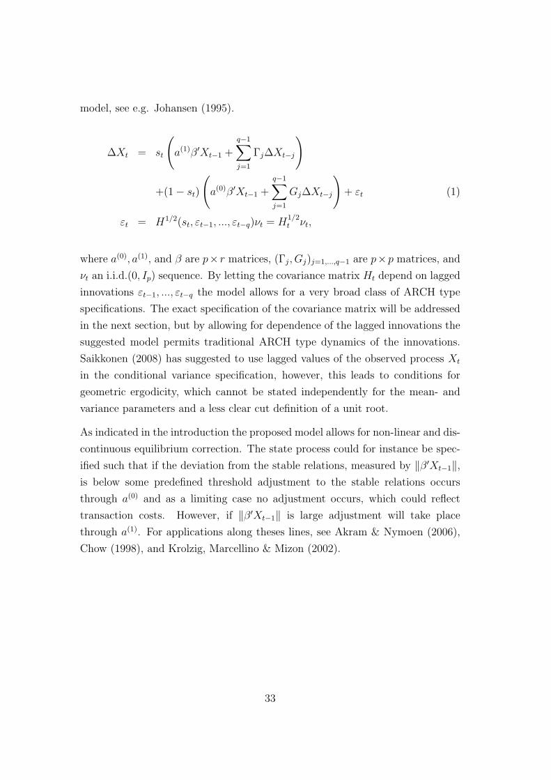
model, see e.g. Johansen (1995).
∆Xt = st
(a(1)β′Xt−1 +
q−1∑j=1
Γj∆Xt−j
)
+(1− st)
(a(0)β′Xt−1 +
q−1∑j=1
Gj∆Xt−j
)+ εt (1)
εt = H1/2(st, εt−1, ..., εt−q)νt = H1/2t νt,
where a(0), a(1), and β are p× r matrices, (Γj, Gj)j=1,...,q−1 are p×p matrices, and
νt an i.i.d.(0, Ip) sequence. By letting the covariance matrix Ht depend on lagged
innovations εt−1, ..., εt−q the model allows for a very broad class of ARCH type
specifications. The exact specification of the covariance matrix will be addressed
in the next section, but by allowing for dependence of the lagged innovations the
suggested model permits traditional ARCH type dynamics of the innovations.
Saikkonen (2008) has suggested to use lagged values of the observed process Xt
in the conditional variance specification, however, this leads to conditions for
geometric ergodicity, which cannot be stated independently for the mean- and
variance parameters and a less clear cut definition of a unit root.
As indicated in the introduction the proposed model allows for non-linear and dis-
continuous equilibrium correction. The state process could for instance be spec-
ified such that if the deviation from the stable relations, measured by ‖β′Xt−1‖,is below some predefined threshold adjustment to the stable relations occurs
through a(0) and as a limiting case no adjustment occurs, which could reflect
transaction costs. However, if ‖β′Xt−1‖ is large adjustment will take place
through a(1). For applications along theses lines, see Akram & Nymoen (2006),
Chow (1998), and Krolzig, Marcellino & Mizon (2002).
33
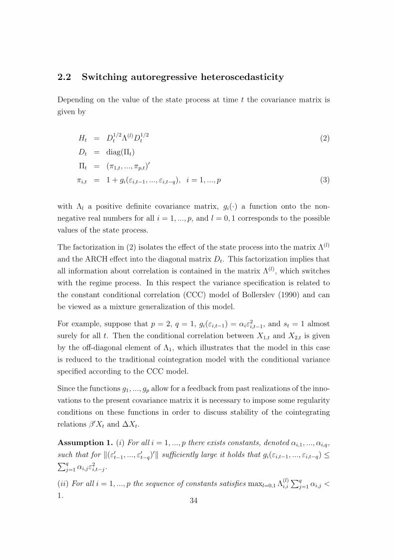
2.2 Switching autoregressive heteroscedasticity
Depending on the value of the state process at time t the covariance matrix is
given by
Ht = D1/2t Λ(l)D
1/2t (2)
Dt = diag(Πt)
Πt = (π1,t, ..., πp,t)′
πi,t = 1 + gi(εi,t−1, ..., εi,t−q), i = 1, ..., p (3)
with Λl a positive definite covariance matrix, gi(·) a function onto the non-
negative real numbers for all i = 1, ..., p, and l = 0, 1 corresponds to the possible
values of the state process.
The factorization in (2) isolates the effect of the state process into the matrix Λ(l)
and the ARCH effect into the diagonal matrix Dt. This factorization implies that
all information about correlation is contained in the matrix Λ(l), which switches
with the regime process. In this respect the variance specification is related to
the constant conditional correlation (CCC) model of Bollerslev (1990) and can
be viewed as a mixture generalization of this model.
For example, suppose that p = 2, q = 1, gi(εi,t−1) = αiε2i,t−1, and st = 1 almost
surely for all t. Then the conditional correlation between X1,t and X2,t is given
by the off-diagonal element of Λ1, which illustrates that the model in this case
is reduced to the traditional cointegration model with the conditional variance
specified according to the CCC model.
Since the functions g1, ..., gp allow for a feedback from past realizations of the inno-
vations to the present covariance matrix it is necessary to impose some regularity
conditions on these functions in order to discuss stability of the cointegrating
relations β′Xt and ∆Xt.
Assumption 1. (i) For all i = 1, ..., p there exists constants, denoted αi,1, ..., αi,q,
such that for ‖(ε′t−1, ..., ε′t−q)
′‖ sufficiently large it holds that gi(εi,t−1, ..., εi,t−q) ≤∑qj=1 αi,jε
2i,t−j.
(ii) For all i = 1, ..., p the sequence of constants satisfies maxl=0,1 Λ(l)i,i
∑qj=1 αi,j <
1.34

The assumption essentially ensures that as the lagged innovations became large
the covariance matrix responds no more vigorously than an ARCH(q) process
with finite second order moment. However, for smaller shocks the assumption
allows for a broad range of non-linear responses.
2.3 The State Process
Initially recall that the state or switching variable st is zero-one valued. Next
define the r + p(q − 1)-dimensional variable zt as
zt = (X ′t−1β, ∆X ′
t−1, ..., ∆X ′t−q+1)
′. (4)
By assumption the dynamics of the state process are given by the conditional
probability
P (st = 1 | Xt−1, ..., X0, st−1, ..., s0) = P (st = 1 | zt) ≡ p(zt). (5)
Some theoretical results regarding univariate switching autoregressive models
where the regime process is similar to (5) can be found in Gourieroux & Robert
(2006).
The transition function p(·) will be assumed to be an indicator function taking
the value one outside a bounded set as suggested by Balke & Fomby (1997).
In the transaction cost example it is intuitively clear that as the distance from
the stable relation increases so does the probability of adjustment to the stable
relation. This leads to:
Assumption 2. The transition probability p(z) defined in (5) is zero-one valued
and tends to one as ‖z‖ → ∞.
On the basis of Assumption 2 it is natural to refer to the regime where st = 0
as the inner regime and the other as the outer regime. As in Bec & Rahbek
(2004) additional inner regimes can be added without affecting the validity of the
results, the only difference being a more cumbersome notation. Extending the
model to include additional outer regimes, as in Saikkonen (2008), leads inevitable
to regularity conditions expressed in terms of the joint spectral radius of a class
35

of matrices, which are in most cases impossible to verify.
It follows that the FSNL-CVAR model allows for epochs of equilibrium adjust-
ments and epochs without. Furthermore the model allows these epochs to be
characterized by different correlation structures and have general ARCH type
variance structure. In the next section stationarity and geometric ergodicity of
β′Xt and β′⊥∆Xt are discussed.
3 Stability and order of integration
In the first part of this section conditions which ensure geometric ergodicity of
β′Xt and ∆Xt will be derived. In the second part of the section we derive a
representation theorem corresponding to the well known Granger representation
theorem and establish a FCLT for the common trends. The results presented
in this section rely on by now classical Markov chain techniques, see Meyn &
Tweedie (1993) for an introduction and definitions.
3.1 Geometric Ergodicity
Note initially that the process Xt generated by (1), (2), and (5) is not in itself
a Markov chain due to the time varying components of the covariance matrix.
Define therefore the process Vt = (X ′tβ, ∆X ′
tβ⊥)′ where the orthogonal projection
Ip = ββ′ + β⊥β′⊥, has been used. Furthermore define the stacked processes
Vt = (V ′t , ..., V
′t−q+1)
′, εt = (ε′t, ..., ε′t−q+1)
′,
and the selection matrix
ϕ = (Ip, 0p×(q−1)p)′.
By construction the process Vt is generated according to the VAR(1) model given
by
Vt = stAVt−1 + (1− st)BVt−1 + ηt, (6)
36

where ηt = ϕ(β′, β′⊥)′εt and hence is a mean zero random variable with variance
(β′, β′⊥)′Ht,st(β′, β′⊥). The matrices A and B are implicitly given by (1), see
(19) in the appendix for details. Finally the Markov chain to be considered
can be defined as Yt = (ε′t, V′t−q)
′. Note that Vt, ..., Vt−q+1 and st, ..., st−q+1 are
computable from Yt, which can be seen by first computing st−q+1 then Vt−q+1 and
repeating.
As hinted earlier it suffices to assume that the usual cointegration assumption is
satisfied for the parameters of the outer regime;
Assumption 3. Assume that the rank of a(1) and β equals r and furthermore
that there are exactly p− r roots at z = 1 for the characteristic polynomial
A(z) = Ip(1− z)− a(1)β′z −q−1∑i=1
Γi(1− z)zi, z ∈ C (7)
while the remaining roots are larger than one in absolute value.
Next the main result regarding geometric ergodicity of the Markov chain Yt will
be stated, with the central conditions expressed in terms of the matrices A and
B. In the subsequent corollaries some important special cases are considered.
Theorem 1. Assume that:
(i)For some qp× n, qp ≥ n ≥ 0 matrix µ of rank n, it holds that
(A−B)µ = 0.
(ii) The largest in absolute value of the eigenvalues of A is smaller than one.
(iii)
The stochastic state variable st is zero-one valued and the state probability
is zero-one valued and satisfies p(γ′v) → 0 as ‖γ′v‖ → ∞ with γ = µ⊥and v ∈ Rpq
(iv)νt is i.i.d.(0,Ip) and has a continuous and strictly positive density with
respect to the Lebesgue measure on Rp.
(v)The generalized ARCH functions g1, ..., gp satisfy the conditions listed in
Assumption 1.
Then Yt is a geometrically ergodic process, which has finite second order moment.
37

Furthermore there exists a distribution for Y0 such that the sequence (Yt)Tt=1 is
stationary.
The formulation of the FSNL-CVAR model is in essence a combination of the non-
linear cointegration model of Bec & Rahbek (2004) and the constant conditional
correlation model of Bollerslev (1990). It is therefore not surprising that the
following corollaries show that the stability conditions for the FSNL-CVAR model
are simply a combination of the stability conditions associated with the these two
”parent” models.
Corollary 1. Under Assumption 1, 2, and 3, and (iv) of Theorem 1 it holds
that Yt is a geometrically ergodic process with finite second order moment and
that there exists a distribution for Y0 such that the sequence (Yt)Tt=1 is stationary.
In the special case where the transition probability in (5) only depends on β′Xt
Assumption 2 does not hold. However, using Theorem 1 the following result can
be established.
Corollary 2. Consider the case where the transition probability in (5) only de-
pends on zt = β′Xt and that Γj = Gj for j = 1, ..., q − 1. Under Assumption 1,
2, and 3 and (iv) of Theorem 1 it holds that Yt is a geometrically ergodic process
with finite second order moment and that there exists a distribution for Y0 such
that the sequence (Yt)Tt=1 is stationary.
3.2 Non-stationarity
When considering linear VAR models the concept of I(1) processes is well defined,
see Johansen (1995). This is in contrast to non-linear models, such as the FSNL-
CVAR model, where there still exists considerable ambiguity as to how to define
I(1) processes. In this paper we follow Corradia, Swanson & White (2000) and
Saikkonen (2005) and simply define an I(1) process as a process for which a
functional central limit theorem (FCLT) applies. In Theorem 2 below we establish
conditions for which the (p−r) common trends of Xt have a non-degenerate long-
run variance and a FCLT applies.
38

Theorem 2. Under the assumptions of Theorem 1 the process Xt given by (1),
(2), and (5) has the representation
Xt = C
t∑i=1
(εt + (Φ(0) − Φ(1))ut) + τt, (8)
where the processes τt, see 20, and ut = (1− st)zt are stationary and zt is defined
in (4). Furthermore the parameters C, Φ(0), and Φ(1) are defined by
C = β⊥(a(1)′⊥(Ip −
k−1∑i=1
Γi)β⊥)−1a(1)′⊥, Φ(0) = (a(0), G1, ..., Gk−1),
Φ(1) = (a(1), Γ1, ..., Γk−1).
The (p − r) common trends of Xt are given by∑t
i=1 ci, where ct = a(1)′⊥(εt +
(Φ(0) − Φ(1))ut). A FCLT applies to ct − EcT , if
Υ = ψ′(
Σεε Σεu
Σuε Σuu
)ψ > 0, where ψ′ = a(1)′
⊥(Ip, Φ(0) − Φ(1)). (9)
The Σ matrices are the long run variances and the exact expression can be found
in (21).
Note that sufficient conditions for Υ being positive definite are sp(Φ(0)) = sp(Φ(1))
or a(1)′⊥Σεβ = 0.
4 Estimation and asymptotic normality
In this section it is initially established that the usual estimator in the linear
cointegrated VAR model of the cointegration vector β, which is based on reduced
rank regression (RRR), see Johansen (1995), is consistent even when data is
generated by the much more general FSNL-CVAR model. The second part of this
section considers estimation and asymptotic theory of the remaining parameters.
Define β as the usual RRR estimator of the cointegration vector defined in Jo-
hansen (1995) Theorem 6.1. Introduce the normalized estimator β given by
39

β = β(β′β)−1, where β = β(β′β)−1. Note that this normalization is clearly not
feasible in practice as the matrix β is not know, however, the purpose of the nor-
malized version is only to facilitate the formulation of the following consistency
result.
Theorem 3. Under the assumptions of Theorem 1 and the additional assumption
that Υ defined in (9) is positive definite, β is consistent and β − β = op(T1/2).
Theorem 3 suggests that once the cointegrating vector β has been estimated using
RRR the remaining parameters can be estimated by quasi-maximum likelihood
using numerical optimization. To further reduce the curse of dimensionality the
parameters Λ(1) and Λ(0) can be concentrated out of the log-likelihood function
as discussed in Bollerslev (1990). An Ox implementation of the algorithm can be
downloaded from www.math.ku.dk/∼lange.
In order to discuss asymptotic theory restrict the variance specification in (2) to
linear ARCH(q), that is replace (3) by
πi,t = 1 +
q∑j=1
αi,jε2i,t−j (10)
and define the parameter vectors
θ(1) = vec(Φ(1), Φ(0)), θ(2) = (α1,1, ..., αp,1, α2,1, ..., αp,q),
θ(3) = (vech(Λ(1))′, vech(Λ(0))′)′,
and θ = (θ(1)′, θ(2)′, θ(3)′)′. As is common let θ0 denote the true parameter value.
If the cointegration vector β and the threshold parameters are assumed known the
realization of state process is computable and the quasi log-likelihood function
to be optimized is, apart from a constant, given by
LT (θ) =1
T
T∑t=1
lt(θ), lt(θ) = − log(|Ht(θ)|)/2− εt(θ)′Ht(θ)
−1εt(θ)/2, (11)
where εt(θ) and Ht(θ) are given by (1) and (2), respectively. The assumption of
known β and λ is somewhat unsatisfactory, but at present necessary to establish
the result. Furthermore, the assumption can be partly justified by recalling that
40

estimators of both the cointegration vector and the threshold parameter are usu-
ally super consistent. The proof of the following asymptotic normality result can
be found in the appendix.
Theorem 4. Under the assumptions of Corollary 1 and the additional assump-
tion that there exists a constant δ > 0 such that E[‖εt‖4+δ] and E[‖νt‖4+δ] are
both finite and θ(2) > 0 it holds that when β and the parameters of the regime
process are kept fixed at true values there exists a fixed open neighborhood around
the true parameter N(θ0) such that with probability tending to one as T tends
to infinity, LT (θ) has a unique minimum point θT in N(θ0). Furthermore, θT is
consistent and satisfies
√T (θT − θ0)
D→ N(0, Ω−1I ΩSΩ−1
I ),
where ΩS = E[(∂lt(θ0)/∂θ)(∂lt(θ0)/∂θ′)] and ΩS = E[∂2lt(θ0)/∂θ∂θ′].
The proof is given in the appendix, where precise expressions for the asymptotic
variance are also stated.
5 An application to the interest rate spread
In this section an analysis of the spread between the long and the short U.S.
interest rates using the FSNL-CVAR model is presented. The analysis is similar
to the analysis of German interest rate spreads presented in Bec & Rahbek (2004).
However, since the FSNL-CVAR model allows for heteroscedasticity the present
analysis will employ daily data unlike the analysis in Bec & Rahbek (2004),
which is based on monthly averages. The well-known expectations hypothesis
of the term structure implies that, under costless and instantaneous portfolio
adjustments and no arbitrage the spread between the long and the short rate can
be represented as
R(k, t)−R(1, t) =1
k
k−1∑i=1
i∑j=1
Et[∆R(1, t + j)] + L(k, t), (12)
41

where R(k, t) denotes the k-period interest rate at time t, L(k, t) represents the
term premium, accounting for risk and liquidity premia, and Et[·] the expectation
conditional on the information at time t, see e.g. Bec & Rahbek (2004) for
details. Clearly, the right hand side is stable or stationary provided interest rate
changes and the the term premium are stationary (see Hall, Anderson & Granger
(1992)). In fact portfolio adjustments are neither costless nor instantaneous. It
is therefore reasonable to assume that the spread S(k, 1, t) = R(k, t) − R(1, t),
will temporarily depart from its equilibrium value given by (12). However, once
portfolio adjustments have taken place (12) will again hold. Hence, the long
and the short interest rate should be cointegrated with a cointegration vector of
β = (1,−1)′. Testing this implication of the expectations hypothesis of the term
structure has been the focus for many empirical papers, however, the results are
not clear cut. Indeed the U.S. spread is found to be stationary in e.g. Campbell &
Shiller (1987), Stock & Watson (1988), Anderson (1997), and Tzavalis & Wickens
(1998), but integrated of order 1 in e.g. Evans & Lewis (1994), Enders & Siklos
(2001), and Bec, Guayb & Guerre (2008). Note however, that when allowing for
a stationary non-linear alternative the last two papers reject the hypothesis of
non-stationarity of the U.S. spread. Indeed Anderson (1997) establishes that if
one considers homogeneous transaction costs which reduces the investors yield
on a bond by a constant amount, say λ, then one expects that the yield spread is
stationary, but non-linear, since portfolio adjustments will only occur when the
difference between the actual spread S(k, 1, t) and the value predicted by (12) is
larger in absolute value than λ.
According to Anderson’s argument the joint dynamics of short-term and long-
term interest rates could be described by the non-linear error correction model
given by (1):
∆Xt = (sta(1) + (1− st)a
(0))β′Xt +k−1∑j=1
∆Xt−j + εt, (13)
where Xt = (RSt , RL
t ), denotes the short and the long rates and the transition
function is defined in accordance with Anderson’s argument. However, as it is a
well established fact that daily interest rates exhibit considerable heteroscedas-
ticity the model must include time dependent variance as in (10).
42

1990 1992 1994 1996 1998 2000 2002 2004 2006
2.5
5.0
7.5
10.0
10 years
3 months
1990 1992 1994 1996 1998 2000 2002 2004 2006
−2
−1
0
1
2
3
Figure 1: The 3-month and 10-year interest rates (top panel) and the spreadbetween the two series adjusted for their mean (bottom panel). The dashed linesindicate the threshold λ = 1.65.
In the following the proposed FSNL-CVAR model will be applied to daily record-
ings of the U.S. 3-Month Treasury Constant Maturity Rate and the U.S. 10-Year
Treasury Constant Maturity Rate spanning the period from 1/1-1988 to 1/1-2007
yielding a total of 4,500 observations. Data have been downloaded from the web-
page of the Federal Reserve Bank of St. Louis. Following Bec & Rahbek (2004)
both series are corrected for their average and the state process is therefore given
by st = 1|SGt−1|≥λ, with SG
t−1 = β′Xt−1. This amounts to approximate the long-
run equilibrium given by (12) by the average of the actual spread, as is common
in the literature. Figure 1 depicts the data.
Initially a self-exiting threshold autoregressive (SETAR) model was fitted to the
series SGt , which indicated a threshold parameter of λ = 1.65. This value is very
close to the threshold parameter value of 1.7 reported in Bec & Rahbek (2004) for
a similar study based on monthly German interest rate data. For the remaining
part of the analysis the threshold parameter will be kept fixed at 1.65. However,
43

it should be noted that by determining the threshold parameter in such a data
dependent way the conditions for the asymptotic results given in Theorem 4 are
formally not met. In this respect, recall from the vast literature on univariate
threshold models that the threshold parameter is super-consistent and hence can
be treated as fixed when making inference on the remaining parameters, we would
expect this to hold in this case as well. Furthermore, as can be seen from (13)
the short-term parameters Γi are assumed to be identical over the two regimes,
the estimators and covariances in Theorem 4 should be adjusted accordingly.
Concerning the specification of lag lengths in (13), additional lags were included
until there were no evidence of neither autocorrelation nor additional heteroscedas-
ticity in the residuals. This lead us to retain seven lags in the mean equation and
six lags in the variance equation. The choice of lag specification was confirmed
by both the AIC as well as statistical test indicating that additional lags were
not statistically significant at the 5% level.
The parameter estimates of the mean equation are reported in the first two
columns of Table 1. Initially it is noted that the estimated parameters seem
to confirm our conjecture that when the spread is below the threshold value no
adjustment towards the equilibrium occurs. This is confirmed by testing the hy-
pothesis that a(0) = (0, 0)′, which is accepted with a p-value of 0.60 using the LR
test. In addition the estimates of a(1) indicate that long-term rates do not seem
to adjust to disequilibrium. This is confirmed by the LR test of the hypothesis
a(0)1 = a
(0)2 = a
(1)2 = 0 which cannot be rejected. The test statistic equals 2.2 cor-
responding to a p-value of 0.53. The result implies that big spreads significantly
affects the short-term rate only, which is in accordance with the expectation hy-
pothesis for the term structure. This conclusion as well as the sign of the estimate
of a(1)1 coincides with the findings of Bec & Rahbek (2004). Estimates of this re-
stricted model are reported in the last two columns of Table 1 for the parameters
of the mean equation and Table 2 for the parameters of the variance equation.
Table 2 reports the estimates of the variance equations. In order to ease com-
parison with traditional ARCH models the parametrization has been changed
slightly from the one presented in (2) to directly reporting the coefficients of the
equation Λ(1)1,1π1,t = Λ
(1)1,1 +
∑6j=1 Λ
(1)1,1αi,jε
21,t−j, which gives the conditional vari-
ance for the first element of εt when st = 1 and likewise for the other cases. It
44
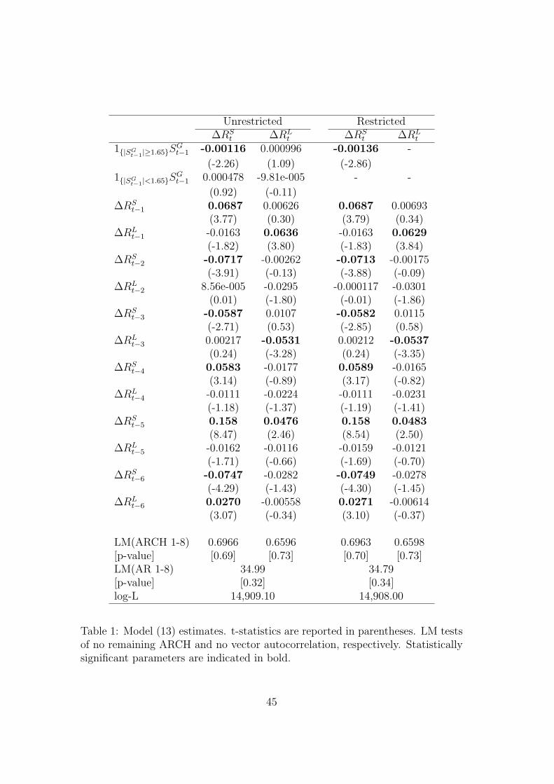
Unrestricted Restricted∆RS
t ∆RLt ∆RS
t ∆RLt
1|SGt−1|≥1.65S
Gt−1 -0.00116 0.000996 -0.00136 -
(-2.26) (1.09) (-2.86)1|SG
t−1|<1.65SGt−1 0.000478 -9.81e-005 - -
(0.92) (-0.11)∆RS
t−1 0.0687 0.00626 0.0687 0.00693(3.77) (0.30) (3.79) (0.34)
∆RLt−1 -0.0163 0.0636 -0.0163 0.0629
(-1.82) (3.80) (-1.83) (3.84)∆RS
t−2 -0.0717 -0.00262 -0.0713 -0.00175(-3.91) (-0.13) (-3.88) (-0.09)
∆RLt−2 8.56e-005 -0.0295 -0.000117 -0.0301
(0.01) (-1.80) (-0.01) (-1.86)∆RS
t−3 -0.0587 0.0107 -0.0582 0.0115(-2.71) (0.53) (-2.85) (0.58)
∆RLt−3 0.00217 -0.0531 0.00212 -0.0537
(0.24) (-3.28) (0.24) (-3.35)∆RS
t−4 0.0583 -0.0177 0.0589 -0.0165(3.14) (-0.89) (3.17) (-0.82)
∆RLt−4 -0.0111 -0.0224 -0.0111 -0.0231
(-1.18) (-1.37) (-1.19) (-1.41)∆RS
t−5 0.158 0.0476 0.158 0.0483(8.47) (2.46) (8.54) (2.50)
∆RLt−5 -0.0162 -0.0116 -0.0159 -0.0121
(-1.71) (-0.66) (-1.69) (-0.70)∆RS
t−6 -0.0747 -0.0282 -0.0749 -0.0278(-4.29) (-1.43) (-4.30) (-1.45)
∆RLt−6 0.0270 -0.00558 0.0271 -0.00614
(3.07) (-0.34) (3.10) (-0.37)
LM(ARCH 1-8) 0.6966 0.6596 0.6963 0.6598[p-value] [0.69] [0.73] [0.70] [0.73]LM(AR 1-8) 34.99 34.79[p-value] [0.32] [0.34]log-L 14,909.10 14,908.00
Table 1: Model (13) estimates. t-statistics are reported in parentheses. LM testsof no remaining ARCH and no vector autocorrelation, respectively. Statisticallysignificant parameters are indicated in bold.
45
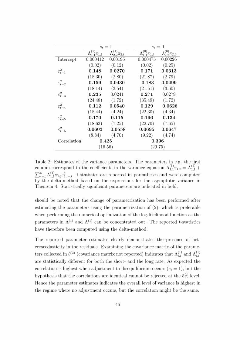
st = 1 st = 0
Λ(1)1,1π1,t Λ
(1)2,2π2,t Λ
(0)1,1π1,t λ
(0)2,2π2,t
Intercept 0.000412 0.00195 0.000475 0.00226(0.02) (0.12) (0.02) (0.25)
ε2t−1 0.148 0.0270 0.171 0.0313
(18.30) (2.80) (21.87) (2.79)ε2
t−2 0.159 0.0430 0.183 0.0499(18.14) (3.54) (21.51) (3.60)
ε2t−3 0.235 0.0241 0.271 0.0279
(24.48) (1.72) (35.49) (1.72)ε2
t−4 0.112 0.0540 0.129 0.0626(18.44) (4.24) (22.30) (4.34)
ε2t−5 0.170 0.115 0.196 0.134
(18.63) (7.25) (22.70) (7.65)ε2
t−6 0.0603 0.0558 0.0695 0.0647(8.84) (4.70) (9.22) (4.74)
Correlation 0.425 0.396(16.56) (29.75)
Table 2: Estimates of the variance parameters. The parameters in e.g. the firstcolumn correspond to the coefficients in the variance equation Λ
(1)1,1π1,t = Λ
(1)1,1 +∑6
j=1 Λ(1)1,1αi,jε
21,t−j. t-statistics are reported in parentheses and were computed
by the delta-method based on the expressions for the asymptotic variance inTheorem 4. Statistically significant parameters are indicated in bold.
should be noted that the change of parametrization has been performed after
estimating the parameters using the parametrization of (2), which is preferable
when performing the numerical optimization of the log-likelihood function as the
parameters in Λ(1) and Λ(1) can be concentrated out. The reported t-statistics
have therefore been computed using the delta-method.
The reported parameter estimates clearly demonstrates the presence of het-
eroscedasticity in the residuals. Examining the covariance matrix of the parame-
ters collected in θ(3) (covariance matrix not reported) indicates that Λ(1)i,i and Λ
(1)i,i
are statistically different for both the short- and the long rate. As expected the
correlation is highest when adjustment to disequilibrium occurs (st = 1), but the
hypothesis that the correlations are identical cannot be rejected at the 5% level.
Hence the parameter estimates indicates the overall level of variance is highest in
the regime where no adjustment occurs, but the correlation might be the same.
46

Since the parameters of the switching mechanism can be identified based solely
on the variance specification the central hypothesis a(1) = a(0), corresponding
to no switching in the mean equation, can be tested by the standard LR test
statistic, which will be asymptotically χ2 distributed with two degrees of freedom.
Thus avoiding the usual problems of unidentified parameters under the null, see
e.g. Davies (1977), Davies (1987), and the survey Lange & Rahbek (2008), often
encountered when testing no-switching hypothesis. The test statistic is 18.78 and
the hypothesis of no switching in the mean equation is therefore clearly rejected.
It should be noted that the sum of the ARCH coefficients in each column of
Table 2 are very close to one, which violates the fourth order moment condition
of Theorem 4. However, as argued in Lange, Rahbek & Jensen (2007) based on
a univariate model, we expect the asymptotic normality to hold even under a
weaker second order moment condition.
6 Conclusion
In this paper we have suggested a cointegrated vector error correction model
with a non-linear specification of both adjustments to disequilibrium and vari-
ance characterized by regime switches. Since the FSNL-CVAR model embeds
many previously suggested models, see the discussion in the introduction, it pro-
vides a framework for assessing the relative importance of these models in a
likelihood based setup. Furthermore tests of hypothesis such as linearity of the
mean equation, which previously led to non-standard limiting distributions, can
be conducted as standard χ2-tests in the FSNL-CVAR model since the state
process can be identified through the variance specification.
Using Markov chain results we derive easily verifiable conditions under which
β′Xt and ∆Xt are stable with finite second order moment and can be embedded
in a Markov chain, which is geometrically ergodic. The usefulness of this result
is enhanced by the recent work of Jensen & Rahbek (2007), which provides a
general law of large numbers assuming only geometric ergodicity. Furthermore,
a representation theorem corresponding to Granger’s representation theorem has
been derived and a functional central limit theorem for the common trends estab-
47

lished. This is utilized to show that the usual RRR estimator of Johansen (1995)
for the cointegrating vector, β, is robust to the model extensions suggested by
the FSNL-CVAR model.
Finally, we establish asymptotic normality of the estimated parameters for fixed
and known cointegration vector and threshold parameters. Applying the model
to daily recordings of the US term structure documents the empirical relevance
of the FSNL-CVAR model and the empirical results are in accordance with the
expectation hypothesis of the term structure. Specifically it is found that small
interest rate spreads are not corrected, while big ones have a significant influence
on the short rate only.
Appendix
Proof of Theorem 1
Consider initially the homogenous Markov chain Yt = (ε′t, V′t−q)
′. Before applying
the drift criterion, see e.g. Tjøstheim (1990) or Meyn & Tweedie (1993) it must
be verified that the Markov chain Yt is irreducible, aperiodic, and that compact
sets are small. In order to do so it will be verified that the 2q-step transition
kernel has a density with respect to the Lebesgue measure, which is positive and
bounded away from zero on compact sets.
Note that Vt, ..., Vt−q+1 and st, ..., st−q+1 are computable from Yt, which can be
seen by first computing st−q+1 then Vt−q+1 and repeating this procedure. With
h(· | ·) denoting a generic conditional density with respect to an appropriate
measure the 2q-step transition kernel can be rewritten as follows (for exposition
only the derivations for q = 2 are presented).
h(Yt | Yt−4) = h(εt | εt−1, Vt−2, Vt−3, Yt−4)h(εt−1 | Vt−2, Vt−3, Yt−4)
h(Vt−2 | Vt−3, Yt−4)h(Vt−3 | Yt−4)
= h(εt | st, εt−1, εt−2)h(εt−1 | st−1, εt−2, εt−3)
h(Vt−2 | st−2, Vt−3, Vt−4, εt−3, εt−4))
h(Vt−3 | st−3, Vt−4, Vt−5, εt−4, εt−5)).
48
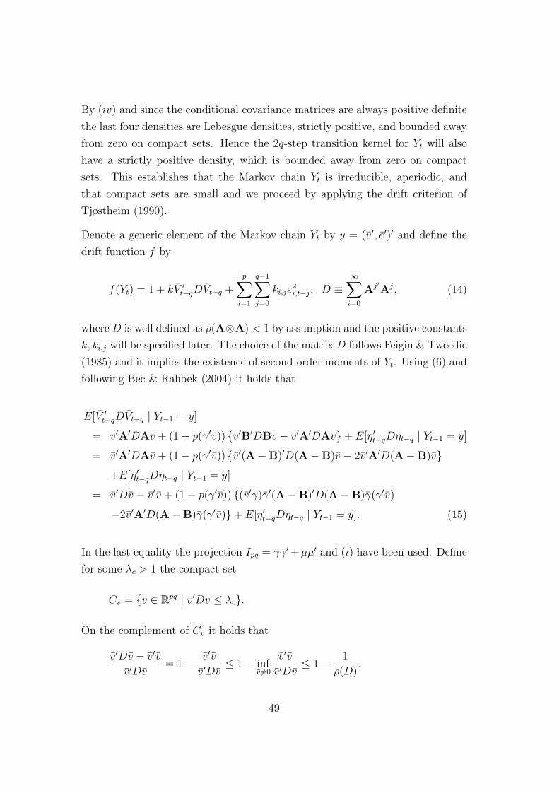
By (iv) and since the conditional covariance matrices are always positive definite
the last four densities are Lebesgue densities, strictly positive, and bounded away
from zero on compact sets. Hence the 2q-step transition kernel for Yt will also
have a strictly positive density, which is bounded away from zero on compact
sets. This establishes that the Markov chain Yt is irreducible, aperiodic, and
that compact sets are small and we proceed by applying the drift criterion of
Tjøstheim (1990).
Denote a generic element of the Markov chain Yt by y = (v′, e′)′ and define the
drift function f by
f(Yt) = 1 + kV ′t−qDVt−q +
p∑i=1
q−1∑j=0
ki,jε2i,t−j, D ≡
∞∑i=0
Aj′Aj, (14)
where D is well defined as ρ(A⊗A) < 1 by assumption and the positive constants
k, ki,j will be specified later. The choice of the matrix D follows Feigin & Tweedie
(1985) and it implies the existence of second-order moments of Yt. Using (6) and
following Bec & Rahbek (2004) it holds that
E[V ′t−qDVt−q | Yt−1 = y]
= v′A′DAv + (1− p(γ′v)) v′B′DBv − v′A′DAv+ E[η′t−qDηt−q | Yt−1 = y]
= v′A′DAv + (1− p(γ′v)) v′(A−B)′D(A−B)v − 2v′A′D(A−B)v+E[η′t−qDηt−q | Yt−1 = y]
= v′Dv − v′v + (1− p(γ′v)) (v′γ)γ′(A−B)′D(A−B)γ(γ′v)
−2v′A′D(A−B)γ(γ′v)+ E[η′t−qDηt−q | Yt−1 = y]. (15)
In the last equality the projection Ipq = γγ′+ µµ′ and (i) have been used. Define
for some λc > 1 the compact set
Cv = v ∈ Rpq | v′Dv ≤ λc.
On the complement of Cv it holds that
v′Dv − v′vv′Dv
= 1− v′vv′Dv
≤ 1− infv 6=0
v′vv′Dv
≤ 1− 1
ρ(D),
49

where ρ(·) denotes the spectral radius of a square matrix. Furthermore note that
(v′γ)γ′(A−B)′D(A−B)γ(γ′v) ³ ‖γ′v‖2
and that
2v′A′D(A−B)γ(γ′v) ³ ‖v‖ ‖γ′v‖,
where h1(x) ³ h2(x) denotes that h1(x)/h2(x) tends to a non-zero constant
as ‖x‖ tends to infinity. However, by assumption the drift function satisfies
f(y) ³ ‖y‖2 = ‖γγ′v + µµ′v‖2 + ‖e‖2 and since (1 − p(γ′v)) → 0 as ‖γ′v‖ → ∞it can be concluded that
k(1− p(γ′v)) (v′γ)γ′(A−B)′D(A−B)γ(γ′v)− 2v′A′D(A−B)γ(γ′v)f(y)
→ 0,
as ‖v‖ → ∞. Or in other words, for λc adequately large it holds that on the
complement of Cv will
kE[Vt−qDVt−q | Yt−1 = y] ≤ (1− δ∗)kv′Dv
f(y)f(y)+kE[η′t−qDηt−q | Yt−1 = y]. (16)
The constant δ∗ should be chosen such that δ∗ ∈]0, 1[ and 1ρ(D)
> δ∗ > 0. Next
consider the final term of (16). By construction it will be positive and there exists
positive constants c, ci where i = 1, ..., p such that
kE[η′t−qDηt−q | Yt−1 = y] = kE[ε′t−q(β′, β′⊥)ϕ′Dϕ(β′, β′⊥)′εt−q | Yt−1 = y]
≤ ck + k
p∑i=1
cie2i,q. (17)
As previously define the compact set Ce = e ∈ Rpq | ‖e‖2 ≤ λc. Furthermore if
50

λc is chosen large enough (v) yields that on the complement of Ce it holds that
cike2i,q +
q−1∑j=0
ki,jE[ε2i,t−j | Yt−1 = y]
= cike2i,q + ki,0E[ε2
i,t | Yt−1 = y] +
q−1∑j=1
ki,je2i,j
≤ cike2i,q + ki,0σi
(1 +
q∑j=1
αi,je2i,j
)+
q−1∑j=1
ki,je2i,j
= K + (ki,0σiαi,1 + ki,1)e2i,1 +
q−1∑j=2
(ki,0σiαi,j + ki,j)e2i,j
+(cik + ki,0σiαi,q)e2i,q (18)
for all i = 1, ..., p where K is some positive constant and σi = maxl=0,1 Λ(l)i,i . When
σi
∑qj=1 αi,j < 1 the positive constants k and ki,j can be chosen such that the
inequalities
ki,0σiαi,1 + ki,1 < ki,0
ki,0σiαi,j + ki,j < ki,j−1, j = 2, ..., q − 1
cik + ki,0σiαi,q < ki,q−1
are all satisfied, which can be seen by setting ki,0 = 1 and choosing k very small,
see Lu (1996) for details. Hence there exists a constant δ∗∗i ∈]0, 1[ such that the
coefficient of e2i,j+1 in (18) is smaller than (1− δ∗∗i )ki,j for all j = 0, ..., q − 1.
By combing (16)-(18) it can be concluded that for y outside the compact set
C = Cv × Cε will
E[f(Yt) | Yt−1 = y] ≤ (1− δ)v′Dv + (1− δ)∑p
i=1
∑q−1j=0 ki,je
2i,j+1
1 + v′Dv +∑p
i=1
∑q−1j=0 ki,je2
i,j+1
f(y)
≤ (1− δ)f(y),
where δ = min(δ∗, δ∗∗1 , ..., δ∗∗p ) > 0. Inside the compact set C the function
51

E[f(Yt) | Yt−1 = y] is continuous and hence bounded. This completes the verifi-
cation of the drift criterion.
Proof of Corollary 1
Assume without loss of generality that q = 2. Under the assumptions listed in
the corollary the coefficient matrices of (6) are given by
A =
β′a(1) − Ir + β′Γ1β β′Γ1β⊥ −β′Γ1β 0
β′⊥a(1) + β′⊥Γ1β β′⊥Γ1β⊥ −β′⊥Γ1β 0
0 0 Ir 0
0 0 0 Ip−r
, (19)
and likewise for B. Hence
(A−B) =
β′(a(1) − a(0)) + β′(Γ1 −G1)β β′(Γ1 −G1)β⊥ −β′(Γ1 −G1)β 0
β′⊥(a(1) − a(0)) + β′⊥(Γ1 −G1)β β′⊥(Γ1 −G1)β⊥ −β′⊥(Γ1 −G1)β 0
0 0 0 0
0 0 0 0
.
So the matrices γ and µ can be chosen as
γ =
Ir 0 0
0 Ip−r 0
0 0 Ir
0 0 0
, µ =
0
0
0
Ip−r
,
which satisfies µ = γ⊥ and the remaining assumptions of Theorem 1. Finally
Theorem 1 yields the desired result.
52
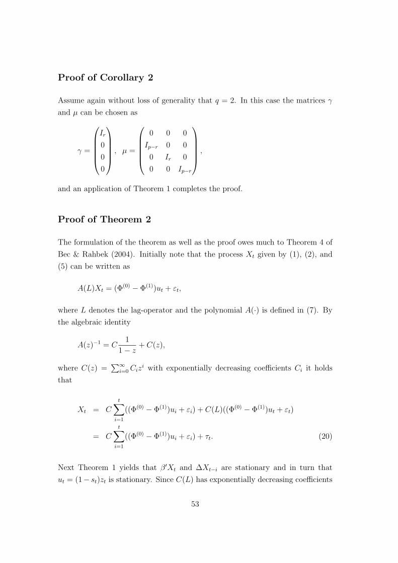
Proof of Corollary 2
Assume again without loss of generality that q = 2. In this case the matrices γ
and µ can be chosen as
γ =
Ir
0
0
0
, µ =
0 0 0
Ip−r 0 0
0 Ir 0
0 0 Ip−r
,
and an application of Theorem 1 completes the proof.
Proof of Theorem 2
The formulation of the theorem as well as the proof owes much to Theorem 4 of
Bec & Rahbek (2004). Initially note that the process Xt given by (1), (2), and
(5) can be written as
A(L)Xt = (Φ(0) − Φ(1))ut + εt,
where L denotes the lag-operator and the polynomial A(·) is defined in (7). By
the algebraic identity
A(z)−1 = C1
1− z+ C(z),
where C(z) =∑∞
i=0 Cizi with exponentially decreasing coefficients Ci it holds
that
Xt = C
t∑i=1
((Φ(0) − Φ(1))ui + εi) + C(L)((Φ(0) − Φ(1))ut + εt)
= C
t∑i=1
((Φ(0) − Φ(1))ui + εi) + τt. (20)
Next Theorem 1 yields that β′Xt and ∆Xt−i are stationary and in turn that
ut = (1− st)zt is stationary. Since C(L) has exponentially decreasing coefficients
53

it therefore holds that τt is stationary. Hence the common trends of Xt are given
by
t∑i=1
ci = a(1)′⊥
t∑i=1
((Φ(0) − Φ(1))ui + εi).
Since ‖ut‖ ≤ ‖zt‖ it holds by Theorem 17.4.2 and Theorem 17.4.4 of Meyn &
Tweedie (1993) that a FCLT applies to ct provided the long run variance Υ,
Υ = γcc(0) +∞∑
h=1
(γcc(h) + γcc(h)′), γcc(h) = Cov(ct, ct+h),
is positive definite. Note that the long run variance can be written as
Υ = ψ′(
Σεε Σεu
Σuε Σuu
)ψ, Σεu = γεu(0) +
∞∑
h=1
(γεu(h) + γεu(h)′). (21)
With similar expressions for the remaining Σ matrices.
Proof of Theorem 3
By combining Theorem 1 and Theorem 2 one can mimicking the proof of Lemma 13.1
of Johansen (1995) in order to establish the result.
Proof of Theorem 4
Before proving Theorem 4 we initially state and prove some auxiliary lemmas.
For notational ease we adopt the convention εt(θ0) = εt and likewise for other
functions of the parameter vector evaluated in the true parameters. Furthermore,
define εdt = diag(εt) and let 1(d1×d2) denote a d1 times d2 matrix of ones.
Lemma 1. Under the assumptions of Theorem 4 it holds that
1√T
T∑t=1
∂lt(θ0)
∂θ
D→ N(0, ΩS),
with ΩS = E[(∂lt(θ0)/∂θ)(∂lt(θ0)/∂θ′)] > 0 as T tends to infinity.
54
Proof. Initially note that by utilizing the diagonal structure of Dt the first deriv-
atives evaluated at the true parameters can be written as
∂lt∂θ(1)
= − ∂ε′t∂θ(1)
H−1t εt − 1
2
∂Π′t
∂θ(1)D−1
t ξt1(p×1) (22)
∂lt∂θ(2)
= −1
2
∂Π′t
∂θ(2)D−1
t ξt1(p×1) (23)
∂lt∂θ(3)
= st∂vec(Λ1)
′
∂θ(3)vec(Λ−1
1 − Λ−11 D
−1/2t εtε
′tD
−1/2t Λ−1
1 )
+(1− st)∂vec(Λ0)
′
∂θ(3)vec(Λ−1
0 − Λ−10 D
−1/2t εtε
′tD
−1/2t Λ−1
0 ) (24)
∂Π′t
∂θ(1)= 2
q∑j=1
∂ε′t−j
∂θ(1)Ajε
dt−j, Aj = diag(α1,j, ..., αp,j)
∂ε′t∂θ(1)
= stJ1zt + (1− st)J2zt
ξt = Ip − εdt H
−1t εd
t ,
where J1 is a 2p(r + p(q − 1)) times r + p(q − 1) matrix with all ones on the
first p(r + p(q− 1)) rows and zeros on the remaining rows and the matrix J2 the
opposite. Finally, the derivative of Π′t with respect to θ(2) is a block diagonal
matrix with the vectors (ε1,t−1, ..., ε1,t−q)′ to (εp,t−1, ..., εp,t−q)
′ on the diagonal
blocks.
Next, note that since the ARCH parameters are all bounded away from zero there
exists a constant k1 > 0 such that ε2i,t−j/πi,t ≤ 1/αi,j < k1 for all j = 1, ..., q. By
repeating this argument one can conclude that there exists a constant k2 such that
‖(∂Π′t/∂θD−1
t ‖ < k2. Combining this with the observations that E[‖ξt‖2] < ∞and E[‖νt‖4] < ∞ yields that E[‖∂lt/∂θ‖2] < ∞ and Ω < ∞.
For any vector c with same dimension as θ define the sequence l(1)t = c′∂lt/∂θc,
which is a martingale difference sequence with respect to the natural filtration
Ft = σ(Xt, Xt−1, ...) since E[ξt | Ft−1] = 0 and st is Ft−1 measurable. Under the
stated conditions Theorem 1, the law of large number for geometrically ergodic
time series, and the central limit of Brown (1971) yield that T−1/2∑T
t=1 l(1)t
D→N(0, c′ΩSc) and the Cramer-Wold device establishes the lemma.
The positive definiteness of ΩS can be established by noting that Theorem 1
guarantees that P (st = 1) > 0, P (st = 0) > 0, and that all elements of Yt have
55

strictly positive densities. Hence is holds that the c′Ωc = 0 if and only if c = 0
and ΩS is therefore positive definite, see Lange et al. (2007) for details.
Lemma 2. Under the conditions of Theorem 4 there exists an open neighborhood
around the true parameter value N(θ0) and a positive constant k3, such that
supθ∈N(θ0)
‖Πt(θ)′
∂θ(1)D−1
t ‖max < k3, supθ∈N(θ0)
‖Πt(θ)′
∂θ(2)D−1
t ‖max < k3,
and ‖Λ(l)−1‖max < k3 for l = 0, 1, where ‖ · ‖max denotes the max norm.
Proof. Let N(θ0) = θ ∈ Rdim(θ0) | ‖θ0 − θ‖max < δ. Next, note that by
construction any term in ∂lt(θ)
∂θ(1) will also be in the relevant part of Dt, hence it
can be concluded that if δ is sufficiently small there exists a positive constant k3
such that
supθ∈N(θ0)
‖Πt(θ)′
∂θ(1)D−1
t ‖max ≤ 1
minθ∈N(θ0) θ(2)< k3
and likewise for the derivative with respect to θ(2). Finally, note that since the
true value of both Λ(1) and Λ(0) are positive definite and the eigenvalues of a
matric is a continuous function of the matrix itself it holds that δ can be chosen
such that ‖Λ(l)−1‖max < k3 for l = 0, 1.
Proof of Theorem 4. The proof is based on a Taylor expansion of the log-likelihood
function. To avoid the need for third derivatives we will verify conditions (A.1)-
(A.4) of Lemma A.1 in Lange et al. (2007). The asymptotic normality of the
score evaluated at the true parameter values has been established in Lemma 1,
hence condition (A.1) is satisfied. By directly differentiating (22), (23), and (24)
and adopting the notation of Lemma 1 one obtains the following expressions for
the second derivatives.
56

∂2lt(θ)
∂θ(1)∂θ(1)′
= −∂εt(θ)′
∂θ(1)Ht(θ)
−1∂εt(θ)
∂θ(1)′
−1
4
∂Πt(θ)′
∂θ(1)Dt(θ)
−1(diagεt(θ)dHt(θ)
−1εt(θ)d1(p×1) − ξt + Ip)Dt(θ)
−1∂Πt(θ)
∂θ(1)′
+∂εt(θ)
′
∂θ(1)Ht(θ)
−1εt(θ)dDt(θ)
−1∂Πt(θ)
∂θ(1)′ −1
2
∂Πt(θ)′
∂θ(1)Dt(θ)
−2diagξt(θ)1(p×1)∂Πt(θ)
∂θ(1)′
−q∑
j=1
∂εt−j(θ)′
∂θ(1)AjDt(θ)
−1diagξt(θ)1(p×1)∂εt−j(θ)
∂θ(1)′
+1
2
∂Πt(θ)′
∂θ(1)Dt(θ)
−1(diagεt(θ)dHt(θ)
−11(p×1)+ εdt H
−1t )
∂εt(θ)
∂θ(1)′
∂2lt(θ)
∂θ(1)∂θ(2)′ =∂εt(θ)
′
∂θ(1)Ht(θ)
−1εt(θ)dDt(θ)
−1∂Πt(θ)
∂θ(2)′
+1
4
∂Πt(θ)′
∂θ(1)D−1
t [2diagξt(θ)1(p×1) − diagεt(θ)dHt(θ)
−1εt(θ)d1(p×1)
−εt(θ)dHt(θ)
−1εt(θ)d]D−1
t
∂Πt(θ)
∂θ(2)′
−q∑
j=1
∂εt−j(θ)′
∂θ(1)εd
t−jDt(θ)−1ξt(θ)
d ∂(Aj1(p×1))
∂θ(2)′
∂2lt(θ)
∂θ(1)∂θ(3)′ = st∂εt(θ)
′
∂θ(1)
((εt(θ)
′D−1/2t Λ−1
1 )⊗ (Λ−11 D
−1/2t )
)∂vec(Λ1)
∂θ(3)′
+(1− st)∂εt(θ)
′
∂θ(1)
((εt(θ)
′D−1/2t Λ−1
0 )⊗ (Λ−10 D
−1/2t )
)∂vec(Λ0)
∂θ(3)′
−1
2
∂Πt(θ)′
∂θ(1)D−1
t
∂(ξt(θ)1(p×1))
∂θ(3)′
∂2lt(θ)
∂θ(2)∂θ(2)′ =1
4
∂Πt(θ)′
∂θ(2)Dt(θ)
−1[2diagξt(θ)1(p×1)
−diagεt(θ)dHt(θ)
−1εt(θ)d1(p×1)+ ξt − Ip]Dt(θ)
−1∂Πt(θ)
∂θ(2)′
57

∂2lt(θ)
∂θ(2)∂θ(3)′ = −1
2
∂Πt(θ)′
∂θ(2)Dt(θ)
−1∂(ξt(θ)1(p×1))
∂θ(3)′
∂2lt(θ)
∂θ(3)∂θ(3)′ = st1
2
∂vec(Λ1)′
∂θ(3)(Λ−1
1 ⊗ Ip)[− (Λ−1
1 Dt(θ)−1/2εt(θ)εt(θ)
′Dt(θ)−1/2)⊗ Ip
−Ip ⊗ (Λ−11 Dt(θ)
−1/2εt(θ)εt(θ)′Dt(θ)
−1/2)− Ip
](Ip ⊗ Λ−1
1 )∂vec(Λ1)
∂θ(3)′
(1− st)1
2
∂vec(Λ0)′
∂θ(3)(Λ−1
0 ⊗ Ip)[− (Λ−1
0 Dt(θ)−1/2εt(θ)εt(θ)
′Dt(θ)−1/2)⊗ Ip
−Ip ⊗ (Λ−10 Dt(θ)
−1/2εt(θ)εt(θ)′Dt(θ)
−1/2) + Ip
](Ip ⊗ Λ−1
0 )∂vec(Λ0)
∂θ(3)′
∂(ξt(θ)1(p×1))
∂θ(3)′ = stεt(θ)d((εt(θ)Dt(θ)
−1/2Λ−11 )⊗ (Λ−1
1 D−1/2t )
)∂vec(Λ1)
∂θ(3)′
+(1− st)εt(θ)d((εt(θ)Dt(θ)
−1/2Λ−10 )⊗ (Λ−1
0 D−1/2t )
)∂vec(Λ0)
∂θ(3)′
By combing Theorem 1 with the law of large numbers for geometrically ergodic
time series and Lemma 2 it can be concluded that the
1
T
T∑t=1
∂2lt(θ0)
∂θ∂θ′P→ ΩI ,
as T tends to infinity. By the same arguments as in the proof of Lemma 1 ΩI is
positive definite. Hence condition (A.2) of Lemma A.1 in Lange et al. (2007) is
satisfied.
Next, let N(θ0) = θ ∈ Rdim(θ0) | ‖θ0 − θ‖max < δ denote an open neighborhood
around the true parameter value. By inspecting the second derivatives and uti-
lizing Lemma 2 it is evident that δ > 0 can be chosen such that there exists a
positive constant k4 and vector k of positive constants such that
E[ supθ∈N(θ0)
∥∥∥∂2lt(θ)
∂θ∂θ′
∥∥∥] ≤ E[k4(1 + ‖νtν′tνtν
′t‖max)k
′(z′t, ..., z′t−q)
′], (25)
which is finite by assumption. One can therefore define a function F as the point-
by-point (in θ) limit of T−1∑T
t=1 ∂2lt(θ)/∂θ∂θ′ and by dominated convergence the
function is continuous. Hence condition (A.3) is also satisfied.
58

Finally, by Theorem 4.2.1 of Amemiya (1985) the required uniform convergence
follows from (25) and condition (A.4) is therefore satisfied. Note that Theorem
4.2.1 is applicable in our setup by Amemiya (1985) p. 117 as the law of large num-
bers applies due to geometric ergodicity of the Markov chain zt. This completes
the proof.
59

60

Limiting behavior of the heteroskedasticrobust Wald test when the underlying
innovations have heavy tails
By Theis Lange
Department of Mathematical Sciences, University of Copenhagen
E-mail: [email protected]
Abstract: This paper establishes that the usual OLS estimator of the autoregressiveparameter in the first order AR-ARCH model has a non-standard limiting distributionwith a non-standard rate of convergence if the innovation has non-finite fourth ordermoment. Furthermore, it is shown that the robust t- and Wald test statistics of White(1980) are still consistent and have the usual rate of convergence, but a non-standardlimiting distribution when the innovations have non-finite fourth order moment. Thecritical values for the non-standard limiting distribution are higher than the usualN(0,1) and χ2
1 critical values, respectively, which implies that an acceptance of thehypothesis using the standard robust t- or Wald test remains valid even in the fourthorder moment condition is not met. However, the size of the test might be higher thanthe nominal size. Hence the analysis presented in this paper extends the usabilityof the robust t- and Wald tests of White (1980). Finally, a small empirical studyillustrates the results.
Keywords: ARCH; Robust t- and Wald tests; Heavy tails.
1 Introduction
Given a process (yt)Tt=1 this paper studies the OLS estimator from the regression
of yt on yt−1 when the process is assumed to be generated by a stable autoregres-
sive model with autoregressive conditional heteroskedastic errors, the AR-ARCH
model. By now the presence of ARCH type effects in financial and macro eco-
nomic time series is a well established fact. The seminal paper by Engle (1982) in
which the linear ARCH model model was originally introduced has been followed
by countless papers studying various aspects ARCH type models.
Recognizing that unmodeled heteroscedasticity in the innovations might seriously
compromise the validity of traditional t- and Wald test of the significance of
parameters estimated by OLS White (1980) introduced the heteroscedastic robust
61

t- and Wald tests. These tests are now so widely applied that they are routinely
reported by many statistical software packages. However, Whites results rely on
the innovations to have finite fourth order moment, which is often not met in
empirical studies. Recently, this limitation of the robust tests of White (1980)
has been discussed in Hamilton (2008), which provides simulations indicating that
robust tests might still be usable even when the fourth order moment condition
is not met.
In this paper we show that the robust t- and Wald test statistics have the correct
normalization, but a non-standard limiting distribution when the innovations
have non-finite fourth order moment. Indeed many of the observations based
on simulations in Hamilton (2008) can be explained by our results. The criti-
cal values for the non-standard limiting distribution are higher than the usual
N(0,1) and χ21 critical values, respectively, which implies that an acceptance of
a hypothesis using the standard robust t- or Wald test procedure remains valid
even in the fourth order moment condition is not met. However, the size of the
test might be higher than the nominal size. Hence the analysis presented in this
paper extends the usability of the robust t- and Wald tests of White (1980). In
addition the paper establishes that the OLS estimator of the autoregressive pa-
rameter will have a stable limit with a non-standard rate of convergence. As the
tools for handling stable distributions are less evolved than similar tools for nor-
mal distributions we are forced to restrict attention to a fairly simple first order
model as the true data generating mechanism. Finally, a small empirical study
shows how employing the corrected critical values can strengthen the evidence of
no correlation between consecutive movements of interest rates.
The paper proceeds as follows. In Section 2 the model and some important
properties including geometric ergodicity and tail heaviness are discussed. Sec-
tion 3 presents the limiting distributions for the OLS estimator and Section 4
states the limiting distributions for the robust t- and Wald test statistics and
discusses implications of the results on the standard testing procedures. Finally,
Section 5 contains an small empirical study and Section 6 concludes. All proofs
are contained in the Appendix.
62

2 The AR-ARCH Model
The model can be stated as
yt = ρyt−1 + εt(θ), (1)
εt(θ) =√
ht(θ)zt (2)
ht(θ) = ω + αε2t−1(θ) (3)
with t = 1, ..., T and zt an i.i.d.(0,1) sequence of random variables distributed
according to a known law, denoted P . The parameter vector is denoted θ =
(ρ, α, ω)′ and the true parameter θ0. In order to ease notation we adopt the
convention εt := εt(θ0) etc. The analysis is conditional on the initial values y0
and ε−1.
In the context of the AR-ARCH model heavy tails can be introduced either by
choosing the value of the ARCH parameter α sufficiently large while keeping the
underlying error process zt light tailed or through the tails of the underlying error
process zt. In this paper the first approach will be explored. The second approach
has been investigated in e.g. Davis & Mikosch (1998).
For a fixed value of the ARCH parameter α the tail index, denoted λ, can be
found as the unique strictly positive solution to the equation E[(αz2t )
λ/2] = 1 as
shown in Davis & Mikosch (1998) p. 2062. Note that a tail index of λ has the
implication that the ARCH process has finite moments of all orders below λ, but
E[|εt|λ] = ∞. Figure 1 depicts the correspondence between α and λ when zt is
assumed Gaussian.
Using the moment interpretation of the tail index and Figure 1 it is evident that
the ARCH process has finite fourth order moment, but non-finite second order
moment if the ARCH parameter belongs to the interval ]0.57, 1[. This part of
the parameter space will be the focus for much of the rest of the paper.
The following lemma, which has been proved in Lange, Rahbek & Jensen (2007),
establishes minimal conditions under which processes generated by the AR-ARCH
model are geometrically ergodic. Geometric ergodicity, and the laws of large
numbers implied by this concept, constitutes an important tool when establish-
63

0.50 0.75 1.00 1.25 1.50 1.75 2.00 2.25 2.50 2.75 3.00 3.25
1
2
3
4
5
α
λ
Figure 1: Correspondence between the ARCH parameter α and the tail index λ when zt isassumed Gaussian.
ing asymptotic theory, but for our intended applications it is of equal importance
that the lemma establishes minimal conditions under which there exists an initial
distribution such that the process is stationary.
Lemma 1. Assume that zt has a density f with respect to the Lebesgue measure
on R, which is bounded away from zero on compact sets and furthermore that
E[log(α0z2t )] < 0 and |ρ0| < 1
then the process xt = (yt−1, εt)′ generated by the AR-ARCH model, is geomet-
rically ergodic. In particular there exists a stationary version and moreover if
E|g(xt, ..., xt+k)| < ∞, where expectation is taken with respect to the invariant
distribution, the Law of Large Numbers given by
limT→∞
1
T
T∑t=1
g(xt, ..., xt+k)a.s.= E[g(xt, ..., xt+k)], (4)
holds irrespectively of the choice of initial distribution.
64

3 Limiting behavior of the OLS estimator
In this section the limiting behavior of the OLS estimator of the autoregressive
parameter ρ is derived under two sets of moment assumptions on the innovation
sequence. Initially this section reviews the well known result that the OLS es-
timator is asymptotically normal when the innovations have finite fourth order
moment and states precise expressions for the parameters of the limiting dis-
tribution. In the second part of this section the limiting behavior of the OLS
estimator when the innovations only have finite second order moment, is derived,
which has not previously been established in the literature. The final part of this
section discusses some implications of the limiting results.
3.1 The normal case: Finite fourth order moment
Standard techniques combined with Lemma 1 give the following result regarding
the OLS estimator of ρ when the innovations have finite fourth order moment.
Theorem 1. In addition to the assumptions in Lemma 1 assume that
(i) E[α20z
4t ] = α2
0κ < 1
(ii) and zt’s distribution is symmetric.
Then the OLS estimator of the autoregressive parameter ρ in the AR-ARCH
model given by (1) - (3) is consistent and with the following limiting distribution
√T (ρOLS − ρ0) =
T−1/2∑T
t=1 yt−1εt
T−1∑T
t=1 y2t−1
D→ N(0, Σ), (5)
where
Σ = (1− ρ20) +
(κ− 1)(1− ρ20)
2α0
(1− κα20)(1− α0ρ2
0).
The proof can be found in the appendix. As the parameter values approaches the
value (α20κ = 1) for which the ARCH process no longer have finite fourth order
moment the asymptotic variance Σ converges toward infinity. Hence one could
conjecture that in this case the limiting distribution would be a stable law with
65

a slower than square root rate of convergence. In the following section we will
prove this conjecture.
3.2 The stable case: Non-finite fourth order moment
Next, we will analyze the effect of relaxing the fourth order moment condition of
Theorem 1 to a second order condition. As conjectured this leads to both a non-
standard limiting distribution as well as non-standard rate of convergence. Since
the tools for manipulating stable laws are somewhat less evolved than similar
tools for normal distributions it is necessary to assume stationarity of the process
as geometric ergodicity does not suffice in the present version of the proof.
Theorem 2. In addition to the assumptions in Lemma 1 assume that
(i) the initial values are distributed according to the stationary distribution,
(ii) and the ARCH parameter α0 is such that the ARCH process has finite
second order moment, but non-finite fourth order moment,
then it holds that
T 1−2/λ(ρOLS − ρ0)D→ S0, (6)
where λ denotes the tail index as described in the Section 2, and S0 is a λ/2 stable
random variable, with the remaining parameters unknown.
Remark 1. The existence of a stationary distribution is guaranteed by Lemma 1.
3.3 Implications
As Theorem 1 is a standard result this section will only address the implications
of Theorem 2. Theorem 2 has the most direct implications for the construction
of confidence bands. When constructing confidence bands one needs to know
both the asymptotical distribution (usual the normal distribution) including pa-
rameters as well as the rate of convergence (usual square root T ). However, if
the true α is such that the innovation sequence does not have finite fourth order
moment Theorem 2 implies that the rate of convergence will be non-standard and
66

unknown and the parameters of the limiting distribution unknown as well. Since
the rate on convergence in Theorem 2 is slower than the usual square root T the
usually constructed confidence bands based on normality and standard rate of
convergence might be way to narrow leading to erroneous conclusions. Unfortu-
nately, since λ in unknown in practice and Theorem 2 does not include a precise
specification of the remaining parameters of the limiting stable distribution, one
cannot easily derive a corrected confidence band based on the theorem. In the
next section we will address this problem by considering the heteroskedastic ro-
bust Wald test of White (1980).
4 Limiting behavior of the robust Wald test
In this section we will examine the behavior of the heteroskedastic robust t-
and Wald tests of White (1980). The robust t-test statistic for the hypothesis
H0 : ρ0 = 0 is given by
VT =√
T (ρOLS − ρ0)( 1
T
T∑t=1
ε2t y
2t−1
)−1/2( 1
T
T∑t=1
y2t−1
),
and the robust Wald test statistic is V 2T . Under the hypothesis VT can be rewritten
as
VT =( T∑
t=1
εtεt−1
)( T∑t=1
ε2t ε
2t−1
)−1/2,
which is sometimes refereed to as a self normalizing sum. If the innovations
have finite fourth order moment it is well known, see e.g. White (1980), that VT
converges to standard normal distribution as T tends to infinity irrespectively of
possible heteroscedasticity of the innovations. This result forms the basis for the
usual robust t- and Wald test. However, if the the innovations do not have finite
fourth order moment the limiting behavior of VT has not been examined in the
litterateur. From the theory for self normalizing sums of i.i.d. random variables,
see Gine, Gotze & Mason (1997), it is known that a self normalized sum of i.i.d.
random variables converges to a normal distribution if and only if the numerator
belongs to the domain of attraction for a normal distribution. Based on this result
67
one would conjecture that VT does not have a Gaussian limiting distribution since
Theorem 2 establishes that the numerator belongs to the domain of attraction of
a stable law. Theorem 3 below formalizes this conjecture and the proof can be
found in the appendix.
Theorem 3. In addition to the assumptions in Lemma 1 assume that
(i) the initial values are distributed according to the stationary distribution,
(iii) and the ARCH parameter α0 is such that the ARCH process has finite
second order moment, but non-finite fourth order moment,
then under H0 it holds that
VTD→ S1
S1/22
(7)
where the vector (S1, S2) is jointly a λ/2 stable random variable, with the remain-
ing parameters and dependence structure unknown.
Remark 2. Inspecting the proof of Theorem 3 reveals that the result also holds
when λ ∈]0, 2[, corresponding to E[ε2t ] = ∞, but in this case Theorem 2 indicates
that ρOLS is not even consistent rendering a test for a particular value fruitless.
Corollary 1. Under the conditions of Theorem 3 the heteroskedastic robust Wald
test given by V 2T converges in distribution to S2
1/S2 where the vector (S1, S2) is
jointly a λ/2 stable random variable, with the remaining parameters and depen-
dence structure unknown.
In the following section the implications of Theorem 3 on the usual testing pro-
cedure will be discussed.
4.1 Implications for testing procedure
Arguably the most important implication of Theorem 3 and Corollary 1 is that
the normalization required to ensure a non-degenerate limiting distribution for
both the robust t- and Wald tests does not depend on a finite fourth order mo-
ment. However, since the limiting distribution is no longer Gaussian when the
innovations have non-finite fourth order moment the critical values are not the
usual ones.
68

0.1 0.2 0.3 0.4 0.5 0.6 0.7 0.8 0.9 1.0 1.1 1.2 1.3 1.4
1
2
3
4
5
6
7
8
α0
50%
70%
80%
90%
95%
97.5%
Figure 2: Quantiles for the limiting distribution for the robust Wald test statistic (S21/S2
from Corollary 1) computed by simulating from the AR-ARCH model with ρ0 = 0, ω0 = 1,and zt ∼ N(0, 1) for a range of values for α0. Each simulated path was 2,000 data points longand 100,000 Monte Carlo replications were conducted for each value of α0. The two verticalline corresponds to the values of the ARCH parameter where the process does no longer havefinite fourth order and second order moment, respectively.
In the usual Gaussian case, obtained when the innovations have finite fourth
order moment, it can directly be established by utilizing the properties of the
normal distribution that the limiting distribution for the robust t- and Wald test
statistics are nuisance parameter free (indeed even in higher order models than
the one considered in this paper). In contrast to this, it is not possible to verify
that the stable limits in Theorem 3 and Corollary 1 do not depend on additional
parameters besides the tail index, since a precise mathematical expression for
parameter values and dependence structure is not available. However, in the first
order AR-ARCH model considered in this paper the only remaining unknown
parameter is the scale parameter ω0 and the test statistic VT is clearly invariant
to the scale of the innovations.
Since the scale parameter ω0 does not affect the limiting distributions in Theo-
rem 3 and Corollary 1 the critical values for the hypothesis H0 will only depend
69

and the ARCH parameter α0. Based on simulations Figure 2 illustrates how the
critical values change as the ARCH parameter is increased.
From Figure 2 it is evident that the critical values for the non-standard limiting
distribution are higher than usual χ21 critical values and increase as the ARCH
parameter is increased. This implies that an acceptance of a hypothesis using
the standard robust Wald test procedure remains valid even if the fourth order
moment condition is not met. However, the size of the test might be higher
than the nominal size. Furthermore, Theorem 2 implies that the robust t− and
Wald tests are still consistent as long as the innovations have finite second order
moment. Hence the analysis of this paper extends the usability of the robust t−and Wald tests of White (1980).
5 Empirical illustration
In this section we will reexamine the evidence of linear predictability in the daily
movements of interest rates. The data set consists of daily recordings of the 3-
months US t-bill rate (rt) covering the period from the 2nd of January 1990 to
the 29th of February 2008, see Figure 3.
1992 1994 1996 1998 2000 2002 2004 2006 2008
1
2
3
4
5
6
7
8
3 m
onth
s U
S t−
bill
rate
Figure 3: Daily recordings of the 3-months US t-bill rate.
70
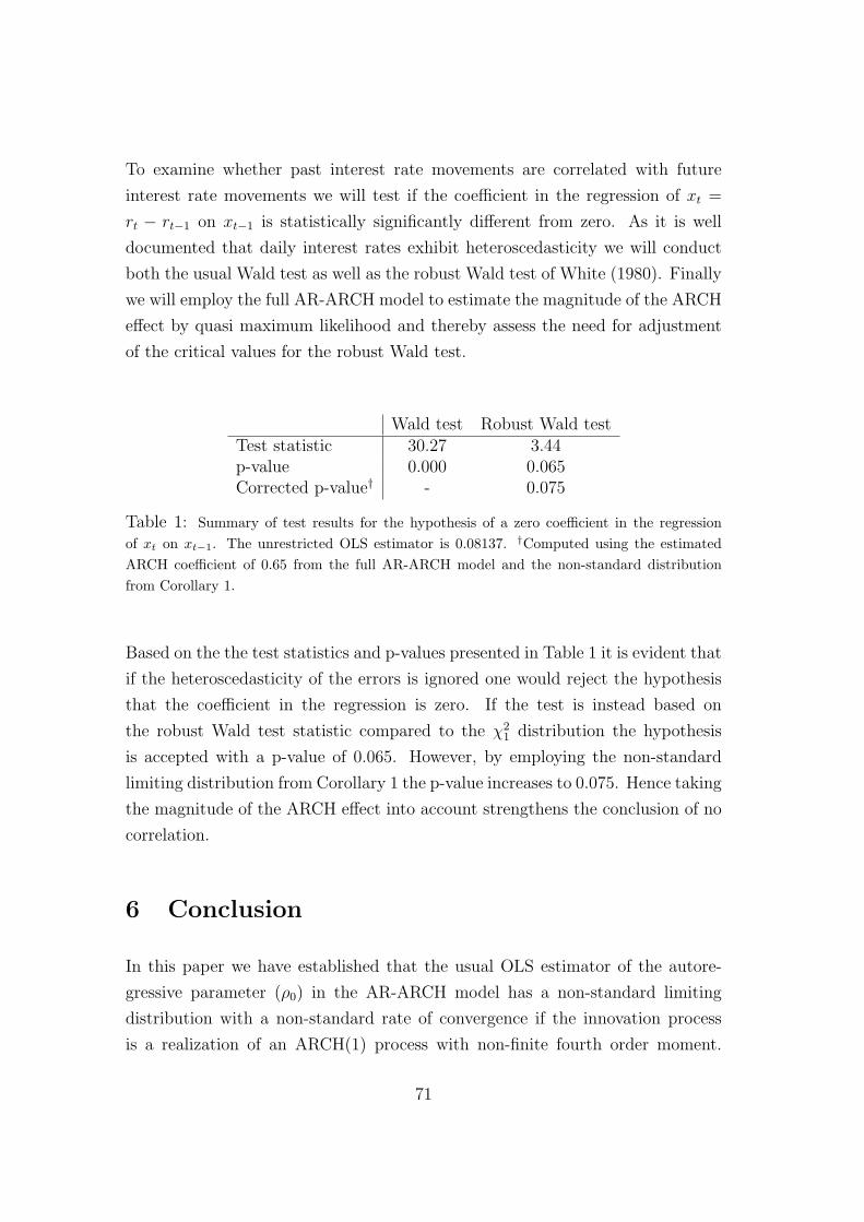
To examine whether past interest rate movements are correlated with future
interest rate movements we will test if the coefficient in the regression of xt =
rt − rt−1 on xt−1 is statistically significantly different from zero. As it is well
documented that daily interest rates exhibit heteroscedasticity we will conduct
both the usual Wald test as well as the robust Wald test of White (1980). Finally
we will employ the full AR-ARCH model to estimate the magnitude of the ARCH
effect by quasi maximum likelihood and thereby assess the need for adjustment
of the critical values for the robust Wald test.
Wald test Robust Wald testTest statistic 30.27 3.44p-value 0.000 0.065Corrected p-value† - 0.075
Table 1: Summary of test results for the hypothesis of a zero coefficient in the regressionof xt on xt−1. The unrestricted OLS estimator is 0.08137. †Computed using the estimatedARCH coefficient of 0.65 from the full AR-ARCH model and the non-standard distributionfrom Corollary 1.
Based on the the test statistics and p-values presented in Table 1 it is evident that
if the heteroscedasticity of the errors is ignored one would reject the hypothesis
that the coefficient in the regression is zero. If the test is instead based on
the robust Wald test statistic compared to the χ21 distribution the hypothesis
is accepted with a p-value of 0.065. However, by employing the non-standard
limiting distribution from Corollary 1 the p-value increases to 0.075. Hence taking
the magnitude of the ARCH effect into account strengthens the conclusion of no
correlation.
6 Conclusion
In this paper we have established that the usual OLS estimator of the autore-
gressive parameter (ρ0) in the AR-ARCH model has a non-standard limiting
distribution with a non-standard rate of convergence if the innovation process
is a realization of an ARCH(1) process with non-finite fourth order moment.
71

Furthermore, we have established that the robust t- and Wald test statistics of
White (1980) for the hypothesis ρ0 = 0 have the correct normalization, but a non-
standard limiting distribution when the innovations have non-finite fourth order
moment. The critical values for the non-standard limiting distribution are higher
than the usual N(0,1) and χ21 critical values, respectively, which implies that an
acceptance of the hypothesis using the standard robust t- or Wald tests remains
valid even in the fourth order moment condition is not met. However, the size of
the test might be higher than the nominal size. Hence the analysis presented in
this paper extends the usability of the robust t− and Wald tests of White (1980).
Finally, a small empirical study shows how employing the corrected critical values
can strengthen the evidence of no correlation between consecutive movements of
interest rates.
Appendix
Proof of Theorem 1. Note first that since we have assumed finite fourth and
hence second order moment, yt has the stationary representation y∗t =∑∞
t=0 ρiεt−i,
which will be used when calculating expected values under the stationary distrib-
ution. The second order moments of the ARCH process and the volatility process
are given by
E[ε2t ] = E[ht] =
ω0
1− α0
.
Next the fourth order moment can be derived from
E[ε4t ] = E[z4
t h2t ] = κ(ω2
0 + α20E[ε4
t−1] + 2ω0α0E[ε2t−1]).
Since the expectation is taken with respect to the stationary distribution it holds
that
E[ε4t ] = κ
ω20 + 2ω2
0α0
1−α0
1− κα20
= κω2
0(1 + α0)
(1− κα20)(1− α0)
,
and E[h2t ] = ω2
0(1 + α0)(1 − κα20)−1(1 − α0)
−1. Utilizing the representation for
ht as a function of zt, ..., zt−k and ht−k from Nelson (1990) it holds that for some
72

k ∈ N0
E[ε2t−kε
2t ] = E
[ε2
t−kz2t
(ht−k
k∏i=1
α0z2t−i + ω0
(1 +
k−1∑
k=1
k∏i=1
α0z2t−i
))]
= κE[αk0h
2t−k] + ω0E
[ε2
t−k
1− αk0
1− α0
]
= καk0ω
20
1 + α0
(1− κα20)(1− α0)
+ ω20
1− αk0
(1− α0)2
=ω2
0
(1− α0)2+
ω20α
k0(κ− 1)
(1− κα20)(1− α0)2
.
Using the symmetry of zt’s distribution and the infinite representation of yt yields
E[y2t−1ht] = E
( ∞∑i=0
ρi0εt−1−i
)2
(ω0 + α0ε2t−1)
= ω0
∞∑i=0
ρ2i0 E[ε2
t−i−1] + α0
∞∑i=0
ρ2i0 E[ε2
t−hε2t ]
=ω2
0
(1− α0)(1− ρ20)
+α0ω
20
(1− α0)2(1− ρ20)
+ω2
0α20(κ− 1)
(1− κα20)(1− α0)2
∞∑i=0
αi0ρ
2i0
=ω2
0
(1− α20)(1− ρ2
0)+
ω0(κ− 1)
(1− κα20)(1− α0)2(1− α0ρ2
0),
and
E[y2t−1] = E
( ∞∑i=0
ρi0εt−1−i
)2 =
ω0
(1− α0)(1− ρ20)
.
In order to apply a standard CLT for martingale difference sequences (e.g. Brown
(1971)) we first verify the Lindeberg condition
1
T
T∑t=1
E[y2t−1ε
2t 1|yt−1εt|>δ
√T] ≤
1
δξT 1+ξ/2
T∑t=1
E[(yt−1εt)2+ξ] → 0,
where ξ > 0 is chosen such that the expectation is finite. The constant ξ ex-
ists because the inequality which ensures finite fourth order moment is a sharp
73
inequality, see Lange et al. (2007) for details. Furthermore
1
T
T∑t=1
E[y2t−1ε
2t | Ft−1] =
1
T
T∑t=1
y2t−1ht
P→ E[y2t−1ht].
Hence
√T (ρOLS − ρ0)
D→ N(0, Σ) as T →∞,
where
Σ =(1− α0)
2(1− ρ20)
2
ω20
E[y2t−1ht] = (1− ρ2
0) +(κ− 1)(1− ρ2
0)2α0
(1− κα20)(1− α0ρ2
0).
This completes the proof.
The proof of the Theorem 2 rests to a large extent on the following lemma.
Lemma 2. Under the assumptions of Theorem 2 all finite dimensional vectors
yt(k) = (yt, ..., yt+k) have regularly varying tails as defined in Resnick (1987) with
the same tail index λ as the ARCH process.
Since the process yt clearly has moments of the same order as the ARCH process
this result is by no means surprising. The proof is inspired by the proofs of
Lemma A.3.26 in Embrechts, Kluppelberg & Mikosch (1997) and Lemma 4.24 in
Resnick (1987). However none of these results are directly applicable since the
innovations are not independent.
Proof of Lemma 2. We begin by showing a tamer result, namely that yt is reg-
ularly varying with tail index λ. Since regular variation is a property of the
marginal distribution, the subscript on yt will be omitted.
Since the ARCH process has finite second order moment y has the representation
y =∑∞
i=0 ρiε−i. Define
ym =m∑
i=0
ρiε−i and y′m = y − ym,
74
for some m ≥ 1. We will now show that y′m has negligible influence on the tails
of y for m sufficiently large. Observe that for δ ∈]0, 1[ and some x > 0,
P (ym > x(1 + δ))− P
( ∞∑i=m+1
ρiε−i ≥ δx
)(8)
≤ P (ym > x(1 + δ))− P (y′m ≤ −δx)
≤ P (ym > x(1 + δ), y′m > −δx)
≤ P (y > x)
≤ P (ym > x(1− δ)) + P (y′m > δx)
≤ P (ym > x(1− δ)) + P
( ∞∑i=m+1
ρiε−i ≥ δx
). (9)
In the following we show
limm→∞
lim supx→∞
P (∑∞
i=m |ρ|i|ε−i| > x)
P (|ym| > x)= 0. (10)
Rewrite as
P
( ∞∑i=m
|ρ|iε−i > x
)
= P
( ∞∑i=m
|ρ|iε−i > x,
∞∨i=m
|ρ|i|ε−i| > x
)
+P
( ∞∑i=m
|ρ|iε−i > x,
∞∨i=m
|ρ|i|ε−i| ≤ x
)
≤ P
( ∞⋃i=m
(|ρ|i|ε−i| > x))
+P
( ∞∑i=m
|ρ|i|ε−i|1|ρ|i|ε−i|≤x > x,
∞∨i=m
|ρ|i|ε−i| ≤ x
)
≤∞∑
i=m
P (|ε−i| > x|ρ|−i) + P
( ∞∑i=m
|ρ|i|ε−i|1|ρ|i|ε−i|≤x > x
).
The structure of the model yields the relation P (|ym| > x) ≥ P (|ε0| > 2x), using
75

this and Markov’s inequality in combination with the above give
P (∑∞
i=m |ρ|i|ε−i| > x)
P (|ym| > x)
≤ P (∑∞
i=m |ρ|i|ε−i| > x)
P (|ε0| > 2x)
=P (|ε0| > x)
P (|ε0| > 2x)× P (
∑∞i=m |ρ|i|ε−i| > x)
P (|ε0| > x)
≤ g(x)
( ∞∑i=m
P (|ε−i| > x|ρ|−i)
P (|ε0| > x)+ x−1
∞∑i=m
|ρ|iE[|ε0|1|ε0|≤x|ρ|−i]
P (|ε0| > x)
)
= g(x)(I + II). (11)
By Basrak, Davis & Mikosch (2002b) ε0 has regular varying tails and hence will
g(x) converge toward 2λ. Furthermore for I Proposition 0.8(ii) of Resnick (1987)
implies that there for all τ > 0 exists a x0 such that for all x > x0
P (|ε0| > x|ρ|−i)/P (|ε0| > x) ≤ (1 + τ)|ρ|iτ .
This bound is summable and hence by dominated convergence and the regular
variation of ε0 it holds that lim supx→∞ I ≤ ∑∞i=m |ρ|iλ. In considering II, sup-
pose temporarily that 0 < λ < 1 (this will never be the case when E[ε20] < ∞,
but it is a necessary steep towards proving the full result). From an integration
by parts
E[|ε0|1|ε0|≤x]xP (|ε0| > x)
=
∫ x
0P (|ε0| > u)du
xP (|ε0| > x)− 1
and applying Karamata’s Theorem (from e.g. Resnick (1987)) this converges, to
(1− λ)−1 − 1 = λ(1− λ)−1, as x →∞.
Thus E[|ε0|1|ε0|≤x|ρ|−i] is a regular varying function with tail index 1 − λ and
applying again Proposition 0.8(ii) we have for x sufficiently large and some con-
76

stants k > 0 and 0 < τ < 1
|ρ|iE[|ε0|1|ε0|≤x|ρ|−i]
xP (|ε0| > x)= |ρ|i
(E[|ε0|1|ε0|≤x|ρ|−i]
E[|ε0|1|ε0|≤x]
)E[|ε0|1|ε0|≤x]xP (|ε0| > x)
≤ k|ρ|i(|ρ|−i)1−τ = k|ρ|iτ ,
which is summable. So we conclude
lim supx→∞
II ≤ k
∞∑i=m
|ρ|i|ρ|i(λ−1) = k
∞∑i=m
|ρ|iλ
and hence when 0 < λ < 1 for some k′ > 0
lim supx→∞
P (∑∞
i=m |ρ|i|ε−i| > x)
P (|ym| > x)≤ k′
∞∑i=m
|ρ|iλ < ∞. (12)
If λ ≥ 1 we get a similar inequality by reducing to the case 0 < λ < 1 as
follows. Pick η ∈]λ, λτ−1[ and set c =∑∞
i=m |ρ|i and pi = |ρ|i/c then by Jensen’s
inequality (e.g. Feller (1971) p. 153) we get
( ∞∑i=m
|ρ|i|ε−i|)η
= cη
( ∞∑i=m
pi|ε−i|)η
≤ cη
∞∑i=m
pi|ε−i|η = cη−1
∞∑i=m
|ρ|i|ε−i|η.
Thus
P (∑∞
i=m |ρ|i|ε−i| > x)
P (|ε0| > x)≤ P (
∑∞i=m |ρ|i|ε−i|η > c1−ηxη)
P (|ε0|η > xη).
By Bingham, Goldie & Teugels (1987) Proposition 1.5.7(i) the function P (|ε0|η >
x) is regularly varying with tail index η−1λ ∈]0, 1[. Hence (12) gives
lim supx→∞
P (∑∞
i=m |ρ|i|ε−i| > x)
P (|ym| > x)≤ k′
∞∑i=m
|ρ|iλη−1
cλ(1−η−1) < ∞. (13)
This proves (10).
77

Combine (8) and (9) with the above to obtain the double inequality
limm→∞
lim supx→∞
P (ym > x(1 + δ))
P (ym > x)≤ lim
m→∞lim sup
x→∞
P (y > x)
P (ym > x)
≤ limm→∞
lim supx→∞
P (ym > x(1− δ))
P (ym > x).
By Basrak et al. (2002b) equation (2.6) ym is regular varying with index λ and
hence will
(1 + δ)−λ ≤ limm→∞
lim supx→∞
P (y > x)
P (ym > x)≤ (1− δ)−λ.
Now by letting δ go towards zero it can be concluded that y is regular varying
with index λ.
Finally we wish to extent this result to all vectors of the form y(k) = (y0, ..., yk).
By Basrak, Davis & Mikosch (2002a) Theorem 1.1(ii) it suffices to show that all
linear combinations v ∈ Rk \ 0 are regular varying. However, for all v
v′y(k) =∞∑i=0
ciε−i,
where the coefficients are absolutely summable and smaller than one in absolute
value for i sufficiently large. Hence can regular variation of y(k) be verified by
the same arguments as above. This completes the proof of Lemma 2
Proof of Theorem 2. Define the empirical autocovariance and the empirical au-
tocorrelation as
γT (r) =1
T
T∑t=1
ytyt+r, r = 0, 1
ρT (1) = γT (1)/γT (0).
These are clearly closely related to the OLS estimator of the autoregressive pa-
rameter. We will therefore in the following prove that γT (r) − E[γT (r)] and
ρT (1)− E[γT (1)]/E[γT (0)] are both asymptotically stable with index λ/2.
Define yt(k) = (yt, ..., yt+k)′ and let aT be a sequence such that TP (|yt| > aT ) → 1
78

(one can choose aT to be the 1−1/T quantile of the distribution function for |yt|).The proof is structured as the proof of Theorem 2.10 in Basrak et al. (2002b),
and we must therefore verify that
(A.1) yt(k) is regularly varying for all k ≥ 1,
(A.2) the mild mixing condition A(aT ) from Davis & Mikosch (1998) p. 2052,
(A.3) condition (2.10) of Davis & Mikosch (1998), and
(A.4) condition (3.3) of Davis & Mikosch (1998) both stated below.
(A.1) follows straight from Lemma 2. Furthermore Lemma 1 establishes that the
Markov chain (yt−1, εt)′ is geometrically ergodic, this implies in particular that the
stationary version is strongly mixing (actually even β-mixing) with geometrically
decreasing rate function. And since the condition A(aT ) is implied by strong
mixing the verification of (A.2) is complete.
The two remaining conditions require a bit more work. Interpreting | · | as the
max norm condition (2.10) of Davis & Mikosch (1998) can be stated as
limm→∞
lim supT→∞
P( ∨
m≤|t|≤rT
|yt(k)| > aT x∣∣|y0(k)| > aT x
)= 0, x > 0, (14)
where rT is an integer sequence such that rT → ∞ as T → ∞. By the defin-
ition of conditional probabilities, Markov’s inequality, and the symmetry of the
distributions it holds that
P (|yt| > aT x | |y0| > aT x) ≤ E[1|y0|2>a2T x2|yt|2]
a2T x2P (|y0|2 > a2
T x2)
=E
[1|y0|2>a2
T x2(ρ2t|y0|2 +
∑t−1i=0 ρ2iε2
t−i)]
a2T x2P (|y0|2 > a2
T x2)=: It,T .
The recursion of Nelson (1990) gives
E0[ε2t ] = h0α
t + ω1− αt
1− α≤ h0α
t + C1,
79
for some positive constant C1 independent of t. Direct calculations yield the
relation
t−1∑i=0
ρ2iαt−i =
α(ρ2t−αt)
ρ2−αif α 6= ρ2
tαt if α = ρ2.
Note that the sum converges to zero as t tends to infinity for all ρ, α smaller
than one in absolute value. Hence by Karamata’s Theorem (e.g. Resnick (1987)
Proposition 0.6) and the equivalent tail behavior of y0 and ε0 it can concluded
that
lim supT→∞
It,T ≤ lim supT→∞
E[1|y0|>aT x
(ρ2t|y0|2 + ε2
0α(ρ2t−αt)
ρ2−α+ C2
)]
a2T x2P (|y0| > aT x)
= C3ρ2t + C4
α(ρ2t − αt)
ρ2 − α
≤ C5at,
for some positive constants C2, ..., C5 and a ∈]0, 1[ all independent of t, since by
assumption both ρ and α are smaller that one in absolute value. Note that the
special case α = ρ2 can be treated using the same arguments. We are now ready
to verify (14).
limm→∞
lim supT→∞
P( ∨
m≤|t|≤rT
|yt(k)| > aT x∣∣|y0(0)| > aT x
)
≤ limm→∞
lim supT→∞
2(k + 1)
rT +k∑t=m
P (|yt| > aT x | |y0| > aT x)P (|y0| > aT x)
P (|y0(k)| > aT x)︸ ︷︷ ︸≤1
≤ limm→∞
2(k + 1)∞∑
t=m
C5at
= 0.
This completes the verification of (A.3). Finally (A.4) is considered. In the setup
80

of the AR-ARCH model condition (3.3) of Davis & Mikosch (1998) reads
limx→0
lim supT→∞
P(∣∣a−2
T
T∑t=1
ytyt+11|ytyt−1|≤a2T x − E
[a−2
T
T∑t=1
ytyt+11|ytyt−1|≤a2T x
]∣∣ > δ)
= 0,
for all δ > 0, which can also be found in Davis & Hsing (1995) p. 895. Markov’s
inequality and Kamarata’s Theorem now give
P
(∣∣∣∣∣a−2T
T∑t=1
ytyt+11|ytyt−1|≤a2T x − E
[a−2
T
T∑t=1
ytyt+11|ytyt−1|≤a2T x
]∣∣∣∣∣ > δ
)
≤ 2
δE
[∣∣∣∣∣a−2T
T∑t=1
ytyt+11|ytyt−1|≤a2T x
∣∣∣∣∣
]
≤ 2T
a2T δ
E[|ytyt+1|1|ytyt−1|≤a2
T x]
∼ C6xTP (|ytyt+1| > a2T x)
→ C7x as T →∞→ 0 as x → 0.
Using the same arguments, it can be shown that (A.4) also holds for the sequence
y2t instead of ytyt+1. This completes the verification of (A.4). Due to (A.1) to
(A.4) one can apply Theorem 3.5, of Davis & Mikosch (1998). Note that their
condition (3.4) is not meet, but by inspecting the proof it becomes clear that
(A.4) suffices. Hence it holds that
Ta−2T (γT (r)− E[γT (r)])
D→ Vr as T →∞, r = 0, 1
Ta−2T (ρT (1)− E[γT (1)]/E[γT (0)])
D→ S0 as T →∞,
where V0, V1, and S0 are λ/2-stable random variables. Since aT can be chosen to
be the 1 − 1/T quantile of the distribution function of |yt|, which tail behaves
like |yt|−λ, one gets that aT can be chosen as aT = T 1/λ. This implies that the
normalizing sequence Ta2T can be chosen as T 1−2/λ Hence it holds that
T 1−2/λ(ρOLS − ρ0) = T 1−2/λ(ρT (1)− E[γT (1)]/E[γT (0)])D→ S0.
81
This completes the proof.
Proof of Theorem 3. Since the process (εt)Tt=1 is an ARCH(1) process it follows
directly from Davis & Mikosch (1998) pp. 2069 - 2070 that
T−2/λ
T∑t=1
εtεt−1D→ S1 and T−4/λ
T∑t=1
ε2t ε
2t−1
D→ S2,
where the vector (S1, S2) is jointly a λ/2 stable random variable, with the remain-
ing parameters and dependence structure unknown. Under H0 we can rewrite VT
as
VT =(T−2/λ
T∑t=1
εtεt−1
)(T−4/λ
T∑t=1
ε2t ε
2t−1
)−1/2,
and the continuous mapping theorem completes the proof.
82

83

84

On IGARCH and convergence of the QMLEfor misspecified GARCH models
By Anders Tolver Jensen & Theis Lange
Department of Natural Sciences & Department of Mathematical Sciences
University of Copenhagen
E-mail: [email protected] & [email protected]
Abstract: We address the IGARCH puzzle by which we understand the fact that aGARCH(1,1) model fitted by quasi maximum likelihood estimation to virtually anyfinancial dataset exhibit the property that α + β is close to one. We prove that ifdata is generated by certain types of continuous time stochastic volatility models, butfitted to a GARCH(1,1) model one gets that α + β tends to one in probability asthe sampling frequency is increased. Hence, the paper suggests that the IGARCHeffect could be caused by misspecification. The result establishes that the stochasticsequence of QMLEs do indeed behave as the deterministic parameters considered inthe literature on filtering based on misspecified ARCH models, see e.g. Nelson (1992).An included study of simulations and empirical high frequency data is found to be invery good accordance with the mathematical results.
Keywords: GARCH; Integrated GARCH; Misspecification; High frequency exchange
rates.
1 Introduction
A complete characterization of the volatility of financial assets has long been one
of the main goals of financial econometrics. Since the seminal papers of Engle
(1982) and Bollerslev (1986) the class of generalized autoregressive heteroskedas-
tic (GARCH) models has been a key tool when modeling time dependent volatil-
ity. Indeed the GARCH(1,1) model has become so widely used that it is often
referred to as “the workhorse of the industry” (Lee & Hansen 1994).
Recall that given a sequence of returns (yt)t=0,...,T the GARCH(1,1) model defines
the conditional volatility as
σ2t (θ) = ω + αy2
t−1 + βσ2t−1(θ), (1)
85
for some non-negative parameters θ = (ω, α, β)′. Quasi maximum likelihood
estimation of GARCH(1,1) models on financial returns almost always indicates
that α is small, β is close to unity, and the sum of α and β is very close to
one and approaches one as the sample is increased, see e.g. Engle & Bollerslev
(1986), Bollerslev & Engle (1993), Baillie, Bollerslev & Mikkelsen (1996), Ding
& Granger (1996), Andersen & Bollerslev (1997), and Engle & Patton (2001).
This feature seems to be present independently of the considered asset class or
sampling frequency. Engle & Bollerslev (1986) proposed the integrated GARCH
(IGARCH) model specifically to reflect this fact. Also in the recent litterateur on
quasi maximum likelihood estimation in GARCH models it has been paramount
to allow for α + β to be close to or even exceeding one, see e.g. Jensen &
Rahbek (2004a) and Francq & Zakoıan (2004). IGARCH implies that the return
series is not covariance stationary and multiperiod forecasts of volatility will
trend upwards. Recently it has been suggested that either long memory, see e.g.
Mikosch & Starica (2004), or parameter changes, see e.g. Hillebrand (2005), in
the data generating process can give the impression of IGARCH.
In a series of seminal papers Nelson (1992), Nelson & Foster (1994), and Nel-
son & Foster (1995) explore the consequences of applying ARCH type filters on
discrete samples from continuous time stochastic volatility models. One impor-
tant result demonstrates the existence of a deterministic sequence of parameters
for the GARCH(1,1) model such that the difference between the GARCH condi-
tional volatility estimates based on (1) and the true volatility converges to zero in
probability as the sampling frequency is increased. This may explain the success
of ARCH type models at recovering and forecasting volatility even though they
are, no doubt, misspecified. The result, however, depends on the fact that the
chosen parameters have the IGARCH property and do not depend on the data.
Indeed Nelson & Foster (1994) stress the need for extending their results to cover
filters based on quasi maximum likelihood estimators (QMLEs) from ARCH type
models. In addition a number of papers (see, e.g. Drost & Nijman (1993), Drost
& Werker (1996), and Francq & Zakoıan (2000)) explore the connection between
continuous time stochastic volatility models and discrete time GARCH models.
They establish a link between parameters of the two classes of models and conse-
quently suggest that one estimates parameters in the continuous time model from
the GARCH estimates. However, Wang (2002) warns against applying statistical
86

inference based on a GARCH model to its continuous time counterpart as this
may lead to erronerous conclusions. The concerns of Nelson & Foster (1995) and
Wang (2002) illustrate the need to understand better the behaviour of QMLEs
for misspecified GARCH models.
In this paper we propose a simple stochastic volatility type model that enables us
to study the statistical properties of the QMLE based on the GARCH(1,1) model
(1). We prove in Theorem 1 that as the sampling frequency is increased certain
data generating processes will spuriously lead to the conclusion of IGARCH. The
employed infill asymptotics has recently been much used in the literature on
realized volatility, see e.g. Andersen, Bollerslev, Diebold & Labys (2003) and
Barndorff-Nielsen & Shephard (2001).
The paper also provides a more intuitive explanation of the IGARCH puzzle
by exposing similarities between the GARCH model and non-parametric estima-
tion of a volatility process, see Starica (2003) for a related study. The GARCH
model provides a filter for computing the present volatility as, roughly speaking,
a weighted average of past squared observations and a constant. Examination of
the weights and the shape of the quasi likelihood function makes it plausible to
believe that the performance of the filter is optimized when α and β sum to one.
Finally, since the theoretical results not only establish that the sum of the
GARCH parameters will tend to one, but also indicate that they will do so
at a polynomial rate, an illustration using high frequency exchange rates as well
as simulated data is provided. The results are found to be in remarkably good
accordance with the theoretical results and furthermore indicates that Theorem 1
is valid for other models than the ones covered by the present proof.
The rest of the paper is organized as follows. Section 2 presents the main result
and explores connections between the GARCH(1,1) model and non-parametric
estimation of volatility. Section 3 illustrates our results by both simulations and
empirical data, while Section 4 concludes and presents ideas for future research.
All technical lemmas are deferred to the Appendix.
87

2 Main Results
Based on a large class of volatility models this section initially provides a more
heuristic explanation of the IGARCH puzzle by exposing similarities between
the GARCH model and non-parametric estimation of a volatility process. In the
second part of the section we present a mathematical setup where these heuristic
arguments can be formalized and we state our main theorem.
2.1 An Intuitive Explanation of the IGARCH Puzzle
Essentially all volatility models for a sequence (yt)t=0,...,T can be captured by the
formulation
yt =√
ft · zt, (2)
where zt is a sequence of zero mean random variables with unit variance and
(ft)t=0,...,T a sequence of stochastic volatilities such that zt is independent of
(ft, yt−1, . . . , y0). Define σ2t (θ) to be the conditional variance process correspond-
ing to the GARCH(1,1) model with parameters θ = (ω, α, β)′
σ2t (θ) = ω + αy2
t−1 + βσ2t−1(θ)
= ω
t−1∑i=0
βi + α
t−1∑i=0
βiy2t−1−i + βtσ2
0, (3)
with σ20 a fixed constant. Consider the usual quasi log-likelihood function
lT (θ) = − 1
T
T∑t=1
(log(σ2t (θ)) +
y2t
σ2t (θ)
) (4)
and note that under the data generating process given by (2) the likelihood
function may be rewritten as
lT (θ) =1
T
T∑t=1
(1− z2t )
ft
σ2t (θ)
− 1
T
T∑t=1
(log(σ2t (θ)) +
ft
σ2t (θ)
). (5)
88
Strictly speaking this is not a likelihood function, but just an objective function
for the GARCH(1,1) model, but the terminology emphasizes the connection to the
literature on estimation of GARCH models. Since the first term has zero mean (if
finite) and the function x 7→ − log(x)−a/x has a unique maximum at x = a, the
decomposition (5) suggests that for a large class of data generating processes it is
plausible that the likelihood function is optimized when the conditional variance
process is close to the true unobserved volatility process ft.
For large values of t the conditional variance process in (3) can be viewed as
a kernel estimator of the unobserved volatility at time t with kernel weights
αβi, i = 0, . . . , t − 1 on past observations y2t−1, . . . , y
20 plus the constant ω
1−β. In
order for this to be an unbiased estimator of the non-constant volatility f on
average over the entire sample one must have∑∞
i=0 αβi = α1−β
≈ 1 and the
constant ω1−β
small. Hence, when considering the conditional variance process,
σ2t (θ), as a non-parametric estimator of the unobserved volatility one must have
α +β ≈ 1 and ω small in order to avoid introducing a systematical bias. Clearly,
the method above is not always the optimal way to match the conditional variance
process, σ2t (θ), with the volatility process, ft. For instance if the data generating
process is in fact the GARCH(1,1) model one should choose θ to be the true
parameter value and hence obtain σ2t (θ) = ft.
2.2 A Mathematical Explanation of the IGARCH Puzzle
In the following we introduce a mathematical framework allowing us to formalize
the considerations above. Clearly, we cannot give unified mathematical proofs
of our results covering all interesting stochastic volatility models. However, the
framework below offers a compromise between flexibility of the model class and
clarity of the formal mathematical arguments. Following Theorem 1 we discuss
possible generalizations.
Let the continuous time process (Su)u∈[0,1] be a solution to the stochastic differ-
ential equation
dSu =√
f(u)dWu, (6)
89
where W is a standard Brownian motion and f is a strictly positive continuous
function on the unit interval. Consider a discrete sample (rt)t=1,...,T of returns
given by
rt = St/T − S(t−1)/T ∼ N(0,
∫ t/T
(t−1)/T
f(u)du).
For large T the distribution of the returns (scaled by√
T ) will resemble the
distribution of a sequence (yt)t=1,...,T generated by
yt =√
f(t/T ) · zt, (7)
where zt is an i.i.d. sequence of zero mean unit variance Gaussian random vari-
ables. By extending the model in (6) to allow for a stochastic volatility process
f the formulation encompasses a number of applied stochastic volatility models.
Thus we claim that results based on (7) will also be relevant for the continuous
time model (6), see Remark 2. Indeed many of the results by D.B. Nelson con-
cerning misspecified ARCH models, see e.g. Nelson (1992), are based on models
of the type captured by (6) and also make use of rescaling increments of discrete
samples from these models.
Consider the sequence of parameters θT = (0, T−d, 1 − T−d)′ and introduce the
stochastic processes
hT (u) = σ2bTuc(θT )
on u ∈ [0, 1], where σt(θ) is given by the GARCH(1,1) recursion (3). Here and
throughout the paper bxc denotes the integer part of x. Further, let D([a, b])
denote the space of cadlag functions on the interval [a, b].
Lemma 1. If E[z8t ] < ∞ then for any d ∈]1/2, 1[ and γ ∈]0, 1] the process
hTP→ f in the uniform norm on D([γ, 1]) as T tends to infinity.
The lemma establishes that there exists a sequence of parameters such that the
conditional variance process associated with the GARCH(1,1) model gets arbi-
trarily close to the unobserved volatility process when the sampling frequency is
increased. The lemma is an analogue to Theorem 3.1 of Nelson (1992), however,
90
our result is given for the uniform norm, but assuming a somewhat simpler data
generating process.
Proof of Lemma 1. Introduce the notation gT (u) := E[hT (u)] for u ∈ [0, 1]. For
γ, η > 0
P( supu∈[γ,1]
|hT (u)− f(u)| > η)
≤ P( supu∈[γ,1]
|hT (u)− gT (u)| > η/2) + P( supu∈[γ,1]
|gT (u)− f(u)| > η/2).
By Lemma 3 in the Appendix the last term converges to zero as T tends to
infinity. To handle the first term note that by Lemma 2 in the Appendix it holds
that
P( supu∈[γ,1]
|hT (u)− gT (u)| > η/2)
= P( maxt=bTγc−1,...,T
|hT (t/T )− gT (t/T )| > η/2)
≤T∑
t=bTγc−1
P(|hT (t/T )− gT (t/T )| > η/2)
≤ Aη−4Tα2T
which converges to zero as T tends to infinity since αT = T−d with d > 1/2. ¤
Before stating our main theorem define the parameter set
Θ = (ω, α, β)′ ∈ R3 | 0 ≤ ω, 0 ≤ α ≤ 1, 0 ≤ β ≤ 1 (8)
and let θT = (ωT , αT , βT )′ = arg maxθ∈Θ lT (θ) be the usual quasi maximum like-
lihood estimator based on (4).
Theorem 1. Suppose that the data generating process is given by (7) where f
is non-constant and E[z8t ] < ∞. Then the QMLE based on (4) satisfies that
(ωT , αT , βT )′P→ (0, 0, 1)′ as T tends to infinity.
Remark 1. The initial value σ20 for the conditional volatility process σ2
t (θ) does
not need to be a constant. For instance Theorem 1 still holds if σ20 is merely
91

bounded in probability as T tends to infinity. This includes defining σ20 as the
unconditional variance of the full sample, which is implemented in many software
packages.
Remark 2. When defining σ20 as the unconditional variance of the full sample
it is a simple consequence of the GARCH(1,1) recursion that any scaling of the
observations only affects the estimate of the scale parameter ω. Hence, if the
QMLE is based on the unscaled returns, rt, from the continuous time model (6)
Theorem 1 remains valid. When extending the model (6) to allow for a stochastic
volatility the present proof of Theorem 1 requires that the volatility process be
independent of the Brownian motion. In this case the result should be read as
conditional on the sample path of the volatility process.
Remark 3. To facilitate the presentation we have assumed that the volatility
process f is a continuous function. However, the proofs can be extended to cover
a finite number of discontinuities at the price of a somewhat more cumbersome
notation and Theorem 1 therefore remains valid.
Remark 4. The proof is given for the case of Gaussian innovations zt, however,
it can easily be adapted to most other distributions such as the t-distribution as
long as the moment condition in Theorem 1 is met. Another generalization is to
allow for some dependence in the sequence of innovations. For instance including
an autoregressive structure on zt would permit modeling leverage effects, but
leads to considerably more complicated proofs.
Proof of Theorem 1. For ωU > 0 divide the full parameter space Θ defined in (8)
into the compact subset
ΘωU:= θ = (α, β, ω)′ ∈ Θ | ω ≤ ωU
and its complement ΘcωU
. Let
Vε(0, 0, 1) = (ω, α, β)′ ∈ Θ | ||(ω, α, β)′ − (0, 0, 1)′|| < ε
and use Lemma 6 in the Appendix to construct a finite covering
∪ki=1V (θi) ⊃ ΘωU
\Vε(0, 0, 1)
of the compact set ΘωU\Vε(0, 0, 1) with open subsets of Θ and let γθ1 , . . . , γθk
> 0
92

be constants such that according to Lemma 6
limT→∞
P( supθ∗∈V (θi)
lT (θ∗) < −∫ 1
0
log(f(u))du− 1− γθi) = 1
for i = 1, . . . , k. With γ = min(γθ1 , . . . , γθk) we conclude that
1 ≥ P( supθ∈Θ\Vε(0,0,1)
lT (θ) < −∫ 1
0
log(f(u))du− 1− γ)
≥ P( supθ∈∪k
i=1V (θi)∪ΘcωU
lT (θ) < −∫ 1
0
log(f(u))du− 1− γ)
≥ 1−k∑
i=1
P( supθ∈V (θi)
lT (θ) ≥ −∫ 1
0
log(f(u))du− 1− γ) (9)
− P( supθ∈Θc
ωU
lT (θ) ≥ −∫ 1
0
log(f(u)))du− 1− γ) (10)
where by construction (9) converges to one as T tends to infinity. Further, as
σ2t (θ) ≥ ωU on Θc
ωUwe get that
supθ∈Θc
ωU
lT (θ) = supθ∈Θc
ωU
− 1
T
T∑t=1
(log(σ2t (θ)) +
y2t
σ2t (θ)
) ≤ − log(ωU)
hence the probability in (10) is zero if we choose ωU large enough. By Lemma 4
in the Appendix it holds that lT (θT )P→ − ∫ 1
0log(f(u))du− 1 and since lT (θT ) ≥
lT (θT ) we conclude that for any ε > 0
limT→∞
P(θT ∈ Vε(0, 0, 1)) = 1.
¤
3 Illustrations
The main result (Theorem 1) establishes that for certain data generating processes
the quasi maximum likelihood estimators for the GARCH(1,1) model will con-
verge to (0, 0, 1)′ as the sampling frequency increases. In this section we illustrate
93

the convergence results and go a step further by examining the rate of conver-
gence as well. Based on Lemma 1 one could conjecture that αT and 1 − βT are
proportional to T−d for some d ∈ (0, 1). This assertion can be visualized by plot-
ting log(αT ) and log(1− βT ) against log(T ). If a linear relationship is found the
parameter d can be estimated by ordinary least squares.
The first part of the study is based on high frequency recordings of the EUR-USD
exchange rate. To increase the empirical relevance of the simulation part we use
broadly applied continuous time models as data generating processes. However,
formally these models do not satisfy the assumptions of Theorem 1. In this
respect the simulation study actually demonstrates that the scope of the results
might be extended to a wider class of models.
EUR-USD. Based on 30-minute recordings of the EUR-USD exchange rate span-
ning the period from the 2nd of February 1986 to the 30th of March 20071 log-
returns are computed corresponding to 4 through 72 hour returns. This gives
estimates θT for T between 3.687 and 64.525.
Simulations. We consider three different simulation setups including the Heston
model and the continuous GARCH model (obtained as the diffusion limit of
a GARCH(1,1) model, see Nelson (1990)). The considered models can all be
embedded in the formulation
dSu = SuV1/2u dW1u, dVu = κV a
u (µ− Vu)du + σV bu dW2u,
where W1 and W2 are standard Brownian motions with a possibly non-zero cor-
relation denoted by ρ. For ease of exposition we have omitted a drift term in the
equation for dSu. We will consider three configurations for the parameters a and
b, corresponding to the Heston model, the continuous GARCH model, and the
3/2N model suggested in Christoffersen, Jacobs & Mimouni (2007). To make the
simulations comparable to the empirical study we consider a fixed time span of
21 years. For the remaining parameters we choose the estimated values stated
in Christoffersen et al. (2007), which are based on fitting the models to S&P-500
data. By this choice of time span and parameter values it is reasonable to com-
1Prior to January 1999 the series is generated from the DEM-USD exchange rate using afixed exchange rate of 1.95583 DEM per EUR. Preceding the analysis the dataset has beencleaned as described in Andersen et al. (2003).
94

Name a b κ µ σ ρHeston 0 1/2 6.5200 0.0352 0.4601 -0.7710Continuous GARCH 0 1 3.9248 0.0408 2.7790 -0.78763/2N 1 3/2 60.1040 0.0837 12.4989 -0.7591
Table 1: Parameter values used in the simulation study.
pare the empirical study and the simulation study directly. GARCH(1,1) models
are fitted to log-returns based on a discrete sample from the S process2. Table 1
summarizes the parameters (per annum) for the included models. We will con-
sider log-returns corresponding to weekly through 5 minute returns, which gives
estimates θT for T between 1,000 and 300,000.
Figure 1 reports the correspondence between the estimates of α and T for the
four setups. The conjectured linear relationship between log(αT ) and log(T ) is
clearly present. The corresponding plots for 1− βT have been omitted since they
are indistinguishable from Figure 1. In particular we have verified the IGARCH
property, i.e. that (αT , βT ) → (0, 1). The estimated values for d are in all cases
found to be between 0.25 and 0.5, but explaining this phenomenon is left for
future research.
The fact that none of the simulations satisfy the assumptions clearly indicates
that Theorem 1 holds for a far larger class of models than those covered by the
present version of our proof. This emphasizes that the IGARCH effect can be
caused by the mathematical structure of a GARCH model alone and hence might
not be a property of the true data generating mechanism. That the apparent
polynomial convergence of the QMLEs is not only a property of the simulated
series is illustrated by the striking similarities between plots based on simulated
and real data.
4 Conclusion
In this paper we have established that when a GARCH(1,1) model is fitted to
a discrete sample from a certain class of continuous time stochastic volatility
models then the sum of the quasi maximum likelihood estimates of α and β will
2The continuous time process is simulated by a standard Euler scheme using 108 data points.
95
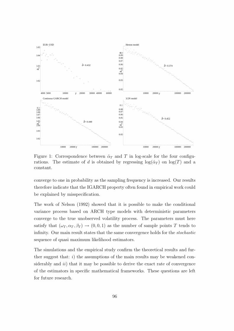
0.02
0.03
0.04
0.05
4000 5000 10000 20000 30000 40000 60000
EUR−USD
α T
T
d= 0.432
0.02
0.03
0.04
0.05
0.06
0.070.080.090.10.1
10000 20000 100000 200000
Heston model
α T
T
d= 0.374
0.02
0.03
0.04
0.05
0.060.070.080.090.1
10000 20000 100000 200000
Continous GARCH model
α T
T
d= 0.440
0.02
0.03
0.04
0.05
0.060.070.08
0.1
10000 20000 100000 200000
3/2N model
α T
T
d= 0.452
Figure 1: Correspondence between αT and T in log-scale for the four configu-rations. The estimate of d is obtained by regressing log(αT ) on log(T ) and aconstant.
converge to one in probability as the sampling frequency is increased. Our results
therefore indicate that the IGARCH property often found in empirical work could
be explained by misspecification.
The work of Nelson (1992) showed that it is possible to make the conditional
variance process based on ARCH type models with deterministic parameters
converge to the true unobserved volatility process. The parameters must here
satisfy that (ωT , αT , βT ) → (0, 0, 1) as the number of sample points T tends to
infinity. Our main result states that the same convergence holds for the stochastic
sequence of quasi maximum likelihood estimators.
The simulations and the empirical study confirm the theoretical results and fur-
ther suggest that: i) the assumptions of the main results may be weakened con-
siderably and ii) that it may be possible to derive the exact rate of convergence
of the estimators in specific mathematical frameworks. These questions are left
for future research.
96

Appendix: Auxiliary lemmas
Lemma 2. If E[z8t ] < ∞ there exists some A > 0 such that for any η > 0
supu∈[0,1]
P[|hT (u)− gT (u)| > η] ≤ Aη−4α2T .
Proof. It follows from Chebychev’s inequality that
P(|hT (u)− gT (u)| > η)
≤ η−4E[|hT (u)− gT (u)|4]
≤ η−4E[(αT
bTuc−1∑t=0
βtT f( bTuc−1−t
T)(z2
bTuc−1−t − 1))4]
≤ η−4||f ||∞α4T
bTuc−1∑t=0
β4tT κ4 + 2η−4α4
T
bTuc−1∑t=1
t−1∑j=0
β2t+2jT κ2
2
≤ A1η−4α4
T (∞∑
t=0
β4tT +
∞∑t=1
β2tT
1−β2tT
1−β2T
),
where we make use of the fact that f is bounded and that κ1 = 0 with kr :=
E[(z2t − 1)r]. Evaluating the geometric series above, using that αT = 1− βT , and
that the last expression does not depend on u one arrives at an inequality of the
form stated in the lemma. ¤
Lemma 3. For any γ > 0 then supu∈[γ,1] |gT (u)−f(u)| → 0 as T tends to infinity.
Proof. For any sequence cT and any u ∈ [γ, 1] we get
|gT (u)− f(u)|
= |βbTucT σ2
0 + αT
bTuc−1∑t=0
βtT (f( bTuc−t−1
T)− f(u))− αT
∞∑
t=bTucβt
T f(u)|
≤ βbTucT σ2
0 + αT
cT−1∑t=0
βtT |f( bTuc−t−1
T)− f(u)|+ αT
∞∑t=cT
βtT ||f ||∞
≤ βbTγcT σ2
0 + αT1− βcT
T
1− βT
supv∈[u− cT
T,u]
|f(v)− f(u)|+ αTβcT
T
1− βT
||f ||∞.
97

If cT /T = o(1) the uniform continuity of f implies that the middle term can be
made arbitrary small by choosing T adequately large and that the convergence
is uniform over u ∈ [γ, 1]. To complete the proof note that
log(βcTT ) = cT log(1− T−d) = −cT T−d log(1− T−d)− log(1)
T−d→ −∞
as T tends to infinity provided that we choose cT so that cT /T d tends to infinity
as T tends to infinity. ¤
Lemma 4. For d > 1/2 then
lT (θT )P→ −
∫ 1
0
log(f(u))du− 1, as T →∞.
Proof of Lemma 4. Rewriting the expression for lT (θT ) yields
lT (θT ) = − 1
T
T∑t=1
(log(σ2t (θT )) +
f(t/T )
σ2t (θT )
) (11)
− 1
T
T∑t=1
f(t/T )
σ2t (θT )
(z2t − 1) (12)
By the law of large numbers for martingale difference sequences (12)P→ 0. For-
mally, since E[z2t − 1] = 0 and σ2
t (θT ) is Ft−1−measurable we get by applying
Chebechev’s inequality that
P(| 1T
T∑t=1
f(t/T )
σ2t (θT )
(z2t − 1)| > η)
≤ B1
T 2
T∑i=1
T∑j=i
E[E[(z2
i − 1)(z2j − 1)
σ2i (θT )σ2
j (θT )| Fj−1]]
=B2
T 2
T∑t=1
E[1
σ4t (θT )
] ≤ B3
Tα2T β2cT
T
E[1
(z21 + . . . + z2
cT)2
],
where cT is a sequence of positive integers. For T sufficiently large (Mathai &
98
Provost (1992), p. 59)
E[1
(z21 + . . . + z2
cT
)2] ≤ B4
c2T
hence
0 ≤ lim supT→∞
P(| 1T
T∑t=1
f(t/T )
σ2t (θT )
(z2t − 1)| > η) ≤ lim sup
T→∞
B5
Tα2T β2cT
T c2T
and by choosing cT = bα−1T c = bT dc the right hand side is zero.
For any γ > 0 (11) may be written as
− 1
T
bTγc−1∑t=1
log(σ2t (θT ))− 1
T
bTγc−1∑t=1
f(t/T )
σ2t (θT )
−∫ 1
γ
log(hT (u))du−∫ 1
γ
f(u)
hT (u)du +
T∑
t=bTγc
∫ t/T
(t−1)/T
f(u)− f(t/T )
hT (u)du,
using that hT (u) is piecewise constant on intervals of the form [(t − 1)/T, t/T [.
We deduce from Theorem 1 and the continuous mapping theorem that
∫ 1
γ
log(hT (u))duP→
∫ 1
γ
log(f(u))du
∫ 1
γ
f(u)
hT (u)du
P→ 1− γ
∫ 1
γ
1
hT (u)du
P→∫ 1
γ
1
f(u)du.
By the uniform continuity of f we conclude that
T∑
t=bTγc
∫ t/T
(t−1)/T
f(u)− f(t/T )
hT (u)du
P→ 0.
99

For η > 0 then
P(| 1T
bTγc−1∑t=1
1
σ2t (θT )
| > η) ≤ P( maxt=1,...,bTγc−1
1
T
1
σ2t (θT )
>η
bTγc − 1)
≤ P( mint=1,...,bTγc−1
σ2t (θT ) ≤ γ
B6
)
≤bTγc∑t=1
P(σ2t (θT ) ≤ γ
B6
).
Noting that E[σ2t (θT )] ≥ min(f, σ2
0) ≡ σ2 > 0 uniformly in t and T we find that
for γ > 0 sufficiently small then
P(σ2t (θ) ≤
γ
B6
) ≤ P(|σ2t (θT )− E[σ2
t (θT )]| ≥ E[σ2t (θT )]− γ
B6
)
≤ P(|σ2t (θT )− E[σ2
t (θT )]| ≥ σ2 − γ
B6
)
we get by applying Lemma 2 that
P(| 1T
bTγc−1∑t=1
1
σ2t (θT )
| > η) ≤ B7bTγcα2T
which tends to zero as T tends to infinity. For η > 0 given we get
P(| 1T
bTγc−1∑t=1
log(σ2t (θT ))| > η)
≤ P( maxt=1,...,bTγc−1
| 1T
log(σ2t (θT ))| > η
bTγc − 1)
≤ P( maxt=1,...,bTγc−1
σ2t (θT ) ≥ exp(B8/γ)) + P( min
t=1,...,bTγc−1σ2
t (θT ) ≤ exp(−B8/γ))
≤bTγc−1∑
t=1
P(σ2t (θT ) ≥ exp(B8/γ)) +
bTγc−1∑t=1
P(σ2t (θT ) ≤ exp(−B8/γ)).
100
From the previous argument we find that for γ > 0 sufficiently small
P(σ2t (θT ) ≥ exp(B8/γ)) ≤ P(|σ2
t (θT )− E[σ2t (θT )]| ≥ exp(B8/γ)− σ2)
P(σ2t (θT ) ≤ exp(−B8/γ)) ≤ P(|σ2
t (θT )− E[σ2t (θT )]| ≥ σ2 − exp(−B8/γ)),
where σ2 = σ20 + ‖f‖∞. From Lemma 2 we get that
P(| 1T
bTγc−1∑t=1
log(σ2t (θT ))| > η) ≤ B9bTγcα2
T
as T tends to infinity. ¤
Lemma 5. For any θ ∈ Θ it holds that if f is non-constant there exists a constant
cθ > 0 such that
limT→∞
P(lT (θ)− −∫ 1
0
log(f(u))du− 1 < −cθ) = 1.
Proof of Lemma 5. Assume initially that θ is such that α 6= 0 and β 6= 0, 1 and
rewrite the log-likelihood function as follows
lT (θ)− −∫ 1
0
log(f(u))du− 1
=
∫ 1
0
log(f(u))du− 1
T
T∑t=1
log(f(t/T ))− 1
T
T∑t=1
f(t/T )
σ2t (θ)
(z2t − 1) (13)
+1
T
T∑t=1
log(f(t/T )
σ2t (θ)
) +σ2
t (θ)− f(t/T )
σ2t (θ)
. (14)
By the LLN for martingale differences (13) tends to zero in probability as T tends
to infinity. Formally, since E[z2t − 1] = 0 and σ2
t (θ) is measurable with respect to
101
Ft−1 = F(z0, ..., zt−1) we get by applying Chebechev’s inequality that
P(| 1T
T∑t=1
f(t/T )
σ2t (θ)
(z2t − 1)| > η)
≤ C1
T 2
T∑i=1
T∑j=i
E[E[(z2
i − 1)(z2j − 1)
σ2i (θ)σ
2j (θ)
| Fj−1]]
=C2
T 2
T∑t=1
E[1
σ4t (θ)
] ≤ C3
TE[
1
(α(z25 + βz2
4 + . . . + β4z21))
2]
and the expectation on the right hand side is finite if α, β > 0 c.f. Mathai &
Provost (1992).
Next turn to the expression in (14) which we decompose into
1
T
T∑t=1
(log(f(t/T )
σ2t (θ)
)− E[log(f(t/T )
σ2t (θ)
)]) (15)
+1
T
T∑t=1
(E[f(t/T )
σ2t (θ)
]− f(t/T )
σ2t (θ)
) (16)
+1
T
T∑t=1
E[log(f(t/T )
σ2t (θ)
) +σ2
t (θ)− f(t/T )
σ2t (θ)
] (17)
Initially we will establish that (15) converges in probability to zero. For any
η > 0 direct calculations yield
P(|T−1
T∑t=1
log(f(t/T )
σ2t (θ)
)− E[log(f(t/T )
σ2t (θ)
)]| > η)
= P(|T−1
T∑t=1
log(σ2t (θ))− E[log(σ2
t (θ))]| > η)
≤ 2
T 2η2
T∑i=1
T∑j=i
|cov(log(σ2i (θ)), log(σ2
j (θ)))|. (18)
102

Utilizing the following inequalities
− 1√x≤ log(x) ≤ √
x, 0 ≤ log(1 + x) ≤ x,
which hold for all strictly positive x, it can be concluded that
|Cov(log(σ2i (θ)), log(σ2
j (θ)))|
= |Cov(log(σ2i (θ)), log(βj−iσ2
i (θ) + ω1− βj−i
1− β+ α
j−i−1∑
k=0
βky2j−1−k
︸ ︷︷ ︸:=Z(i,j)
))|
= |Cov(log(σ2i (θ)), log(Z(i, j)(1 +
βj−iσ2i (θ)
Z(i, j))))|
= |Cov(log(σ2i (θ)), log(1 +
βj−iσ2i (θ)
Z(i, j)))|
≤√E[(log(σ2
i (θ)))2]
√E[(log(1 +
βj−iσ2i (θ)
Z(i, j)))2]
≤√E[(
1√σ2
i (θ)+
√σ2
i (θ))2]
√E[(
βj−iσ2i (θ)
Z(i, j))2]
≤ βj−i
√E[(σ2
i (θ) +1
σ2i (θ)
+ 2)]√E[σ4
i (θ)]
√E[
1
Z(i, j)2].
For j > i + 1 the right hand side can be bounded by βj−1C4, where the constant
C4 does not depend on either i nor j. In the derivations it is used repeatedly
that σ2i (θ) is independent of Z(i, j). Since T−2
∑Ti=1
∑Tj=i β
j−i tends to zero as T
tends to infinity it can be concluded that (18) and hence also (15) tends to zero.
103
To show that (16) tends to zero in probability note that
|Cov(f(i/T )
σ2i (θ)
,f(j/T )
σ2j (θ)
)|
= |f(i
T)f(
j
T)(E[
1
σ2i (θ)
1
βj−iσ2i (θ) + Z(i, j)
]− E[1
σ2i (θ)
]E[1
βj−iσ2i (θ) + Z(i, j)
])|
≤ f(i
T)f(
j
T)E[
1
σ2i (θ)
] | E[1
Z(i, j)]− E[
1
βj−iσ2i (θ) + Z(i, j)
]|
≤ f(i
T)f(
j
T)E[
1
σ2i (θ)
]E[βj−iσ2
i (θ)
Z(i, j)(βj−iσ2i (θ) + Z(i, j))
]
≤ βj−if(i
T)f(
j
T)E[
1
σ2i (θ)
]E[σ2i (θ)]E[
1
Z(i, j)2].
As before if j > i + 4 the expression can be bounded by βj−1C5, where the
constant C5 does not depend on either i nor j. Hence it can be concluded that
(16) tends to zero. Before turning towards (17) note that for any η > 0 it holds
that
P(σ2t (θ) /∈ [f − η, ‖f‖∞ + η]) ≥ P(σ2
t (θ) > ‖f‖∞ + η)
≥ P(αfz2t > ‖f‖∞ + η) = C6 > 0.
Furthermore since the function x 7→ log(a/x)+ (x−a)/x has a unique maximum
at a with the value 0 and the function f is strictly positive and bounded there
exists a constant C7 > 0 such that
supa∈[f,‖f‖∞]
supx∈[0,a−η]∪[a+η,∞]
log(a/x) + (x− a)/x < −C7.
104

Finally it can be concluded that (17) can be bounded by
1
T
T∑t=1
E[log(f(t/T )
σ2t (θ)
) +σ2
t (θ)− f(t/T )
σ2t (θ)
]
≤ 1
T
T∑t=1
−C7P(σ2t (θ) /∈ [f − η, ‖f‖∞ + η])
≤ 1
T
T∑t=1
−C7C6 = −C7C6 = cθ < 0,
which verifies the claim of the lemma. For the special cases α = 0 or β = 0
the lemma is trivially satisfied. If β = 1 the lemma follows from observing σ2t (θ)
tends to infinity almost surely as t grows. ¤
Lemma 6. For θ ∈ Θ\(0, 0, 1) there exists an open subset of Θ around θ denoted
V (θ) and a constant γθ > 0 such that
P( supθ∗∈V (θ)
lT (θ∗) < −∫ 1
0
log(f(u))du− 1− γθ)
tends to one as T tends to infinity.
Proof of Lemma 6. We divide the proof into seven cases mainly because we have
to be very careful when θ lies on the boundary of Θ.
1. θ = (ω, α, β)′ ∈ (0,∞)× [0, 1]× [0, 1)
2. θ = (ω, α, β)′ ∈ (0,∞)× (0, 1]× 1
3. θ = (ω, α, β)′ ∈ (0,∞)× 0 × 1
4. θ = (ω, α, β)′ ∈ 0 × (0, 1]× 0
5. θ = (ω, α, β)′ ∈ 0 × (0, 1]× (0, 1)
6. θ = (ω, α, β)′ ∈ 0 × (0, 1]× 1
7. θ = (ω, α, β)′ ∈ 0 × 0 × [0, 1)
105

Case 1. Choose according to Lemma 5 a cθ > 0 such that
limT→∞
P(lT (θ)− −∫ 1
0
log(f(u))du− 1 ≥ −cθ) = 0.
For ε > 0 denote by
Vε(θ) = θ∗ ∈ Θ | ||θ∗ − θ|| ≤ ε
and note that for T sufficiently large
P( supθ∗∈Vε(θ)
lT (θ∗) < −∫ 1
0
log(f(u))du− 1− cθ/2)
= 1− P( supθ∗∈Vε(θ)
lT (θ) ≥ −∫ 1
0
log(f(u))du− 1− cθ/2)
≥ 1− P(lT (θ) ≥ −∫ 1
0
log(f(u))du− 1− cθ)− P( supθ∗∈Vε(θ)
|lT (θ∗)− lT (θ)| ≥ cθ/2).
To complete the proof we only need to show that for some sufficiently small ε > 0
then
limT→∞
P( supθ∗∈Vε(θ)
|lT (θ∗)− lT (θ)| ≥ cθ/2) = 0. (19)
Note that this is much weaker than proving that
supθ∗∈Vε(θ)
|lT (θ∗)− lT (θ)|
converges to zero in probability since the probability in (19) should not necessarily
converge to zero for this particular ε if cθ is replaced by an arbitrarily small
positive number. We proceed by showing that there exists a constant, D1 > 0,
such that for any small ε > 0 then
supθ∗∈Vε(θ)
|lT (θ∗)− lT (θ)|
can be bounded above by something that converges in probability to D1ε as T
tends to infinity. In particular, the conclusion given by (19) holds for ε > 0 such
106

that D1ε < cθ/2.
Trivially, for ε sufficiently small we get the inequalities
supθ∗∈Vε(θ)
|βt − β∗t| ≤ εt(β + ε)t−1
supθ∗∈Vε(θ)
|αβt − α∗β∗t| ≤ εαt(β + ε)t−1 + ε(β + ε)t
supθ∗∈Vε(θ)
|ωt−1∑i=0
βi − ω∗t−1∑i=0
β∗i| ≤ ε1
1− β+ ε(ω + ε)
∞∑i=0
i(β + ε)i−1.
Hence
supθ∗∈Vε(θ)
|σ2t (θ)− σ2
t (θ∗)|
≤ D1ε + ||f ||∞ε
t−1∑i=0
z2t−1−i [αi(β + ε)i−1 + (β + ε)i]︸ ︷︷ ︸
:=ci
+εt(β + ε)t−1σ20 (20)
and
supθ∗∈Vε(θ)
1
T
T∑t=1
|σ2t (θ)− σ2
t (θ∗)|
≤ 1
T
T∑t=1
supθ∗∈Vε(θ)
|σ2t (θ)− σ2
t (θ∗)|
≤ D1ε + ||f ||∞ε
T∑t=1
t−1∑i=0
z2t−1−ici +
1
T
T∑t=1
t(β + ε)t−1σ20ε
≤ D2ε + ||f ||∞ε∞∑i=0
ci 1
T
T−1∑t=0
z2t
P→ D3ε
as T tends to infinity. As σ2t (θ
∗) is bounded below by ω−ε on Vε(θ) the derivations
just above demonstrate that
supθ∗∈Vε(θ)
1
T
T∑t=1
| log(σ2t (θ))− log(σ2
t (θ∗))| ≤ sup
θ∗∈Vε(θ)
1
T
T∑t=1
1
ω − ε|σ2
t (θ)− σ2t (θ
∗)|
107

is bounded above by something that converges in probability to D4ε as T tends
to infinity. Consider now the decomposition
supθ∗∈Vε(θ)
|lT (θ)− lT (θ∗)|
≤ supθ∗∈Vε(θ)
1
T
T∑t=1
| log(σ2t (θ))− log(σ2
t (θ∗))|
+ ||f ||∞ 1
T
T∑t=1
z2t sup
θ∗∈Vε(θ)
| 1
σ2t (θ)
− 1
σ2t (θ
∗)|
≤ supθ∗∈Vε(θ)
1
T
T∑t=1
1
ω − ε|σ2
t (θ)− σ2t (θ
∗)| (21)
+||f ||∞
(ω − ε)2
1
T
T∑t=1
(z2t − 1) sup
θ∗∈Vε(θ)
|σ2t (θ)− σ2
t (θ∗)| (22)
+||f ||∞
(ω − ε)2
1
T
T∑t=1
supθ∗∈Vε(θ)
|σ2t (θ)− σ2
t (θ∗)|. (23)
It follows by previous computations that (21) and (23) can be bounded above by
variables converging in probability to constants of the form Dε. The remaining
term (22) is a martingale difference and by (20) we find that for ε > 0 sufficiently
small
0 ≤ supθ∗∈Vε(θ)
|σ2t (θ)− σ2
t (θ∗)|
≤ D5ε + D6εt−1∑i=0
(z2t−1−i − 1)ci.
108
This implies that
E[(1
T
T∑t=1
(z2t − 1) sup
θ∗∈Vε(θ)
|σ2t (θ)− σ2
t (θ∗)|)2]
≤ κ22
1
T 2
T∑t=1
E[( supθ∗∈Vε(θ)
|σ2t (θ)− σ2
t (θ∗)|)2]
≤ 1
TD2
5ε2 + D2
6ε2 1
T 2
T∑t=1
E[(z21 − 1)2]
t−1∑i=0
c2i
≤ 1
TD2
5ε2 +
1
TD2
6ε2κ2
∞∑i=0
c2i
verifying that (22) tends to zero in probability which is much stronger that what
we need.
Case 2 and 6. Note initially that for ε adequately small
infθ∗∈Vε(θ)
σ2t (θ
∗) ≥ (α− ε)t−1∑i=0
(1− ε)ifz2t−1−i ≡ σ2
t (ε).
Hence
supθ∗∈Vε(θ)
lT (θ∗) = supθ∗∈Vε(θ)
− 1
T
T∑t=1
(log(σ2t (θ
∗)) +y2
t
σ2t (θ
∗)) ≤ 1
T
T∑t=1
− log(σ2t (ε)),
which can be bounded by
− log(α− ε)− log(f)− k log(1− ε)− 1
T
T∑t=1
log(t∧k−1∑i=0
z2t−i−1)
P→ − log(α− ε)− log(f)− k log(1− ε)− E[log(Uk)] (24)
where the convergence is due to the the law of large numbers and Uk = z21+· · ·+z2
k.
Now choose k ∈ N and ε so small that (24) is strictly less then∫ 1
0log(f(u))−1du
as desired.
109

Case 3. Note initially that for ε adequately small
infθ∗∈Vε(θ)
σ2t (θ
∗) ≥ (ω − ε)t−1∑i=0
(1− ε)i ≡ σ2
t(ε).
Hence for suitably large T
supθ∗∈Vε(θ)
lT (θ∗) ≤ 1
T
T∑t=1
− log(σ2
t(ε)) ≤ − log(ω − ε) + log(2) + log(ε),
and since the right hand side converges to minus infinity as ε tends to zero the
desired result has been established.
Case 4. Note that for ε sufficiently small then infθ∗∈Vε(θ) σ2t (θ
∗) ≥ (α − ε)y2t−1.
In particular
lT (θ∗) ≤ − 1
T
T∑t=1
(log((α− ε)y2t−1) +
y2t
σ2t (θ
∗))
= − log(α− ε)− 1
T
T∑t=1
log(f(t− 1
T))− 1
T
T∑t=1
log(z2t−1)−
1
T
T∑t=1
y2t
σ2t (θ
∗).
Now, working on a probability space where we have a doubly infinite sequence,
(zt)t∈Z, of innovations we get that
infθ∗∈Vε(θ)
1
T
T∑t=1
y2t
σ2t (θ
∗)≥ 1
T
T∑t=1
y2t
ε1−ε
+ (α + ε)∑t−1
i=0 εiy2t−1−i + εtσ2
0
≥ D71
T
T∑t=1
z2t
ε + D8
∑t−1i=0 εiz2
t−1−i
≥ D71
T
T∑t=1
z2t
ε + D8
∑∞i=0 εiz2
t−1−i
.
By the ergodic theorem the right hand side converges in probability towards its
110
mean, and since by Fatou’s lemma
lim infε→0
E[1
T
T∑t=1
z2t
ε + D8
∑∞i=0 εiz2
t−1−i
]
= lim infε→0
E[z2
t
ε + D8
∑∞i=0 εiz2
t−1−i
]
≥ E[lim infε→0
z2t
ε + D8
∑∞i=0 εiz2
t−1−i
] = E[z2
t
Dz2t−1
] = +∞
we conclude that for ε > 0 sufficiently small
limT→∞
P( supθ∗∈Vε(θ)
lT (θ∗)− −∫ 1
0
log(f(u))du− 1 < −1) = 1.
Case 5. Since for ε > 0 sufficiently small
supθ∗∈Vε(θ)
|σ2t (θ
∗)− σ2t (θ)|
≤ ε
1− (β + ε)+ ε
t−1∑i=0
(β + ε)iy2t−1−i + α
t−1∑i=1
iε(β + ε)i−1y2t−1−i + (β + ε)tσ2
0
and for any k ∈ N
infθ∗∈Vε(θ)
σ2t (θ
∗) ≥ (α− ε)k∑
i=1
(β − ε)iy2t−1−i
we deduce from previous arguments that
supθ∗∈Vε(θ)
|lT (θ∗)− lT (θ)|
≤ 1
T
T∑t=1
1
infθ∗∈Vε(θ) σ2t (θ
∗)sup
θ∗∈Vε(θ)
|σ2t (θ
∗)− σ2t (θ)|
+1
T
T∑t=1
y2t
(infθ∗∈Vε(θ) σ2t (θ
∗))2sup
θ∗∈Vε(θ)
|σ2t (θ
∗)− σ2t (θ)|
In particular, to demonstrate that supθ∗∈Vε(θ) |lT (θ∗)− lT (θ)| is bounded in prob-
111

ability by εD we only need to work with terms of the form
1
T
T∑t=1
ε∑t−1
i=0(β + ε)iz2t−1−i
(α− ε)∑k
i=1(β − ε)iz2t−1−i
(25)
1
T
T∑t=1
αε∑t−1
i=1 i(β + ε)i−1z2t−1−i
(α− ε)∑k
i=1(β − ε)iz2t−1−i
(26)
1
T
T∑t=1
εz2t
∑t−1i=0(β + ε)iz2
t−1−i
[(α− ε)∑k
i=1(β − ε)iz2t−1−i]
2(27)
1
T
T∑t=1
αεz2t
∑t−1i=1 i(β + ε)i−1z2
t−1−i
[(α− ε)∑k
i=1(β − ε)iz2t−1−i]
2. (28)
As in the proof of Case 4 introduce a doubly infinite sequence, (zt)t∈Z, of inno-
vations and note that for ρ1, ρ2 ∈ (0, 1) then by the ergodic theorem
1
T
T∑t=1
∑∞i=0 iρi
1z2t−1−i∑k
i=1 ρi2z
2t−1−i
P→ E[
∑∞i=0 iρi
1z2t−1−i∑k
i=1 ρi2z
2t−1−i
]
where
E[
∑∞i=0 iρi
1z2t−1−i∑k
i=1 ρi2z
2t−1−i
]
=k∑
i=0
E[iρi
1z2t−1−i∑k
i=1 ρi2z
2t−1−i
] + E[1∑k
i=1 ρi2z
2t−1−i
]E[∞∑
i=k+1
iρi1z
2t−1−i]
≤k∑
i=1
i(ρ1/ρ2)i + E[
1∑ki=1 ρi
2z2t−1−i
]∞∑
i=k+1
iρi1
and the right hand side is finite for k ≥ 5, c.f. Mathai & Provost (1992). This
shows that asymptotically for T large then (25) and (26) may be bounded above
in probability by εD. To show that (27) and (28) may be bounded in probability
112

by εD note that
1
T
T∑t=1
z2t
∑∞i=0 iρi
1z2t−1−i
(∑k
i=1 ρi2z
2t−1−i)
2
P→ E[z2
t
∑∞i=0 iρi
1z2t−1−i
(∑k
i=1 ρi2z
2t−1−i)
2]
where
E[z2
t
∑∞i=0 iρi
1z2t−1−i
(∑k
i=1 ρi2z
2t−1−i)
2]
≤k∑
i=1
E[iρi
1z2t−1−i
(∑k
i=1 ρi2z
2t−1−i)
2] + E[
1
(∑k
i=1 ρi2z
2t−1−i)
2]E[
∞∑
i=k+1
iρi1z
2t−1−i]
≤k∑
i=1
1
2E[(iρi
1z2t−1−i)
2] +1
2E[
1
(∑k
i=1 ρi2z
2t−1−i)
4]
+ E[1
(∑k
i=1 ρi2z
2t−1−i)
2]
∞∑
i=k+1
iρi1
with the right hand side finite for k large enough.
Case 7. For θ = (0, 0, β)′, 0 ≤ β < 1 and ε > 0 small enough we get that
supθ∗∈Vε(θ)
σ2t (θ
∗) ≤ 1
1− (β + ε)ε+ ε||f ||∞
t−1∑i=0
(β + ε)iz2t−1−i +(β + ε)tσ2
0 := σ2t (ε).
Using the inequality −1/x ≤ 2 log(x) we get that
supθ∗∈Vε(θ)
lT (θ∗) = supθ∗∈Vε(θ)
1
T
T∑t=1
(− log(σ2t (θ
∗))− y2t
σ2t (θ
∗))
≤ supθ∈Vε(θ)
T∑t=1
(log(σ2t (θ
∗))− 2 log(y2t ))
≤ 1
T
T∑t=1
(log(σ2t (ε))− 2 log(z2
t )− 2 log(f(t/T )))
≤ log(1
T
T∑t=1
σ2t (ε))−
2
T
T∑t=1
log(z2t )−
2
T
T∑t=1
log(f(t/T )).
113

Clearly, the last two terms tend to a constant and since
1
T
T∑t=1
σ2t (ε) ≤ ε
1− (β + ε)+
ε
1− (β + ε)
||f ||∞T
T∑t=1
z2t +
1
T
1
1− (β + ε)σ2
0
we conclude that for ε > 0 small and a suitable γθ > 0 then
limT→∞
P( supθ∗∈Vε(θ)
lT (θ∗) < −∫ 1
0
log(f(u))du− 1− γθ) = 1.
¤
114

115

116

Bibliography
Ait-Sahalia, Y. (1996), ‘Testing continuous-time models of the spot interest rate’,
Review of Financial Studies 2, 385–426.
Akram, Q.F. & R. Nymoen (2006), ‘Econometric modelling of slack and tight
labour markets’, Economic Modelling, 23, 579–596.
Amemiya, T. (1985), Advanced Econometrics, Basil Blackwell, UK.
Andersen, T.G. & T. Bollerslev (1997), ‘Intraday periodicity and volatility per-
sistence in financial markets’, Journal of Empirical Finance 4, 115–158.
Andersen, T.G., T. Bollerslev, F.X. Diebold & P. Labys (2003), ‘Modeling and
forecasting realized volatility’, Econometrica 71, 579–625.
Anderson, H.M. (1997), ‘Transaction costs and nonlinear adjustment towards
equilibrium in the US treasury bill market’, Oxford Bulletin of Economics
and Statistics 59, 465–484.
Baillie, R.T., T. Bollerslev & H.O. Mikkelsen (1996), ‘Fractional integrated gen-
eralized autoregressive conditional heteroskedasticity’, Journal of Economet-
rics 74, 3–30.
Balke, N.S. & T.B. Fomby (1997), ‘Threshold cointegration’, International Eco-
nomic Review 38, 627–645.
Barndorff-Nielsen, O.E. & N. Shephard (2001), ‘Non-Gaussian Ornstein-
Uhlenbeck-based models and some of their uses in financial economics (with
discussion)’, Journal of the Royal Statistical Society, Series B 63, 167–241.
117

Basrak, B., R.A. Davis & T. Mikosch (2002a), ‘A characterization of multivariate
variation’, The Annals of Applied Probability 12(3), 908 – 920.
Basrak, B., R.A. Davis & T. Mikosch (2002b), ‘Regular variation of GARCH
processes’, Stochastic Processes and their Applications 99, 95–115.
Bauwens, L., S. Laurent & J.V.K. Rombouts (2006), ‘Multivariate GARCH mod-
els: A survey’, Journal of Applied Econometrics 21, 79–109.
Bec, F., A. Guayb & E. Guerre (2008), ‘Adaptive consistent unit-root tests based
on autoregressive threshold model’, Journal of Econometrics 142, 94–133.
Bec, F. & A. Rahbek (2004), ‘Vector equilibrium correction models with non-
linear discontinuous adjustments’, The Econometrics Journal 7, 628–651.
Berkes, I., L. Horvath & P. Kokoszka (2003), ‘GARCH processes: structure and
estimation’, Bernoulli 9(2), 201–227.
Bingham, N.H., C.M. Goldie & J.L. Teugels (1987), Regular Variation, Vol. 27
of Encyclopedia of Mathematics and its Applications, Cambridge University
Press, Cambridge, UK.
Bollerslev, T. (1986), ‘Generalized autoregressive conditional heteroskedasticity’,
Journal of Econometrics 31, 307–327.
Bollerslev, T. (1990), ‘Modelling the coherence in short-run nominal exchange
rates: A multivariate generalized ARCH model’, The Review of Economics
and Statistics 72, 498–505.
Bollerslev, T. & R.F. Engle (1993), ‘Common persistence in conditional variance’,
Econometrica 61, 167–186.
Brown, B. M. (1971), ‘Martingale central limit theorems’, Annals of Mathematical
Statistics 42, 59–66.
Campbell, J. & R. Shiller (1987), ‘Cointegration and tests of present value mod-
els’, Journal of Political Economy 95, 1062–1088.
Chan, K.S. & H. Tong (1985), ‘On the use of deterministic Lyapunov function
for the ergodicity of stochastic difference equations’, Advances in applied
probability 17, 666–678.
118

Chan, N.H. & L. Peng (2005), ‘Weighted least absolute deviations estimation for
an AR(1) process with ARCH(1) errors’, Biometrika 92, 477–484.
Chow, Y. (1998), ‘Regime switching and cointegration tests of the efficiency of
futures markets’, Journal of Futures Markets 18, 871–901.
Christoffersen, P., K. Jacobs & K. Mimouni (2007), Models for S&P-500 dy-
namics: Evidence from realized volatility, daily returns, and option prices.
Working paper McGill Univeristy.
Cline, D.B.H. (2007), ‘Stability of nonlinear stochastic recursions with application
to nonlinear AR-GARCH models’, Advances in Applied Probability 39, 462–
491.
Cline, D.B.H. & H. Pu (2004), ‘Stability and the Lyapounov exponent of thresh-
old AR-ARCH models’, Annals of Applied Probability 14, 1920–1949.
Corradia, V., N. R. Swanson & H. White (2000), ‘Testing for stationarity-
ergodicity and for comovements between nonlinear discrete time Markov
processes’, Journal of Econometrics 96, 39–73.
Davies, R.B. (1977), ‘Hypothesis testing when a nuisance parameter is present
only under the alternative’, Biometrika 64, 247–254.
Davies, R.B. (1987), ‘Hypothesis testing when a nuisance parameter is present
only under the alternative’, Biometrika 74, 33–43.
Davis, R.A. & T. Hsing (1995), ‘Point process and partial sum convergence for
weakly dependent random variables with infinite variance’, The Annals of
Probability 23(2), 879–917.
Davis, R.A. & T. Mikosch (1998), ‘The sample autocorrelations of heavy-tailed
processes with applications to ARCH’, The Annals of Statistics 26, 2049–
2080.
Ding, Z. & C.W.J. Granger (1996), ‘Modeling volatility persistence of speculative
returns: A new approach’, Journal of Econometrics 73, 185–215.
Doornik, J.A. (1998), Object-Oriented Matrix Programming Using Ox 2.0, Tim-
berlake Consultants Press, London.
119

Drost, F.C. & B.J.M. Werker (1996), ‘Closing the GARCH gap: Continuous time
GARCH modeling’, Journal of Econometrics 74(1), 31–57.
Drost, F.C. & T.E. Nijman (1993), ‘Temporal aggregation of GARCH processes’,
Econometrica 61(4), 909–927.
Dufrenot, G. & V. Mignon (2002), Recent Developments in Nonlinear Cointegra-
tion with Applications to Macroeconomics and Finance, Kluwer Academic
Publishers.
Dumas, B. (1992), ‘Dynamic equilibrium and the real exchange rate in a spatially
seperated world’, Review of Financial Studies 5, 153–180.
Embrechts, P., C. Kluppelberg & T. Mikosch (1997), Modelling Extremal Events,
Springer, Berlin.
Enders, W. & P.L. Siklos (2001), ‘Cointegration and threshold adjustment’, Jour-
nal of Business and Economic Statistics 19, 166–176.
Engle, R.F. (1982), ‘Autoregressive conditional heteroscedasticity with estimates
of the variance of United Kingdom inflation’, Econometrica 50, 987–1007.
Engle, R.F. & A.J. Patton (2001), ‘What good is a volatility model?’, Quantitative
Finance 1, 237–245.
Engle, R.F. & T. Bollerslev (1986), ‘Modelling the persistence of conditional
variance’, Econometric Reviews 5, 1–50.
Escribano, A. (2004), ‘Nonlinear error correction: The case of money demand in
the United Kingdom’, Macroeconomic Dynamics 8, 76–116.
Evans, M.D. & K.K. Lewis (1994), ‘Do stationary risk premia explain it all?
Evidence from the term structure’, Journal of Monetary Economics 33, 285–
318.
Feigin, P.D. & R.L. Tweedie (1985), ‘Random coefficient autoregressive processes.
a Markov chain analysis of stationarity and finiteness of moments’, Journal
of Time Series Analysis 6, 1–14.
120

Feller, W. (1971), An Introduction to Probability Theory and Its Applications,
Vol. II, 2nd ed., Wiley, New York.
Forbes, C. S. & P. Kofman (2000), Bayesian soft target zones. Working Paper
4/2000, Monash University, Australia.
Francq, C. & J. Zakoıan (2004), ‘Maximum likelihood estimation of pure GARCH
and ARMA-GARCH processes’, Bernoulli 10(4), 605–637.
Francq, C. & J. Zakoıan (2000), ‘Estimating weak GARCH representations’,
Econometric Theory 16(5), 692–728.
Francq, C. & J. Zakoıan (2006), ‘Mixing properties of a general class of
GARCH(1,1) models without moment assumptions on the observed process’,
Econometric Theory 22, 815–834.
Gine, E., F. Gotze & D.M. Mason (1997), ‘When is the Student t-statistic as-
ymptotically standard normal?’, The Annals of Probability 25, 1514–1531.
Gourieroux, C. & C.Y. Robert (2006), ‘Stochastic unit root models’, Econometric
Theory 22, 1052–1090.
Hall, A.D., H.M. Anderson & C.W.J. Granger (1992), ‘A cointegration analysis
of treasury bill yields’, Review of Economics & Statistics 74, 116–126.
Hamilton, J.D. (2008), Macroeconomics and ARCH. Woring paper University of
California, San Diego.
Hansen, B.E. (1996), ‘Inference when a nuisance parameter is not identified under
the null hypothesis’, Econometrica 64, 413–430.
Hansen, B.E. (1997), ‘Inference in TAR models’, Studies in Nonlinear Dynamics
and Econometrics 2, 1–14.
Hendry, D.F. & N.R. Ericsson (1991), ‘An econometric analysis of UK money
demand in monetary trends in the United States and the United Kingdom
by Milton Friedman and Anna J. Schwartz’, The American Economic Review
81, 8–38.
121
Hillebrand, E. (2005), ‘Neglecting parameter changes in GARCH models’, Jour-
nal of Econometrics 129, 121–138.
Jensen, A.T. & T. Lange (2008), On IGARCH and convergence of the QMLE for
misspecified GARCH models. Working paper Department of Mathematical
Sciences, University of Copenhagen (4th paper of this thesis).
Jensen, S.T. & A. Rahbek (2004a), ‘Asymptotic inference for nonstationary
GARCH’, Econometric Theory 20, 1203–1226.
Jensen, S.T. & A. Rahbek (2004b), ‘Asymptotic normality of the QMLE estimator
of ARCH in the nonstationary case’, Econometrica 72(2), 641–646.
Jensen, S.T. & A. Rahbek (2007), ‘On the law of large numbers for (geometrically)
ergodic Markov chains’, Econometric Theory 23, 761–766.
Johansen, Soren (1995), Likelihood-Based inference in cointegrated vector autore-
gressive models, Oxford University Press.
Johansen, Søren (2007), Cointegration. Overview and development, in ‘Handbook
of Financial Time Series’, Springer.
Kapetanios, G., Y. Shin & A. Snell (2006), ‘Testing for cointegration in nonlinear
smooth transition error correction models’, Econometric Theory 22, 279–
303.
Kristensen, D. (2005), Uniform erglodicity of a class of Markov chains with ap-
plications to time series models, Working paper, Columbia University.
Kristensen, D. & A. Rahbek (2005), ‘Asymptotics of the QMLE for a class of
ARCH(q) models’, Econometric Theory 21, 946–961.
Krolzig, H.M.L., M.L. Marcellino & G.E.L. Mizon (2002), ‘A Markov-switching
vector equilibrium correction model of the UK labour market’, Empirical
Economics 27, 233–254.
Lange, T. (2006), Stable limits for the OLS estimator in the AR-ARCH model,
Working paper, University of Copenhagen, Department of Applied Mathe-
matics and Statistics.
122

Lange, T. (2008a), First and second order non-linear cointegration models. Work-
ing paper Department of Mathematical Sciences, University of Copenhagen
(2nd paper of this thesis).
Lange, T. (2008b), Limiting behavior of the heteroskedastic robust Wald test
when the underlying innovations have heavy tails. Working paper Depart-
ment of Mathematical Sciences, University of Copenhagen (3rd paper of this
thesis).
Lange, T. & A. Rahbek (2008), Handbook of Financial Time Series, Springer,
chapter Regime Switching Time Series Models: A survey.
Lange, T., A. Rahbek & S.T. Jensen (2007), Estimation and asymptotic inference
in AR-ARCH model. Working paper Department of Mathematical Sciences,
University of Copenhagen (1st paper of this thesis).
Lanne, M. & P. Saikkonen (2003), ‘Modeling the U.S. short-term interest rate by
mixture autoregressive processes’, Journal of Financial Econometrics 1, 96–
125.
Lee, S.W. & B. Hansen (1994), ‘Asymptotic theory for the GARCH(1,1) quasi-
maximum likelihood estimator’, Econometric Theory 10, 29–53.
Lehmann, E.L. (1999), Elements of Large-Sample Theory, Springer-Verlag.
Liebscher, E. (2005), ‘Towards a unified approach for providing geometric ergod-
icity and mixing properties of nonlinear autoregressive processes’, Journal
of Time Series Analysis 26, 669–689.
Ling, S. (2004), ‘Estimation and testing stationarity for double-autoregressive
models’, Journal of the Royal Statistical Society: Series B 66, 63–78.
Ling, S. (2007a), ‘A double AR(p) model: Structure and estimation’, Statistica
Sinica 17, 161–175.
Ling, S. (2007b), ‘Self-weighted and local quasi-maximum likelihood estimators
for ARMA-GARCH/IGARCH models’, Journal of Econometrics 140, 849–
873.
123

Ling, S. & M. McAleer (2003), ‘Asymptotic theory for a vector ARMA-GARCH
model’, Econometric Theory 19, 280–310.
Ling, S. & W. K. Li (1998), ‘Limiting distributions of maximum likelihood es-
timators for unstable ARMA models with GARCH errors’, The Annals of
Statistics 26, 84–125.
Lu, Z. (1996), ‘A note on geometric ergodicity of autoregressive conditional het-
eroscedasticity (ARCH) model’, Statistics & Probability Letters 30, 305–311.
Lumsdaine, R.L. (1996), ‘Consistency and asymptotic normality of the quasi-
maximum likelihood estimator in IGARCH(1,1) and covariance stationary
GARCH(1,1) models’, Econometrica 64, 575–596.
Mathai, A.M. & S.B. Provost (1992), Quadratic Forms in Random Variables,
Marcel Dekker, New York.
Medeiros, M.C. & A. Veiga (2004), Modeling multiple regimes in financial volatil-
ity with a flexible coefficient GARCH model, Technical report, Departa-
mento de Economia, Pontifical Catholic University of Rio de Janeiro.
Meitz, M. & P. Saikkonen (2006), Ergodicity, mixing, and existence of moments
of a class of Markov models with applications to GARCH and ACD models,
Working paper, Stockholm School of Economics & University of Helsinki.
Meitz, M. & P. Saikkonen (2008), ‘Stability of nonlinear AR-GARCH models’,
Journal of Time Series Analysis 29, 453–475.
Meyn, S.P. & R.L. Tweedie (1993), Markov chains and stochastic stability, Com-
munications and control engineering series, Springer-Verlag, London ltd.,
London.
Mikosch, T. & C. Starica (2004), ‘Non-stationarities in financial time series, the
long run dependence and the IGARCH effect’, Review of Economics and
Statistics 86, 378–390.
Nelson, D. B. (1990), ‘Stationarity and persistence in the GARCH(1,1) model’,
Econometric Theory 6, 318–334.
124
Nelson, D.B. (1992), ‘Filtering and forecasting with misspecified ARCH models.
I. Getting the right variance with the wrong model’, Journal of Econometrics
52, 61–90.
Nelson, D.B. & P. Foster (1994), ‘Asymptotic filtering theory for univariate
ARCH models’, Econometrica 62(1), 1–41.
Nelson, D.B. & P. Foster (1995), ‘Filtering and forecasting with misspecified
ARCH models. II. Making the right forecast with the wrong model’, Journal
of Econometrics 67(2), 303–335.
Resnick, S.I. (1987), Extreme Values, Regular Variation, and Point Processes,
Applied Probability, Springer.
Saikkonen, P. (2005), ‘Stability results for nonlinear error correction models’,
Journal of Econometrics 127, 69–81.
Saikkonen, P. (2008), ‘Stability of regime switching error correction models under
linear cointegration’, Econometric Theory 24, 294–318.
Sercu, P., R. Uppal & C. Van Hulle (1995), ‘The exchange rate in the presence
of transactions costs: Implications for tests of purchasing power parity’,
Journal of Finance 50, 1309–1319.
Stock, J. & M. Watson (1988), ‘Testing for common trends’, Journal of the Amer-
ican Statistical Association 83, 1097–1107.
Strumann, D. & T. Mikosch (2006), ‘Quasi–maximum–likelihood estimation in
heteroscedastic time series: A stochastic recurrence equations approach’,
Annals of Statistics 34, 2449–2495.
Starica, C. (2003), Is GARCH(1,1) as good a model as the accolades of the
Nobel prize would imply? Department of Mathematical Statistics, Chalmers
University of Technology.
Tjøstheim, D. (1990), ‘Non-linear time series and Markov chains’, Advances in
Applied Probability 22, 587–611.
125

Tzavalis, E. & M. Wickens (1998), ‘A re-examination of the rational expectations
hypothesis of the term structure: Reconciling the evidence from long-run and
short-run tests’, International Journal of Finance & Economics 3, 229–239.
Wang, Y. (2002), ‘Asymptotic nonequivalence of GARCH models and diffusions’,
Annals of Statistics 30(3), 754–783.
Weiss, A. A. (1984), ‘ARMA models with ARCH errors’, Journal of Time Series
Analysis 5(2), 129–143.
Weiss, A. A. (1986), ‘Asymptotic theory for ARCH models’, Econometric Theory
2, 107–131.
White, H. (1980), ‘A heteroskedasticity-consistent covariance matrix estimator
and a direct test for heteroskedasticity’, Econometrica 48, 817–838.
Wong, C.S. & W.K. Li (2001), ‘On a mixture autoregressive conditional het-
eroscedastic model’, Journal of the American Statistical Association 96, 982–
995.
126

127

128
Recommended