E
M1
J1
a2
b3
4
a5
6
A7
R8
R
2
9
10
A11
12
K13
R14
N15
C16
U17
N18
H19
1
R20
b21
t22
a23
0d
CTE
D P
RO
OF
ARTICLE IN PRESSCOMOD 5327 1–17
e c o l o g i c a l m o d e l l i n g x x x ( 2 0 0 8 ) xxx–xxx
avai lab le at www.sc iencedi rec t .com
journa l homepage: www.e lsev ier .com/ locate /eco lmodel
odeling compensated root water and nutrient uptake
irí Simuneka,∗, Jan W. Hopmansb
Department of Environmental Sciences, University of California Riverside, Riverside, CA 92521, USADepartment of Land, Air and Water Resources, 123 Veihmeyer Hall, University of California, Davis, CA 95616, USA
r t i c l e i n f o
rticle history:
eceived 30 October 2007
eceived in revised form
7 October 2008
ccepted 13 November 2008
eywords:
oot water uptake
utrient uptake
ompensated uptake
nsaturated water flow
umerical model
YDRUS
a b s t r a c t
Plant root water and nutrient uptake is one of the most important processes in subsurface
unsaturated flow and transport modeling, as root uptake controls actual plant evapotran-
spiration, water recharge and nutrient leaching to the groundwater, and exerts a major
influence on predictions of global climate models. In general, unsaturated models describe
root uptake relatively simple. For example, root water uptake is mostly uncompensated and
nutrient uptake is simulated assuming that all uptake is passive, through the water uptake
pathway only. We present a new compensated root water and nutrient uptake model, imple-
mented in HYDRUS. The so-called root adaptability factor represents a threshold value above
which reduced root water or nutrient uptake in water- or nutrient-stressed parts of the root
zone is fully compensated for by increased uptake in other soil regions that are less stressed.
Using a critical value of the water stress index, water uptake compensation is proportional
to the water stress response function. Total root nutrient uptake is determined from the total
of active and passive nutrient uptake. The partitioning between passive and active uptake
is controlled by the a priori defined concentration value cmax. Passive nutrient uptake is
simulated by multiplying root water uptake with the dissolved nutrient concentration, for
soil solution concentration values below cmax. Passive nutrient uptake is thus zero when
cmax is equal to zero. As the active nutrient uptake is obtained from the difference between
plant nutrient demand and passive nutrient uptake (using Michaelis–Menten kinetics), the
presented model thus implies that reduced passive nutrient uptake is compensated for by
REactive nutrient uptake. In addition, the proposed root uptake model includes compensation
for active nutrient uptake, in a similar way as used for root water uptake. The proposed
root water and nutrient uptake model is demonstrated by several hypothetical exam-
ples, for plants supplied by water due to capillary rise from groundwater and surface drip
irrigation.
24
25
els simulating water content and fluxes in the subsurface, 26
OR
. Introduction
oot surfaces represent one of the most important phase
UN
C
Please cite this article in press as: Simunek, J., Hopmans, J.W., Modelingdoi:10.1016/j.ecolmodel.2008.11.004
oundaries in nature since most mineral nutrients essen-ial for life enter the biosphere and the food chains of thenimal world through the roots of higher plants (Nissen,
∗ Corresponding author. Tel.: +1 951 827 7854; fax: +1 951 827 7854.E-mail addresses: [email protected] (J. Simunek), jwhopmans@u
304-3800/$ – see front matter © 2008 Elsevier B.V. All rights reserved.oi:10.1016/j.ecolmodel.2008.11.004
© 2008 Elsevier B.V. All rights reserved.
1991). Similarly, root water and nutrient uptake is one ofthe most important processes considered in numerical mod-
ECOMOD 5327 1–17compensated root water and nutrient uptake. Ecol. Model. (2008),
cdavis.edu (J.W. Hopmans).
thus controlling water flow (recharge) and nutrient transport 27
(leaching) to the groundwater, and exerting a major influ- 28
ence on predictions of climate change impacts (Feddes and

ED
INECOMOD 5327 1–17
i n g
29
30
31
32
33
34
35
36
37
38
39
40
41
42
43
44
45
46
47
48
49
50
51
52
53
54
55
56
57
58
59
60
61
62
63
64
65
66
67
68
69
70
71
72
73
74
75
76
77
78
79
80
81
82
83
84
85
86
87
88
89
90
91
92
93
94
95
96
97
98
99
100
Q1 101
102
103
104
105
106
107
108
109
110
111
112
113
114
115
116
117
118
119
120
121
122
123
124
125
126
127
128
129
130
131
132
133
134
135
136
137
138
139
140
141
142
143
144
145
UN
CO
RR
EC
T
ARTICLE2 e c o l o g i c a l m o d e l l
Raats, 2004) on terrestrial ecological systems, driving newresearch at understanding roots and their functioning (Skaggsand Shouse, 2008).
There are two major approaches generally used for thesimulation of root water uptake in vadose zone hydrologi-cal models, to be applied at the plot or field scale (Hopmansand Bristow, 2002). Early detailed quantitative studies of waterextraction by plant roots were based on a microscopic or meso-scopic (Feddes and Raats, 2004) approach that considered asingle root to be an infinitely long cylinder of uniform radiusand water-absorbing properties (Gardner, 1960). Water flowto a root was described using the Richards equation formu-lated in radial coordinates, with flow into the root driven bywater potential gradients between the root and surround-ing soil and proportional to the hydraulic conductivity of thesoil surrounding the root (Mmolawa and Or, 2000) or the rootradial water conductivity parameter (Roose and Fowler, 2004).Recent numerical modeling studies are increasingly apply-ing the integrated plant root–soil domain approach, wherebytotal plant transpiration is computed from solution of waterpotential in the combined soil and root domain, solving forboth root and soil water potential (e.g., Doussan et al., 2006;Javaux et al., 2008). Several models have been suggested thatsimulate individual roots and overall plant root architecture(e.g., Clausnitzer and Hopmans, 1994; Kastner-Maresch andMooney, 1994; Brown et al., 1997; Grant, 1998; Somma et al.,1998; Biondini, 2001). These models often consider specificprocesses such as biomass allocation to individual roots (e.g.,Kastner-Maresch and Mooney, 1994; Grant, 1998; Somma etal., 1998; Biondini, 2001), root growth redirection to areas withhigh soil nutrient concentrations (e.g., Somma et al., 1998;Biondini, 2001), linking of functioning of microbial ecosystems(Brown et al., 1997) and mycorryzal growth (Grant, 1998) to spa-tial structure of roots, or competition of different plant speciesfor nutrients (e.g., Biondini, 2001; Raynaud and Leadlley, 2005).In addition to being more realistic in simulating soil-root inter-actions at the individual rootlet scale, the main advantage ofthis approach is that it automatically allows for compensa-tion of soil water stress, as root water uptake is controlled bycomputed local water potential gradients and root conductiv-ity for the whole root system. However, because of the lackof relevant soil and root data and the huge computationalrequirements for simulation purposes at this microscopicscale, soil water flow models that consider flow to each indi-vidual rootlet or plant root architecture have been limited toapplications at a relatively small scale of a single plant.
Most vadose zone models that are used at the plot or fieldscale (e.g., Jarvis, 1994; Flerchinger et al., 1996; van Dam etal., 1997; Fayer, 2000; van den Berg et al., 2002; Simunek et al.,2008) utilize the macroscopic approach, whereby the potentialtranspiration is distributed over the root zone proportionallyto root density, and is locally reduced depending on soil satu-ration and salinity status (Molz, 1981). This much more widelyused approach (e.g., Feddes et al., 1974; Bouten, 1995) neglectseffects of the root geometry and flow pathways around roots,and formulates root water uptake using a macroscopic sinkterm that lumps root water uptake processes into a single term
Please cite this article in press as: Simunek, J., Hopmans, J.W., Modelingdoi:10.1016/j.ecolmodel.2008.11.004
of the governing mass balance equation. A wide variety of rootwater uptake reduction functions have been suggested, rang-ing from a simple two-parameter threshold and slope function
PR
OO
F
PRESSx x x ( 2 0 0 8 ) xxx–xxx
(Maas, 1990) or an S-shaped function (van Genuchten, 1987), tomore complex functions that can include up to 5 fitting param-eters such as suggested by Feddes et al. (1978). We refer readersto the review paper by Feddes and Raats (2004) for more details.
Usually, a compensation mechanism to balance reducedwater uptake from one part of the rhizosphere by increaseduptake in another less-stressed region of the rooting zone,while simulated in microscopic models, is neglected invadose zone models. There is, however, growing experimentalevidence that plants, especially non-cultural plants, can com-pensate for water stress in one part of the root zone by takingup water from parts of the root zone where water is avail-able (e.g., Taylor and Klepper, 1978; Hasegawa and Yoshida,1982; English and Raja, 1996; Stikic et al., 2003; Leib et al.,2006). The MACRO model (Jarvis, 1994) is an exception amongthe more widely used models as it uses a critical value ofthe water stress index, or root adaptability factor, to allowfor compensated root water uptake. This factor represents athreshold value above which root water uptake that is reducedin stressed parts of the root zone is fully compensated forby increased uptake from other parts. Among the researchmodels, in their ENVIRO-GRO model, Pang and Letey (1998)used a similar threshold value to compute partial root wateruptake compensation. Similarly, Li et al. (2001) and Bouten(1995) distributed the potential transpiration across the rootzone according to a weighted stress index, which was a func-tion of both root distribution and soil water availability orwater saturation fraction, respectively. A different approachwas used by Adiku et al. (2000), who assumed that plants seekto minimize the total rate of energy expenditure during rootwater uptake. They formulated the root water uptake problemas a minimization problem and solved it using a dynamic pro-gram framework. Their optimized model simulated patternsof water extraction from uniformly wet soil profiles, with high-est water extraction rates in the section where the root lengthdensity was also highest. For conditions with a dry soil sur-face, a reduction of root water uptake from the drier near soilsurface zone was compensated for by an increased root activ-ity at greater soil depths, irrespective of root distribution. Areview of compensatory modeling approaches was recentlypresented by Skaggs et al. (2006).
Plant nutrient availability and uptake is controlled byboth soil transport and plant uptake mechanisms. A detaileddescription of nutrient uptake is often included in agronomicmodels that simulate differentiation of plant nutrient demandduring various physiological growth stages (e.g., Parton etal., 1987; Jones and Ritchie, 1990). These models, however,typically greatly simplify soil water flow and nutrient trans-port towards the root–soil interface. In contrast, vadose zonemodels greatly simplify root nutrient uptake, often consider-ing only its passive component and neglecting plant growthdynamics (e.g., Jarvis, 1994; Flerchinger et al., 1996; van Damet al., 1997; Fayer, 2000; van den Berg et al., 2002; Simunek etal., 2008).
Solute transport in soils occurs by both mass flow andmolecular diffusion. In the case of non-adsorbing nutrients,nutrient uptake is controlled mainly by mass flow, as is the
ECOMOD 5327 1–17compensated root water and nutrient uptake. Ecol. Model. (2008),
case of nitrate-N (e.g., Barber, 1995). In some cases, mass flow 146
of specific nutrients (e.g., Ca2+ and Mg2+) may exceed the plant 147
requirements, resulting in accumulation of particular ions 148

D
INECOMOD 5327 1–17
n g x
o149
t150
n151
a152
b153
2154
A155
f156
s157
t158
p159
r160
m161
e162
s163
t164
a165
166
m167
r168
e169
a170
t171
c172
l173
J174
H175
c176
p177
t178
fl179
t180
o181
m182
c183
a184
185
b186
a187
t188
t189
t190
n191
p192
1193
t194
p195
c196
p197
t198
u199
R200
a201
a202
a203
p204
t205
u206
2207
a208
209
210
211
212
213
214
215
216
217
218
219
220
221
222
223
224
225
226
227
228
229
230
231
232
233
234
235
236
237
238
239
240
241
242
243
244
245
246
247
248
249
250
251
252
253
254
255
256
257
258
259
260
261
262
263
264
265
UN
CO
RR
EC
TE
ARTICLEe c o l o g i c a l m o d e l l i
r even precipitation of corresponding solids (e.g., CaSO4) athe root surface (Neumann and Römheld, 2002). Alternatively,utrients that exhibit low solubility in soil solutions, suchs P, K, NH4
+, and most micronutrients, are rapidly depletedy root uptake in the soil solution (Neumann and Römheld,002), since roots absorb nutrients only in the dissolved state.resulting concentration gradient causes nutrient diffusion
rom the bulk soil toward the root surface. A decrease in theolution concentration also disturbs the equilibrium betweenhe nutrients in solution and those bound to the solid soilhase, resulting in their release from the solid phase andeplenishing of the solution concentration (Jungk, 2002). Plants
ay utilize various additional strategies to mobilize nutri-nts, i.e., to release them from their association with theolid phase, such as modification of the chemical composi-ion or association of roots with micro-organisms (Neumannnd Römheld, 2002).
There are many physical, biological, and physiologicalechanisms that are involved in the nutrient uptake by plant
oots (e.g., Jungk, 2002; Hopmans and Bristow, 2002; Darraht al., 2006). These can be broadly divided into passive andctive components. While the passive component representshe mass flow of nutrient into roots with water, the activeomponent represents a very diverse range of various bio-ogical energy-driven processes (e.g., Luxmoore et al., 1978;ungk, 2002; Neumann and Römheld, 2002; Silberbush, 2002;opmans and Bristow, 2002) that affect the movement of spe-ific nutrients from the root’s free space (cell walls) into thelant. The term passive nutrient uptake is thus defined here ashe movement of nutrients into the roots by convective massow of water, directly coupled with root water uptake. Theerm active nutrient uptake then represents the movementf nutrients into the roots induced by other mechanisms thanass flow. These other mechanisms include, for example, spe-
ific ion uptake by electro-chemical gradients, ion pumpingnd uptake through ion channels.
Different fractions of different nutrients are suppliedy active and passive mechanisms (Jungk, 2002; Neumannnd Römheld, 2002). Shaner and Boyer (1976) demonstratedhat the nitrate xylem concentration varied inversely withranspiration rate, and that nitrate uptake is mostly a func-ion of metabolic rate rather than transpiration rate. Activeitrate uptake is considered to occur via NO3
−/H+ cotrans-ort, or NO3
−/H+ counter transport via carriers (Haynes,986), with the electrochemical gradient generated by pro-on pumping. Although not strictly proven, it is generallyroposed that active uptake dominates in the low supplyoncentration range and under stress conditions, whereasassive uptake becomes more important at higher soil solu-ion concentrations, via mass flow driven by root waterptake and transpiration (see also Porporato et al. (2003)).ather than a priori defining the nutrient uptake mech-nism, Somma et al. (1998) assumed that passive andctive uptake can be considered as additive processes,nd allowed for a flexible partitioning between active andassive uptake, with the relative contribution of eacho be determined by the model user, and total nutrient
Please cite this article in press as: Simunek, J., Hopmans, J.W., Modelingdoi:10.1016/j.ecolmodel.2008.11.004
ptake controlled by plant nutrient demand (Hopmans,006). A similar approach was adopted by Porporato etl. (2003) in their modeling study to evaluate the influ-
PR
OO
F
PRESSx x ( 2 0 0 8 ) xxx–xxx 3
ence of soil moisture control on soil carbon and nitrogencycling.
In addition to soil transport mechanisms, nutrient uptakeis controlled by the spatial distribution of roots, as influencedby its architecture, morphology and presence of active sitesof nutrient uptake, including root hairs (e.g., Somma et al.,1998; Biondini, 2001; Javaux et al., 2008). For nutrients that areimmobile (e.g. P) or slowly mobile (ammonium), a root sys-tem must develop so that it has access to the nutrients, byincreasing their exploration volume. Alternatively, the rootsmay increase its exploitation power for the specific nutri-ent by local adaptation of the rooting system, allowing forincreased uptake efficiency of the nutrient. When consider-ing the rhizosphere dynamics of water and nutrient uptake,many more mechanisms may have to be considered, includ-ing rhizosphere acidification (Pierre and Banwart, 1973) andnitrogen mineralization (Bar-Yosef, 1999).
The root water and nutrient uptake model presented in thismanuscript links soil physical principles with plant physiolog-ical concepts, thereby providing for an improved integrationof scientific principles as needed for an interdisciplinary eco-logical approach, as compared to most other approaches.We understand that such integration may polarize differentview points between scientific fields, and create misunder-standings of notation and concepts that are unique withineach discipline. However, the mathematical model introducedhere is an honest attempt to cross disciplinary boundaries asrequired for advancing the science for the broad and com-plex study field of ecology. The presented subsurface modelingapproach will greatly improve scenario testing for soil–plantsystems, by including plant uptake mechanisms such ascompensated root water and active root nutrient uptake. Aswe demonstrate in the example simulations, soil nutrientconcentrations are controlled by the magnitude of partition-ing between passive and active plant nutrient uptake. Thisis especially important for natural ecosystems, where soilnutrient concentrations are generally much lower for mostplant nutrients than in agricultural systems. In addition, nat-ural ecosystems often suffer from environmental stresses(water, nutrient, temperature), and the plant responses to suchlimiting factors are highly relevant for understanding theirfunctioning and survival strategies. We note that compari-son of model results as shown here at the single-plant scaleis much more difficult for larger ecosystem models, becauseof inherent soil heterogeneities, thereby complicating modelinput requirements and model calibration (Wegehenkel andMirschel, 2006). Alternatively, less data-intensive and sim-pler water- and nutrient uptake models may be warrantedfor ecosystem-scale analysis of soil environmental constraints(De Barros et al., 2004; van den Berg et al., 2002).
The objective of the presented study is to reformulate themathematical and numerical model of root water and nutrientuptake, as commonly implemented in vadose zone flow andtransport models (e.g., Jarvis, 1994; Bouten, 1995; Flerchingeret al., 1996; van Dam et al., 1997; Fayer, 2000; van den Berg et al.,2002; Simunek et al., 2008), by including compensation of localwater and nutrient stresses, and partitioning between passive
ECOMOD 5327 1–17compensated root water and nutrient uptake. Ecol. Model. (2008),
and active nutrient uptake. The model should be as general 266
as possible so that it can be applied to an arbitrary nutri- 267
ent (either adsorbing or non-adsorbing) without any further 268
ED
INECOMOD 5327 1–17
i n g
269
270
271
272
273
Q2274
275
276
277
278
279
280
281
282
283
284
285
286
287
288
289
290
291
292
293
294
295
296
297
298
299
300
301
302
303
304
305
306
307
308
309
310
311
312
313
314
315
316
317
318
319
320
321
322
323
324
325
326
327
328
329
330
331
332
333
334
335
336
337
338
339
340
341
342
343
344
345
346
347
348
349
350
351
352
353
354
355
356
357
358
359
360
361
362
363
364
365
366
NC
OR
RE
CT
ARTICLE4 e c o l o g i c a l m o d e l l
modifications by simply selecting the relevant model param-eters, while at the same time simple enough so that it can bereadily implemented in vadose zone flow and transport mod-els. Therefore, we do not strive to simulate individual rootsor plant root architecture (e.g., Biondini, 2001 and similar ref-erences given above), biomass allocation to roots (e.g., Grant,1993; Kastner-Maresch and Mooney, 1994), or dynamics of thesoil microbial system and the carbon, nitrogen and phospho-rus cycles in the soil (e.g., Parton et al., 1987; Wegehenkeland Mirschel, 2006). The new root uptake model is imple-mented into the HYDRUS software packages (Simunek et al.,2006, 2008) and several examples are given demonstrating theeffects of the water and nutrient uptake compensation andactive nutrient uptake on root zone soil moisture and nutrientdistribution.
2. Theory
2.1. Water flow and nutrient transport
Water flow and nutrient transport in variably saturated porousmedia are usually described using the Richards (1931) and con-vection–dispersion equations (CDE), respectively:
∂�(h)∂t
= ∂
∂xi
[K(h)
(KA
ij
∂h
∂xj+ KA
iz
)]− s∗(h) (1)
∂�bc
∂t+ ∂�c
∂t= ∂
∂xi
(�Dij
∂c
∂xj
)− ∂(qic)
∂xi− � − ra(c, h) (2)
In the Richards equation (1), � is the volumetric water con-tent [L3L−3], h is the soil water potential expressed by pressurehead [L], K is the unsaturated hydraulic conductivity [LT−1],KA
ijare components of a dimensionless anisotropy tensor
KA (which reduces to the unit matrix when the medium isisotropic), t is time [T], xi are the spatial coordinates [L], and s*
is the sink/source term [L3L−3T−1], accounting for root wateruptake (transpiration). The sink term, s*, represents the vol-ume of water removed per unit time from a unit volume ofsoil due to plant water uptake. In this paper, s* can repre-sent either uncompensated (s) or compensated (sc) root wateruptake.
In the CDE, �b is the bulk density [ML−3], c [MM−1] andc [ML−3] are concentrations in the solid and liquid phases,respectively; Dij are components of the effective dispersiontensor [L2T−1], qi is the volumetric flux density [LT−1], � is therate of change of mass per unit volume by chemical or bio-logical reactions or other sources (negative) or sinks (positive)[ML−3T−1]. For example, nitrification and denitrification aretypical examples of reactions that can be represented by the �-term. Finally, ra represents the root nutrient uptake [ML−3T−1],which is the sum of the actual (subscript a) passive (pa) andactive (aa) root nutrient uptakes. The sink terms ra, pa, andaa represent the mass of nutrient (nutrients) removed perunit time from a unit volume of soil due to the total, pas-
UPlease cite this article in press as: Simunek, J., Hopmans, J.W., Modelingdoi:10.1016/j.ecolmodel.2008.11.004
sive and active plant nutrient uptake, respectively. The solidphase concentration, c, accounts for nutrient either sorbed tothe solid phase or precipitated in various minerals. This termis usually mathematically described using linear or nonlinear
PR
OO
F
PRESSx x x ( 2 0 0 8 ) xxx–xxx
sorption isotherms describing instantaneous sorption of thenutrient, or various kinetic equations describing rate limitedsorption/desorption or precipitation/dissolution. For example,when the solid phase concentration is expressed by an adsorp-tion isotherm, the left hand side of Eq. (2) can be reformulatedas follows:
∂�bc
∂t+ ∂�c
∂t= ∂�Rc
∂t, R = 1 + �b
�
∂c
∂t(3)
where R is the retardation factor [−], defining the partitioningof nutrient between the solid and liquid phases. The retar-dation factor is closely related to the buffering factor, a termoften used in literature dealing with root uptake. Notice that inboth Eqs. (1) and (2), lower case symbols describing root waterand nutrient uptake represent local values, while upper casesymbols (defined below) represent global values, that is, localvalues integrated over the root zone.
2.2. Root water and nutrient uptake
In the following we will formulate our root water (s*) andnutrient uptake (ra) terms using the macroscopic approach(Fig. 1). We will formulate it for a two-dimensional prob-lem, although both one- or three-dimensional formulationsare trivial simplification or expansion of this two dimen-sional formulation, respectively. Fig. 1 presents a schematicdiagram that illustrates various stressed and unstressed,compensated and uncompensated, active and passive rootwater and nutrient uptakes discussed in the following sec-tions.
2.2.1. Root water uptakeFirst, we must define the magnitude of potential root wateruptake rate, sp, corresponding to the potential transpirationrate, Tp. Typically, the root water uptake is distributed overthe root zone according to the spatial root distribution (forexample, see Skaggs et al., 2006). The potential transpirationis determined by the atmospheric demand, as controlled bymeteorological variables, such as net radiation, air tempera-ture, wind speed, and relative humidity, but does not considerthe plant and soil environment. The potential transpirationrate can be calculated from the meteorological variables usingvarious process-based or empirical formulas, such as theFAO-recommended Penman–Montheith combination equa-tion (FAO, 1990) or the Hargreaves formula (e.g., Jensen et al.,1997), respectively.
When distributing the potential water uptake rate equallyover a two-dimensional rectangular root domain, sp becomes:
sp(x, z, t) = 1LxLz
LtTp(t) (4)
where sp is the potential root water uptake rate [T−1] at loca-tion (x, z) ant time t, Tp is the potential transpiration rate [LT−1],Lz is the depth [L] of the root zone, Lx is the width [L] of theroot zone, L is the width [L] of the soil surface associated with
ECOMOD 5327 1–17compensated root water and nutrient uptake. Ecol. Model. (2008),
t
the transpiration process, and x and z are spatial coordinates. 367
The distinction between Lt and Lx is needed for partially plant- 368
covered soil surfaces, and sp reduces to Tp/Lz when Lt = Lx. Eq. 369
(4) may be generalized by introducing a non–uniform distribu- 370

CTE
D P
RO
OF
ARTICLE IN PRESSECOMOD 5327 1–17
e c o l o g i c a l m o d e l l i n g x x x ( 2 0 0 8 ) xxx–xxx 5
Fig. 1 – Schematic diagram that illustrates the presented root water (a) and nutrient (b) uptake mechanisms (Tp, Ta, Tac –potential, actual non-compensated, and actual compensated root water uptake rate, respectively; ˛ – water stress responsefunction; ωc – water stress index; Rp – potential root nutrient uptake rate; Pa – passive root nutrient uptake rate; Ap, Aa, Aac –potential, actual non-compensated, and actual compensated root nutrient uptake rate, respectively; ˛MM – nutrient stressr dex
t371
a372
s373
w374
[375
a376
fl377
t378
1379
t380
i381
∫382
383
384
385
386
387
388
389
390
391
392
NC
OR
REesponse (Michaelis–Menton) function; �c – nutrient stress in
ion of the potential water uptake rate over a root zone withn arbitrary shape (Vogel, 1987):
p(x, z, t) = b(x, z, t)LtTp(t) (5)
here b(x, z, t) is the normalized water uptake distributionL−2] (Fig. 2). Note that b(x, z, t) is a function of space and time,llowing for plant root growth. The functional description isexible, and can accommodate known root distribution func-ions, such as linear (Feddes et al., 1978), exponential (Raats,974), or can be more general (Vrugt et al., 2001a,b). The func-ion b(x, z, t) must be normalized to ensure that b(x, z, t)
UPlease cite this article in press as: Simunek, J., Hopmans, J.W., Modelingdoi:10.1016/j.ecolmodel.2008.11.004
ntegrates to unity over the flow domain, i.e.:
˝R
b(x, z, t) d˝ = 1 (6)
).
where ˝R represents the root zone [L2]. From (5) and (6) itfollows that Sp is related to Tp by the expression:
Tp(t) = 1Lt
∫˝R
sp(x, z, t) d˝ (7)
Notice that the formulation above is given for a two-dimensional problem. A similar expression can be derived,with Lt equal to 1 [−] and the soil surface area [L2]associated with the transpiration process, for one- andthree-dimensional formulations, respectively. Similarly, thenormalized water uptake distribution is equal either to b(z,t) [L−1] or b(x, y, z, t) [L−3] for one- and three-dimensional
ECOMOD 5327 1–17compensated root water and nutrient uptake. Ecol. Model. (2008),
problems, respectively. 393
2.2.1.1. Uncompensated root water uptake. For the non- 394
compensated root water uptake model, the actual root water 395
ED
ARTICLE INECOMOD 5327 1–17
6 e c o l o g i c a l m o d e l l i n g
396
397
398
399
400
401
402
403
404
405
406
407
408
409
410
411
412
413
414
415
416
417
418
419
420
421
422
423
424
425
426
427
428
429
430
431
432
433
434
435
436
437
438
439
440
441
442
443
444
445
446
447
ECTFig. 2 – Schematic of the potential water uptakedistribution function, b(x, z, t), in the soil root zone.
uptake, s, is obtained from the potential root water uptake,sp, through multiplication with a stress response function(Feddes et al., 1978), ˛, as follows:
s(h, h�, x, z, t) = ˛(h, h�, x, z, t) sp(t) (8)
where the stress response function ˛(h, h�) is a prescribeddimensionless function of the soil water (h) and osmotic(h�) pressure heads (0 ≤ ˛ ≤ 1). The stress response functionreduces the potential root water uptake due to the moistureand salinity stress. Since extensive literature is devoted to var-ious formulations of the water stress response function (e.g.,Cardon and Letey, 1992; Feddes and Raats, 2004; Skaggs et al.,2006), we will not discuss these here in detail. For example,effects of the pressure head and osmotic stresses can be con-sidered to be either additive or multiplicative (van Genuchten,1987; Cardon and Letey, 1992; Feddes and Raats, 2004) or vari-ous functions (e.g., an S-shape function (van Genuchten, 1987)or a threshold and slope function (Maas, 1990)) representingthese stresses can be used. While some functions require onlytwo parameters (Maas, 1990; van Genuchten, 1987), the morecomplex functions, such as that suggested by Feddes et al.(1978), require five parameters.
UN
CO
RR
Please cite this article in press as: Simunek, J., Hopmans, J.W., Modelingdoi:10.1016/j.ecolmodel.2008.11.004
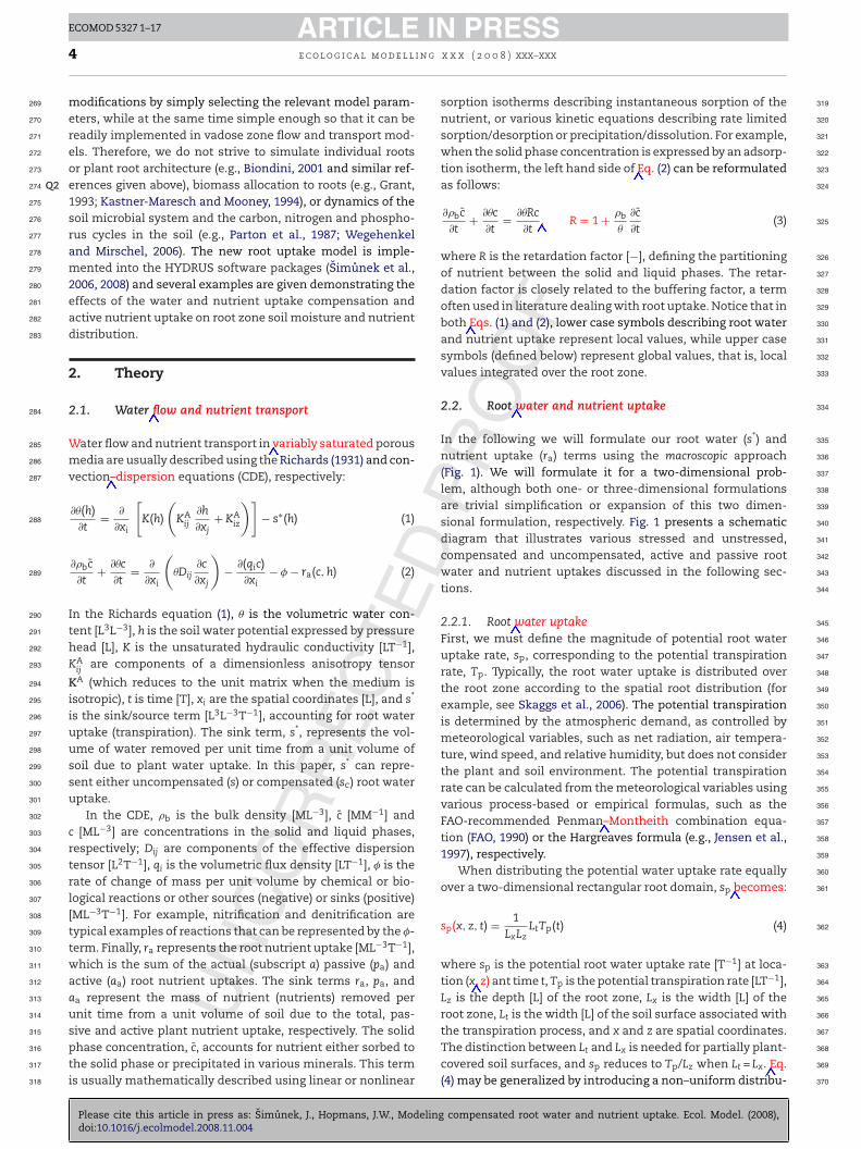
The presented examples will use the stress response func-tion of Feddes et al. (1978) (Fig. 3). Notice that water uptake isassumed to be zero close to saturation (i.e., wetter than somearbitrary “anaerobiosis point”, h1). For h < h4 (the wilting point
Fig. 3 – Schematic of the plant water stress responsefunction, ˛(h), as used by Feddes et al. (1978).
448
449
450
451
452
453
454
455
456
457
458
459
460
PR
OO
F
PRESSx x x ( 2 0 0 8 ) xxx–xxx
pressure head), water uptake is also zero. Water uptake is con-sidered optimal between pressure heads h2 and h3, whereasfor soil water pressure head values between h3 and h4 (or h1
and h2), water uptake decreases (or increases) linearly with h.For phreatic plants and trees that are able to extract water frombelow the groundwater, values of h1 and h2 can be adjusted,or set to zero in which case the Feddes’ function is similarto the Maas (1990) model. Parameters of the stress responsefunction for a majority of agricultural crops can be found invarious databases (e.g., Taylor and Ashcroft, 1972; Wesselinget al., 1991) and are directly implemented into the GUI ofHYDRUS. As is apparent from inspection of Eq. (7) the actualroot water uptake is equal to potential uptake (and potentialtranspiration) during periods of no water stress (˛(h) = 1).
The actual local uncompensated root water uptake, s, isobtained by substituting (5) into (8), or
s(h, h�, x, z, t) = ˛(h, h�, x, z, t)b(x, z, t)LtTp(t) (9)
so that the actual transpiration rate, Ta [LT−1], is obtained byintegrating (9) over the root domain ˝R, or
Ta(t) = 1Lt
∫˝R
s(h, h�, x, z, t) d˝
= Tp(t)
∫˝R
˛(h, h�, x, z, t)b(x, z, t) d˝ (10)
2.2.1.2. Compensated root water uptake. The ratio of actualand potential transpiration of uncompensated root wateruptake is defined as
Ta(t)Tp(t)
= 1Tp(t)Lt
∫˝R
s(h, h�, x, z, t) d˝
=∫
˝R
˛(h, h�, x, z, t)b(x, z, t) d˝ = ω(t) (11)
where ω is a dimensionless water stress index (Jarvis, 1989,1994). Following Jarvis (1989, 1994), we introduce a criticalvalue of the water stress index ωc, or the so-called root adapt-ability factor. It represents a threshold value, above which theroot water uptake reduced in stressed parts of the root zoneis fully compensated for by uptake from other, less-stressedparts (Fig. 4). Below this critical value, there is a certain reduc-tion of the potential transpiration, although smaller than inuncompensated root water uptake.
Defining compensated actual transpiration rate, Tac, as theratio of Ta/ω, the ratio of the actual to potential transpirationbecomes for the water stress range above the critical waterstress index (i.e., ω > ωc):
∫˛(h, h , x, z, t)b(x, z, t) d˝
ECOMOD 5327 1–17compensated root water and nutrient uptake. Ecol. Model. (2008),
Tac(t)Tp(t)
= Ta(t)Tp(t)ω(t)
= ˝R�
ω(t)= ω(t)
ω(t)= 1, 461
sc(h, h�, x, z, t) = ˛(h, h�, x, z, t)b(x, z, t)LtTp(t)ω(t)
(12) 462

D
ARTICLE INECOMOD 5327 1–17
e c o l o g i c a l m o d e l l i n g x
Fig. 4 – Ratio of the actual to potential transpiration as afunction of the stress index ω (arrows point towards thecorresponding axis; the left axis is for compensatedu
F463
(464
465
466
w467
a468
p469
t470
i471
ω472
p473
474
475
s476
e477
T478
479
U480
t481
i482
w483
e484
i485
p486
h487
c488
w489
490
491
492
493
494
495
496
497
498
499
500
501
502
503
504
505
506
507
508
509
510
511
512
513
514
515
516
517
518
519
520
521
522
523
524
525
526
527
528
529
530
531
532
533
534
535
536
537
538
539
540
541
542
543
544
NC
OR
RE
CTE
ptake, while the right axis is for uncompensated uptake).
or the water stress range below the critical water stress indexi.e., ω < ωc) we define Tac = Ta/ωc, so that
Tac(t)Tp(t)
= Ta(t)Tp(t)ωc(t)
=∫
˝R˛(h, h�, x, z, t)b(x, z, t) d˝
ωc= ω(t)
ωc< 1,
sc(h, h�, x, z, t) = ˛(h, h�, x, z, t)b(x, z, t)LtTp(t)ωc
(13)
here sc is the compensated root water uptake [T−1]. For ωc = 1nd 0, root water uptake is either uncompensated or fully com-ensated, respectively. We note that division by zero in (13) isheoretically not-defined. Uncompensated root water uptakes thus a special case of compensated root water uptake when
c = 1 (Fig. 1a). Combined, both uncompensated and (fully orartially) compensated models can be defined by
Tac(t)Tp(t)
=∫
˝R˛(h, h�, x, z, t)b(x, z, t) d˝
max[ω(t), ωc]= ω(t)
max[ω(t), ωc]≤ 1,
sc(h, h�, x, z, t) = ˛(h, h�, x, z, t)b(x, z, t)LtTp(t)
max[ω(t), ωc](14)
o that the total actual compensated plant transpiration isqual to
ac(t) = 1Lt
∫˝R
sc(h, h�, x, z, t) d˝
= Tp(t)max[ω(t), ωc]
∫˝R
˛(h, h�, x, z, t)b(x, z, t) d˝ (15)
sing this approach, water uptake compensation is propor-ional to the water stress response function. Water uptakencrease (compensation) is maximum in parts of the root zone
here the root water uptake is optimal (i.e., not reduced),qual to zero in parts of the root zone where the pressure heads below the wilting point or above the anaerobiosis point; and
UPlease cite this article in press as: Simunek, J., Hopmans, J.W., Modelingdoi:10.1016/j.ecolmodel.2008.11.004
roportional to the water stress response for other pressureead values. In this way, the proposed compensation model islosely related to models based on minimizing energy of rootater uptake (e.g., Adiku et al., 2000; Van Wijl and Bouten,
PR
OO
F
PRESSx x ( 2 0 0 8 ) xxx–xxx 7
2001). We note that this compensation mechanism spatiallyredistributes root water uptake from stressed to less-stressedregions of the root zone, where water is held with smaller cap-illary forces and thus more easily available for the plant. Thisis very different than simply modifying the stress responsefunction by expanding the pressure head intervals for bothunlimited and limited uptake across the whole rooting zone.
However, as pointed out by Skaggs et al. (2006), the pre-sented compensation is conceptually unsound, if the wholeroot domain is equally stressed. For example, the model willpredict a full compensation of root water uptake when theroot zone has the uniform pressure head for which the wateruptake is reduced by less than the critical water stress index.The predicted root water uptake, which is uniform under suchconditions throughout the root zone, will then deviate, due tocompensation, from the value predicted by the stress responsefunction. To overcome this conceptual problem one can, forexample, consider compensation of root water uptake to occur(a) only from parts of the root zone which are not stressed atall or (b) from zones which are stressed less than ω. After suchmodification, the updated compensated root water uptakemodel will follow the thick line from Fig. 4 only when thepressure head in a part of the root zone is below the wilt-ing point and the rest is either non-stressed or stressed lessthan ω, respectively. For all other conditions, the model will bebetween theoretical lines for non-compensated and compen-sated root water uptake.
The compensated root water uptake model requires asinput the potential evapotranspiration rate Tp, the spatialroot distribution function b(x, z, t), the water stress responsefunction ˛, and the critical water stress index ωc. Therefore,the additional new input variable, as compared to traditionaluncompensated root water uptake is the critical water stressindex, ωc. It can be expected that cultural (i.e., agricultural)plants have a relatively high ωc and thus their ability to com-pensate natural stresses is limited, as compared to naturalplants, especially desert species, that have a low ωc and cor-respondingly high ability to compensate for natural stresses(i.e., to only take up water and nutrients from those parts ofthe root system where they are most available).
2.2.2. Root nutrient uptakeThe presented model allows for both passive and active rootnutrient uptake. Whereas passive uptake describes the massflow and root uptake of nutrients dissolved in water taken upby plant roots, we define active uptake as all other possiblenutrient uptake mechanisms, including energy-driven pro-cesses against electrochemical gradients. The term “passiveuptake” is used here, and throughout the manuscript, to repre-sent flow of nutrients into roots associated with flow of watersupplying the plant transpiration demand. Since transpirationflow is an active process, the mass nutrient flow is also a pro-cess that is actively regulated by plants. The terms “passive”and “active” are used here mainly to distinguish between thesetwo mechanisms of root nutrient uptake.
Similarly, as for root water uptake, we define a poten-
ECOMOD 5327 1–17compensated root water and nutrient uptake. Ecol. Model. (2008),
tial nutrient demand, Rp [ML−2T−1], that depends on the 545
plant physiological growth stage, supplied by both passive and 546
active nutrient uptake. Daily nutrient consumption rates are 547
known for various field crops as a function of their growth 548
ED
INECOMOD 5327 1–17
i n g
549
550
551
552
553
554
555
556
557
558
559
560
561
562
563
564
565
566
567
568
569
570
571
572
573
574
575
576
577
578
579
580
581
582
583
584
585
586
587
588
589
590
591
592
593
594
595
596
597
598
599
600
601
602
603
604
605
606
607
608
609
610
611
612
613
614
615
616
617
618
619
620
621
622
623
624
625
626
627
628
629
630
631
632
633
634
635
636
637
638
639
640
641
642
643
NC
OR
RE
CT
ARTICLE8 e c o l o g i c a l m o d e l l
stage (after emergence or planting), for example as reportedby Bar-Yosef (1999) for N, P, and K nutrients.
We further assume that passive uptake is the primarymechanism of supplying plants with nutrients, and that activeuptake is initiated only if passive uptake is inadequate. Fortheir physiological development, plants need to take up waterfrom the root zone, and as nutrients are dissolved in soilwater they can enter the plant by the dissolved water phasepathway. The active uptake will then provide additional nutri-ents that are required beyond what is supplied by passiveuptake. In general, the presented model allows for both pas-sive and active nutrient uptake mechanism to occur separatelyor simultaneously, as described below. The relative signifi-cance of active and passive nutrient uptakes in supplyingvarious agricultural crops with nutrients can be found in theliterature. For example, values for N, P, and K in maize are givenby Jungk (1991).
2.2.2.1. Uncompensated nutrient uptake model. To clearly dif-ferentiate between point and root domain nutrient uptakerate values, we define lower case variables to represent pointroot nutrient uptake rates [ML−3T−1], while upper case vari-ables represent nutrient uptake rates [ML−2T−1] over the entiretwo-dimensional root zone domain, ˝R. Both point and rootdomain nutrient uptakes are assumed to be the sum of theirpassive and active components, or
ra(x, z, t) = pa(x, z, t) + aa(x, z, t) (16)
Ra(t) = Pa(t) + Aa(t) (17)
where ra, pa, and aa define total actual (subscript a) passiveand active root nutrient uptake rates [ML−3T−1], respectively,at any point, and Ra, Pa, and Aa denote actual total, passiveand active root nutrient uptake rates [ML−2T−1], respectively,for the root zone domain.
Passive nutrient uptake is simulated by multiplying rootwater uptake (compensated or uncompensated) with the dis-solved nutrient concentration, for concentration values belowa priori defined maximum concentration (cmax), or
pa(x, z, t) = s∗(x, z, t) min[c(x, z, t), cmax] (18)
where c is the dissolved nutrient concentration [ML−3] andcmax is the maximum allowed solution concentration [ML−3]that can be taken up by plant roots during passive root uptake.All nutrient dissolved in water is taken up by plant roots whencmax is large (larger than the dissolved concentration c), whileno nutrient is taken up when cmax is equal to zero, with onlyactive uptake remaining in that case (Fig. 1b). The maximumsolution concentration for passive root uptake, cmax, thus con-trols the relative proportion of passive root water uptake tototal uptake. Using this flexible formulation, uptake mecha-nisms can vary between specific nutrients. For example, Nauptake can be excluded by setting cmax equal to zero, passiveCa uptake can be limited by defining a finite c value, or all
UPlease cite this article in press as: Simunek, J., Hopmans, J.W., Modelingdoi:10.1016/j.ecolmodel.2008.11.004
max
soil solution available P or N is allowed to be taken up pas-sively, by setting cmax to a very large value. Note that the cmax
parameter is introduced as a control model parameter thatdoes not necessarily have a physiological meaning.
PR
OO
F
PRESSx x x ( 2 0 0 8 ) xxx–xxx
Passive actual root nutrient uptake for the whole rootdomain, Pa [ML−2T−1], is calculated by integrating the localpassive root nutrient uptake rate, pa, over the entire root zone,or after applying Eq. (14):
Pa(t) = 1Lt
∫˝R
pa(x, z, t) d˝
= 1Lt
∫˝R
s∗(x, z, t) min[c(x, z, t), cmax] d˝
= Tp(t)max[ω(t), ωc]
∫˝R
˛(h, h�, x, z, t)b(x, z, t) min[c(x, z, t), cmax] d˝ (19)
Defining Rp as the potential (subscript p) nutrient demand[ML−2T−1], the potential active nutrient uptake rate, Ap
[ML−2T−1], is computed from:
Ap(t) = max[Rp(t) − Pa(t), 0] (20)
Thus, using this formulation, we assume that active nutrientuptake will be invoked only if the passive root nutrient uptaketerm does not fully satisfy the potential nutrient demandof the plant. However, as was discussed earlier, the passiveuptake can be reduced or completely turned off (cmax = 0), thusallowing the potential active nutrient uptake (Ap) to be equalto the potential nutrient demand (Rp). Once Ap is known,the point values of potential active nutrient uptake rates, ap
[ML−3T−1], are obtained by distributing the potential root zoneactive nutrient uptake rate, Ap [ML−2T−1], over the root zonedomain, using a predefined spatial root distribution, b(x, z, t),as was done for root water uptake in Eq. (5), or
ap(x, z, t) = b(x, z, t)LtAp(t) (21)
Using Michaelis–Menten kinetics (e.g., Jungk, 1991) providesfor actual distributed values of active nutrient uptake rates,aa [ML−3T−1], allowing for nutrient concentration dependency,or
aa(x, z, t) = c(x, z, t) − cmin
Km + c(x, z, t) − cminap(x, z, t)
= c(x, z, t) − cmin
Km + c(x, z, t) − cminb(x, z, t)LtAp(t) (22)
where Km is the Michaelis–Menten constant [ML−3] and cmin
is the minimum nutrient concentration required for activeuptake to take effect [ML−3] (Jungk, 1991), thus assuming thatactive nutrient uptake will occur only if the dissolved nutrientconcentration in the soil solution is sufficiently high. Otherapproaches have been suggested to deal with the concen-tration threshold (Silberbush, 2002). The Michaelis–Mentenconstants for selected nutrients (e.g., N, P, and K) and plantspecies (e.g., corn, soybean, wheat, tomato, pepper, lettuce,and barley) can be found in the literature (e.g., Bar-Yosef,
ECOMOD 5327 1–17compensated root water and nutrient uptake. Ecol. Model. (2008),
1999). Though not in agreement with the presented concept of 644
distinguishing between passive and active uptake, the formu- 645
lation could be easily modified so that the Michaelis–Menten 646
kinetics is applied to the sum of the active and passive nutri- 647
D
ARTICLE INECOMOD 5327 1–17
e c o l o g i c a l m o d e l l i n g x
Fig. 5 – Ratio of actual to potential active nutrient uptake asa function of the stress index � (arrows point towards thecu
e648
2649
650
r651
a652
r653
w654
A655
656
657
2658
e659
n660
s661
s662
E663
r664
�665
A666
v667
i668
�669
A670
�671
c672
s673
e674
n675
o676
a677
678
679
680
681
682
683
684
685
686
687
688
689
690
691
692
693
694
695
696
697
698
699
700
701
702
703
704
705
706
707
708
709
710
711
712
713
714
715
716
717
718
719
720
721
NC
OR
RE
CTE
orresponding axis; the left axis is for compensatedptake, while the right axis is for uncompensated uptake).
nt uptake as it is usually used in the literature (Silberbush,002).
Finally, total active uncompensated root nutrient uptakeate, Aa [ML−2T−1], is calculated by integrating the actualctive root nutrient uptake rate, aa, at each point, over theoot domain ˝R, in analogy with the non-compensated rootater uptake term in Eq. (10), or
a(t) = 1Lt
∫˝R
aa(x, z, t) d˝
= Ap(t)
∫˝R
c(x, z, t) − cmin
Km + c(x, z, t) − cminb(x, z, t) d˝ (23)
.2.2.2. Compensated nutrient uptake model. The above nutri-nt uptake model includes compensation of the passiveutrient uptake, by way of the root water uptake compen-ation term, sc, and root adaptability factor, ωc, in Eq. (19). Aimilar compensation concept as used for root water uptake inqs. (11) and (12), was implemented for active nutrient uptakeate, by invoking a so-called nutrient stress index �:
(t) = Aa(t)Ap(t)
(24)
fter substitution of the active total root nutrient uptake ratealue from Eq. (23) above, this newly defined nutrient stressndex (�) is equal to
(t) =∫
˝R
c(x, z, t) − cmin
Km + c(x, z, t) − cminb(x, z, t) d˝ (25)
fter defining the critical value of the nutrient stress index
c (Fig. 5), above which value active nutrient uptake is fullyompensated for by active uptake in other more-available (lesstressed) soil regions, the local compensated active root nutri-nt uptake rate, aac [ML−3T−1], is obtained by including theutrient-stress index function in the denominator of Eq. (22),
UPlease cite this article in press as: Simunek, J., Hopmans, J.W., Modelingdoi:10.1016/j.ecolmodel.2008.11.004
r
ac(x, z, t) = c(x, z, t) − cmin
Km + c(x, z, t) − cminb(x, z, t)Lt
Ap(t)max[�(t), �c]
(26)
PR
OO
F
PRESSx x ( 2 0 0 8 ) xxx–xxx 9
from which the total compensated active root nutrient uptakerate, Aac [ML−2T−1] in the two-dimensional root domain, ˝R,is calculated, in analogy with the compensated root wateruptake term in Eq. (15), as follows:
Aac(t) = 1Lt
∫˝R
aac(x, z, t) d˝
= Ap(t)max[�(t), �c]
∫˝R
c(x, z, t) − cmin
Km + c(x, z, t) − cminb(x, z, t) d˝
(27)
Eq. (20) implies that reduction in root water uptake willdecrease passive nutrient uptake, thereby increasing activenutrient uptake proportionally. In other words, total nutrientuptake is not affected by soil water stress, as computed bythe proportion of actual to potential root water uptake. Thisis not realistic since one would expect that plant nutrientrequirements will be reduced for water-stressed plants. Forthat reason, the uptake model includes additional flexibility,by reducing the potential nutrient demand Rp [ML−2T−1], inproportion to the reduction of root water uptake, as definedby the actual to potential transpiration ratio, or
Ap(t) = max
[Rp(t)
Tac(t)Tp(t)
− Pa(t), 0
](28)
In summary, the presented root nutrient uptake model withcompensation requires as input the potential nutrient uptakerate (demand), Rp, the spatial root distribution function b(x, z,t) as needed for the water uptake term, the Michaelis–Mentonconstant Km, the maximum nutrient concentration that can betaken up passively by plant roots cmax, the minimum concen-tration cmin needed to initiate active nutrient uptake, and thecritical nutrient stress index �c. The passive nutrient uptaketerm can be turned off by selecting cmax equal to zero. More-over, active nutrient uptake can be eliminated by specifying azero value for Rp in Eq. (20), or by selecting a very large cmin
value in Eq. (22). It is likely that values of these parameters arenutrient- and plant-specific. Similarly as for root water uptake,it can be expected that �c for agricultural crops is relativelyhigh when compared to natural plants that are likely to havemore ability to compensate for soil environmental stresses.Other parameters, such as cmax will likely need to be cali-brated to specific conditions before the model can be used forpredictive purposes.
3. Numerical implementation
Both the Richards equation (1) and the convection–dispersionequation (2) are solved in HYDRUS code (Simunek et al., 2006,2008) using the finite element method in the spatial domainand the finite differences method in the temporal domain.Implementation of the compensated root water and nutrientuptake routines did require changing the numerical approach
ECOMOD 5327 1–17compensated root water and nutrient uptake. Ecol. Model. (2008),
to solve these governing equations. However, a two- or three- 722
step approach was needed to calculate the compensated root 723
water and nutrient uptake with passive and active compo- 724
nents, respectively, for each time step. 725
ED
PR
OO
F
IN PRESSECOMOD 5327 1–17
i n g x x x ( 2 0 0 8 ) xxx–xxx
726
727
728
729
730
731
732
733
734
735
736
737
738
739
740
741
742
743
744
745
746
747
748
749
750
751
752
753
754
755
756
757
758
759
760
761
762
763
764
765
766
767
768
769
770
771
772
773
774
775
776
777
778
779
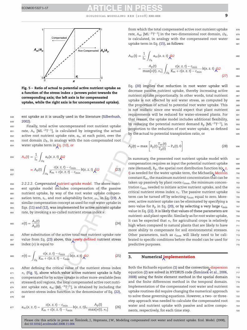
Fig. 6 – Example 1. Root water uptake (top) and soil waterpressure head (bottom) profiles for uncompensated (solidthick lines) and compensated root water uptake with values
780
781
782
783
784
785
786
787
788
789
790
791
792
793
NC
OR
RE
CT
ARTICLE10 e c o l o g i c a l m o d e l l
In the root water uptake module, the uncompensated rootwater uptake (9) and the dimensionless water stress index ω
(11) are evaluated in the first iteration step, which is the onlystep needed when compensated root water uptake is not con-sidered. The compensated root water uptake (13) is evaluatedin the second step, prior to solving the Richards equation (1).
A multiple-step approach was required to evaluate theroot nutrient uptake term. Only one step is needed, whenonly passive or no root nutrient uptake is considered. If non-compensated active root nutrient uptake is considered, atwo-step approach is required. In this case, passive nutri-ent uptake (18) and potential active nutrient uptake rate Ap
(20) are evaluated in the first step, whereas uncompensatedactive root nutrient uptake (22) is evaluated during the sec-ond step. The additional third step is needed if compensatedactive root water uptake is considered. In that case, the nutri-ent stress index � (24) is first evaluated during the second step,so that the compensated active root nutrient uptake (26) canbe evaluated in the third step, prior to solving the convec-tion–dispersion equation (2).
4. Examples
The functioning of compensated root water uptake is demon-strated for three examples. While the first example considersa simple one-dimensional soil profile, the second exampleapplies to an axi-symmetrical three-dimensional water flowand nutrient transport domain. In the third example wedemonstrate the consequences of the various presented nutri-ent uptake models, including both passive and active nutrientuptake, with and without compensation. All examples applyto the same loamy soil, for which the soil hydraulic proper-ties were taken from Carsel and Parrish (1988). Also, the samesoil water stress response function of Feddes et al. (1978) inFig. 3 was used for all examples, with h1 = −10 cm, h2 = −25 cm,h3,high = −200 cm, h3,low = −800 cm, and h4 = −8000 cm. The trueh3 parameter is interpolated from h3,high and h3,low and Tp (seeFig. 3), as done in the SWATRE code (e.g., Wesseling et al., 1991).
4.1. Root water uptake in a one-dimensional soilprofile with groundwater table
The first example applies to a one-dimensional 120-cm soilprofile with a 90-cm root depth and the root distribution lin-early decreasing with depth. The bottom of the soil is boundedby a ground water table that is in hydrostatic equilibrium withthe soil profile at the start of the simulation (initial condi-tion). The hypothetical plant is assumed to transpire with apotential transpiration rate, Tp, of 0.4 cm/day, while the waterstress index ωc is varied with values of 1.0 (corresponding touncompensated root water uptake), 0.75 and 0.5, with the lat-ter two values corresponding with increasing compensatedroot water uptake as the index decreases. Since this set ofmodel simulations does not include precipitation or irrigation,water required for transpiration will deplete the soil water pro-
UPlease cite this article in press as: Simunek, J., Hopmans, J.W., Modelingdoi:10.1016/j.ecolmodel.2008.11.004
file so that the resulting soil water potential (h) gradient willpartially supply the root zone with water, driven by capillaryrise from the shallow groundwater. Simulations were carriedout for a total period of 50 days.
794
of ωc = 0.75 (solid thin lines) and 0.5 (dashed thick lines).
Fig. 6 presents the depth distribution of root water uptake,s* (day−1) and soil water pressure head, h (cm), along thesoil profile for the uncompensated (ωc = 1.0) and compensated(ωc = 0.75 or 0.5) root water uptake scenarios, whereas Fig. 7 isa plot of both actual (cm/d) and cumulative values (cm) of thepotential (Tp) and actual (Ta) transpirations, and water flux atthe groundwater table for the three corresponding scenariosduring the 50-day simulation period. As Figs. 6 and 7 show, thenon-compensated root water uptake starts to decrease aroundthe 10th day (Fig. 6) as a result of water stress, with the top20 cm of the soil profile being fully depleted of water (Fig. 7)after about 20 days of plant transpiration. For the 30–90 cmsoil depth, capillary rise provides for sufficient water supplytowards the rooting zone, thus allowing the lower root domainto remain unstressed with root water uptake at the normal
ECOMOD 5327 1–17compensated root water and nutrient uptake. Ecol. Model. (2008),
unstressed uptake rate. Root water uptake rates after about 795
10 days are always either equal or lower than the root water 796
uptake at the beginning of the simulations. 797

CTE
D
ARTICLE INECOMOD 5327 1–17
e c o l o g i c a l m o d e l l i n g x
Fig. 7 – Example 1. The potential transpiration (black), theactual transpiration (red), and the bottom flux (blue) (top)and their cumulative values (bottom) for uncompensatedQ4
(solid thick lines) and compensated (ωc = 0.75, solid thinlines; ωc = 0.5, dashed thick lines) root water uptakescenarios. (For interpretation of the references to color inthis figure legend, the reader is referred to the web versiono
798
u799
t800
d801
u802
p803
t804
r805
r806
p807
w808
u809
s810
s811
812
r813
u814
u815
2816
817
818
819
820
821
822
823
824
825
826
827
828
829
830
831
832
Q3 833
834
835
836
837
838
839
840
841
842
843
844
845
846
847
848
849
850
851
852
853
854
855
856
857
858
859
860
861
862
863
864
865
866
867
868
869
870
NC
OR
REf the article.)
For the scenarios that considered compensated root waterptake, a reduction in the uptake from the upper part ofhe profile is initially fully compensated by uptake from theeeper part of the soil profile. Root water uptake rates grad-ally increase in deeper parts of the soil profile as the upperart of the root zone becomes more stressed. The compensa-ion from larger soil depths is larger for lower values of ωc. As aesult, the root water uptake distribution in Fig. 6 moves to theight as time increases; and increasingly so for the more com-ensated uptake (ωc = 0.5) scenario. Since compensated rootater uptake is greater than the uncompensated root waterptake at the bottom of the root zone, a larger fraction of theoil profile is water-depleted, thus capillary rise will need toupply a smaller fraction of the root zone.
As a result of water stress, Fig. 7 shows that actual transpi-
UPlease cite this article in press as: Simunek, J., Hopmans, J.W., Modelingdoi:10.1016/j.ecolmodel.2008.11.004
ation (Ta) starts to deviate from Tp already after 10 days for thencompensated scenario, whereas compensated root waterptake continues to be at a potential rate until days 20 and7 for scenarios with values of ωc = 0.75 and 0.5, respectively.
PR
OO
F
PRESSx x ( 2 0 0 8 ) xxx–xxx 11
During this time period, a reduced uptake from the upper partof the soil profile is fully compensated for by an increaseduptake from deeper soil profile. Root water uptake remainssignificantly higher for the compensated scenarios even whenit is reduced from its potential values at later times. Cumula-tive actual transpiration during the 50 day period increasesfrom about 13.7 to 15.0 and 16.7 cm for the uncompensatedand compensated (ωc = 0.75 and 0.5) root water uptake scenar-ios, respectively. Daily values of Ta at the end of the simulationperiod increase from 0.17, to 0.19, and 0.235 cm/day for thesethree scenarios, resulting in an increase in cumulative planttranspiration by almost 40%. Neglecting root water uptakecompensation by plant roots in water-stressed soil conditionswould thus result into significant errors in plant transpirationand the soil water balance. The presented interactions of rootwater uptake and soil moisture and their spatial variationsconfirm experimental studies by Green and Clothier (1995) andAndreu et al. (1997), with the shifting of preferential root wateruptake to the wetter parts of the soil system after irrigation orthe development of water uptake fronts moving downwards asthe soil dries (Doussan et al. (2006). Irrespective of the selectedscenario, near steady-state conditions were attained at theend of the 50-day simulation period, with actual transpira-tion fully supplied by the capillary rise from the ground watertable. Similar results were obtained when considering morerealistic diurnal plant transpiration variations similar to nat-ural conditions (0.24 Tp during night time (6 pm to 6 am) and2.75Tp sin(2�t/tPeriod − �/2) during the day).
4.2. Root water uptake for an axi-symmetricalthree-dimensional profile with irrigation
In the second example we considered an axi-symmetrical flowdomain for which both depth and radius values are equal to100 cm. The initial pressure head (t = 0) was −400 cm through-out the soil profile and the potential transpiration rate was0.04 cm/h. While water needed for transpiration was suppliedby capillary rise from the shallow water table in the first exam-ple, water was supplied by irrigation for the example twoscenarios. Irrigation water application was confined to a 50-cm radius around the center of the simulation domain, at aconstant rate of 0.16 cm/h. Since this irrigated area is 4 timessmaller than the flow domain, the irrigation flux of four timesthe value of Tp was exactly equal to the transpiration demand.Root density was assumed to decrease linearly from its maxi-mum value to zero at the 50 cm soil depth, but to be constantin the radial direction. The water stress index ωc was variedfrom 1.0 to 0.4, using increments of 0.2.
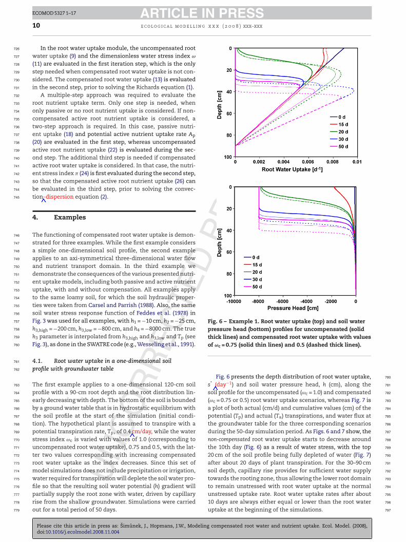
Fig. 8 presents both actual and cumulative values of thepotential and actual transpiration rates. While only a limitedreduction in transpiration (0.038 cm/h) was attained for thecompensated root water uptake scenario with ωc = 0.4, rootwater uptake for the uncompensated scenario was reducedby exactly one half (0.020 cm/h). For the other scenarios withωc values of 0.6 and 0.8, Ta was reduced to 0.29 and 0.24 cm/h,respectively. With the uncompensated root water uptake sce-
ECOMOD 5327 1–17compensated root water and nutrient uptake. Ecol. Model. (2008),
nario being reduced immediately as the initial pressure head 871
was already on the declining part of the water stress response 872
function (Fig. 3), plant water uptake for the compensated root 873
water uptake scenarios started to decrease from potential val- 874
CTE
D P
RO
OF
ARTICLE IN PRESSECOMOD 5327 1–17
12 e c o l o g i c a l m o d e l l i n g x x x ( 2 0 0 8 ) xxx–xxx
Fig. 8 – Example 2. The potential (black line) and actualtranspirations for scenarios with the water stress index ωc
equal to 1.0 (pink), 0.8 (blue), 0.6 (green), and 0.4 (red).Actual values are shown at the top, while cumulativevalues at the bottom. (For interpretation of the references tocolor in this figure legend, the reader is referred to the web
875
876
877
878
879
880
881
882
883
884
885
886
887
888
889
890
891
892
893
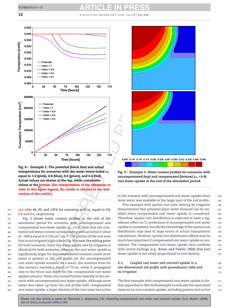
Fig. 9 – Example 2. Water content profiles for scenarios with
894
895
896
897
898
899
900
901
902
903
904
905
906
907
908
909
910
UNCO
RR
Eversion of the article.)
ues after 44, 60, and 120 h for scenarios with ωc equal to 0.8,0.6 and 0.4, respectively.
Fig. 9 shows water content profiles at the end of thesimulation period for scenarios with uncompensated andcompensated root water uptake (ωc = 0.4). Note that the volu-metric soil water content corresponding with an initial h-valueof −400 is equal to 0.156 cm3 cm−3. The portion of the root zonethat is not irrigated (right side in Fig. 9) is near the wilting pointfor both scenarios. Since the water supply rate by irrigation isidentical for both scenarios, whereas the root water uptake issignificantly larger for the compensated scenario, much morewater is present in the soil profile for the uncompensatedroot water uptake scenario. As a result, the moisture front forthis scenario reached a depth of 75 cm, while it propagatedonly to the 60 cm soil depth for the compensated root water
Please cite this article in press as: Simunek, J., Hopmans, J.W., Modelingdoi:10.1016/j.ecolmodel.2008.11.004
uptake scenario. Water also moved further laterally in the sce-nario with uncompensated root water uptake. Although morewater was taken up from the soil profile with compensatedroot water uptake, a larger fraction of the root zone was active
uncompensated (top) and compensated (bottom) (ωc = 0.4)root water uptake at the end of the simulation period.
in the scenario with uncompensated root water uptake sincemore water was available in the larger part of the soil profile.
This example with partial root zone wetting by irrigationdemonstrated that potential plant water demand can be sat-isfied when compensated root water uptake is considered.Therefore, spatial root distribution is expected to have a sig-nificant effect on Ta predictions if uncompensated root wateruptake is considered. Insufficient knowledge of the spatial rootdistribution may lead to large errors in actual transpirationcalculations. However, spatial root distribution effects may bemuch less important if compensated root water uptake is con-sidered. The compensated root water uptake thus confirmswith recent findings (e.g., Roose and Fowler, 2004) that rootwater uptake is not solely proportional to root density.
4.3. Coupled root water and nutrient uptake in aone-dimensional soil profile with groundwater table andno irrigation
ECOMOD 5327 1–17compensated root water and nutrient uptake. Ecol. Model. (2008),
The first example with compensated root water uptake is fur- 911
ther expanded in this third example to evaluate the associated 912
impacts on root nutrient uptake, including passive and active 913

D P
RO
OF
IN PRESSECOMOD 5327 1–17
g x x x ( 2 0 0 8 ) xxx–xxx 13
c914
a915
s916
l917
n918
s919
u920
p921
n922
a923
924
T925
t926
p927
a928
(929
e930
s931
w932
s933
t934
t935
n936
T937
t938
939
v940
l941
a942
w943
c944
i945
i946
D947
t948
(949
b950
w951
c952
u953
t954
i955
i956
r957
u958
c959
t960
t961
r962
963
c964
b965
c966
t967
v968
r969
d970
r971
m972
r973
Fig. 10 – Example 3. Depth distribution of nutrientconcentration for nutrient uptake scenarios considering (a)no nutrient uptake (top) and (b) passive nutrient uptake
974
975
976
977
978
979
980
981
982
983
984
985
986
987
988
NC
OR
RE
CTE
ARTICLEe c o l o g i c a l m o d e l l i n
onsiderations. To simplify this analysis, nutrient transportnd uptake was coupled with the example 1 scenario that con-idered uncompensated root water uptake only (thick solidines in Figs. 6 and 7 with ωc = 1.0). We compared six rootutrient uptake scenarios: (a) no nutrient uptake, (b) only pas-ive nutrient uptake (i.e., no active uptake), (c) passive andncompensated active nutrient uptake, (d) passive and com-ensated active nutrient uptake, (e) uncompensated activeutrient uptake (i.e., no passive uptake), and (f) compensatedctive nutrient uptake (i.e., no passive uptake).
Calculations were carried out in relative concentrations.he initial nutrient concentrations in the soil profile and in
he ground water were both assumed to be equal to one. Theotential nutrient demand, Rp, for scenarios that involvedctive root nutrient uptake was assumed to be equal to 1−/cm2 day) as well, whereas its value was set to zero for thexample scenarios without an active root nutrient uptake. Forcenarios that excluded passive root nutrient uptake, the cmax
as set equal to 0, while its value was set to 10 (larger than anyimulated dissolved soil solution concentration) for scenarioshat include passive root nutrient uptake. The critical value ofhe nutrient stress index, �c, was assumed equal to 0.5 for sce-arios that allowed compensated active root nutrient uptake.he Michaelis–Menten constant, Km, was set to 0.1, whereas
he minimum concentration, cmin, was assumed zero.While Figs. 10 and 11 shows concentration profiles for the
arious root nutrient uptake scenarios, the actual and cumu-ative nutrient uptake rates as a function of simulation timere presented in Fig. 12. It is specifically noted that scenariosithout any nutrient uptake lead to an increase in nutrient
oncentrations in the root zone (Fig. 10, top), and that scenar-os that allow active nutrient uptake will lead to a decreasen soil nutrient concentration (Figs. 11) as time progresses.issolved soil solution concentrations gradually increase in
he root zone for the scenario that neglects nutrient uptakeFig. 10, top), as caused by decreased volumetric water contenty root water uptake. Since water content gradually decreaseshile the amount of dissolved ions in the root zone remains
onstant, the resulting soil solution concentrations will grad-ally increase. Concentrations increase initially fastest closeo the soil surface, because the root water uptake is highestn this region. Concentrations in this zone tend to not furtherncrease, after the soil water content is depleted, thus limitingoot water uptake by soil water stress. However, as root waterptake continues from deeper soil regions, concentrations willontinue to increase there. The increase in nutrient concentra-ions might eventually affect the soil’s osmotic potential andhus cause salinity stress, in addition, thereby further reducingoot water uptake.
As expected, there will be no change in soil nutrient con-entrations when nutrient uptake is only passive (Fig. 10,ottom), since there are no mechanisms in place that wouldause concentration gradients in the soil profile to develop,hus eliminating diffusion/dispersion to occur. Since the cmax
alue was set to be above soil solution concentrations, wateremoved from the root zone by root uptake takes along all
UPlease cite this article in press as: Simunek, J., Hopmans, J.W., Modelingdoi:10.1016/j.ecolmodel.2008.11.004
issolved ions, while water left behind in the root zone willemain at constant concentrations. Yet, the total soil nutrient
ass will decrease, because of the passive nutrient uptake andeduction in water contents.
only (bottom).
Soil solution nutrient concentrations will graduallydecrease throughout the soil profile for those scenarios withactive nutrient uptake (Fig. 11), leading to early nutrientdepletion in the near soil surface regions of the profile. Thisdepletion is faster for scenarios with compensated root nutri-ent uptake. We note that there is only a small difference inthe depth distribution of nutrient concentration for scenariosthat consider (both uncompensated and compensated) activenutrient uptake, irrespective of whether passive nutrientuptake is allowed.
It is important to realize that the absence of nutrient uptakewill result in an increase in soil solution concentration as aconsequence of root water uptake. No concentration changeswere computed for those scenarios where nutrient uptake issolely by passive nutrient uptake, whereas all scenarios that
ECOMOD 5327 1–17compensated root water and nutrient uptake. Ecol. Model. (2008),
involved active nutrient uptake led to a significant decrease in 989
soil solution nutrient concentration. 990
Fig. 12 presents the actual and cumulative total plant 991
nutrient uptakes for scenarios where nutrient uptake was 992

CTE
D P
RO
OF
ARTICLE IN PRESSECOMOD 5327 1–17
14 e c o l o g i c a l m o d e l l i n g x x x ( 2 0 0 8 ) xxx–xxx
Fig. 11 – Example 3. Depth distribution of nutrientconcentration for nutrient uptake scenarios consideringeither uncompensated (top) or compensated (bottom) activenutrient uptake with (solid line) or without (dashed line)
993
994
995
996
997
998
999
1000
1001
1002
1003
1004
1005
1006
1007
1008
1009
Fig. 12 – Example 3. The actual (top) and cumulative(bottom) nutrient uptakes for scenarios considering (a) onlypassive nutrient uptake (black line), (b) passive anduncompensated active nutrient uptake (red lines), (c)passive and compensated active nutrient uptake (bluelines), (d) uncompensated active nutrient uptake (greenline), and (e) compensated active nutrient uptake (brownline). Thin and dashed lines represent active and passivenutrient uptake components, respectively. (Forinterpretation of the references to color in this figurelegend, the reader is referred to the web version of the
1010
1011
1012
1013
1014
1015
1016
1017
1018
1019
1020
1021
UNCO
RR
Epassive nutrient uptake.
considered. For scenarios where active and passive nutrientuptakes were simultaneously considered, Fig. 12 addition-ally also shows both active and passive components of thenutrient uptake. When only the passive nutrient uptake isconsidered, total nutrient uptake is directly proportional toroot water uptake as the dissolved soil solution concentrationsremain constant. When both active and passive root nutri-ent uptakes are considered, the total uptake is significantlylarger than when only the passive component is allowed.The total root nutrient uptake is initially equal to the poten-tial nutrient demand, if nutrient uptake from regions withsufficient nutrients present can compensate for uptake fromnutrient-depleted soil depths. The passive nutrient uptake is
Please cite this article in press as: Simunek, J., Hopmans, J.W., Modelingdoi:10.1016/j.ecolmodel.2008.11.004
significantly smaller when also active uptake is considered,since active uptake leads to lowering of dissolved concentra-tions that are involved in the passive uptake. The total nutrientuptake is relatively similar for scenarios that consider the
article.)
active uptake, irrespectively if the passive uptake is active ornot. When the passive nutrient uptake is neglected, the activeuptake correspondingly increases, resulting to similar results.As groundwater is the only source of water and nutrients, theroot nutrient uptake eventually decreases with time, similarlyas the root water uptake. Additional irrigation and fertigationwould be needed to sustain water and nutrient uptake at itspotential values.
The presented modeling results conform to many exper-imental nutrient uptake that show compensation andenhanced nitrate uptake responses by differential nitrate sup-ply (Robinson, 1994, 1996). Moreover, enhanced local nutrient
ECOMOD 5327 1–17compensated root water and nutrient uptake. Ecol. Model. (2008),
uptake to meet total plant nutrient demand supports the 1022
notion that local root uptake rate is not only dependent on the 1023
local environment, but also on the environmental conditions 1024
of the whole root system (Dunbabin et al., 2002).

D
INECOMOD 5327 1–17
g x
5
A1025
s1026
s1027
t1028
f1029
o1030
s1031
1032
o1033
m1034
o1035
o1036
o1037
c1038
s1039
t1040
t1041
u1042
t1043
w1044
1045
a1046
m1047
n1048
s1049
a1050
n1051
m1052
a1053
y1054
1055
d1056
i1057
b1058
e1059
d1060
p1061
i1062
m1063
i1064
t1065
w1066
1067
t1068
e1069
n1070
t1071
c1072
t1073
t1074
1075
c1076
e1077
n1078
n1079
e1080
n
1081
1082
1083
1084
r1085
1086
1087
1088
1089
1090
1091
1092
1093
1094
1095
1096
1097
1098
1099
1100
1101
1102
1103
1104
1105
1106
1107
1108
1109
1110
1111
1112
1113
1114
1115
1116
1117
1118
1119
1120
1121
1122
1123
1124
1125
1126
1127
1128
1129
1130
1131
1132
1133
1134
1135
1136
1137
NC
OR
RE
CTE
ARTICLEe c o l o g i c a l m o d e l l i n
. Summary and conclusions
compensated root water and nutrient uptake model is pre-ented that is highly flexible. It can accommodate various rootpatial distribution functions, including their temporal varia-ions due to root growth. The water uptake model can be usedor any stress response function accounting for the reductionf the potential root water uptake due to the soil water pres-ure and osmotic potential stresses.
The root nutrient uptake model considers either activer passive nutrient uptake or both, is similarly flexible. Fewodel parameters will allow for a large number of modeling
ptions. The model allows for the absence of nutrient uptake,nly passive or active nutrient uptake (each uncompensatedr compensated), and any combinations of uncompensated orompensated passive nutrient uptake with either uncompen-ated or compensated active nutrient uptake (Fig. 1). Whilehe cmax parameter activates the passive root nutrient uptake,he potential nutrient demand Rp initiates the active nutrientptake. Finally, critical values of the water stress index ωc andhe nutrient stress index �c activate compensation for rootater uptake and nutrient uptake, respectively.
Presented examples demonstrated several important char-cteristics of the compensated root water and nutrient uptakeodel. Flexibility in modeling compensation of water and
utrient uptake, as presented here, generally reduces planttress and allows the plant to meet potential transpirationnd nutrient demands, irrespective of local soil water andutrient stresses. Neglecting the possibility of compensationay cause significant errors in the water and nutrient bal-
nces, thus affecting biomass production and predicted cropields.
Root water uptake is closely related to the spatial rootistribution function when uncompensated water uptake
s considered. However, a much weaker correspondenceetween the spatial root distribution and root water uptakexists for compensated water uptake. Therefore, spatial rootistribution has a significant effect on the prediction of actuallant transpiration when uncompensated root water uptake
s considered. The effect of the spatial root distribution isuch less significant when compensated root water uptake
s allowed. We conclude that a priori knowledge of the spa-ial root distribution in the soil profile is important when rootater uptake is considered to be uncompensated.
Widely different dynamics of nutrient concentrations inhe soil profile were simulated when a wide range of root nutri-nt uptake models were applied. While the scenario withoututrient uptake led to the increase in solution concentrations,he scenario with only passive nutrient uptake maintainedonstant soil solution concentrations, whereas all scenarioshat involved active nutrient uptake led to nutrient concen-ration reductions.
Only small differences in the depth distribution of nutrientoncentrations were determined for scenarios that consid-red active nutrient uptake, irrespective of whether passive
UPlease cite this article in press as: Simunek, J., Hopmans, J.W., Modelingdoi:10.1016/j.ecolmodel.2008.11.004
utrient uptake was involved. This result indicates that soilutrient concentration measurements are unlikely to providevidence about the relative importance of active and passiveutrient uptakes.
PR
OO
F
PRESSx x ( 2 0 0 8 ) xxx–xxx 15
Acknowledgements
This paper is based on work supported in part by the BARD(Binational Agricultural Research and Development Fund)Project IS-3823-06 and by the National Science FoundationBiocomplexity programs #04-10055 and NSF DEB 04-21530.
e f e r e n c e s
Adiku, S.G.K., Rose, C.W., Braddock, R.D., Ozier-Lafontaine, H.,2000. On the simulation of root water extraction: examinationof a minimum energy hypothesis. Soil Sci. 165 (3), 226–236.
Barber, S.A., 1995. Soil Nutrient Bioavailability: A MechanisticApproach. John Wiley & Sons, New York.
Bar-Yosef, B., 1999. Advances in fertigation. Adv. Agron. 65, 1–77.Biondini, M., 2001. A three-dimensional spatial model for plant
competition in an heterogeneous soil environment. Ecol.Model. 142, 189–225.
Bouten, W., 1995. Soil water dynamics of the Solling spruce stand,calculated with the FORHYD simulation package. Ecol. Model.83, 67–75.
Brown, T.N., Kulasiri, D., Gaunt, R.E., 1997. A root-morphologybased simulation for plant/soil microbial ecosystemsmodeling. Ecol. Model. 99, 275–287.
Cardon, G.E., Letey, J., 1992. Plant water uptake terms evaluatedfor soil water and solute movement models. Soil Sci. Soc. Am.J. 32, 1876–1880.
Carsel, R.F., Parrish, R.S., 1988. Developing joint probabilitydistributions of soil water retention characteristics. WaterResour. Res. 24, 755–769.
Clausnitzer, V., Hopmans, J.W., 1994. Simultaneous modeling oftransient three-dimensional root growth and soil water flow.Plant Soil 164, 299–314.
Darrah, P.R., Jones, D.L., Kirk, G.J.D., Roose, T., 2006. Modelling therhizosphere: a review of methods for ‘upscaling’ to thewhole-plant scale. Eur. J. Soil Sci. 57, 13–25, doi:10.1111/j.1365-2389.2006.00786.x.
De Barros, J., Williams, R., Gaiser, T., 2004. Modeling soil nutrientlimitations to crop production in semiarid NE of Brazil with amodified EPIC version. I. Changes in the source code of themodel. Ecol. Model. 178, 441–456.
Doussan, C., Pierret, A., Garrigues, E., Pagès, L., 2006. Wateruptake by plant roots. II. Modelling of water transfer in thesoil root-system with explicit account of flow within the rootsystem—comparison with experiments. Plant Soil 283, 99–117.
Dunbabin, V.M., Diggle, A.J., Rengel, Z., Van Hugten, R., 2002.Modeling the interactions between water and nutrient uptakeand root growth. Plant Soil 239, 19–38.
English, M., Raja, S.N., 1996. Perspectives on deficit irrigation.Agric. Water Manage. 32, 1–14.
Fayer, M.J., 2000. UNSAT-H Version 3.0: Unsaturated Soil Waterand Heat Flow Model. Theory, User Manual, and Examples.Pacific Northwest National Laboratory 13249.
Feddes, R.A., Bresler, E., Neuman, S.P., 1974. Field test of amodified numerical model for water uptake by root systems.Water Resour. Res. 10 (6), 1199–1206.
Feddes, R.A., Kowalik, P.J., Zaradny, H., 1978. Simulation of FieldWater Use and Crop Yield. John Wiley & Sons, New York, NY.
Feddes, R.A., Raats, P.A.C., 2004. Parameterizing thesoil–water–plant root system. In: Feddes, R.A., de Rooij, G.H.,
ECOMOD 5327 1–17compensated root water and nutrient uptake. Ecol. Model. (2008),
van Dam, J.C. (Eds.), Proceedings of the Unsaturated Zone 1138
Modelling: Progress, Challenges and Applications. 1139
Wageningen UR Frontis Series, vol. 6. Kluwer Academic 1140
Publishers, Dordrecht, The Netherlands, pp. 95–141, x–xi 1141
(Chapter 4). 1142

ED
INECOMOD 5327 1–17
i n g
1143
1144
1145
1146
1147
1148
1149
1150
1151
1152
1153
1154
1155
1156
1157
1158
1159
1160
1161
1162
1163
1164
1165
1166
1167
1168
1169
1170
1171
1172
1173
1174
1175
1176
1177
1178
1179
1180
1181
1182
1183
1184
1185
1186
1187
1188
1189
1190
1191
1192
1193
1194
1195
1196
1197
1198
1199
1200
1201
1202
1203
1204
1205
1206
1207
1208
1209
1210
1211
1212
1213
1214
1215
1216
1217
1218
1219
1220
1221
1222
1223
1224
1225
1226
1227
1228
1229
1230
1231
1232
1233
1234
1235
1236
1237
1238
1239
1240
1241
1242
1243
1244
1245
1246
1247
1248
1249
1250
1251
1252
1253
1254
1255
1256
1257
1258
1259
1260
1261
1262
1263
1264
1265
1266
1267
1268
1269
1270
1271
1272
1273
1274
NC
OR
RE
CT
ARTICLE16 e c o l o g i c a l m o d e l l
Flerchinger, G.N., Hanson, C.L., Wight, J.R., 1996. Modelingevapotranspiration and surface energy budgets across awatershed. Water Resour. Res. 32, 2539–2548.
Food And Agriculture Organization of the United Nations, 1990.Expert Consultation on Revision of FAO Methodologies forCrop Water Requirements, ANNEX V. FAO Penman–MonteithFormula, Rome, Italy.
Gardner, W.R., 1960. Dynamic aspects of water availability toplants. Soil Sci. 89 (2), 63–73.
Grant, R.F., 1998. Simulation in ecosys of root growth responses tocontrasting soil water and nitrogen. Ecol. Model. 107, 237–264.
Hasegawa, S., Yoshida, S., 1982. Water uptake by dryland rice rootsystem during soil drying cycle. Soil Sci. Plant Nutr. 38,191–208.
Haynes, R.J., 1986. Uptake and assimilation of mineral nitrogenby plants. In: Haynes, R.J. (Ed.), Mineral Nitrogen in thePlant–Soil System. Academic Press, Inc., pp. 303–360.
Hopmans, J.W., 2006. Soil properties, processes and associatedroot–soil interactions. In: Porporato, A., D’Odorico, P. (Eds.),Ecohydrology of Arid and Semiarid Ecosystems: AnIntroduction. Springer, pp. 13–29.
Hopmans, J.W., Bristow, K.L., 2002. Current capabilities and futureneeds of root water and nutrient uptake modeling. Adv.Agron. 77, 104–175.
Kastner-Maresch, A.E., Mooney, H.A., 1994. Modelling optimalplant biomass partitioning. Ecol. Model. 75/76, 309–320.
Jarvis, N.J., 1989. A simple empirical model of root water uptake. J.Hydrol. 107, 57–72.
Jarvis, N.J., 1994. The MACRO model (Version 3.1), technicaldescription and sample simulations. Reports andDissertations 19. Dept. Soil Sci., Swedish Univ. Agric. Sci.,Uppsala, Sweden, 51 pp.
Javaux, M., Schröder, T., Vanderborght, J., Vereecken, H., 2008. Useof a three-dimensional detailed modeling approach forpredicting root water uptake. Vadose Zone J. 7, 1079–1088.
Jensen, D.T., Hargreaves, G.H., Temesgen, B., Allen, R.G., 1997.Computation of Eto under nonideal conditions. J. Irrig. Drain.123 (5), 394–400.
Jones, J.W., Ritchie, J.T., 1990. Crop growth models. In: Hoffman,G.J., et al. (Eds.), Management of Farm Irrigation Systems,ASAE Monograph. AEAE, St. Joseph, MI, pp. 63–85.
Jungk, A.O., 1991. Dynamics of nutrient movement at thesoil–root interface. In: Waisel, Y., Eshel, A., Kafkafi, U. (Eds.),Plant Roots, The Hidden Half. Marcel Dekker, Inc., New York,pp. 455–481, Chapter 31.
Jungk, A.O., 2002. Dynamics of nutrient movement at thesoil–root interface. In: Waisel, Y., Eshel, A., Kafkafi, U. (Eds.),Plant Roots, The Hidden Half. Marcel Dekker, Inc., New York,pp. 587–616, Chapter 35.
Leib, B.G., Caspari, H.W., Redulla, C.A., Andrews, P.K., Jabro, J.J.,2006. Partial rootzone drying and deficit irrigation of ‘Fuji’apples in a semi-arid climate. Irrig. Sci. 24, 85–99.
Li, K.Y., de Jong, R., Boisvert, J.B., 2001. An exponentialroot-water-uptake model with water stress compensation. J.Hydrol. 252, 189–204.
Luxmoore, R.J., Begovich, C.L., Dixon, K.R., 1978. Modelling soluteuptake and incorporation into vegetation and litter. Ecol.Model. 5, 137–171.
Maas, E.V., 1990. Crop salt tolerance. In: Tanji, K.K. (Ed.),Agricultural Salinity Assessment and Management. ASCEManuals and Reports on Engineering Practice, No. 71, NewYork.
Mmolawa, K., Or, D., 2000. Root zone solute dynamics under dripirrigation: a review. Plant Soil 222, 163–190.
UPlease cite this article in press as: Simunek, J., Hopmans, J.W., Modelingdoi:10.1016/j.ecolmodel.2008.11.004
Molz, F.J., 1981. Models of water transport in the soil–plantsystem: a review. Water Resour. Res. 17 (5), 1245–1260.
Neumann, G., Römheld, V., 2002. Root-induced changes in theavailability of nutrients in the rhizosphere. In: Waisel, Y.,
PR
OO
F
PRESSx x x ( 2 0 0 8 ) xxx–xxx
Eshel, A., Kafkafi, U. (Eds.), Plant Roots, The Hidden Half.Marcel Dekker, Inc., New York, pp. 617–649, (Chapter 36).
Nissen, P., 1991. Uptake mechanisms. In: Waisel, Y., Eshel, A.,Kafkafi, U. (Eds.), Plant Roots, The Hidden Half. Marcel Dekker,Inc., New York, pp. 483–502, (Chapter 31).
Pang, X.P., Letey, J., 1998. Development and evaluation ofENVIRO-GRO, an integrated water, salinity, and nitrogenmodel. Soil Sci. Soc. Am. J. 62 (5), 1418–1427.
Parton, W.J., Schimel, D.S., Cole, C.V., Ojima, D.S., 1987. Analysis offactors controlling soil organic matter levels in great plansgrasslands. Soil Sci. Soc. Am. J. 51, 1173–1179.
Pierre, W.H., Banwart, W.L., 1973. Excess-base andexcess-base/nitrogen ratio of various crop species and partsof plants. Agron J. 65, 91–96.
Porporato, A., D’Odorico, P., Laio, F., Rodriguez-Iturbe, I., 2003.Hydrologic controls of soil carbon and nitrogen cycles. I.Modeling scheme. Adv. Water Resour. 26, 45–58.
Raats, P.A.C., 1974. Steady flows of water and salt in uniform soilprofiles with plant roots. Soil Sci. Soc. Am. Proc. 38, 717–722.
Raynaud, X., Leadlley, P.W., 2005. Symmetry of belowgroundcompetition in a spatially explicit model of nutrientcompetition. Ecol. Model. 189, 447–453.
Richards, L.A., 1931. Capillary conduction of fluid through porousmediums. Physics 1, 318–333.
Robinson, D., 1996. Variation, co-ordination and compensation inroot systems in relation to soil variability. Plant Soil 187, 57–66.
Robinson, D., 1994. Tansley Review No. 73. The responses ofplants to non-uniform supplies of nutrients. New Phytol. 127,635–674.
Roose, T., Fowler, A.C., 2004. A model for water uptake by plantroots. J. Theor. Biol. 228, 155–171.
Shaner, D.L., Boyer, J.S., 1976. Nitrate reductase activity in maize(Zea mays L.) leaves. I. Regulation by nitrate flux. Plant Physiol.58, 499–504.
Silberbush, M., 2002. Simulation of ion uptake from the soil. In:Waisel, Y., Eshel, A., Kafkafi, U. (Eds.), Plant Roots, The HiddenHalf. Marcel Dekker, Inc., New York, pp. 651–661, (Chapter 37).
Simunek, J., Sejna, M., Saito, H., Sakai, M., van Genuchten, M.Th.,2008. The HYDRUS-1D Software Package for Simulating theMovement of Water, Heat, and Multiple Solutes in VariablySaturated Media, Version 4.0, HYDRUS Software Series 3,Department of Environmental Sciences, University ofCalifornia Riverside, Riverside, California, USA, p. 315.
Simunek, J., van Genuchten, M.Th., Sejna, M., 2006. The HYDRUSSoftware Package for Simulating Two- and Three-dimensionalMovement of Water, Heat, and Multiple Solutes inVariably-saturated Media, Technical Manual, Version 1.0, PCProgress, Prague, Czech Republic, p. 241.
Skaggs, T.H., Van Genuchten, M.Th., Shouse, P.J., Poss, J.A., 2006.Macroscopic approaches to root water uptake as a function ofwater and salinity stress. Agric. Water Manag. 86,140–149.
Skaggs, T.H., Shouse, P.J., 2008. Roots and root function:introduction. Vadose Zone J. 7, 1008–1009.
Somma, F., Clausnitzer, V., Hopmans, J.W., 1998. Modeling oftransient three-dimensional soil water and solute transportwith root growth and water and nutrient uptake. Plant Soil202, 281–293.
Stikic, R., Popovic, S., Srdic, M., Savic, D., Jovanovic, Z., Prokic, Lj.,Zdravkovic, J., 2003. Partial root drying (PRD): a new techniquefor growing plants that saves water and improves the qualityof fruit. Bulg. J. Plant Physiol., 164–171, (Special Issue).
Taylor, S.A., Ashcroft, G.M., 1972. Physical Edaphology. Freemanand Co., San Francisco, CA, pp. 434–435.
ECOMOD 5327 1–17compensated root water and nutrient uptake. Ecol. Model. (2008),
Taylor, H.M., Klepper, B., 1978. The role of rooting characteristics 1275
in the supply of water to plants. Adv. Agron. 30, 99–128. 1276
van den Berg, M., Driessen, P.M., Rabbinge, R., 2002. Water uptake 1277
in crop growth models for land use systems analysis. II. 1278

INECOMOD 5327 1–17
g x
1279
1280
v1281
1282
1283
1284
1285
1286
1287
v1288
1289
1290
V1291
1292
1293
V1294
1295
1296
1297
1298
1299
1300
1301
1302
1303
1304
1305
using the OPUS model—a case study. Ecol. Model. 190, 1306
ARTICLEe c o l o g i c a l m o d e l l i n
Comparison of three simple approaches. Ecol. Model. 148,233–250.
an Dam, J.C., Huygen, J., Wesseling, J.G., Feddes, R.A., Kabat, P.,van Valsum, P.E.V., Groenendijk, P., van Diepen, C.A., 1997.Theory of SWAP, version 2.0. Simulation of water flow, solutetransport and plant growth in thesoil–water–atmosphere–plant environment. Dept. WaterResources, WAU, Report 71, DLO Winand Staring Centre,Wageningen, Technical Document 45.
an Genuchten, M.Th., 1987. A numerical model for water andsolute movement in and below the root zone. Research ReportNo 121, U.S. Salinity Laboratory, USDA, ARS, Riverside, CA.
UN
CO
RR
EC
TED
Please cite this article in press as: Simunek, J., Hopmans, J.W., Modelingdoi:10.1016/j.ecolmodel.2008.11.004
an Wijl, M.T., Bouten, W., 2001. Towards understanding threeroot profiles simulating hydrologically optimal strategies forroot distribution. Hydrol. Earth Syst. Sci. 5 (4), 629–644.
ogel, T., 1987. SWMII—Numerical model of two-dimensionalflow in a variably saturated porous medium. Research Rep.
PRESSx x ( 2 0 0 8 ) xxx–xxx 17
No. 87. Dept. of Hydraulics and Catchment Hydrology,Agricultural Univ, Wageningen, The Netherlands.
Vrugt, J.A., Hopmans, J.W., Simunek, J., 2001a. Calibration of atwo-dimensional root water uptake model. Soil Sci. Soc. Am. J.65 (4), 1027–1037.
Vrugt, J.A., van Wijk, M.T., Hopmans, J.W., Simunek, J., 2001b.One-, two-, and three-dimensional root water uptakefunctions for transient modeling. Water Resour. Res. 37 (10),2457–2470.
Wegehenkel, M., Mirschel, W., 2006. Crop growth, soil water andnitrogen balance simulation on three experimental field plots
PR
OO
F
ECOMOD 5327 1–17compensated root water and nutrient uptake. Ecol. Model. (2008),
116–132. 1307
Wesseling, J.G., Elbers, J.A., Kabat, P., van den Broek, B.J., 1991. 1308
SWATRE: Instructions for Input, Internal Note. Winand 1309
Staring Centre, Wageningen, The Netherlands. 1310
Recommended
![ARTICLE IN PRESS · ARTICLE IN PRESS JID: COMPNW [m3Gdc;July 22, 2015;16:6] ComputerNetworksxxx(2015)xxx–xxx Contents lists available at ScienceDirect ComputerNetworks](https://img.dokumen.tips/doc/110x75/5f2d38f441d8390709232ea2/article-in-press-article-in-press-jid-compnw-m3gdcjuly-22-2015166-computernetworksxxx2015xxxaxxx.jpg)
![ARTICLE IN PRESS...4 V. Fux et al./Computer Networks xxx (2015) xxx–xxx ARTICLE IN PRESS JID: COMPNW [m3Gdc;June 27, 2015;11:20] Fig. 1. Flowsinvolvedinthemodel:amongthetotalpotentialdemandλ](https://img.dokumen.tips/doc/110x75/6080d2c3b18ee20aac25cb24/article-in-press-4-v-fux-et-alcomputer-networks-xxx-2015-xxxaxxx-article.jpg)
![ARTICLE IN PRESS · ARTICLE IN PRESS JID: EOR [m5G;December 19, 2019;13:29] European Journal of Operational Research xxx (xxxx) xxx Contents lists available at ScienceDirect European](https://img.dokumen.tips/doc/110x75/60044c75eebc72316126fc8d/article-in-press-article-in-press-jid-eor-m5gdecember-19-20191329-european.jpg)