Arctic Sea Ice Growth in Response to Synoptic- and Large-Scale Atmospheric Forcingfrom CMIP5 Models
LEICAI
NORCE Norwegian Research Centre, and Bjerknes Centre for Climate Research, Bergen, Norway
VLADIMIRA. ALEXEEV ANDJOHNE. WALSH
International Arctic Research Center, University of Alaska Fairbanks, Fairbanks, Alaska
(Manuscript received 5 May 2019, in final form 15 April 2020)
ABSTRACT
We explore the response of wintertime Arctic sea ice growth to strong cyclones and to large-scale circu-
lation patterns on the daily scale using Earth system model output in phase 5 of the Coupled Model
Intercomparison Project (CMIP5). A combined metrics ranking method selects three CMIP5 models that are
successful in reproducing the wintertime Arctic dipole (AD) pattern. A cyclone identification method isapplied to select strong cyclones in two subregions in the North Atlantic to examine their different impacts on
sea ice growth. The total change of sea ice growth rate (SGR) is split into those respectively driven by the
dynamic and thermodynamic atmospheric forcing. Three models reproduce the downward longwave radia-tion anomalies that generally match thermodynamic SGR anomalies in response to both strong cyclones and
large-scale circulation patterns. For large-scale circulation patterns, the negative AD outweighs the positive
Arctic Oscillation in thermodynamically inhibiting SGR in both impact area and magnitude. Despite the
disagreement on the spatial distribution, the three CMIP5 models agree on the weaker response of dynamicSGR than thermodynamic SGR. As the Arctic warms, the thinner sea ice results in more ice production and
smaller spatial heterogeneity of thickness, dampening the SGR response to the dynamic forcing. The higher
temperature increases the specific heat of sea ice, thus dampening the SGR response to the thermodynamic
forcing. In this way, the atmospheric forcing is projected to contribute less to change daily SGR in the futureclimate.
1. Introduction
Arctic sea ice has become thinner and ‘‘younger’’
(Wadhams and Davis 2000;Maslanik et al. 2007;Serreze
and Stroeve 2015). Submarine observations have
shown a thinning trend of Arctic sea ice since 1958
(Kwok and Rothrock 2009). The observed fraction of
multiyear ice in March has decreased from 61% in 1984
to about 34% in 2018 (NSIDC 2018). A reconstruction
based on multisource observations estimates a 65%
reduction of annual mean sea ice thickness from 1975 to
2012 (Lindsay and Schweiger 2015). Younger and thin-
ner sea ice melts faster than the multiyear ice during the
summer months (Maykut 1978;Tschudi et al. 2016),
which could play a role in the recent large decrease of
Arctic sea ice extent in September (Stroeve et al. 2008;
Yang and Magnusdottir 2017). Multimodel projections
indicate a median timeline of the 2030s when the Arctic
Ocean begins to be ice-free in the summer (Wang and
Overland 2012).
Previous studies have acknowledged the significance
of wind forcing in influencing wintertime sea ice growth.
The frequent cyclone activity near Iceland forms a
semipermanent Icelandic low as a part of North Atlantic
Oscillation–Arctic Oscillation (NAO-AO) variability
(Serreze and Barry 1988;Serreze et al. 1997). The NAO-
AO is an annular pattern of sea level pressure (PSL)
anomaly and is the dominant mode of wintertime cli-
mate variability in the Arctic (Thompson and Wallace
Denotes content that is immediately available upon publica-
tion as open access.
Supplemental information related to this paper is available at
the Journals Online website:https://doi.org/10.1175/JCLI-D-19-
0326.s1.
Corresponding author: Lei Cai, [email protected]
15 JULY2020 C A I E T A L . 6083
DOI: 10.1175/JCLI-D-19-0326.1
2020 American Meteorological Society. For information regarding reuse of this content and general copyright information, consult theAMS CopyrightPolicy(www.ametsoc.org/PUBSReuseLicenses).
Brought to you by Geophysical Institute/International Arctic Research Center | Unauthenticated | Downloaded 12/31/20 11:37 PM UTC

1998). Corresponding to lower PSL over the Arctic, a
positive NAO-AO in winter drives a stronger counter-
clockwise motion of sea ice, shrinking its area and
leaving more space along the Arctic coast for fresh sea
ice to grow (Deser 2000;Rigor et al. 2002). The young
and thin coastal sea ice typically melts out the following
summer, resulting in a substantial Arctic sea ice retreat
(Serreze et al. 2007b). For winters with a positive AO, a
numerical model with data assimilation simulates a re-
duction of sea ice thickness by 10–15 cm by the end of
March in the Eurasian and Pacific sector of the Arctic
Ocean (Park et al. 2018).
While verifying the importance of wind forcing on
seasonal-scale sea ice growth,Bitz et al. (2002)sug-
gested that sea ice behavior is not sensitive to daily wind
variability. Meanwhile, the poleward moisture and heat
transports through the North Atlantic could enhance
downward longwave radiation and surface warming in
the Arctic, becoming a thermodynamic forcing that
could inhibit sea ice growth (Serreze et al. 2007a;Woods
et al. 2013).Woods and Caballero (2016)found that the
increasing number of wintertime moisture intrusion
events through the Atlantic since 2000 could contribute
to as much as a 35% decrease in wintertime sea ice
concentration in the Barents Sea due to the regional
enhancement of downward longwave radiation flux. A
numerical simulation of the life cycle of a moisture in-
trusion event showed that the thermodynamic forcing by
enhanced downward longwave radiation flux outweighs
the effect of wind-driven ice drift in inhibiting sea ice
growth after the first couple of days and that the downward
longwave radiation was the dominant forcing for as long
as 1–2 weeks (Park et al. 2015).Alexeev et al. (2017)
suggested that strong Atlantic cyclones accompanied by
the negative phase of the Arctic dipole (AD) favor the
transport of warm and moist air into the central Arctic.
Since poleward airflow affects sea ice both dynamically
(through surface wind stress) and thermodynamically
(by the advection of atmospheric moisture and heat),
it is worth exploring the relative importance of the dy-
namic and thermodynamic forcings of sea ice growth on
time scales of days in the context of the broader atmo-
spheric circulation.
Nordic cyclones occur over both the Icelandic low
area and the Norwegian and Barents Seas during winter
(Rogers 1997;Gulev et al. 2001;Zhang et al. 2004).
Depending on their location, these cyclones can produce
the atmospheric forcing in distinctively different man-
ners. Thermodynamically, cyclones in the Norwegian
and Barents Seas are associated with near-surface tem-
perature increases over western Siberia and the Arctic
coast to its north (Boisvert et al. 2016). Dynamically,
these cyclones bring northerly wind over the Fram
Strait, favoring sea ice advection toward the warmer
Atlantic water (Tsukernik et al. 2010;Wei et al. 2019).
With respect to large-scale circulation patterns, the dy-
namic and thermodynamic forcing from cyclones over
the Norwegian and Barents Seas resembles that of the
positive AO (Park et al. 2018).Park et al. (2018)sug-
gested that the AO drives the stronger dynamic than
thermodynamic sea ice thickness change on the seasonal
scale. For this reason, we compare daily sea ice growth
response to cyclones in different regions (Icelandic low
region vs Norwegian and Barents Seas) and to different
large-scale atmospheric circulation patterns (negative
AD vs positive AO).
While addressing our research question requires daily
averaged sea ice data, there have not been any routine
daily observations of sea ice thickness over the whole
Arctic. Therefore, we chose to apply the output from the
latest generation of Earth system models in phase 5 of
the Coupled Model Intercomparison Project (CMIP5;
Taylor et al. 2012) to explore ice–atmosphere interac-
tions. Although previous studies suggested that CMIP5
models diverge from each other and observations in
simulating the trend and variability of sea ice thickness,
the trajectory of summer sea ice in recent years has come
into closer alignment with model projections (Stroeve
et al. 2012,2014). Moreover, the models’ fully coupled
framework guarantees the physically consistent inter-
action between the atmosphere, ocean, and sea ice that
is essential for this study.
Finally, the projections in the twenty-first century make
it possible for us to explore how sea ice–atmosphere in-
teraction would evolve in the future climate. As a warmer
Arcticinthefutureimpliesathinnerseaicecover,a
change in the short-term response of sea ice to the atmo-
spheric forcing becomes a distinct possibility and is inves-
tigated here. With regard to cyclone activity, previous
CMIP5 model-based studies suggest that cyclone activity
in the Nordic seas weakens slightly in both intensity and
frequency in the twenty-first century compared to the
twentieth century (Mizuta 2012;Zappa et al. 2013). The
present study aims to explore the daily scale relationship
between wintertime strong Nordic seas cyclones, large-
scale climatic variability, and sea ice growth in multiple
CMIP5 models covering both the past and future climate.
This study addresses the following research questions:
1) Do CMIP5 models agree with each other on the
response of wintertime central Arctic sea ice growth
to strong cyclones and large-scale circulation pat-
terns on a daily scale?
2) Given the dynamic and thermodynamic forcing of
sea ice by the atmosphere, do either dominate in
affecting daily sea ice growth?
6084 JOURNAL OF CLIMATE VOLUME33
Brought to you by Geophysical Institute/International Arctic Research Center | Unauthenticated | Downloaded 12/31/20 11:37 PM UTC
3) How and why does the response of daily-scale sea ice
growth to both the thermodynamic and dynamic
forcings change with a warmer Arctic and thinner sea
ice cover in the twenty-first century?
2. Methodology
a. CMIP5 model selection
We choose to select a subset of CMIP5 models for
further analyses based on how successful they are in
reproducing the AD pattern. It is because the surface
wind pattern associated with moisture intrusions into
the Arctic resembles that associated with the negative
phase of AD (Park et al. 2015;Alexeev et al. 2017;
Woods et al. 2017). Furthermore, a large-scale blocking
pattern over Eurasia that resembles the negative AD
pattern has been suggested to play an important role in
deflecting cyclones and the associated moisture into the
Arctic for strong moisture intrusions originated from
both the North Atlantic and the Barents–Kara Seas
(Woods et al. 2013;Gong and Luo 2017). We calculate
the winter AD through the empirical orthogonal func-
tion (EOF) analysis on the December–February (DJF)
sea level pressure using the first ensemble member of 30
CMIP5 models in the historical period (1950–2005). The
dipole-shaped pattern of the AD appears in the second
to fifth EOF mode in the 30 models. We rank models
using a combined-metrics approach with the NCEP–
NCAR reanalysis (Kistler et al. 2001) as a reference
dataset, which has been proven successful in ranking
CMIP5 models in producing climate variability modes
(Cai et al. 2018). The full ranking and more details in-
cluding combined-metrics scores and the winter AD
patterns are available in the online supplemental ma-
terial. Unlike inCai et al. (2018), the combined-metrics
ranking in this study does not involve the AO as most
CMIP5 models are fairly successful in reproducing the
wintertime AO pattern According to the evaluation result
by the Climate Variability Diagnostics Package (CVDP;
http://www.cesm.ucar.edu/working_groups/CVC/cvdp)of
the Community Earth System Model working group
(Phillips et al. 2014).
Data availability is the other prerequisite of our
model selection. For the top 25% (top 7) of the 30
models, CSIRO-Mk3.6.0, HadGEM2-AO, HadGEM2-
CC, and MRI-CGCM3 miss some necessary variables in
the database of Earth System Grid Federation (ESGF;
http://esgf-node.llnl.gov/projects/esgf-llnl). We, there-
fore, select the remaining three models (ACCESS1.3,
MIROC5, and MPI-ESM-LR) for further analyses. The
climate variables of interest include sea level pressure
(PSL), downwelling longwave radiation at the surface
(DLW), and surface wind from the atmosphere
component, as well as the concentration, thickness, and
velocity of sea ice from the sea ice component. For the
future projection, we select the model output for the
period of 2006–50 under the RCP8.5 scenario.
b. Cyclone identification
We employ a cyclone identification method that
originates fromSerreze et al. (1997)to search for days
with strong cyclone activity from November to March
(NDJFM). Candidates for cyclone centers need to meet
the following criteria: 1) the grid point has a PSL lower
than all eight surrounding grid points, and 2) the pres-
sure gradient from the grid point to its surrounding
points is higher than 2 hPa (100 km)21. Two (or more)
cyclone center candidates merge as one single cyclone if
they are closer than 1200 km from each other. The cyclone
center, in this case, is located at the cyclone center with
the lowest PSL. We take the difference between PSL at the
cyclone center and the monthly climatology of PSL for the
same grid point as the cyclone intensity. We select the cy-
clones with the top 10% of intensities as the strong cyclones.
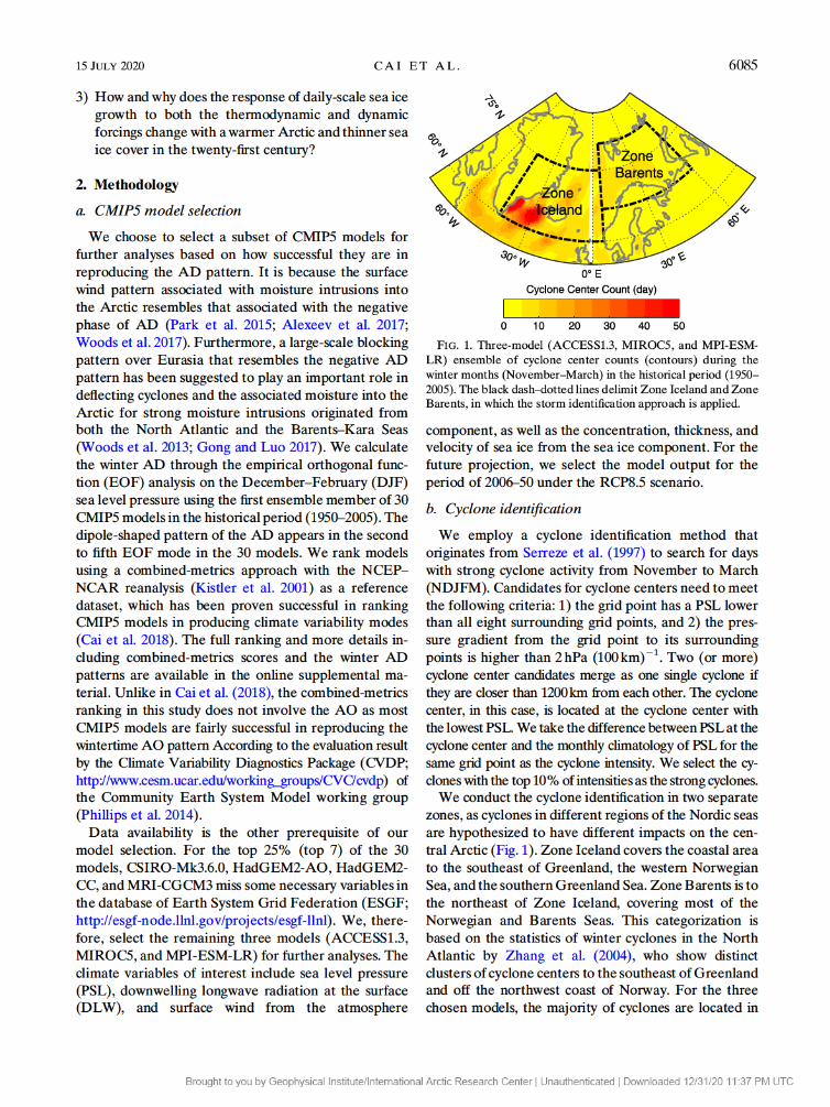
We conduct the cyclone identification in two separate
zones, as cyclones in different regions of the Nordic seas
are hypothesized to have different impacts on the cen-
tral Arctic (Fig. 1). Zone Iceland covers the coastal area
to the southeast of Greenland, the western Norwegian
Sea, and the southern Greenland Sea. Zone Barents is to
the northeast of Zone Iceland, covering most of the
Norwegian and Barents Seas. This categorization is
based on the statistics of winter cyclones in the North
Atlantic by Zhang et al. (2004), who show distinct
clusters of cyclone centers to the southeast of Greenland
and off the northwest coast of Norway. For the three
chosen models, the majority of cyclones are located in
FIG. 1. Three-model (ACCESS1.3, MIROC5, and MPI-ESM-
LR) ensemble of cyclone center counts (contours) during the
winter months (November–March) in the historical period (1950–
2005). The black dash–dotted lines delimit Zone Iceland and ZoneBarents, in which the storm identification approach is applied.
15 JULY2020 C A I E T A L . 6085
Brought to you by Geophysical Institute/International Arctic Research Center | Unauthenticated | Downloaded 12/31/20 11:37 PM UTC
Zone Iceland, although there are also substantial num-
bers of cyclones in Zone Barents (Fig. 1). The spatial
distribution of the models’ cyclone centers is generally
similar to that in observation and reanalysis datasets
(Zhang et al. 2004;Rudeva and Gulev 2011). We ex-
clude Greenland from cyclone identification, as its high
altitude could bring low pressure biases when extrapo-
lating surface pressure to sea level.
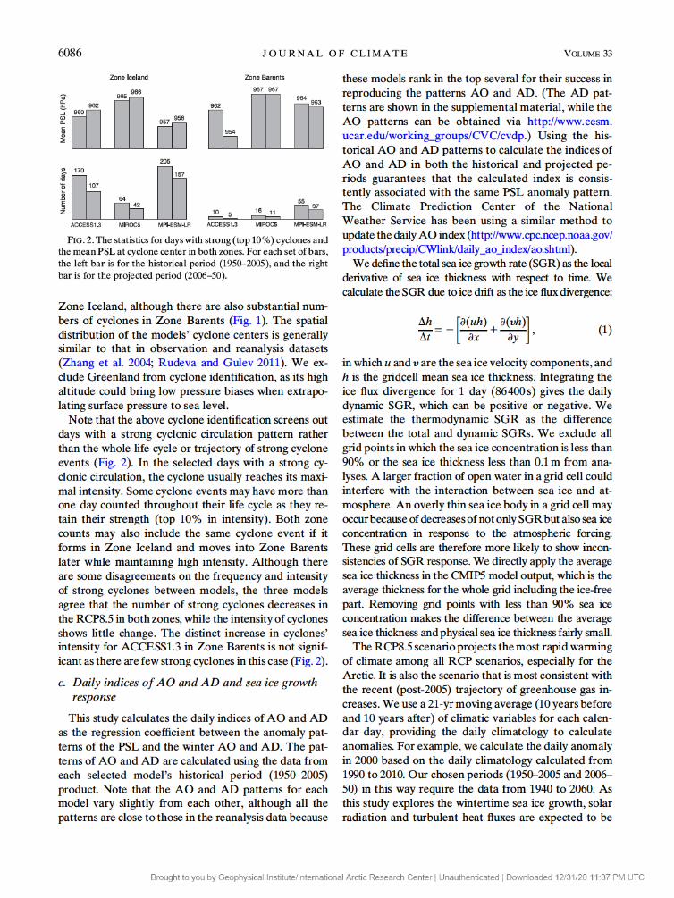
Note that the above cyclone identification screens out
days with a strong cyclonic circulation pattern rather
than the whole life cycle or trajectory of strong cyclone
events (Fig. 2). In the selected days with a strong cy-
clonic circulation, the cyclone usually reaches its maxi-
mal intensity. Some cyclone events may have more than
one day counted throughout their life cycle as they re-
tain their strength (top 10% in intensity). Both zone
counts may also include the same cyclone event if it
forms in Zone Iceland and moves into Zone Barents
later while maintaining high intensity. Although there
are some disagreements on the frequency and intensity
of strong cyclones between models, the three models
agree that the number of strong cyclones decreases in
the RCP8.5 in both zones, while the intensity of cyclones
shows little change. The distinct increase in cyclones’
intensity for ACCESS1.3 in Zone Barents is not signif-
icant as there are few strong cyclones in this case (Fig. 2).
c. Daily indices of AO and AD and sea ice growthresponse
This study calculates the daily indices of AO and AD
as the regression coefficient between the anomaly pat-
terns of the PSL and the winter AO and AD. The pat-
terns of AO and AD are calculated using the data from
each selected model’s historical period (1950–2005)
product. Note that the AO and AD patterns for each
model vary slightly from each other, although all the
patterns are close to those in the reanalysis data because
these models rank in the top several for their success in
reproducing the patterns AO and AD. (The AD pat-
terns are shown in the supplemental material, while the
AO patterns can be obtained via http://www.cesm.
ucar.edu/working_groups/CVC/cvdp.) Using the his-
torical AO and AD patterns to calculate the indices of
AO and AD in both the historical and projected pe-
riods guarantees that the calculated index is consis-
tently associated with the same PSL anomaly pattern.
The Climate Prediction Center of the National
Weather Service has been using a similar method to
update the daily AO index (http://www.cpc.ncep.noaa.gov/
products/precip/CWlink/daily_ao_index/ao.shtml).
Wedefinethetotalseaicegrowthrate(SGR)asthelocal
derivative of sea ice thickness with respect to time. We
calculate the SGR due to ice drift as the ice flux divergence:
Dh
Dt52
›(uh)
›x1›(yh)
›y, (1)
in whichuandyare the sea ice velocity components, and
his the gridcell mean sea ice thickness. Integrating the
ice flux divergence for 1 day (86 400 s) gives the daily
dynamic SGR, which can be positive or negative. We
estimate the thermodynamic SGR as the difference
between the total and dynamic SGRs. We exclude all
grid points in which the sea ice concentration is less than
90% or the sea ice thickness less than 0.1 m from ana-
lyses. A larger fraction of open water in a grid cell could
interfere with the interaction between sea ice and at-
mosphere. An overly thin sea ice body in a grid cell may
occur because of decreases of not only SGR but also sea ice
concentration in response to the atmospheric forcing.
These grid cells are therefore more likely to show incon-
sistencies of SGR response. We directly apply the average
sea ice thickness in the CMIP5 model output, which is the
average thickness for the whole grid including the ice-free
part. Removing grid points with less than 90% sea ice
concentration makes the difference between the average
sea ice thickness and physical sea ice thickness fairly small.
The RCP8.5 scenario projects the most rapid warming
of climate among all RCP scenarios, especially for the
Arctic. It is also the scenario that is most consistent with
the recent (post-2005) trajectory of greenhouse gas in-
creases. We use a 21-yr moving average (10 years before
and 10 years after) of climatic variables for each calen-
dar day, providing the daily climatology to calculate
anomalies. For example, we calculate the daily anomaly
in 2000 based on the daily climatology calculated from
1990 to 2010. Our chosen periods (1950–2005 and 2006–
50) in this way require the data from 1940 to 2060. As
this study explores the wintertime sea ice growth, solar
radiation and turbulent heat fluxes are expected to be
FIG. 2. The statistics for days with strong (top 10%) cyclones andthe mean PSL at cyclone center in both zones. For each set of bars,
the left bar is for the historical period (1950–2005), and the right
bar is for the projected period (2006–50).
6086 JOURNAL OF CLIMATE VOLUME33
Brought to you by Geophysical Institute/International Arctic Research Center | Unauthenticated | Downloaded 12/31/20 11:37 PM UTC
negligibly low for the Arctic (Serreze et al. 2007a). We,
therefore, use the DLW to approximate the thermody-
namic forcing from the atmosphere as in other previous
studies (e.g.,Park et al. 2015;Woods and Caballero
2016). We include the analysis of other energy fluxes, as
well as the residual of the surface energy budget, in the
supplemental material to prove the dominant effect of
the DLW in this study.
3. Results
a. Sea ice growth response to strong storms
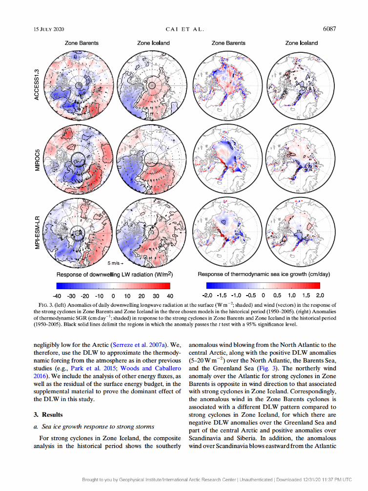
For strong cyclones in Zone Iceland, the composite
analysis in the historical period shows the southerly
anomalous wind blowing from the North Atlantic to the
central Arctic, along with the positive DLW anomalies
(5–20 W m22) over the North Atlantic, the Barents Sea,
and the Greenland Sea (Fig. 3). The northerly wind
anomaly over the Atlantic for strong cyclones in Zone
Barents is opposite in wind direction to that associated
with strong cyclones in Zone Iceland. Correspondingly,
the anomalous wind in the Zone Barents cyclones is
associated with a different DLW pattern compared to
strong cyclones in Zone Iceland, for which there are
negative DLW anomalies over the Greenland Sea and
part of the central Arctic and positive anomalies over
Scandinavia and Siberia. In addition, the anomalous
wind over Scandinavia blows eastward from the Atlantic
FIG. 3. (left) Anomalies of daily downwelling longwave radiation at the surface (W m22; shaded) and wind (vectors) in the response ofthe strong cyclones in Zone Barents and Zone Iceland in the three chosen models in the historical period (1950–2005). (right) Anomalies
of thermodynamic SGR (cm day21; shaded) in response to the strong cyclones in Zone Barents and Zone Iceland in the historical period
(1950–2005). Black solid lines delimit the regions in which the anomaly passes thettest with a 95% significance level.
15 JULY2020 C A I E T A L . 6087
Brought to you by Geophysical Institute/International Arctic Research Center | Unauthenticated | Downloaded 12/31/20 11:37 PM UTC

Ocean to eastern Europe. Considering that the Atlantic
water surface is warmer than the ambient land during
winter, such anomalous wind transports heat and mois-
ture and leads to positive DLW anomalies over eastern
Europe and Siberia, as well as some coastal regions in
the Arctic Ocean. The magnitude of the DLW anomaly
(5–20 W m22) is comparable to that from the strong
cyclones in Zone Iceland.
The spatial distributions of the daily thermodynamic
SGR anomaly generally match those of DLW in re-
sponse to strong cyclones in Zone Iceland (Fig. 3). The
greatest thermodynamic SGR inhibition (up to
2 cm day21) is in the Greenland and Barents Seas, ex-
tending to the central Arctic. For the strong cyclones in
Zone Barents, the thermodynamic SGR inhibition with
similar intensity (up to 2 cm day21) is in the Laptev and
East Siberian Seas for MIROC5, and in the Greenland
Sea and the Beaufort Sea for MPI-ESM-LR. In
ACCESS1.3 and MIROC5, the thermodynamic SGR
patterns for Zone Barents cyclones do not spatially
match the DLW pattern. The small sample sizes of
strong cyclonic days in these two models are partially
responsible for these differences (Fig. 2), considering
that most thermodynamic SGR inhibition in these cases
is not statistically significant. The calculation of ice flux
divergence could be inaccurate near the ice edge be-
cause of the discontinuity of the gridded ice concentra-
tions, causing biases to the calculation of dynamic and
thermodynamic SGRs. The biases cause the noisy signal
along the coast and the ice edge on the Atlantic side.
(See figures for the total SGR in the online supple-
mental material.)
The projections under the RCP8.5 scenario show a
warmer Arctic with thinner and smaller sea ice cover-
age. Over the polar cap (808N poleward), the abrupt
decrease of wintertime sea ice (NDJFM) thickness
starts around the 1990s in all three models (Fig. 4a).
The sea ice cover by 2050 is about 1.5 m thinner on
average compared to that in the 1990s. Meanwhile,
DLW over the polar cap increases at the rate of
2–3 W m22decade21(Fig. 4b). The mean sea ice area in
the Atlantic sector of the Arctic Ocean (608E–608W)
decreases, while the mean SST over the open-water area
in the North Atlantic (poleward of 608N) increases
(Figs. 4c,d). We detrend the time series in order to filter
out the long-term trend (global warming) and to em-
phasize interannual variability before calculating the
linear correlations. The linear correlation coefficients
for the detrended time series are negative between
DLW and sea ice area, and positive between DLW and
SST (Table 1). All linear correlations have at least a
93% significance level. The statistical significance of the
correlations suggests that a larger open-water area
with a warmer sea surface corresponds strongly with the
DLW increase in the central Arctic.
In the projection period, the composite analysis in
terms of strong cyclones shows similar DLW anomaly
FIG. 4. The time series of (a) sea ice thickness and (b) DLW
averaged over the polar cap (808–908N), and of (c) the area with sea
ice cover and (d) SST over the open water averaged over the Atlantic
sector of the Arctic Ocean (668–908N, 308E–608W), from Novemberto March in the years of 1950–2050 for the three chosen models.
6088 JOURNAL OF CLIMATE VOLUME33
Brought to you by Geophysical Institute/International Arctic Research Center | Unauthenticated | Downloaded 12/31/20 11:37 PM UTC
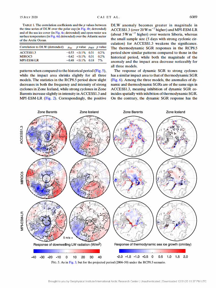
patterns when compared to the historical period (Fig. 5),
while the impact area shrinks slightly for all three
models. The statistics in the RCP8.5 period show slight
decreases in both the frequency and intensity of strong
cyclones in Zone Iceland, while strong cyclones in Zone
Barents increase slightly in intensity in ACCESS1.3 and
MPI-ESM-LR (Fig. 2). Correspondingly, the positive
DLW anomaly becomes greater in magnitude in
ACCESS1.3 (over 20 W m22higher) and MPI-ESM-LR
(about 5 W m22higher) over western Siberia, whereas
the small sample size (5 days with strong cyclonic cir-
culation) for ACCESS1.3 weakens the significance.
The thermodynamic SGR responses in the RCP8.5
period show similar patterns compared to those in the
historical period, while both the magnitude of the
anomaly and the impact area decrease noticeably for
all three models.
The response of dynamic SGR to strong cyclones
has a similar impact area to that of thermodynamic SGR
(Fig. 6). Among the three models, the anomalies of dy-
namic and thermodynamic SGRs are of the same sign in
ACCESS1.3, meaning inhibition of dynamic SGR co-
incides spatially with inhibition of thermodynamic SGR.
On the contrary, the dynamic SGR response has the
TABLE1. The correlation coefficients and thepvalues between
the time series of DLW over the polar cap (inFig. 4b; detrended)
and of the sea ice cover (inFig. 4c; detrended) and open-water sea
surface temperature (inFig. 4d; detrended) over the Atlantic sectorof the Arctic Ocean.
Correlation to DLW (detrended) rsic pvalue rSST pvalue
ACCESS1.3 20.53 ,0.1% 0.31 0.2%MIROC5 20.42 ,0.1% 0.31 0.2%
MPI-ESM-LR 20.48 ,0.1% 0.18 7%
FIG.5.AsinFig. 3, but for the projected period (2006–50) under the RCP8.5 scenario.
15 JULY2020 C A I E T A L . 6089
Brought to you by Geophysical Institute/International Arctic Research Center | Unauthenticated | Downloaded 12/31/20 11:37 PM UTC

opposite sign to the thermodynamic SGR response in
MIROC5 and MPI-ESM-LR, indicating that the dy-
namic and thermodynamic SGRs offset each other. The
differences in the spatial distribution of sea ice thickness
and anomalous wind between models lead to the dif-
ferences in the dynamic SGR responses among the
models. The absolute value of the dynamic SGR re-
sponse is smaller than that of the thermodynamic SGR
response in all cases.Park et al. (2015)have found the
stronger dynamic SGR response than thermodynamic
SGR response in the first few days of the arctic moisture
intrusion events. In comparison, the weaker dynamic
SGR response shown in this study is not in conflict, as
the cyclone identification in this study selects days with a
strong cyclonic circulation pattern, which usually occurs
days after the initial cyclone formation. In the RCP8.5
period, the dynamic SGR response also decreases rela-
tive to that in the historical period.
The decreased upward sensible heat flux at the surface
as warm and moist air blowing into the Arctic poten-
tially contributes to thermodynamic SGR inhibition. An
examination of the sensible heat flux response shows a
decreased upward sensible heat flux primarily in the sub-
Arctic regions, with little influence in the central Arctic
(see the figures in the supplemental material). We sug-
gest that the sensible heat flux decrease due to atmo-
spheric heat transport represents a partial contribution
to the thermodynamic SGR inhibition over the
FIG. 6. Anomalies of dynamic SGR (cm day21; shaded) in response to the strong cyclones in Zone Barents and Zone Iceland in the(left)
historical period (1950–2005) and (right) projected period (2006–50). Black solid lines delimit the regions in which the anomaly passes the
ttest with a 95% significance level.
6090 JOURNAL OF CLIMATE VOLUME33
Brought to you by Geophysical Institute/International Arctic Research Center | Unauthenticated | Downloaded 12/31/20 11:37 PM UTC

Greenland and Barents Seas, while increased DLW is
the dominant effect in the central Arctic Ocean to the
north of Svalbard.
b. Sea ice growth response to negative AD andpositive AO
The spatial distribution of daily DLW anomaly
regressed onto the negative AD (the AD index multi-
plied by21) is consistent with the response to the strong
cyclones in Zone Iceland (Fig. 7). The regressed DLW
(up to 30 W m22) and thermodynamic SGR (up to
2 cm day21) are largest in the Greenland and Barents
Seas, which expands poleward. The DLW regression
maps are similar between models, while the slightly
different anomalous wind corresponding to the slightly
different AD patterns alters the expansion direction of
the thermodynamic SGR toward the central Arctic in
the different models. Specifically, the regressed ther-
modynamic SGR inhibition in ACCESS1.3 expands
directly toward the North Pole, while that in MPI-ESM-
LR and MIROC5 expands toward northern Canada. For
other regions, three models agree on a reduction of the
thermodynamic SGR by up to 1 cm day21. The ther-
modynamic SGR regressed onto the negative AD has a
substantially larger impact area than that associated
with strong cyclones, as the negative AD corresponds to
the large-scale circulation pattern and wind anomaly.
We speculate that a combination of the strong Icelandic
low cyclonic circulation and a negative AD in the large-
scale circulation pattern would further enhance DLW
FIG. 7. (left) The map of daily DLW (W m22; shading) and wind (vectors) anomalies regressed onto the daily negative AD index in the
historical and RCP8.5 periods. (right) Anomalies of thermodynamic SGR (cm day21; shading) regressed onto the daily negative AD indexin the historical and the RCP8.5 periods.
15 JULY2020 C A I E T A L . 6091
Brought to you by Geophysical Institute/International Arctic Research Center | Unauthenticated | Downloaded 12/31/20 11:37 PM UTC

and thermodynamic SGR responses in the central
Arctic.
The magnitude of the thermodynamic SGR anomaly
regressed onto the negative AD is also noticeably
weaker with nearly unchanged DLW regression in the
RCP8.5 period than in the historical period (Fig. 7). In
ACCESS1.3, for example, the thermodynamic SGR in-
hibition in the RCP8.5 period is at least 0.5 cm day21less
than that in the historical period, and the impact area also
shrinks. Similar decreases are also present in MIROC5
and MPI-ESM-LR, with about 30%–60% reductions in
magnitude with smaller impact regions.
The DLW anomaly regressed on the positive AO
shows a pattern similar to the response to the strong
cyclones in Zone Barents (Fig. 8), but the smaller
magnitudes of the DLW regression correspond to
weaker (0.5 cm day21) thermodynamic SGR inhibition.
The thermodynamic SGR regressed on the positive AO
is also at least 50% weaker in magnitude compared to
that regressed on the negative AD. The spatial patterns
of DLW and thermodynamic SGR anomalies generally
match that a majority of the regions with positive DLW
anomalies are with negative thermodynamic SGR
anomalies. Exceptions are found over the coastal re-
gions of the Laptev Sea in MIROC5 and to the north of
Bering Strait in MPI-ESM-LR, for which the negative
anomalies of both the DLW and thermodynamic SGR
are very small. We suggest that the negative AD is more
important than the positive AO in atmospheric heat
transport from the Atlantic to the central Arctic.
Alexeev et al. (2017)have also argued that the process
of atmospheric heat import by Atlantic cyclones does
FIG.8.AsinFig. 7, but for the regression of the daily positive AO index.
6092 JOURNAL OF CLIMATE VOLUME33
Brought to you by Geophysical Institute/International Arctic Research Center | Unauthenticated | Downloaded 12/31/20 11:37 PM UTC

not link directly to the AO–NAO pattern (see figure
showing the composite PSL anomaly of the cyclones in
the supplemental material). In the RCP8.5 period, the
dampened sensitivity of thermodynamic SGR responses
to the AO keeps being apparent.
Both the positive AO and negative AD are associated
with the dynamic SGR, which is substantially weaker
than the thermodynamic SGR on the daily scale (Fig. 9).
The absolute value of regressed dynamic SGR is over
50% weaker than the regressed thermodynamic SGR
for all three models. Like in the composite analysis in
terms of strong cyclones, the regressed dynamic SGR in
ACCESS1.3 has the same sign as that of the regressed
thermodynamic SGR, while for the other models the
regressed dynamic and thermodynamic SGRs have
opposite signs. In the RCP8.5 period, the dynamic SGR
response is weaker in all three models.
c. Impact of a warmer Arctic on sea ice growth
The results described in the above sections consis-
tently show a dampened sensitivity of SGR in response
to different types of atmospheric forcing in the RCP8.5
period. Statistics over the polar cap show that the
5-month (NDJFM) total sea ice growth has an increas-
ing trend over the RCP8.5 period in all three models
(Fig. 10a), leading to higher sea ice production in the
warmer Arctic. Meanwhile, the standard deviation for
daily SGR during the five winter months decreases,
meaning that daily variability in SGR is smaller in the
RCP8.5 period (Fig. 10b).
FIG. 9. Anomalies of dynamic SGR (cm day21; shaded) regressed onto (left) positive AO and (right) negative AD in the historical period
(1950–2005) and projected period (2006–50).
15 JULY2020 C A I E T A L . 6093
Brought to you by Geophysical Institute/International Arctic Research Center | Unauthenticated | Downloaded 12/31/20 11:37 PM UTC

Focusing on the negative AD, we quantify its inhibi-
tion of sea ice growth thermodynamically each winter
over the polar cap by the following formula:
C5n
i51
(R3ADi), (2)
whereRis the regression coefficient between the daily
anomaly of thermodynamic SGR and the negative AD
index (shown inFig. 7), and ADiis theith ofnnegative
AD index in the 5-month period. A negative AD
reduces sea ice growth by up to 0.7 m at maximum from
November to March each year in the historical period,
with the average between 0.2 and 0.4 m (Fig. 10c). In the
RCP8.5 period, the three models show that the AD-
contributed sea ice growth inhibition decreases by at
least 0.1 m, with up to a 60% decrease in interannual
variability.
In winter when the atmospheric temperature is below
freezing, the sea ice acts as an insulation layer inhibiting
growth from its bottom, which is why thinner sea ice
cover typically results in less insulation and higher
winter sea ice production. Based on the empirical for-
mula fromAnderson (1961), we derive sea ice growth
rate as a monotonically decreasing function of the base
state sea ice thickness as a verification of the higher sea
ice production with the thinner sea ice cover (see
Fig. S20a in the online supplemental material). For more
complex sea ice models, the CCSM3 has modeled 0.2–
0.4 m more sea ice production under a doubled-CO2scenario (Bitz et al. 2006), comparable to the CMIP5
simulations in this study. In addition, thinner sea ice
grows faster than thicker ice, so the spatial heteroge-
neity of sea ice thickness is expected to decrease as
Arctic sea ice thickness decreases as the climate warms.
Assuming the unchanged sea ice velocity, the less-
varying sea ice thickness results in a smaller ice diver-
gence flux and, in turn, a smaller dynamic SGR change
in response to the strong cyclones and large-scale cir-
culations. (See the online supplemental material for the
change in the gradient of sea ice thickness.)
The numerical implementation of the thermodynam-
ically forced sea ice growth-rate change in the CICE4
model helps to further diagnose the physics of damp-
ened thermodynamic SGR response in the RCP8.5 pe-
riod (Hunke et al. 2010). CICE4 serves as the sea ice
component in ACCESS1.3 (Uotila and O’Farrell 2010),
and it is probably the best-documented sea ice model
among the sea ice modeling systems in CMIP5. In
CICE4, the governing equation for the thermodynamic
sea ice growing/melting is as follows:
qbotdh5(F
cb2F
bot)Dt, (3)
where in the case of sea ice growthqbotis the enthalpy of
the newly grown sea ice layer at the bottom, which is
approximately a constant with definite freezing tem-
perature and salinity of sea ice;dhis the change in sea ice
thickness withinDt; andFcbandFbotare, respectively,
the conductive heat flux and the net downward heat flux
from ice to ocean. In the condition of extra downward
energy fluxDFN21from the overlying sea ice layer or
from the atmosphere, the changeDFcbis dependent on
the specific heatciand the thicknesshNof theNth layer:
FIG. 10. Time series of (a) the total growth of sea ice and (b) the
standard deviation of the daily sea ice growth rate in the 5-monthperiod in each year in the three chosen models. Dashed lines vi-
sualize the trends. (c) Boxplot showing the statistics of negative
AD–contributed sea ice growth inhibition in the historical period
(left plot of each model) and the RCP8.5 period (right plot ofeach model).
6094 JOURNAL OF CLIMATE VOLUME33
Brought to you by Geophysical Institute/International Arctic Research Center | Unauthenticated | Downloaded 12/31/20 11:37 PM UTC
DFcb5KiN11
Dhi
DFN21
cirihN
, (4)
in whichKiN11is the thermal conductivity of the newly
grown sea ice layer (beneath theNth layer, at the bot-
tom) with the growth rate ofDhi(m s21). The newly
grown layer is the only layer that is in contact with
seawater, and the temperature of which is consistently at
the freezing point of seawater. The specific heatciis a
function of sea ice temperatureT(8C) and salinity
S(psu):
ci(T,S)5c
01L0mS
T2, (5)
in whichc0andL0are, respectively, the specific heat and
latent heat of fusion of the fresh sea ice at 08C, andmis a
salinity parameter. Note thatcimonotonically increases
with sea ice temperature.
Assuming a maximum sea ice salinity, the schematic
diagram of ice growth from the bottom in response to
every extra 1 W m22of downward radiation flux is de-
rived from the above equations. In response to the same
strength of extra heat flux acting on a certain thickness
of sea ice, the change in SGR is a monotonous de-
creasing function of sea ice temperature (see Fig. S20b).
In this way, we prove the reduced sensitivity of the
thermodynamic SGR response in the RCP8.5 period
from a physical point of view.
4. Discussion
The SGR responses to examined in this study suggests
a substantially (.50%) stronger thermodynamic SGR
response than dynamic SGR response on a daily scale
associated with both the positive AO and negative AD.
Note that what the SGR responses are associated with
is a strong daily AO–AD (one standard deviation) pat-
tern (Figs. 7and8). Compared to the previous study that
ice drift contributes a majority of sea ice thickness
change on the seasonal scale during positive AO winters
(Park et al. 2018), this study complements that for a
short period, the thermodynamic forcing is likely to
outweigh the dynamic forcing in inhibiting sea ice
growth if with a strong AO-like circulation pattern. In
addition, the daily negative AD is the greater contrib-
uting factor than the positive AO in thermodynamically
inhibiting daily sea ice growth, even though AO is the
dominant climatic variability mode over the Arctic. It
verifies our model ranking approach that prioritizes
models’ performance in reproducing AD in winter.
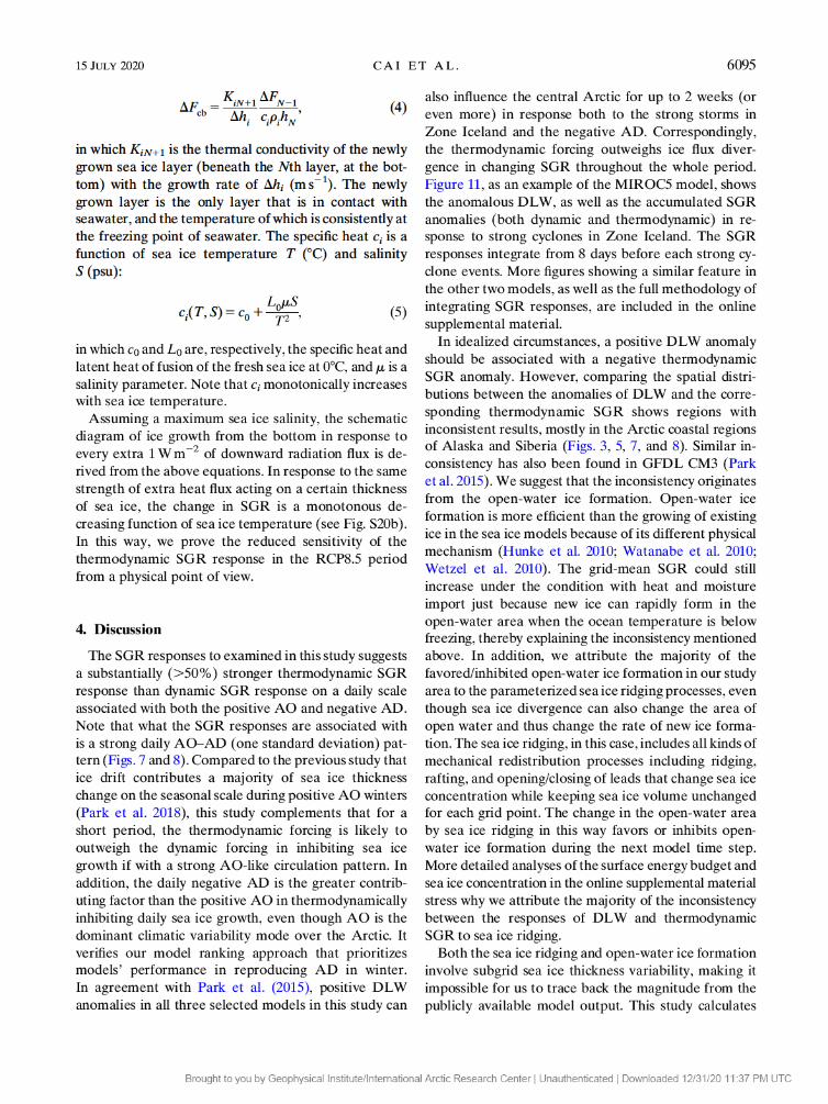
In agreement withPark et al. (2015), positive DLW
anomalies in all three selected models in this study can
also influence the central Arctic for up to 2 weeks (or
even more) in response both to the strong storms in
Zone Iceland and the negative AD. Correspondingly,
the thermodynamic forcing outweighs ice flux diver-
gence in changing SGR throughout the whole period.
Figure 11, as an example of the MIROC5 model, shows
the anomalous DLW, as well as the accumulated SGR
anomalies (both dynamic and thermodynamic) in re-
sponse to strong cyclones in Zone Iceland. The SGR
responses integrate from 8 days before each strong cy-
clone events. More figures showing a similar feature in
the other two models, as well as the full methodology of
integrating SGR responses, are included in the online
supplemental material.
In idealized circumstances, a positive DLW anomaly
should be associated with a negative thermodynamic
SGR anomaly. However, comparing the spatial distri-
butions between the anomalies of DLW and the corre-
sponding thermodynamic SGR shows regions with
inconsistent results, mostly in the Arctic coastal regions
of Alaska and Siberia (Figs. 3,5,7, and8). Similar in-
consistency has also been found in GFDL CM3 (Park
et al. 2015). We suggest that the inconsistency originates
from the open-water ice formation. Open-water ice
formation is more efficient than the growing of existing
ice in the sea ice models because of its different physical
mechanism (Hunke et al. 2010;Watanabe et al. 2010;
Wetzel et al. 2010). The grid-mean SGR could still
increase under the condition with heat and moisture
import just because new ice can rapidly form in the
open-water area when the ocean temperature is below
freezing, thereby explaining the inconsistency mentioned
above. In addition, we attribute the majority of the
favored/inhibited open-water ice formation in our study
area to the parameterized sea ice ridging processes, even
though sea ice divergence can also change the area of
open water and thus change the rate of new ice forma-
tion. The sea ice ridging, in this case, includes all kinds of
mechanical redistribution processes including ridging,
rafting, and opening/closing of leads that change sea ice
concentration while keeping sea ice volume unchanged
for each grid point. The change in the open-water area
by sea ice ridging in this way favors or inhibits open-
water ice formation during the next model time step.
More detailed analyses of the surface energy budget and
sea ice concentration in the online supplemental material
stress why we attribute the majority of the inconsistency
between the responses of DLW and thermodynamic
SGR to sea ice ridging.
Both the sea ice ridging and open-water ice formation
involve subgrid sea ice thickness variability, making it
impossible for us to trace back the magnitude from the
publicly available model output. This study calculates
15 JULY2020 C A I E T A L . 6095
Brought to you by Geophysical Institute/International Arctic Research Center | Unauthenticated | Downloaded 12/31/20 11:37 PM UTC
the thermodynamic SGR by subtracting the dynamic
SGR from the total SGR, therefore involving the SGR
change due to open-water ice formation as a bias in the
thermodynamic SGR. The numerical implementation of
ridging in these three models involves a fraction of the
thinnest sea ice (15% for CICE4 and MIROC5), and sea
ice ridging is more active between thinner than thicker
sea ice bodies (Bitz et al. 2001;Hunke et al. 2010).
During the growing season (November–April), most
CICE4-simulated ridging happens along the Arctic
coastal regions to the north of Alaska and Siberia, and
along the ice edge on the Atlantic side (Hunke 2010).
We, therefore, argue that for this study the bias of SGR
response due to the neglected ridging process is small in
the central Arctic (polar cap). Furthermore, excluding
all grid points with the sea ice concentration less than
90% or thickness less than 0.1 m from the analysis
eliminates some high-bias area along the ice edge on the
Atlantic side. The remaining high-bias regions due to
ridging are along the Arctic coast of Eurasia and Alaska,
in which we found the most inconsistency between the
anomalies of DLW and thermodynamic SGR.
CMIP5 models differ in their formulations of sea
ice physics and in the response of sea ice to a warming
climate (Massonnet et al. 2012). This study verifies
that slight differences between models in the anoma-
lous wind and spatial distribution of sea ice thickness
can result in a substantial diversity in dynamic SGR
FIG. 11. (left) Anomalous DLW and the accumulated (center) dynamic and (right) thermodynamic SGR
anomalies in response to strong cyclones in Zone Iceland with the lag time of (top) 0, (middle)14, and (bottom)18
days. Maps are made based on the data in the historical period (1950–2005) for the MIROC5 model. The accu-mulation of SGR responses is from 8 days before each strong cyclone event.
6096 JOURNAL OF CLIMATE VOLUME33
Brought to you by Geophysical Institute/International Arctic Research Center | Unauthenticated | Downloaded 12/31/20 11:37 PM UTC

responses. Compared to the results inPark et al. (2018)
based on GFDL CM3, ACCESS1.3 presents a similar
AO-driven dynamic SGR change pattern, while
MIROC5 and MPI-ESM-LR present more or less the
opposite patterns spatially. This result is consistent with
that inBoland et al. (2017)that the ensemble of all
CMIP5 models shows a weak linkage between Arctic
sea ice decline and AO. It is apparent that further
studies are necessary on how and why CMIP5 models
agree or disagree with each other in modeling Arctic sea
ice variability in response to atmospheric circulation
patterns.
The three models in this study, as well as all other
CMIP5 models, differ from each other in the simulated
frequency and intensity of cyclones in the Nordic seas.
CMIP5 models typically underestimate the frequency
and intensity of cyclones in the Norwegian Sea, and they
have systematic biases in modeling the frequency and
intensity of North Atlantic cyclones (Zappa et al. 2013).
However, these biases do not invalidate our conclusions,
as all three models demonstrate a plausible physical
relationship between the atmospheric forcing and sea
ice growth inhibition. High-frequency observations on
sea ice thickness and atmospheric variables would help
evaluate the disagreement between models. As the
number of available CMIP6 products keeps growing, a
similar analysis on CMIP6 model products could be in-
teresting for the same topic assuming their numerical
implementations for both the atmosphere and sea ice
are more advanced than the CMIP5 models (Eyring
et al. 2016).
In the RCP8.5 period, strong cyclones in Zone Iceland
result in slightly smaller DLW increases over the
central Arctic relative to the historical simulation. For
ACCESS1.3 and MPI-ESM-LR, on the other hand,
strong cyclones in Zone Iceland result in a slight in-
crease in positive DLW anomalies over western Siberia
and/or the Kara and Laptev Seas.Zappa et al. (2013)
have found that in the twenty-first century, the CMIP5-
modeled high-level (250-hPa) zonal wind speed is
stronger over a strip-shaped region along the North Sea,
the Baltic Sea, and western Siberia. Such a wind speed
increase implies a change in the jet stream pathways and
storm track locations that could favor extra heat and
moisture transporting to western Siberia and its Arctic
coastal region, which is consistent with our results in this
study. We, therefore, speculate that strong cyclones in
Zone Barents in the future could transport moisture and
heat from the Atlantic with a higher efficiency, which
impacts the regional climate and inhibits sea ice growth
in the Barents, Kara, and Laptev Seas. On the other
hand, the decrease in the frequency of cyclones for
both zones can possibly make the wintertime Atlantic
cyclone a less important contributing factor in affecting
sea ice growth and Arctic warming in the future.
5. Conclusions
This study explores daily Arctic sea ice growth under
the impact of winter cyclones in the Nordic Seas and
large-scale atmospheric circulation patterns. We select
ACCESS1.3, MIROC5, and MPI-ESM-LR from 30
CMIP5 models because of their superiority in repro-
ducing the winter AD in the historical period (1950–
2005) and data availability. A cyclone identification
method enables the selection of strong cyclones in two
separate regions in the Nordic seas. The total sea ice
growth rate (SGR) change is considered as the sum of
the growth rates due to ice drift (dynamic forcing) and
thermodynamic forcing, respectively.
Both strong cyclones and large-scale circulation pat-
terns can import atmospheric heat and moisture trans-
ports into the central Arctic, resulting in a positive
anomaly of downward longwave radiation (DLW) that
thermodynamically inhibits wintertime sea ice growth.
Both strong cyclones in Zone Iceland and the negative
AD can thermodynamically inhibit SGR in the
Greenland and Barents Seas, and the regions with in-
hibition are extended into the central Arctic by the
anomalous wind. Both strong cyclones in Zone Barents
and the positive AO inhibit the thermodynamic SGR
mostly along the Arctic coast of Siberia. The AO and
AD as large-scale circulation patterns lead to a wider
range of thermodynamic SGR inhibition than strong
Nordic seas cyclones do. Because the negative AD
causes stronger thermodynamic SGR inhibition in the
central Arctic than the positive AO, we consider the AD
as the more important mode of climatic variability
in thermodynamically inhibiting wintertime sea ice
growth. On the daily scale, the thermodynamic SGR
change consistently exceeds the dynamic SGR change in
response to strong cyclonic circulation and large-scale
circulation patterns over the Arctic, including the
AO and AD.
The three CMIP5 models in this study agree on a
dampened sensitivity of both dynamic and thermody-
namic SGR changes in response to strong cyclones
and large-scale circulation patterns in the RCP8.5
future projection period. As the Arctic warms, thinner
sea ice makes the insulation effect weaker, favoring sea
ice growth. The smaller and less spatially variable sea ice
thickness field decreases ice flux divergence, therefore
decreasing the dynamic SGR response. Meanwhile, a
warmer sea ice temperature increases the specific heat
of sea ice, weakening thermodynamic SGR change in
response to the same atmospheric heat input from
15 JULY2020 C A I E T A L . 6097
Brought to you by Geophysical Institute/International Arctic Research Center | Unauthenticated | Downloaded 12/31/20 11:37 PM UTC
above. We suggest that the short-term SGR change due
to daily-scale atmospheric forcing, including the anom-
alous wind pattern and enhanced downward longwave
radiation from the atmosphere, will play a less important
role in determining sea ice extent and thickness in the
warmer Arctic.
Acknowledgments.This publication is the result in
part of research sponsored by the Cooperative Institute
for Alaska Research with funds from the National
Oceanic and Atmospheric Administration (NOAA)
under Cooperative Agreement NA13OAR4320056
with the University of Alaska. V.A. was supported
by the Interdisciplinary Research for Arctic Coastal
Environments (InteRFACE) project through the
Department of Energy, Office of Science, Biological
and Environmental Research Program’s Regional
and Global Model Analysis program and by NOAA
project NA18OAR4590417. J.W. was supported by the
National Science Foundation Grant ARC-1602720, by
NOAA Grant NA17OAR4310160, and by the Office of
Naval Research Grant N000141812216. We thank Nate
Bauer for valuable comments on manuscript writing
and for doing proofreading.
REFERENCES
Alexeev, V. A., J. E. Walsh, V. V. Ivanov, V. A. Semenov, and
A. V. Smirnov, 2017: Warming in the Nordic Seas, North
Atlantic storms and thinning Arctic sea ice. Environ. Res.
Lett.,12, 084011,https://doi.org/10.1088/1748-9326/AA7A1D.Anderson, D. L., 1961: Growth rate of sea ice.J. Glaciol.,3, 1170–
1172,https://doi.org/10.1017/S0022143000017676.Bitz, C. M., M. M. Holland, A. J. Weaver, and M. Eby, 2001:
Simulating the ice-thickness distribution in a coupled climate
model. J. Geophys. Res.,106, 2441–2463,https://doi.org/
10.1029/1999JC000113.——, J. C. Fyfe, and G. M. Flato, 2002: Sea ice response to wind
forcing from AMIP models.J. Climate,15, 522–536,https://
doi.org/ 10.1175/1520-0442(2002)015,0522:SIRTWF.2.0.CO;2.——, P. R. Gent, R. A. Woodgate, M. M. Holland, and R. Lindsay,
2006: The influence of sea ice on ocean heat uptake in response to
increasing CO2.J. Climate,19, 2437–2450,https://doi.org/10.1175/
JCLI3756.1.Boisvert, L. N., A. A. Petty, and J. C. Stroeve, 2016: The impact of
the extreme winter 2015/16 Arctic cyclone on the Barents–
Kara Seas.Mon. Wea. Rev.,144, 4279–4287,https://doi.org/
10.1175/MWR-D-16-0234.1.
Boland, E. J. D., T. J. Bracegirdle, and E. F. Shuckburgh, 2017:
Assessment of sea ice–atmosphere links in CMIP5 models.Climate
Dyn.,49, 683–702,https://doi.org/10.1007/s00382-016-3367-1.
Cai, L., V. A. Alexeev, J. E. Walsh, and U. S. Bhatt, 2018: Patterns,
impacts, and future projections of summer variability in the
Arctic from CMIP5 models.J. Climate,31, 9815–9833,https://
doi.org/10.1175/JCLI-D-18-0119.1.
Deser, C., 2000: On the teleconnectivity of the ‘‘Arctic
Oscillation.’’ Geophys.Res.Lett.,27, 779–782,https://
doi.org/10.1029/1999GL010945.
Eyring, V., S. Bony, G. A. Meehl, C. A. Senior, B. Stevens, R. J.
Stouffer, and K. E. Taylor, 2016: Overview of the Coupled
Model Intercomparison Project Phase 6 (CMIP6) experi-
mental design and organization.Geosci. Model Dev.,9, 1937–
1958,https://doi.org/10.5194/gmd-9-1937-2016.
Gong, T., and D. Luo, 2017: Ural blocking as an amplifier of the
Arctic sea ice decline in winter.J. Climate,30, 2639–2654,
https://doi.org/10.1175/JCLI-D-16-0548.1.
Gulev, S. K., O. Zolina, and S. Grigoriev, 2001: Extratropical cy-
clone variability in the Northern Hemisphere winter from the
NCEP/NCAR reanalysis data. Climate Dyn.,17, 795–809,
https://doi.org/10.1007/s003820000145.
Hunke, E. C., 2010: Thickness sensitivities in the CICE sea ice
model. Ocean Modell.,34, 137–149,https://doi.org/10.1016/
j.ocemod.2010.05.004.
——, W. H. Lipscomb, A. K. Turner, N. Jeffery, and S. Elliott,
2010: CICE: The Los Alamos Sea Ice Model documentation
and software user’s manual version 4.1. Rep. LA-CC-06-012,
Los Alamos National Laboratory T-3 Fluid Dynamics Group, 76
pp.,https://csdms.colorado.edu/w/images/CICE_documentation_
and_software_user%27s_manual.pdf.
Kistler, R., and Coauthors, 2001: The NCEP–NCAR 50-year
Reanalysis: Monthly means CD-ROM and documentation.
Bull. Amer. Meteor. Soc.,82, 247–267,https://doi.org/10.1175/
1520-0477(2001)082,0247:TNNYRM.2.3.CO;2.Kwok, R., and D. A. Rothrock, 2009: Decline in Arctic sea ice
thickness from submarine and ICESat records: 1958–2008.
Geophys. Res. Lett.,36, L15501,https://doi.org/10.1029/
2009GL039035.
Lindsay, R., and A. Schweiger, 2015: Arctic sea ice thickness loss
determined using subsurface, aircraft, and satellite observa-
tions.Cryosphere,9, 269–283,https://doi.org/10.5194/tc-9-269-
2015.Maslanik, J. A., C. Fowler, J. Stroeve, S. Drobot, J. Zwally, D. Yi,
and W. Emery, 2007: A younger, thinner Arctic ice cover:
Increased potential for rapid, extensive sea-ice loss.Geophys.
Res. Lett.,34, L24501,https://doi.org/10.1029/2007GL032043.
Massonnet, F., T. Fichefet, H. Goosse, C. M. Bitz, G. Philippon-
Berthier, M. M. Holland, and P. Y. Barriat, 2012: Constraining
projections of summer Arctic sea ice.Cryosphere,6, 1383–
1394,https://doi.org/10.5194/tc-6-1383-2012.
Maykut, G. A., 1978: Energy exchange over young sea ice in the
central Arctic.J. Geophys. Res.,83, 3646–3658,https://doi.org/
10.1029/JC083iC07p03646.Mizuta, R., 2012: Intensification of extratropical cyclones associ-
ated with the polar jet change in the CMIP5 global warming
projections.Geophys. Res. Lett.,39, L19707,https://doi.org/
10.1029/2012GL053032.
NSIDC, 2018: Arctic winter warms up to a low summer ice season.
National Snow and Ice Data Center, accessed 2 November
2019,https://nsidc.org/arcticseaicenews/2018/05/arctic-winter-
warms-up-to-a-low-summer-ice-season/.
Park, H.-S., S. Lee, S.-W. Son, S. B. Feldstein, and Y. Kosaka, 2015:
The impact of poleward moisture and sensible heat flux on
Arctic winter sea ice variability.J. Climate,28, 5030–5040,
https://doi.org/10.1175/JCLI-D-15-0074.1.
——, A. L. Stewart, and J.-H. Son, 2018: Dynamic and thermo-
dynamic impacts of the winter Arctic Oscillation on summer
sea ice extent.J. Climate,31, 1483–1497,https://doi.org/
10.1175/JCLI-D-17-0067.1.
Phillips, A. S., C. Deser, and J. Fasullo, 2014: Evaluating modes of
variability in climate models,Eos Trans. Amer.Geophys.
Union,95, 453,https://doi.org/10.1002/2014EO490002.
6098 JOURNAL OF CLIMATE VOLUME33
Brought to you by Geophysical Institute/International Arctic Research Center | Unauthenticated | Downloaded 12/31/20 11:37 PM UTC

Rigor, I. G., J. M. Wallace, and R.L. Colony, 2002: Response of sea ice
to the Arctic Oscillation.J. Climate,15, 2648–2663,https://doi.org/
10.1175/1520-0442(2002)015,2648:ROSITT.2.0.CO;2.
Rogers, J. C., 1997: North Atlantic storm track variability and itsassociation to the North Atlantic Oscillation and climate
variability of northern Europe.J. Climate,10, 1635–1647,
https://doi.org/10.1175/1520-0442(1997)010,1635:NASTVA.
2.0.CO;2.Rudeva, I., and S. K. Gulev, 2011: Composite analysis of North
Atlantic extratropical cyclones in NCEP–NCAR reanalysis
data.Mon. Wea. Rev.,139, 1419–1446,https://doi.org/10.1175/
2010MWR3294.1.Serreze, M. C., and R. G. Barry, 1988: Synoptic activity in the
Arctic basin, 1979–85.J. Climate,1, 1276–1295,https://doi.org/
10.1175/1520-0442(1988)001,1276:SAITAB.2.0.CO;2.——, and J. Stroeve, 2015: Arctic sea ice trends, variability and
implications for seasonal ice forecasting.Philos. Trans. Roy.
Soc.,373A, 20140159,https://doi.org/10.1098/rsta.2014.0159.
——, F. Carse, R. G. Barry, and J. C. Rogers, 1997: Icelandic lowcyclone activity: Climatological features, linkages with the
NAO, and relationships with recent changes in the Northern
Hemisphere circulation.J. Climate,10, 453–464,https://doi.org/
10.1175/1520-0442(1997)010,0453:ILCACF.2.0.CO;2.——, A. P. Barrett, A. G. Slater, M. Steele, J. Zhang, and K. E.
Trenberth, 2007a: The large-scale energy budget of the Arctic.
J. Geophys. Res.,112, D11122,https://doi.org/10.1029/2006JD008230.
——, M. M. Holland, and J. Stroeve, 2007b: Perspectives on the
Arctic’s shrinking sea-ice cover. Science,315, 1533–1536,
https://doi.org/10.1126/science.1139426.Stroeve, J., M. Serreze, S. Drobot, S. Gearheard, M. Holland,
J. Maslanik, W. Meier, and T. Scambos, 2008: Arctic sea ice
extent plummets in 2007.Eos, Trans. Amer. Geophys. Union,
89, 13,https://doi.org/10.1029/2008EO020001.——, V. Kattsov, A. Barrett, M. Serreze, T. Pavlova, M. Holland,
and W. N. Meier, 2012: Trends in Arctic sea ice extent from
CMIP5, CMIP3 and observations.Geophys. Res. Lett.,39,L16502,https://doi.org/10.1029/2012GL052676.
——, A. Barrett, M. Serreze, and A. Schweiger, 2014: Using rec-
ords from submarine, aircraft and satellites to evaluate climate
model simulations of Arctic sea ice thickness.Cryosphere,8,1839–1854,https://doi.org/10.5194/tc-8-1839-2014.
Taylor, K. E., R. J. Stouffer, and G. A. Meehl, 2012: An overview of
CMIP5 and the experiment design.Bull. Amer. Meteor. Soc.,
93, 485–498,https://doi.org/10.1175/BAMS-D-11-00094.1.Thompson, D. W., and J. M. Wallace, 1998: The Arctic Oscillation
signature in the wintertime geopotential height and temper-
ature fields.Geophys. Res. Lett.,25, 1297–1300,https://doi.org/
10.1029/98GL00950.Tschudi, M., J. Stroeve, and J. Stewart, 2016: Relating the age of
Arctic sea ice to its thickness, as measured during NASA’s
ICESat and IceBridge campaigns.Remote Sens.,8, 457,https://
doi.org/10.3390/RS8060457.
Tsukernik, M., C. Deser, M. Alexander, and R. Tomas, 2010:
Atmospheric forcing of Fram Strait sea ice export: A closerlook.Climate Dyn.,35, 1349–1360,https://doi.org/10.1007/
s00382-009-0647-z.
Uotila, P., and S. O’Farrell, 2010: Sea ice in the ACCESS model.
CAWCR Tech. Rep. 033, 27–33,https://www.cawcr.gov.au/technical-reports/CTR_033.pdf.
Wadhams, P., and N. R. Davis, 2000: Further evidence of ice
thinning in the Arctic Ocean.Geophys. Res. Lett.,27, 3973–
3975,https://doi.org/10.1029/2000GL011802.Wang, M., and J. E. Overland, 2012: A sea ice free summer Arctic
within 30 years: An update from CMIP5 models.Geophys.
Res. Lett.,39, L18501,https://doi.org/10.1029/2012GL052868.Watanabe, M., and Coauthors, 2010: Improved climate simula-
tion by MIROC5: Mean states, variability, and climate sen-
sitivity.J. Climate,23, 6312–6335,https://doi.org/10.1175/
2010JCLI3679.1.Wei, J., X. Zhang, and Z. Wang, 2019: Impacts of extratropical
storm tracks on Arctic sea ice export through Fram Strait.
Climate Dyn.,52, 2235–2246,https://doi.org/10.1007/s00382-
018-4254-8.Wetzel, P., H. Haak, J. Jungclaus, and E. Maier-Reimer, 2010: The
Max-Planck-Institute global ocean/sea ice model with or-
thogonal curvilinear coordinates.Ocean Modell.,5, 91–127,https://doi.org/10.1016/S1463-5003(02)00015-X.
Woods, C., and R. Caballero, 2016: The role of moist intrusions in
winter Arctic warming and sea ice decline.J. Climate,29,
4473–4485,https://doi.org/10.1175/JCLI-D-15-0773.1.——, ——, and G. Svensson, 2013: Large-scale circulation associ-
ated with moisture intrusions into the Arctic during winter.
Geophys. Res. Lett.,40, 4717–4721,https://doi.org/10.1002/
grl.50912.——, ——, and ——, 2017: Representation of Arctic moist intru-
sions in CMIP5 models and implications for winter climate
biases.J. Climate,30, 4083–4102,https://doi.org/10.1175/JCLI-D-16-0710.1.
Yang, W., and G. Magnusdottir, 2018: Year-to-year variability in
Arctic minimum sea ice extent and its preconditions in ob-
servations and the CESM large ensemble simulations.Sci.Rep.,8, 9070,https://doi.org/10.1038/s41598-018-27149-y.
Zappa, G., L. C. Shaffrey, K. I. Hodges, P. G. Sansom, and D. B.
Stephenson, 2013: A multimodel assessment of future pro-
jections of North Atlantic and European extratropical cy-clones in the CMIP5 climate models.J. Climate,26, 5846–5862,
https://doi.org/10.1175/JCLI-D-12-00573.1.
Zhang, X., J. E. Walsh, J. Zhang, U. S. Bhatt, and M. Ikeda, 2004:
Climatology and interannual variability of Arctic cyclone ac-tivity: 1948–2002.J. Climate,17, 2300–2317,https://doi.org/
10.1175/1520-0442(2004)017,2300:CAIVOA.2.0.CO;2.
15 JULY2020 C A I E T A L . 6099
Brought to you by Geophysical Institute/International Arctic Research Center | Unauthenticated | Downloaded 12/31/20 11:37 PM UTC
Recommended