This document is downloaded from DR‑NTU (https://dr.ntu.edu.sg)Nanyang Technological University, Singapore.
Architecture‑intact oracle for fastest path andtime queries on dynamic spatial networks
Wei, Victor Junqiu; Wong, Raymond Chi‑Wing; Long, Cheng
2020
Wei, V. J., Wong, R. C. & Long, C. (2020). Architecture‑intact oracle for fastest path andtime queries on dynamic spatial networks. Proceedings of ACM SIGMOD InternationalConference on Management of Data, 1841‑1856.https://dx.doi.org/10.1145/3318464.3389718
https://hdl.handle.net/10356/148161
https://doi.org/10.1145/3318464.3389718
© 2020 Association for Computing Machinery (ACM). All rights reserved. This paper waspublished in Proceedings of ACM SIGMOD International Conference on Management of Dataand is made available with permission of Association for Computing Machinery (ACM).
Downloaded on 11 Nov 2021 19:00:45 SGT

Architecture-Intact Oracle for Fastest Path and TimeQueries on Dynamic Spatial Networks
Victor Junqiu Wei1, Raymond Chi-Wing Wong
2, Cheng Long
3
1Noah’s Ark Lab, Huawei Technologies,
2The Hong Kong University of Science and Technology,
3Nanyang Technological University
ABSTRACTGiven two vertices of interest (POIs) s and t on a spatial
network, a distance (path) query returns the shortest network
distance (shortest path) from s to t . This query has a variety
of applications in practice and is a fundamental operation
for many database and data mining algorithms.
In this paper, we propose an efficient distance and path
oracle on dynamic road networks using the randomization
technique. Our oracle has a good performance in practice and
remarkably, and at the same time, it has a favorable theoreti-
cal bound. Specifically, it has O(n log2 n) (resp. O(n log2 n))preprocessing time (resp. space) andO(log4 n log logn) (resp.O(log4 n log logn + l)) distance query time (resp. shortest
path query time) as well as O(log3 n) update time with high
probability (w.h.p.), where n is the number of vertices in the
spatial network and l is the number of edges on the shortest
path. Our experiments show that the existing oracles suffer
from a huge updating time that renders them impractical and
our oracle enjoys a negligible updating time and meanwhile
has comparable query time and indexing cost with the best
existing oracle.
ACM Reference Format: Victor JunqiuWei, Raymond Chi-Wing
Wong, Cheng Long. 2020. Architecture-Intact Oracle for Fastest
Path and TimeQueries onDynamic Spatial Networks. In Proceedingsof the 2020 ACM SIGMOD International Conference on Managementof Data (SIGMOD’20), June 14–19, 2020, Portland, OR, USA.. ACM,
NY, NY, USA, 16 pages. https://doi.org/10.1145/3318464.3389718
Permission to make digital or hard copies of all or part of this work for personal or classroom use is granted without fee provided that copies are not made or distributed for profit or commercial advantage and that copies bear this notice and the full citation on the first page. Copyrights for components of this work owned by others than ACM must be honored. Abstracting with credit is permitted. To copy otherwise, or republish, to post on servers or to redistribute to lists, requires prior specific permission and/or a fee. Request permissions from [email protected]. SIGMOD'20, June 14–19, 2020, Portland, OR, USA© 2020 Association for Computing Machinery.ACM ISBN 978-1-4503-6735-6/20/06…$15.00https://doi.org/10.1145/3318464.3389718
1 INTRODUCTIONWith the advance of GPS technology and the prevalence
of mobile devices, obtaining real-time spatial data becomes
increasingly popular, and many existing commercial compa-
nies such as “Google Maps” and “Bing Maps” are currently
using real-time spatial data for finding the fastest path from
a given source to a given destination. The fastest path is
computed based on a dynamic spatial network, where theweight associated to each edge could denote the travel time
on this edge and usually changes over time (due to the traffic
on this edge). Figure 1 shows a snapshot of a dynamic spatial
network, which is a directed graph with 8 vertices, namely
v1,v2, ...,v8, each denoting a spatial location and 10 edges
each denoting a road segment. In this snapshot, 3 edges have
their weights = 2 and the other edges have their weights = 1.
Let n be the total number of vertices in the spatial network.
The fastest path and the shortest travel time from a given
source to a given destination on a dynamic spatial network
could be regarded as the shortest path and the shortest dis-
tance when the weight of each edge is regarded as “distance”
instead of “travel time”. In the following, we refer them as
“shortest path” and “shortest distance”.
Computing the shortest path and the shortest distance
from a source to a destination on a dynamic spatial network
is very important. The reason is that there are a lot of appli-
cations starting from traditional drivers’ navigation, which
“aids” drivers to find a path, to recent autonomous car nav-
igation, which “completely control” unmanned vehicles to
move on the road. Besides, computing them efficiently is
very important in some real-life applications. One example
is emergency applications like delivering ambulances and
fire engines to target areas. In Hong Kong, it is expected that
ambulances arrive to target areas within about 12 minutes
[5]. Another example is time-critical applications in which
business people and travel salesmen with their own tight
schedule would prefer their travel schedule as fast as possible
without any delay. Furthermore, “shortest path/distance” is a
fundamental operator of many spatial queries, such as near-
est neighbor queries, range queries and spatial join queries,
and is also used in many scientific simulations [12, 33, 47].

v1
v2
v3
v4
v5
v6
v7
v8
1
2 1
11
11
1
2
2
Figure 1: An Example of A Spatial NetworkReturning the shortest path and the shortest distance effi-
ciently based on a dynamic spatial network is very challeng-
ing. Firstly, re-computing the shortest path and the shortest
distance from scratch is very costly whenever the weight of
an edge in the spatial network is updated. A straightforward
implementation is to execute the Dijkstra’s algorithm [27]
based on the current snapshot of the spatial network and
obtain the shortest path/distance whenever there is a weight
update. Although it is simple to implement, it is still slow
and does not return a result efficiently.
Secondly, existing algorithms [7, 8, 13, 29, 31, 38, 50–55, 63]
originally designed for finding the shortest path/distance
on a static spatial network, only one snapshot of a spatial
network, pre-compute some results in the form of index
(called oracle) and return the shortest path/distance effi-
ciently. But, they do not support the update operation on
the pre-computed results due to weight update. Thus, they
could not be used efficiently in the dynamic spatial network
setting. A straightforward adaptation of these algorithms
for the dynamic network setting is to re-construct the pre-
computed results from scratch whenever there is a weight
update. Then, each shortest path/distance query could be
answered based on the re-constructed pre-computed results.
Since the re-construction time complexities of these algo-
rithms are worse than O(n1.5), they are not efficient enough
for handling shortest path/distance queries [61, 63].
Thirdly, there are existing algorithms [26, 30, 56] proposed
for answering shortest path/distance queries on a dynamic
spatial network each of which also constructs an index/oracle
for answering shortest path/distance queries efficiently. But,
for the sake of maintaining the index/oracle due to theweight
update on the dynamic spatial network, the empirical update
time of each of these algorithms is still large. Even if some
of the algorithms have theoretical upper/lower bounds on
update time complexities, the lower bounds are also at least
linear to the number of vertices in the network. In practice,
the number of vertices is very large. Thus, those algorithms
are not scalable to the large spatial network.
Motivated by this, in this paper, we propose an oracle
called Update Efficient (UE) that has a short update time
and has a poly-logarithmic update time complexity, the first
best-known result. Besides, this oracle returns the shortest
path/distance efficiently. The key idea of the update effi-
ciency of UE is to keep the architecture (or structure) of UEunchanged (or intact) for any weight update on the dynamic
spatial network. All existing oracles require to perform a
time-consuming operation of updating/adjusting the archi-
tectures of their oracles for any weight update. The reason is
that the architecture of UE is dependent on only the original
graph/network structure (without the weight information)
and the initial randomly assigned ordering on vertices on
the graph/network. These remain unchanged for any weight
update. In contrast, the architecture of existing oracles in the
literature is dependent on the changing weight of any edge
on the spatial network. We will elaborate more in Section 4.
We summarize our major contributions as follows. Firstly,
we propose a novel oracle called UE that answers shortest
path/distance queries efficiently. Secondly, the time com-
plexity of updating our oracle is O(log3 n). This is the firstbest-known theoretical result since the existing best-known
worst-case update time complexity is at least O(n1.5) and the
existing best-known lower bound on the update time com-
plexity of the existing oracles is at least Ω(n). Thirdly, ourempirical study shows that the update time of all existing
oracles are too large, which could not be used in practice,
but the update time of our oracle is very small. In particular,
most existing oracles need to take more than one week for
weight update, and the update time of our oracle (which is
at most 50ms) is several orders of magnitude shorter than
that of the best-known oracle on all networks tested.
The remainder of the paper is organized as follows. Sec-
tion 2 defines the problem and Section 3 gives the related
work. Section 4 presents our distance oracle. Section 5 shows
our experimental results and Section 6 concludes our work.
2 PROBLEM DEFINITIONConsider a spatial network G(V ,E), where V is a set of all
vertices and E is a set of all edges on the network. Let n = |V |and m = |E |. Each directed edge (u,v) ∈ E in G has its
origin u and its destination v . Besides, it is associated with
its weight, denoted by wG (u,v), which changes over time.
Given a networkG(V ,E) and a vertex u ∈ V , we define theset of in-neighbors ofu, denoted by N in
G (u), to be the set of allvertices that are involved in edges in E with destinations as
u. That is, N inG (u) = v ∈ V |(v,u) ∈ E. Similarly, we define
the set of out-neighbors of u, denoted by N outG (u) to be the
set of all vertices that are involved in edges in E with origins
as u. That is, N outG (u) = v ∈ V |(u,v) ∈ E. In this paper, we
assume that there is no isolated vertex (i.e., for each u ∈ V ,N inG (u) ∪ N out
G (u) , ∅).Given two vertices, namely s and t , in V , we define a
path from s to t in the form of a list of vertices, namely
(v1,v2, ...,vl ), such that v1 = s , vl = t and for each
i ∈ [1, l − 1], (vi ,vi+1) ∈ E. Given a path π in the form
of (v1,v2, ...,vl ), we define the weight or the length of π to
be
∑l−1i=1wG (vi ,vi+1).

In the above, we represent the path in the form of a list of
vertices, says (v1,v2, ...,vl ), where (vi ,vi+1) ∈ E. We could
also represent the path as a list of consecutive edges in the
form of (v1,v2)·(v2,v3)·...·(vl−1,vl ).We call all vertices along
this path that are not a source vertex and are not a destination
vertex as passing vertices. In this example, v2,v3, ...,vl−1 arepassing vertices but v1 and vl are not.Given a path π from a vertex s to another vertex t in V ,
π is said to be the shortest path from s to t in network G,denoted by s ↣G t , if the length of π is the smallest among
all possible paths from s to t in G. Similarly, the shortestdistance from s to t in network G, denoted by dG (s, t), isdefined to be the length of s ↣G t . Note that the triangleinequality holds under function dG (·, ·).
Problem 1 (Oracle). We would like to design an oracleO that supports a short update time, and at the same time,answers any shortest path/distance query efficiently.
In the case when there are multiple shortest paths from sto t , the shortest path query studied in this paper only finds
an arbitrary shortest path among them. Thus, in the rest of
this paper, the term ‘shortest path from s to t ’ or ‘s-t shortestpath’ refers to an arbitrary shortest path from s to t .In this paper, we just focus on studying the case when
the weights of edges change over time. We do not consider
the case when new vertices and new edges are added. The
reason is that re-constructing the whole oracle from scratch
is already enough. Specifically, this case means that new
junctions and new road segments have to be built, which
may take more than several weeks and even several years [6].
Since in our experimental results, each oracle could be built
within one day, it is sufficient to rebuild the oracle from
scratch in this case. Furthermore, we do not discuss the case
when vertices and edges are removed. The reason is that this
case refers to our case that the weights of the corresponding
edges are updated to a very large value [28, 35, 49].
3 RELATEDWORKIn this section, we first present the related work on static
spatial networks (Section 3.1) and dynamic spatial networks(Section 3.2). Then, we describe some other studies that are
related to our study in Section 3.3.
3.1 Oracle on Static Spatial NetworksThere are a lot of existing studies about pre-computing
oracles on static spatial networks. We categorize them
into the following 7 categories: (1) partition-based ap-proaches [37, 38], (2) landmark-based approaches [31], (3)spatial coherence-based approaches [50, 55], (4) transit vertex-based approaches [8, 13, 14, 61], (5) 2-hop labeling ap-proaches [7, 10, 21, 36], (6) hierarchy-based approaches [29, 51,
52, 63], and (7) a hybrid approach [46], namely Hierarchical2-Hop Index (H2H in short).The partition-based approaches and landmark-based ap-
proaches are heuristic-based approaches without theoretical
guarantee. For spatial coherence-based approaches, there are
two representative algorithms under this category with theo-
retical bounds, namely Spatially Induced Linkage Cognizance(SILC) [50] and Path-Coherent Pair Decomposition (PCPD) [55].For transit vertex-based approaches, one representative algo-
rithm with theoretical bounds is called Transit Vertex Variant(TVV) [8]. For 2-hop labeling approaches, one representative
algorithm is called Pruned Landmark Labeling (PLL) [10]. Forhierarchy-based approaches, there are three representative
approaches, namely the Contraction Hierarchy (CH) [29], theHighway Hierarchy (HH) [51, 52] and the Arterial Hierarchy(AH) [63]. The experiments of [9] show that CH performs bet-
ter than PLL in terms of pre-computation time and space. For
the Hierarchical 2-Hop Index (H2H in short), this algorithm
combines the 2-hop labeling approach and the hierarchy-basedapproach. This combination significantly reduces the time
of finding labels in the 2-hop approach (used for finding
the shortest distance) with the help of the hierarchy-based
approach for a shortest distance query.
Although all of the above approaches were originally de-
signed for shortest path/distance queries in the static spatial
network setting (not the dynamic setting), we would like to
adapt some of the approaches/oracles in the dynamic set-
ting. Following [63], we consider adapting only oracles with
theoretical analysis. The reason is that in the experimental
results of [11, 34, 46, 61, 63], oracles with theoretical analysis
out-perform all oracles without theoretical analysis (includ-
ing the partition-based approaches and the landmark-based
approaches). Notice that in this section, we compare adapted
existing oracles with our oracle in theory and thus, only
consider the oracles with theoretical bounds. But, in the ex-
perimental section, we compared many other algorithms
without theoretical bounds. In this paper, we adapt five ora-
cles, namely SILC, PCPD, TVV, AH and H2H, to handle the
dynamic setting, and call them as SILC-Adapt, PCPD-Adapt,
TVV-Adapt, AH-Adapt and H2H-Adapt. It is not difficult to
adapt these oracles, and details of these adaptions could be
found in [59]. Table 1 shows a summary of these adapted
oracles in terms of preprocessing time, space, shortest dis-
tance query time, shortest path query time and update time.
In this table, the first five rows correspond to these 5 adapted
oracles. Notice that the update time complexity of each of
these oracles is at least O(n1.5). Besides, [59] shows that thelower bound of the update time complexity of each of these
oracles is Ω(n), which means that each of these oracles is
not scalable to a large network since n could be very large.
Note that although PLL and CH (designed for the static
version) described above have theoretical bounds, we did not

Table 1: Comparison of Distance and Path Oracles on Dynamic Spatial NetworksOracle Preprocessing Time Space Distance Query Time Shortest Path Query Time Update Time
SILC-Adapt [50] O (n2logn) O (n
√n) O (l logn) O (l logn) O (n2
logn)PCPD-Adapt [55] O (n2
logn) O (s3 · n) O (l logn) O (l logn) O (n2logn)
TVV-Adapt [8] O (n2logn logα ) O (Λn logn logα ) O (Λ2
log2 n log
2 α ) O (Λ2log
2 n log2 α + l ) O (n2
logn logα )AH-Adapt [63] O (hn2λ2) O (hnλ2) O (hλ2 logh + hλ4) O (hλ2 logh + hλ4 + l ) O (hn2λ2)H2H-Adapt [46] O (n1.5) O (n) O (
√n) O (l ·
√n) O (n1.5)
Dynamic-CH [26, 30] O (n2logn) O (n2) O (
√n logn) O (
√n logn + l ) O (n2
logn)Dynamic-PLL [11] O (n2
log2 n) O (n
√n logn) O (
√n logn) O (l
√n logn) O (n2
log3 n)
this paper O (n log2 n) w.h.p. O (n log
2 n) w.h.p. O (log4 n log logn) w.h.p. O (log4 n log logn + l ) w.h.p. O (log3 n) w.h.p.
Remark: l is the number of edges in the shortest path. h (resp. λ) is the height of the hierarchy that is equal to log
maxu,v∈V dG (u,v )minu,v∈V dG (u,v )
(resp. the Arterial Dimension of the spatial
networks) and they are proposed in [63]. h (resp. λ) is at most 26 (resp. 100) in the datasets tested in [63]. α is defined to be
maxu,v∈V dG (u,v )minu,v∈V dG (u,v )
. λ and Λ are all Ω(√n) in a grid
spatial network like that in Manhattan District. Note that the complexities of some of the above oracles rely on a feature, namely tree width, of the spatial network. It is shown in
[2] that the tree width of a spatial network is is as large as
√n in a square grid spatial network that is common in Manhattan district. Thus, we simply treat tree width as O (
√n)
in this paper. s is around 12 in practice.
adapt them because these two oracles were already adapted
by some existing papers and will be described in the next
section. Note that those of the 2-hop labeling approaches
other than PLL, though with theoretical bounds, are not
shown since they are significantly outperformed by PLL as
shown in the experiments of [10].
3.2 Oracles on Dynamic Spatial NetworksRecently, there are studies about pre-computing oracles on
dynamic spatial networks. There are four representative or-
acles. The first oracle is the dynamic version of oracle HH
called Dynamic-HH [56]. But, there is no theoretical bound
on Dynamic-HH. The second oracle is the dynamic version
of oracle CH called Dynamic-CH [26, 30]. The experimen-
tal results of [26, 30] show that Dynamic-CH outperforms
Dynamic-HH in terms of preprocessing time, space consump-
tion, query time and update time. The third oracle is the
dynamic version of oracle PLL called Dynamic-PLL [11]. The
fourth oracle is a bit parallel shortest path tree indexing struc-ture (BPL) [34] that is an indexing structure of answering
shortest path/distance queries on a dynamic network. It dy-
namically maintains several shortest path trees rooted at a
number of high-degree nodes. The query algorithm is a bi-
Dijkstra’s algorithm enhanced with some pruning operations
based on the information of the shortest path trees. It has
good empirical performance but has no theoretical analysis.
Note that among four oracles described above, only
Dynamic-CH and Dynamic-PLL have theoretical bounds. Ta-
ble 1 shows a summary about the complexities of these two
oracles, Dynamic-CH and Dynamic-PLL, where the third-to-
last and second-to-last rows correspond to these two oracles.
3.3 Some Other Related StudiesThere are some other studies related to our problem although
they are not exactly our problem. The first branch of related
studies is shortest path/distance queries on a time-dependentspatial network [15, 24, 39, 45, 57, 58, 62]. In these studies,
edge weights follow a pre-defined function that takes time as
input and returns a value (e.g., traffic) as output. This is un-
realistic in real world with “unexpected” events. The second
branch of related studies is approximate oracles on a dynamic
spatial network [53–55]. An approximate oracle returns an
approximate distance/path for each shortest distance/path
query but our oracle returns an exact distance/path. Thethird branch of related studies is Distance Sensitivity Ora-cle [18, 19, 44, 48, 60] that answers the shortest path/distancequeries with vertex/edge failures on static networks (not
dynamic networks studied in this paper).
4 DISTANCE AND PATH ORACLEIn this section, we describe our distance and path oracle
called the update-efficient (UE) oracle. Specifically, in Sec-
tion 4.1, we first give an important property called the
architecture-intact property, which is the key to the efficient
update time of UE and could not be satisfied by most (if not
all) existing oracles. Then, we describe our UE oracle in Sec-
tion 4.2. Next, we present the algorithms for preprocessing,
shortest distance/path query processing and update process-
ing in Section 4.3, Section 4.4 and Section 4.5, respectively.
Section 4.6 presents the theoretical analysis of our oracle.
4.1 Concept: Architecture-Intact PropertyGiven a data structure, the architecture of this data structureis defined to be a set of all components in this data structure
excluding all non-structural information (e.g., the weight
information). Different data structures have different defini-
tions of “architecture”. For example, consider a data structure
S that is a weighted graph containing 3 components, namely
V , E andW .V is a set of vertices, E is a set of directed edges
andW is a set of numbers each of which denotes the weight
of an edge in E. Here, each vertex in V could be regarded as
a sub-component of V and each edge in E could be regarded
as a sub-component of E. The architecture of this data struc-ture S is equal to the un-weighted graph containing V and
E only. Consider another example. The data structure used
in Dynamic-CH [26, 30] is a spatial network/graph inserted

with additional edges called shortcuts, where each edge is as-
sociated with a weight. Note that in Dynamic-CH, a shortcutfrom a vertex u to a vertex v is defined to be a new edge that
denotes/corresponds to the shortest path from u to v and its
weight is defined to the length of the corresponding path.
The architecture of this data structure is the un-weighted
version of the spatial network/graph inserted with additional
edges, where there is no weight associated to each edge. Con-
sider the third example. The data structure used in BPL [34]
is a set of (shortest path) trees, where each edge in the tree is
associated with a weight. The architecture of this data struc-
ture is the same set of trees but there is no weight associated
to each edge in the trees.
With the concept of “architecture”, we are ready to present
themajor results of our oracleUE.UE satisfies one interestingproperty called the architecture-intact property, which is the
key of an efficient update of our oracle. Specifically, we say
that an oracle constructed from a spatial network satisfies
the architecture-intact property if the architecture of the datastructure used in this oracle remains unchanged even when
there is an update on the weight of an edge in the spatial
network. Whenever there is a weight update, we just need
to update the non-structural information (e.g., the weight
information) in our oracle UE without updating the architec-
ture of the data structure. Updating the weight information
could be done efficiently since UE stores a mapping table
that could help to efficiently find a set of sub-components to
be updated for each edge if its associated weight is updated.
In our technical report [59], we show that most (if not all)
adapted algorithms originally designed for static spatial net-
works (in Section 3.1) do not satisfy the architecture-intact
property. The same is true for all algorithms originally de-
signed for dynamic spatial networks (in Section 3.2), i.e.,
they do not satisfy the architecture-intact property. This
explains why our oracle UE has a shorter update time com-
pared with existing algorithms. For example, in Dynamic-CH,when there is a weight update, some new shortcuts have to
be added to the architecture of the data structure used in
Dynamic-CH. Besides, in BPL, when there is a weight update,
some edges in the trees are removed and some other new
edges are inserted into the trees. Besides, this observation
is verified in our experimental results that most existing or-
acles need to take more than one week for weight update,
and the update time of our UE oracle (which is at most 50ms)
is several orders of magnitude shorter than that of the best-
known oracle on real-life datasets. More importantly, none
of the existing oracles can handle the update before the next
batch of update arrives in our experimental results.
The reason why a data structure that does not satisfy
the architecture-intact property has a larger update time is
that for any weight update, it has to perform a costly searchoperation on which components in the data structure should
have some new sub-components to be added and should
have some existing sub-components to be removed.
Let us give some details of our oracle UE to give the major
key idea why UE satisfies the architecture-intact property.
The idea is based on the novel definition of “shortcut” used in
UE that is independent of any update on theweight of an edgein the spatial network. That is, UE does not need to add or
remove any shortcuts in the network even though there is an
update on the weight of an edge in the network. To the best
of our knowledge, we are the first to give a “nice” definition
of “shortcut” such that there is no need to introduce any
insertion/deletion of “shortcut” for any edge-weight update.
Existing studies gave other definitions of “shortcut” that may
introduce potential insertion/deletion of “shortcut” for any
edge-weight update.
4.2 Our Oracle: UESpecifically, UE involves three components, namely the UEspatial graph, theweight mapping table and the occupant map-ping table. The UE spatial graph is an un-weighted graph that
is exactly equal to the un-weighted version of the original
graphG but there are additional edges in the UE spatial graph
compared with the original graph G. The weight mapping
table contains all the weight information about the edges in
the UE spatial graph. Specifically, it is a set of entries each
in the form of ((u,v),w), where (u,v) is an edge in the UE
spatial graphG ′ andw is the weight of (u,v) in graphG ′ (i.e.,wG′(u,v)). Here, although G
′is un-weighted, for the ease of
description, when we write “the weight of an edge inG ′”, wemean that there is a value called the weight associated to thisedge in the weight mapping table. The occupant mapping
table contains all the information about a new concept called
“occupant”, which will be described later. The occupant map-
ping table is a set of entries each in the form of ((u,v),o),where (u,v) is an edge in the UE spatial graph G ′ and o is avertex in V called the occupant of (u,v). Intuitively, UE uses
additional edges called shortcuts with the help of the weight
mapping table and the occupant mapping table to answer
shortest distance/path queries efficiently.
Before we define “shortcuts”, we first define the con-
cept of “rank” and then the concept of “valley path”. Ini-
tially, we perform Knuth shuffle [41] to obtain a random
ordering/permutation I of vertices in V . With this order-
ing/permutation I , the rank value of each vertex v in V ,denoted by RI (v), is defined to be its position of this order-
ing/permutation. Consider our running example containing
8 vertices as shown in Figure 1. Let the permutation I be(v1,v2,v3,v4,v5,v6,v7,v8). The rank value ofv1 (i.e., RI (v1))is equal to 1. The rank value of v2 (i.e., RI (v2)) is equal to 2.
A path (v1,v2, ...,vl ) is said to be a valley path if the rank
value of each vertex along the path except the first vertex v1

and the last vertex vl is smaller than both the rank values
of v1 and vl (i.e., each vertex along this path except s and thas its rank value smaller than minRI (s),RI (t)). The rea-son why we call this path as a “valley path” is described as
follows. In our terminology, we “interpret” that each vertex
could be associated with a location on a mountain with a
height. If the vertex has a larger rank value, it has a greater
height. According to this interpretation, all vertices along
the path except the first vertex and the last vertex have their
smaller heights, which looks like a “valley”. Notice that as a
special case, when a path from s to t contains exactly two
vertices (i.e., the path is (s, t)), this path is also a valley path.
Consider our running example in Figure 1, where permuta-
tion I is (v1,v2,v3,v4,v5,v6,v7,v8). Path (v5,v4,v3,v7) is avalley path since both the rank values ofv4 andv3 are smaller
than 5 (= minRI (v5),RI (v7)). Path (v5,v7) is also a valley
path since it contains exactly two vertices. Path (v5,v8,v7)is not a valley path because the rank value of v8 is greaterthan 5 (= minRI (v5),RI (v7)).
Besides, we denote the shortest valley path from s to t underthe permutation I by s I
G t . If the context of permutation is
clear, we simply denote it by u G v . Consider our runningexample. Path (v5,v7) is the shortest valley path from v5 tov7. Thus,v5
IG v7 = (v5,v7). But, path (v5,v4,v3,v7) is not
the shortest valley path from v5 to v7 since there exists apath from v5 to v7 (i.e., (v5,v7)), which has a smaller length.
In the following, when we write “u G v \ u,v”, we mean
the corresponding path excluding vertices u and v .Given two vertices, namely u and v , a shortcut from u
to v is defined to be an edge from u to v in G ′ denotingthe shortest valley path from u to v on the original spatialnetwork G. The weight of a shortcut is defined to be the
length of the corresponding path in G.UE keeps a certain number of shortcuts in the UE spatial
network such that it maintains the following property called
the shortcut property from time to time (e.g., even after there
is an edge weight update). This property is the major key to
the efficient update time of UE.
Property 1 (Shortcut Property). For each pair of ver-tices, namely u and v , such that there exists a valley path fromu to v , G ′ must have a shortcut from u to v (i.e., edge (u,v))with weight equal to the length of the shortest valley path fromu to v on the original network G.
With the concept of “shortcut”, we are ready to elaborate
why there is no need to insert or remove any shortcuts in the
UE spatial network G ′ even though there is an edge weight
update, and thus,UE satisfies the architecture-intact property.Roughly speaking, UE keeps a certain number of shortcuts in
G ′. Firstly, there is no need to remove any existing shortcut
with an edge weight update. Since each shortcut (u,v) inG ′ corresponds to the shortest valley path in G, whenever
there is an edge weight update, although the exact shortestvalley path in G may change, the shortcut (u,v) is still keptin G ′ (though conceptually, it denotes a different shortest
valley path in G after the weight update), and thus, there is
no need to remove the shortcut. Secondly, there is no need
to add any new shortcut with an edge weight update. The
reason is that UE keeps the same set of shortcuts in G ′ evenwith an edge weight update. By using this set of shortcuts
together with the original edges in the network, UE could
still answer shortest distance/path queries efficiently since
the spatial network has a small expansion dimension (whose
definition will be given later). Intuitively, if the expansion
dimension is small, the number of edges to be traversed on
G ′ of UE is small, and thus, the query time is shorter.
It is good to know that maintaining the shortcut property
could help the performance of UE as described above. One
remaining issue is how our UE oracle could maintain the
shortcut property efficiently when there is a weight update.
In this property, we know that there is a component of “short-
est valley path fromu tov on the original networkG”, whichrequires computation. One straightforward implementation
is to enumerate all valley paths and to find the shortest valley
path. Note that this implementation is very costly since it
is possible that the number of vertices involved along the
shortest valley path could be large. Fortunately, our UE con-
siders a special form of “shortest valley path” called “shortest
ternary valley paths” each of which involves only 3 vertices
only so that maintaining the shortcut property is efficient.
We say that a valley path from a vertex to another vertex
is ternary if this path involves 3 vertices only. In other words,
the ternary valley path from a vertex to another vertex is
in the form of (v1,v2,v3), where v2 has the smallest rank
values among all these 3 vertices. Note that there is only
one passing vertex in a ternary valley path. In this case, v2is a passing vertex. Similarly, the shortest ternary valley
path from a vertex u to another vertex v is defined to be the
shortest path among all ternary valley paths from u to v .Interestingly, we found that the lengthw of the shortest
valley path from a vertexu to another vertexv is equal to the
length of the shortest ternary valley path fromu tov (if there
is no edge (u,v) on G). If there is an edge (u,v) on G with
its weight w ′, it is equal to minw,w ′. We formalize this
property called the ternary valley path property as follows.
Property 2 (Ternary Valley Path Property). Let π bethe shortest ternary valley path from vertex u to vertex v onthe UE spatial networkG ′. Letw be the length of this path π .Letw ′ be the weight of the edge (u,v) (if any) on the originalgraph G (if there is no edge (u,v) on G, w ′ is set to ∞). Theshortest valley path from u to v on G has the length equal tominw,w ′.

With this interesting property, maintaining the shortcut
property becomes much efficient. Specifically, since the set
of possible paths considered in UE (which are ternary valley
paths) involving at most 3 vertices is much smaller than the
set of possible paths (which are ternary/non-ternary valley
paths) involving any number of vertices, the computation of
UE is very efficient. The correctness of these 2 properties (i.e.,
the shortcut property and the ternary valley path property)
will be shown in the later section.
Next, we present 3 phases of UE, namely the preprocessing
phase (Section 4.3), the query phase (Section 4.4) and the
update phase (Section 4.5).
4.3 Preprocessing PhaseThe preprocessing phase of UE involves the initialization
step and the construction step.
Consider the initialization step. UE has three components,
namely the UE spatial network, the weight mapping table
and the occupant mapping table. They have the following
initialization steps. Initially, the UE spatial networkG ′ is ini-tialized toG . Besides, the weight mapping table is initialized
to contain a list of ((u,v),w) for each (u,v) in E, where wis the weight of (u,v) in G. Furthermore, the occupant map-
ping table is initialized to be an empty list. In the following,
when we updatewG′(u,v) with valuew ′, we mean that we
update the entry (u,v) in the weight mapping table with the
valuew ′. Similar arguments could be made to the occupant
mapping table (instead of the weight mapping table). Notice
that due to the later operation that we could updatewG′(u,v)with another value w ′, the weight of edge (u,v) in G ′ (ini-tialized to the weight of edge (u,v) in G) could be different
from the weight of edge (u,v) in G.The construction step involves the following two steps.
• Step 1 (Vertex Rank Generation): It assigns eachvertex in the spatial network with a random unique
rank value that is a positive integer in [1,n] based on
Knuth Shuffling [41].
• Step 2 (Iterative Vertex Contraction): It performs
an important operation of “vertex contraction” of each
vertex in the ascending order of their rank values on
G ′.In the following, we first give a major idea of Step 2. With-
out loss of generality, let us assume that for each i ∈ [1,n],vi has its rank value equal to i (for illustrating the major
idea of Step 2). Initially,G ′ is initialized toG . We perform an
operation “vertex contraction" of vi on G′in an order of its
rank value from 1 to n, where i ∈ [1,n]. Here, we say that
vertex vi is contracted or a contracted vertex (if the vertex
contraction operation of vi has been performed). G ′ is be-ing updated after each vertex contraction operation. LetG ′
(0)
beG ′ before we perform any vertex contraction operation
in Step 2. Let G ′(i) be G
′just after we perform the vertex
contraction operation of vertex vi for i ∈ [1,n]. In other
words, G ′(i) is a graph obtained after the vertex contraction
operation of vi on G ′(i−1) for i ∈ [1,n]. For each i ∈ [1,n],
the vertex contraction operation of vertex vi follows thefollowing principle called the Shortest Ternary Valley PathMaintenance Principle. Note that the finalG ′ obtained in Step
2 is equal to G ′(n).
Principle 1 (Shortest Ternary Valley Path Mainte-
nance Principle). For each i ∈ [1,n], for any two distinctvertices u and v inV , if there exists a ternary valley path fromu to v onG ′
(i−1), where the (only one) passing vertex along thispath is vi , we perform the following operations.(1) Operation 1 (G ′ Update): If edge (u,v) could not be
found in G ′(i−1), we create an additional edge (u,v)
(called shortcut (u,v)) in G ′(i). Otherwise, we do nothing
(since we have edge (u,v)).(2) Operation 2 (Weight Update): The weight of (u,v) on
G ′(i) (i.e.,wG′
(i )(u,v)) is set tominw,w ′, wherew is the
length of the shortest ternary valley path from u to von G ′
(i−1) and w ′ is the weight of (u,v) on G ′(i−1) (i.e.,
wG′(i−1)(u,v)). (Note:wG′
(i−1)(u,v) = ∞ if there is no edge
(u,v) on G ′(i−1)).
(3) Operation 3 (Occupant Update): The occupant of(u,v) on G ′
(i) is set to x , where x is the passing vertexalong the shortest ternary valley path from u to v onG ′(i−1).
With this above principle, the concept of “occupant” has
its physical meaning as follows. Given an edge (u,v) in G ′(i),
the occupant of an edge (u,v) in graph G ′(i) is defined to be
the (only one) passing vertex of the shortest ternary valley
path from u to v on G ′(i−1). Note that it is possible that an
edge (u,v) in G ′(i) has an un-assigned occupant (since there
is no ternary valley path from u to v).Note that UE (containing the UE spatial graph and the
mapping tables) is updated after these operations are per-
formed.
With Principle 1, it is easy to show the correctness of
the ternary valley path property (i.e., Property 2) and the
shortcut property (i.e., Property 1) by induction.
Theorem 1. UE satisfies both the ternary valley path prop-erty and the shortcut property.
proof sketch. We first prove by induction a proposition
that for each i ∈ [1,n] and any two distinct vertices u and
v in G, the length of the shortest valley path from u to v on
the original graph G, which involves only vertices from the
set v1,v2, ...,vi as passing vertices in the original graphG ,is equal to minw,w ′, wherew is the length of the shortest

ternary valley path from u to v on G ′(i) andw
′is the weight
of (u,v) onG ′(i). The correctness for the base case when i = 1
clearly holds (due to the shortcut creation and the weight
update in Principle 1). Next, we prove by induction from
cases 1, 2, ..., i to case i + 1.Consider a pair of vertices u and v and the shortest valley
path P from u to v on G. We discuss two cases. Case 1: Pinvolves at least one vertex in v1,v2, ...,vi+1 as passingvertices. Assume that the proposition is true in cases 1, 2, ..., i .Let vk denote the passing vertex on P with the greatest rank
value. Note that k is in the range of [1, 2, ..., i + 1]. Thus, inG ′(i), the shortest valley path from u to vk and the shortest
valley path fromvk tov have the length equal tominw1,w′1
and minw2,w′2, respectively, where w1 is the length of
the shortest ternary valley path from u to vk on G ′(k ),w
′1is
the weight of (u,vk ) on G ′(k ), and w2 and w ′
2have similar
definitions. Consider the ternary valley path (u,vk ,v) onG ′(i+1). Its length isminw1+w2,w
′1+w2,w1+w
′2,w ′
1+w ′
2 =
minw1,w′1 +minw2,w
′2 because vk must be contracted
via the vertex contraction operation. Since vk is on P , byproposition, the length of P is equal to the length of (u,vk ,v).Case 2: P doesn’t involve any vertex in v1,v2, ...,vi+1 aspassing vertices. This implies that P is (u,v). Thus, the lengthof P is equal to the weight of (u,v) on G ′
(i).
With the proposition and Principle 1, we could easily de-
rive these 2 points: (1) UE satisfies the ternary valley path
property and (2) UE satisfies the shortcut property.
It is not difficult to implement the vertex contraction op-
eration of a vertex according to Principle 1. The following
gives an example of this preprocessing phase.
Example 1 (Preprocessing Phase). Consider a permu-
tation I = (v1,v2, ......,v8) of the 8 vertices in Figure 1. Fig-
ure 2(a) - (e) shows UE after the vertex contractions of the
first five vertices and the contractions of v6,v7 and v8 aretrivial, and thus, they are not shown in the figure. Initially,
G ′ is set to G. The first step is to contract v1. Since in G ′,N inG′ (v1) = N out
G′ (v1) = v6, in this step, we update nothing
(since we only process a pair of distinct vertices, where one
is from N inG′ (v1) and the other is from N out
G′ (v1) according to
Principle 1). Figure 2(a) shows UE after v1 is contracted.The second step is to contract v2. Since N
inG′ (v2) = v6
and N outG′ (v2) = v8. Since (v6,v8) is an edge in G ′ and the
weight of (v6,v8) (i.e.,wG′(v6,v8)) (which is 2) is smaller than
wG′(v6,v2)+wG′(v2,v8) (which is 1+ 2 = 3), we do not need
to update the weight of (v6,v8). Since the shortest ternaryvalley path from v6 to v8 on G ′ is equal to (v6,v2,v8), ando(v6,v8) does not exist, we set o(v6,v8) to be v2. Figure 2(b)shows UE after v2 is contracted.The third step is to contract v3. Since N in
G′ (v3) =N outG′ (v3) = v4,v7, we consider two pairs, namely (v4,v7)
v1
v2
v3
v4
v5
v6
v7
v8
2
2 2
1
1
1
1
1
1
1
(a) After v1 is contracted
v1
v2
v3
v4v5
v6
v7
v8
o )(v = v6 8 2, v
2
2 2
1
1
1
1
1
1
1
(b) After v2 is contracted
v1
v2
v3
v4v5
v6
v7
v8
o ) o( ( )v = v v6 8 2 7 4 3
4 7 3
, v , v = v
o( )v , v = v
2
2 2 2
1
1
1
1
1
1
1
(c) After v3 is contracted
v1
v2
v3
v4v5
v6
v7
v8
o ) o( ( )v = v v6 8 2 7 4 3
4 7 3 5 7 4
, v , v = v
o( ) o( )v , v = v v , v = v
2
2 2 2
1
1
1
1
1
1
1
(d) After v4 is contracted
v1
v2
v3
v4v5
v6
v7
v8
o ) o( ( )v = v v6 8 2 7 4 3
4 7 3 5 7 4
8 7 5
, v , v = v
o( ) o( )v , v = v v , v = v
o( )v , v = v
2
2 2 2
1
1
1
1
1
1
1
(e) After v5 is contracted
v1
v2
v3
v4v5
v6
v7
v8
o ) o( ( )v = v v6 8 2 7 4 3
4 7 3 5 7 4
8 7 5
, v , v = v
o( ) o( )v , v = v v , v = v
o( )v , v = v
2
2 2 2
1
1
1
1
1
1
1
(f) UE Just After Preprocess-ing Phase
Figure 2: Illustration of Preprocessing
v1
v2
v3
v4
v5
v6
v7
v8
w v is increased from 1 to 3.5.G( )
5 7, v
1
1
1
11
12
2
2
3.5
(a) Spatial Network G with AnEdge Weight Update
v1
v2v3
v4
v5
v6
v7
v8
o ) o( ( )v = v v6 8 2 7 4 3
4 7 3 5 7 4
8 7 5
, v , v = v
o( ) o( )v , v = v v , v = v
o( )v , v = v
1
1
1
11
122
2
2
3
(b) UE After Update(G ′, (v5,v7),3.5)
Figure 3: Illustration of Updatingand (v7,v4). Since these two pairs (or edges) could not be
found in G ′, we create two edges (v4,v7) and (v7,v4), andset their weights towG′(v4,v3)+wG′(v3,v7) = 1+ 1 = 2 and
wG′(v7,v3) +wG′(v3,v4) = 1 + 1 = 2, respectively. Accord-
ingly, both o(v7,v4) and o(v4,v7) are set to v3. Figure 2(c)
shows UE after v3 is contracted.Similarly, we obtain UE after v4 and v5 are contracted, as
shown in Figure 2(d) and Figure 2(e), respectively. The final
UE is shown in Figure 2(f).
4.4 Query PhaseIn the query phase, given a source vertex s and a destinationvertex t , we want to find the shortest distance/path from s tot efficiently based on UE. In the following, we describe the
shortest distance query and the shortest path query.

Consider the shortest distance query. One straightforward
implementation is to adopt a bi-directional Dijkstra’s algo-
rithm from both s and t specified in the query. However, it
needs to process a lot of edges in the UE spatial network.
In the following, we propose a strategy of this implemen-
tation so that this implementation could be sped up by just
choosing some of the edges only for expansion in the UE
spatial network, and the shortest distance could be returned.
Specifically, these chosen edges are called “upward edges”
and “downward edges”. We call an edge (u,v) an upward edge(resp. downward edge) if RI (v) > RI (u) (resp. RI (v) < RI (u)).In our query phase, we call the bi-directional Dijkstra’s al-
gorithm in which the forward (resp. backward) Dijkstra’s
algorithm only expands upward (resp. downward) edges. We
call this algorithm, our implementation, as the bi-directional
Dijkstra’s algorithm with the direction constraint.The remaining question is to show the correctness of this
algorithm in this query phase. Before we show the correct-
ness, we present the ascending-descending property that is
based on the concept of “ascending/descending path”. A path
is called an ascending path (resp. a descending path) if eachvertex excluding the first vertex has a greater (resp. smaller)
rank value than its predecessor along the path. The property
is shown as follows.
Observation 1 (Ascending-Descending property).
Consider any two vertices s and t and the vertex v on s ↣G twith the greatest rank value and the UE spatial network G ′, ifs (resp. t ) is not v , there exists one s-v (resp. v-t ) shortest pathon G ′ that is an ‘ascending path’ (resp. a ‘descending path’).
proof sketch. In a word, due to Property 1, each sub-
path, which is a valley path, on the s-v and v-t shortestpath on G corresponds to a shortcut on G ′ and the shortcut
‘bridges’ the two ends of the valley that make one s-v (resp.
v-t ) shortest path an ascending path (resp. descending path).
By Theorem 1 and Observation 1, it is easy to show that
the bi-directional Dijkstra’s algorithm with the direction
constraint returns the shortest distance.
Consider the shortest path query from a vertex s to anothervertex t onG . Note that the original method described above
(i.e., the bi-directional Dijkstra’s algorithmwith the direction
constraint) for the shortest distance query on the UE spatial
network G ′ could be applied to find the shortest path πG′
from s to t on G ′ (not the original graph G). Since we areinterested in the shortest path πG on G (not G ′), we shouldmap back the path πG′ on G ′ to the shortest path πG on Gwith the help of the concept of “real path”. Given the shortest
path πG′ from s to t on G ′, a path πG is said to be the realpath of πG′ on G if (1) πG is the shortest path from s to t onG , (2) all vertices along πG′ appears in the same order as the
ones along path πG , and (3) the length of πG′ (onG′) is equal
to the length of πG . In this query phase, we need to consider
how to compute the real path on G.Our algorithm involves the following two steps. The first
step is to perform the bi-directional Dijkstra’s algorithm
from s to t with the direction constraint and obtains the
shortest path πG′ on G ′. The second step is to find the real
path of πG′ on the original graph G by (recursively) finding
the occupant of each edge (u,v) along πG′ and inserting it
between vertex u and vertex v along the path.
We proceed to present the correctness of our path query
algorithm in the following theorem.
Theorem 2. Our shortest path query algorithm returns ans-t shortest path on the original network G.
proof sketch. In a word, due to Observation 1, our bidi-
rectional algorithm (which expands upward edges (resp.
downward edges) only in the forward (resp. backward)
search) finds the shortest path πG′ in G ′ and provides the
correct distance. Besides, due to our definition of occupant,
our query algorithm finds the correct shortest s-t shortestpath on G by using πG′ .
Notice that our distance (path) query algorithm finds the
shortest s-t distance (path) no matter what the permutation
of vertices is.
Example 2 (Query Processing). Consider the shortest
distance query from v4 to v5 in Figure 1. It first finds the
shortest path from v4 to v5 on G′(as shown in Figure 2(f)),
which is (v4,v7,v8,v5), and returns its length. Consider our
distance query processing algorithm and it contains a for-
ward (resp. backward) search from v4 (resp. v5) that visitsupward (resp. downward) edges only and both are performed
on G ′ as shown in Figure 2(f). Consider the forward search
from v4. It first visits the edge (v4,v7) since it is an upward
edge. Note that (v4,v3) will not be visited since it is not an
upward edge. Then, it visits the edge (v7,v8). The backwardsearch from v5 is symmetric, which visits one downward
edge (v8,v5) only. Thus, the two searches finally meet at v8and the algorithm finds the path (v4,v7,v8,v5) and returns
its distance 5 as a result of distance query.
Consider the shortest path query from v4 to v5. It firstobtain the shortest path (v4,v7,v8,v5) from v4 to v5 on G ′.Then, it finds its real path by replacing the shortcut (v4,v7)with path (v4,v3,v7) (because o(v4,v7) = v3) and keeping
other edges intact. Thus, the final result of the shortest path
query is (v4,v3,v7,v8,v5).
4.5 Update PhaseWhen there is an update on a weight of an edge on the graph
G, we have to update UE accordingly so that the shortest

x
u
vshortcut/edge
weight is updated from to 'w w
corresponds to the shortestternary valley path from tox v
x∈N (u)in
G'whose rank value islarger than that of u
A larger rank value
A smaller rank value
Figure 4: Illustration of the Update Algorithmdistance/path query on the updated UE could return the
answer correctly.
As we mentioned before, UE satisfies the architecture-
intact property. In other words, even with a weight update,
the architecture of UE (i.e., the UE spatial graph) remains
unchanged. We are ready to elaborate this point here. To
elaborate, let us consider back our oracle constructed based
on Principle 1. We know that given a set of weights on all
edges in the original graph G, we could construct the UE
spatial networkG ′ by introducing shortcuts to the original
graph G with the help of Operation 1 of Principle 1. Given
another different set of weights on all edges inG, we couldstill construct the same UE spatial networkG ′ with the same
Operation 1. The reason is that whenever each vertex has its
assigned rank value (given in the preprocessing phase), the
creation of each shortcut (u,v) in G ′ depends on whether
there exists a ternary valley path from u to v on a graph
(which relies on the rank values of vertices only) but does
not depend on any information about the weights of edges in
the graph. Thus, UE satisfies the architecture-intact property.
In the update phase, we still follow Principle 1 to maintain
our oracle UE. Although Principle 1 was originally designed
in the preprocessing phase for our oracle construction, it
could also be used in maintaining our oracle. As described
above, even with a weight update (equivalently, a differ-
ent weight), Operation 1 of Principle 1 generates the same
UE spatial network G ′. In the update phase, UE also keeps
the weight information consistently with the one specified
in Operation 2 and the occupant information consistently
with the one specified in Operation 3. Thus, only the weight
mapping table and the occupant mapping table need to be
updated. By following the same principle (Principle 1), UEstill satisfies the shortcut property and the ternary valley
path property, and thus, returns the shortest distance/path
correct (as described in the query phase).
Consider that the weight of an edge (u,v) in the original
graph G is changed fromw tow ′. We call algorithm Update(shown in Algorithm 1) that takes the UE spatial networkG ′,the edge (u,v) and the new weightw ′ as input parameters.
We describe Algorithm 1 (i.e., Update(·, ·, ·)) as follows. InLine 1, we store the previous value of wG′(u,v) in variable
wbef ore . In Lines 2-6, we update wG′(u,v) according to 2
different cases. In Line 2, we check whether there exists an
occupant o(u,v) for (u,v). If o(u,v) exists, then we compute
variablewo bywG′(u, o(u,v))+wG′(o(u,v),v) (Line 3) (which
corresponds to the length of the shortest ternary valley path).
In this case, we updatewG′(u,v) with minw ′,wo (Line 4)
(since we want to have a smaller weight value among the
newly updated weightw ′ and the above computed weight
wo ). If o(u,v) does not exist, then we updatewG′(u,v) withthe newly updated weight w ′ (Line 6). In Line 7, we check
whether the previous value of wG′(u,v) is not equal to the
updated value of wG′(u,v). If they are not equal, we call
SubUpdate(G ′, (u,v)) with Algorithm 2 (Line 8).
Next, we describe Algorithm 2 (i.e., SubUpdate(·, ·)) as fol-lows. The major idea is to update the weights of the shortcuts
in G ′ that were originally computed based on the previous
value of the weight of (u,v) on G ′ (i.e.,wG′(u,v)). There are2 cases to be considered. The first case is when RI (v) > RI (u)(Lines 1-16) and the second case is when RI (u) > RI (v) (Line18). Since these 2 cases are symmetric, we just focus the
description on the first case. For illustration, we include Fig-
ure 4. In this figure, we place vertices such that a vertex
with a larger rank value is placed at an upper level. Thus,
this figure shows vertex v is placed higher than vertex u for
the first case. In this first case (Lines 1-16), we just need to
consider finding back all shortcuts/edges (x ,v) in G ′, wherex is a vertex in N in
G′ (u) whose rank value is larger than that
of u, and each of these shortcuts corresponds to the shortest
ternary valley paths from a vertex x to the vertex v , (be-cause when each shortcut in G ′ just described (i.e., (x ,v))was generated (in the pre-processing phase), UE considered
both edge (x ,u) and edge (u,v) together to check whether
(x ,u,v) is the shortest ternary valley path). In other words,
all shortcuts in G ′ just described (i.e., (x ,v)) are those short-cuts whose weight in G ′ may be updated due to the weight
update of (u,v) on G ′. Since shortcut (x ,v) is an affected
shortcut, we have to compute the updated weight of (x ,v)and the updated occupant of (x ,v) by considering all possi-
ble ternary valley paths from x to v in the form of (x ,y,v),where y ∈ N out
G′ (x) ∩NinG′ (v). In Line 3, we store the previous
value ofwG′(x ,v) in variablewbef ore . Lines 4-10 perform the
above task of computing the updated weight and the updated
occupant. Since we just consider the shortest ternary valley
path, we do not consider the shortest valley path involving 2
vertices only. Next, we check whether there is an edge (x ,v)in the original graphG (which corresponds to the valley path
involving 2 vertices) (Line 12). If (x ,v) exists, then we update
wG′(x ,v) withminwG′(x ,v),wG (x ,v) (Line 13). Finally, inLine 15, we check whether the previous value ofwG′(x ,v) isnot equal to the updated value of wG′(x ,v). If they are not
equal, we call SubUpdate(G ′, (x ,v)) with Algorithm 2 (Line
16).
Example 3 (Update Phase). Consider the example of our
UE in Figure 2(f) just after the pre-processing phase.

Algorithm 1: Update(G ′,(u,v),w ′)Data: The original UE, an edge (u, v) in the original network G whose weight
is changed fromw tow ′Result: The updated UE
1 wbef ore ← wG′ (u, v);2 if o(u, v) exists then3 wo ← wG′ (u, o(u, v)) +wG′ (o(u, v), v);4 wG′ (u, v) ← minw ′, wo ;
5 else6 wG′ (u, v) ← w ′;7 if wbef ore , wG′ (u, v) then8 SubUpdate(G′, (u, v));
Next, in the original network G, there is a weight updateof edge (v5,v7) from 1 to 3.5 as shown in Figure 3(a). We call
Update(G ′, (v5,v7), 3.5) (i.e., Algorithm 1). Variablewbef ore is
initialized towG′(v5,v7) (which is 1) (Line 1 of Algorithm 1).
Since o(v5,v7) exists and is equal to v4 (Line 2), we compute
variable wo that is equal to wG′(v5,v4) + wG′(v4,v7) = 3
(Line 3). Since the updated weightw ′ of (v5,v7) inG is equal
to 3.5, we obtain wG′(v5,v7) to be minw ′,wo = 3 (Line
4). Since in G ′, the original weight value ofwG′(v5,v7) (i.e.,1) is different from the updated value of wG′(v5,v7) (i.e., 3)(Line 7), we call SubUpdate(G ′, (v5,v7)) (Line 8). Consider
Algorithm 2. Since RI (v7) > RI (v5) (Line 1 of Algorithm 2),
we perform the following steps (Lines 2-16). Since N inG′ (v5) =
v8 and v8 has a larger rank value than that of v5 (Line 2),we compute the variable wbef ore as wG′(v8,v7) = 2 (Line
3). Then, we compute the shortest valley path from v8 tov7 via v5 (i.e., the shortest ternary valley path from v8 tov7) (Lines 4-10) and obtain the length of this path (which is
wG′(v8,v5) +wG′(v5,v7)) as 2. Since there is an edge (v8,v7)in the original G (Line 12), we also compute the shortest
valley path fromv8 tov7 involving 2 vertices only and obtainthe length of this path (which is wG (v8,v7)) as 2 (Line 13).After Line 13,wG′(v8,v7) is still equal to 2 (which is equal to
wbef ore ). Thus, there is no need to execute the steps in Lines
15-16. The final UE after this weight update of (v5,v7) in Gis shown in Figure 3(b).
Theorem 3. Consider the processing of our update algo-rithm on the weight change of an edge (u,v) on the originalnetwork G. (1) UE updated by using our update algorithmsatisfies both the ternary valley path property and the shortcutproperty, and (2) the UE updated by using our update algo-rithm is the same as the UE built from scratch on the mostup-to-date road network.
proof sketch. In a word, the update algorithm is a partial
preprocessing algorithm to make UE the same as the one
built from scrach.
4.6 Theoretical AnalysisIn this part, we analyze the time complexity of the update
algorithm as shown in Algorithm 1, which we denote byTup .
Algorithm 2: SubUpdate(G ′,(u,v))Data: The original UE, an edge (u, v) in G′ with a weight update
Result: The updated UE
1 if RI (v) > RI (u) then2 for each x in N in
G′ (u) whose rank value is larger than that of u : do3 wbef ore ← wG′ (x, v);4 // Re-compute the shortest ternary valley path from x to v ;5 wG′ (x, v) ← wG′ (x, o(x, v)) +wG′ (o(x, v), v);6 for each y in N out
G′ (x ) ∩ NinG′ (v) whose rank value is smaller than
x and v do7 wy ← wG′ (x, y) +wG′ (y, v);8 if wy < wG′ (x, v) then9 wG′ (x, v) ← wy ;
10 o(x, v) ← y ;11 // Consider the shortest valley path from x to v involving 2 vertices
only (i.e., path (x, v) with length = wG (x, v)) (if any);12 if there is an edge (x, v) in the original graph G then13 wG′ (x, v) ← minwG′ (x, v), wG (x, v)14 // Update UE again when the weight of (x, v) in G′ is updated;15 if wbef ore , wG′ (x, v) then16 SubUpdate(G′, (x, v));17 else18 (Case: RI (u) > RI (v). Details omitted, as it is symmetric to the case of
RI (v) > RI (u).)
Table 2: Characteristics of DatasetsName Region |V| |E| γ
WL Wales 517,480 1,333,902 3.12
SC Scotland 906,031 2,308,460 3.02
EN England 6,339,385 11,505,757 3.09
GB Great Britain 7,998,285 14,510,323 3.19
ME Maine 187,315 422,998 ≤3
CA California and Nevada 1,890,815 4,657,742 ≤3
C-US Central US 14,081,816 34,292,496 3.17
US United States 23,947,347 58,333,344 3.322
Specifically, we show that Tup = O(log3(n)) w.h.p. with five
steps, which we sketch as follows.
(1) Tup is dominated by the procedure of SubUpdate (line
8 in Algorithm 1), which is shown in Algorithm 2. We de-
note by D the maximum in-degree/out-degree of a node
inG ′, i.e.,D = maxv ∈V max|N inG′ (v)|, |N
outG′ (v)|. Besides,
given an edge (u,v) in G, we denote by F (u,v) the num-
ber of edges in G ′ whose real paths involve (u,v). Let Fdenote the maximum F (u,v) for any edge (u,v) in G, i.e.,F = max(u,v)∈E F (u,v). It could be easily verified that Tupis bounded by c · D2 · F , where c is a constant.
(2) We introduce a concept called expansion dimension thatcaptures the growth rate of the number of vertices within a
certain number of hops from a vertex in a spatial network. In
the existing literature, some similar concepts such as “fractal
dimension” [16, 17, 22, 23, 32, 42, 43], “expansion rate” [40]
and “KR-dimension” [20, 40] were defined, and were used
to measure the growth rate of the number of vertices with a
certain distance from a vertex in a graph/spatial network. Our
expansion dimension is slightly different from these existing
concepts since it is based on a certain number of hops but not
distance. We empirically compute the expansion dimensions

Dynamic-CH BPL UE
10-4
10-3
10-2
10-1
100
101
102
103
104
105
106
0 20 40 60 80 100 120 140 160 180 200 220
Upd
ate
Tim
e (s
)
(a) Day Number
10-4
10-2
100
102
104
106
7:00 9:00 12:00 15:00 18:00
Upd
ate
Tim
e (s
)
(b) Timeline
Figure 5: Update Time on GB Datasetof all datasets we used in our experiments, and the results
are presented in Table 2. As could be noticed, the expansion
dimensions γ of real spatial networks are usually very small,
which are smaller than 3.33 in all cases.
(3) We show thatD isO(logn)with high probability. Con-
sider a pair of vertices u and v and the path P with the
smallest number of hops from u to v . By our preprocessing
algorithm, there is an edge (u,v) in G ′ iff there is a valley
path P ′ in the original network G. By the definition of a val-
ley path, we obtain that the longer the path P ′, the smaller
the probability that (u,v) exists given that the rank values
of all vertices are randomly generated. Since the number of
vertices on P must be no more than that of P ′, we derive theupper bound of the probability that (u,v) exists by using the
number of vertices on P as a parameter. Together with the
conclusion of (2) (i.e., the spatial network has a very small
expansion dimension), we could obtain the statistical upper
bound of the degree of u.(4) We show that F isO(logn) with high probability. Con-
sider an edge (u,v) on G and a shortcut (x ,y) on G ′. By our
preprocessing algorithm, the real path of (x ,y) (on G) con-tains (u,v) only if the real path is a valley path. Let P ′ (P ′′
resp.) denote its sub-path from v to y (from x to u resp.) on
G. Consider the path P from v to y on G with the smallest
number of hops. Since the number of vertices on P must be
at most that of P ′, we derive the upper bound of the proba-
bility that P ′ is a valley path by using the number of vertices
on P as a parameter. Similarly, we could derive the upper
bound of the probability that P ′′ is a valley path. By consid-
ering the probabilities of all possible shortcuts containing
a given edge (u,v), together with the conclusion of (2) (i.e.,
the spatial network has a very small expansion dimension),
we could obtain the statistical upper bound of F .
(5) With the results in (1), (3), and (4), we conclude that
Tup is O(log3 n) with high probability.
5 EXPERIMENTS5.1 Experimental SetupIn our experiments, we use a machine with 2.66GHz and
48GB RAM installed with CentOS 5 (x86_64 Edition) linux
distribution, where the compiler used is g++4 (GCC) 4.9.2.
Datasets. We use four road networks with real update data
(on the edges) in Great Britain, namely WL, SC, GB and EN,
where the network data has been provided by geofabrik [1]
and the update data has been published by the British gov-
ernment [4]. Specifically, WL, SC and GB datasets contain
the update data in 869, 854 and 229 days in 2000-2008, re-
spectively, and EN dataset contains the update data in 31
days of March 2015. In each day, the update data captures
how the weights of edges (i.e., amount of time to traverse the
corresponding road segments) change every minute from
07:00am to 18:00pm.
Besides, we use four road networks in US, namely, ME, CA,
C-US, and US, for scalability tests, where the update data is
synthetically generated by using some existing method [25]
(which takes a static road network and some traffic of a few
road segments such as those in NYC [3] as inputs and gener-
ates dynamic traffic on the network). These road networks
are well-known benchmarks for the research on static road
networks [61, 63]. The characteristics of the datasets are
shown in Table 2.
Algorithms. We test our oracle UE and seven existing or-
acles, namely (1) SILC-Adapt [50], (2) PCPD-Adapt [55], (3)AH-Adapt [63], (4) H2H-Adapt [46], (5) Dynamic-CH [26, 30],
(6) Dynamic-PLL [11] as shown in Table 1 and (7) BPL [34].
Note that we do not test TVV-Adapt [8] for the same reason
as [63] (i.e., building TVV-Adapt needs to materialize all pair-
wise shortest paths, which is not memory-affordable) and
we have tested BPL that is not included in Table 1 since it
has been shown to perform well empirically though it has
no theoretical analysis. We have also tested BiDijkstra’s Al-gorithm [27] for the shortest distance and path query. Note
that we do not test Dynamic-HH since it is dominated by
Dynamic-CH as verified in [26, 30]. We obtain the C++ im-
plementations of SILC [50], PCPD [55], AH [63], H2H [46],
Dynamic-CH [26, 30] and Dynamic-PLL [11], BPL [34], from
the authors. We implement UE, the BiDijkstra’s algorithmand the updating algorithms of SILC, PCPD, AH and H2H(i.e., SILC-Adapt, PCPD-Adapt, AH-Adapt and H2H-Adapt)using C++.
Query Generation. Following [61, 63], we generate ten setsof queries Q1,Q2, ......,Q10 on each dataset as follows. We
first estimate the maximum network distance dmax between
two vertices in the road network. After that, we insert 10, 000
Dynamic-CH BPL UE
10-2
10-1
100
101
102
103
1 10 20 30
Update
Tim
e (
s)
(a) Day Number
10-2
10-1
100
101
102
103
0:00 4:00 8:00 12:00 16:00 20:0024:00
Update
Tim
e (
s)
(b) Timeline
Figure 6: Update Time on EN Dataset
Dynamic-CHDynamic-PLL
BPLUE
10-4
10-2
100
102
104
106
106
107
Up
da
tin
g T
ime
(m
s)
n
Figure 7: Scalabil-ity Test on Updat-ing Time (ms)
SILC-AdaptPCPD-Adapt
AH-AdaptH2H-Adapt
Dynamic-CHDynamic-PLL
BPLUE
100
101
102
103
104
105
106
106
107
(a) Preprocessing Time (sec)
Pre
pro
cessin
g T
ime (
sec)
n
101
102
103
104
106
107
(b) Space Overhead (MB)
Space o
verh
ead (
MB
)
n
Figure 8: Preprocessing Time and Space
SILC-Adapt PCPD-Adapt AH-Adapt H2H-Adapt Dynamic-CH Dynamic-PLL BPL UE BiDijkstra
10-4
10-3
10-2
10-1
100
101
102
103
Q1 Q2 Q3 Q4 Q5 Q6 Q7 Q8 Q9 Q10
Que
ry T
ime
(ms)
(a) EN
10-4
10-3
10-2
10-1
100
101
102
103
Q1 Q2 Q3 Q4 Q5 Q6 Q7 Q8 Q9Q10
Que
ry T
ime
(ms)
(b) GB
10-2
10-1
100
101
102
103
104
Q1 Q2 Q3 Q4 Q5 Q6 Q7 Q8 Q9Q10Q
uery
Tim
e (m
s)
(c) C-US
10-2
10-1
100
101
102
103
104
Q1 Q2 Q3 Q4 Q5 Q6 Q7 Q8 Q9Q10
Que
ry T
ime
(ms)
(d) US
Figure 9: Shortest Distance Query Time (ms)
SILC-Adapt PCPD-Adapt AH-Adapt H2H-Adapt Dynamic-CH Dynamic-PLL BPL UE BiDijkstra
10-4
10-3
10-2
10-1
100
101
102
103
Q1 Q2 Q3 Q4 Q5 Q6 Q7 Q8 Q9 Q10
Que
ry T
ime
(ms)
(a) EN
10-4
10-3
10-2
10-1
100
101
102
103
Q1 Q2 Q3 Q4 Q5 Q6 Q7 Q8 Q9Q10
Que
ry T
ime
(ms)
(b) GB
10-2
10-1
100
101
102
103
Q1 Q2 Q3 Q4 Q5 Q6 Q7 Q8 Q9Q10
Que
ry T
ime
(ms)
(c) C-US
10-2
10-1
100
101
102
103
Q1 Q2 Q3 Q4 Q5 Q6 Q7 Q8 Q9Q10Q
uery
Tim
e (m
s)(d) US
Figure 10: Shortest Path Query Time (ms)
pairs of vertices (s, t) into Qi , ∀i ∈ [1, 10] as queries, suchthat the distance between s and t is in [2i−11dmax , 2
i−10dmax ).
In other words, the network distance between any pair of
vertices in Qi is larger than that in Qi−1.
5.2 Experimental ResultsWemeasure the update time, query time, preprocessing time,
and space of all oracles tested. Note that in some cases when
an algorithm runs out of the memory budget (48GB), the
results are not shown.
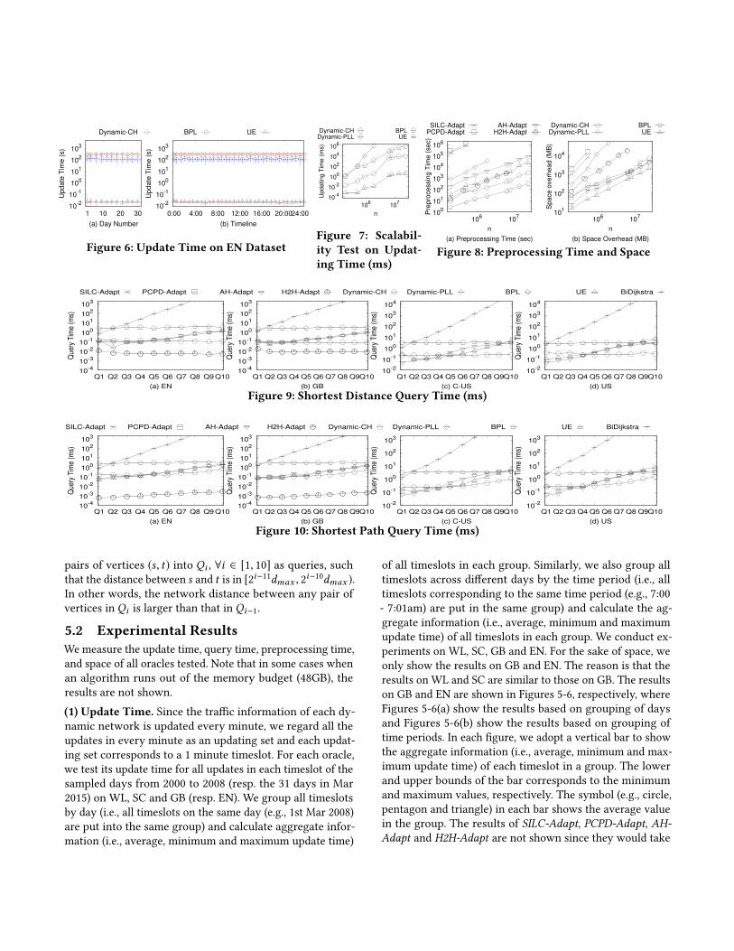
(1) Update Time. Since the traffic information of each dy-
namic network is updated every minute, we regard all the
updates in every minute as an updating set and each updat-
ing set corresponds to a 1 minute timeslot. For each oracle,
we test its update time for all updates in each timeslot of the
sampled days from 2000 to 2008 (resp. the 31 days in Mar
2015) on WL, SC and GB (resp. EN). We group all timeslots
by day (i.e., all timeslots on the same day (e.g., 1st Mar 2008)
are put into the same group) and calculate aggregate infor-
mation (i.e., average, minimum and maximum update time)
of all timeslots in each group. Similarly, we also group all
timeslots across different days by the time period (i.e., all
timeslots corresponding to the same time period (e.g., 7:00
- 7:01am) are put in the same group) and calculate the ag-
gregate information (i.e., average, minimum and maximum
update time) of all timeslots in each group. We conduct ex-
periments on WL, SC, GB and EN. For the sake of space, we
only show the results on GB and EN. The reason is that the
results on WL and SC are similar to those on GB. The results
on GB and EN are shown in Figures 5-6, respectively, where
Figures 5-6(a) show the results based on grouping of days
and Figures 5-6(b) show the results based on grouping of
time periods. In each figure, we adopt a vertical bar to show
the aggregate information (i.e., average, minimum and max-
imum update time) of each timeslot in a group. The lower
and upper bounds of the bar corresponds to the minimum
and maximum values, respectively. The symbol (e.g., circle,
pentagon and triangle) in each bar shows the average value
in the group. The results of SILC-Adapt, PCPD-Adapt, AH-Adapt and H2H-Adapt are not shown since they would take

more than 1 week to finish updating for a single timeslot.
The results of Dynamic-PLL are not shown since it would
run out of our memory budget.
According to these results, UE could be updated in a ne-
glectable amount of time. The update time of Dynamic-CH,Dynamic-PLL and BPL is several orders of magnitude larger
than ours on WL and SC. Besides, on GB and EN, the update
time of BPLand CH both exceeds 1 minute for most updating
sets, which means they could not meet the hard require-
ment of the updating in practice. On GB, the update time
of each oracle fluctuates from day to day (Figure 5(a)) but
keeps almost steady in different time periods (Figure 5(b)).
The reason is that the number of edges to be updated in each
updating set (corresponding to 1min timeslot) varies a lot
in different days but keeps almost intact in different time
periods. On EN, the update time of each oracle keeps almost
steady (Figure 6(a) and (b)) since on EN, the number of edges
to be updated in each updating set (corresponding to 1min
timeslot) does not vary too much in all timeslots.
We also do a scalability test on the update time based on
all the eight datasets including those with synthetic update
data so that datasets with different sizes (denoted by n) areused. The results are presented in Figure 7. According to
this figure, our UE oracle is scalable and outperforms the
baselines by several orders of magnitude.
Although only our UE oracle could handle the update
operation efficiently (i.e., the data update time is within the
processing time for update), in the following, for the sake
of interest, we also compare UE with other existing oracles
described before in other measurements (i.e., query time,
preprocessing time and space).
(2) Query Time. Figure 9 (resp. Figure 10) presents the
shortest distance (resp. path) query time of the tested oracles.
For the sake of the limited space, we only show the results
on the 4 largest datasets as shown in Table 2. As these results
generally show, (1) for queries with relatively smaller short-
est distances (e.g., Q1-5), all algorithms except for BiDijkstraand BPL perform quite well and have comparable query time;
(2) for other queries (e.g., Q6-10), H2H-Adapt works the bestin most cases (note that H2H-Adapt takes more than one
week to finish updating a single time slot in our previous
experiment); and (3) our UE oracle works fairly well for all
queries on all datasets (e.g., the query time is at most 10ms).
(3) Preprocessing Time and Space. Figures 8(a) and (b)
show the preprocessing time and the space of the tested ora-
cles on the networks (with varying sizes). As shown in Fig-
ure 8(a), (1) PCPD-Adapt and SILC-Adapt have their prepro-cessing time multiple orders of magnitude larger than that of
other oracles and thus cannot scale up to large or even mod-
erate size datasets; (2) Dynamic-PLL and H2H-Adapt have asmaller preprocessing time compared with PCPD-Adapt and
SILC-Adapt but still cannot scale up to large datasets; and (3)
our UE oracle has its preprocessing time the third smallest
and can scale up to the largest dataset in our experiments. As
shown in Figure 8(b), PCPD-Adapt, SILC-Adapt, andDynamic-PLL have their space 1-3 orders of magnitude larger than
that of other algorithms and cannot scale up to large datasets
and all other oracles have their space comparable but our UEoracle has clearly the smallest space.
(4) Experimental Summary. Firstly, our UE oracle is su-
perior over all existing ones for applications, where it is
required that update needs to be handled in time (simply
because our UE can handle the updates very quickly while
none of the existing oracles can handle the update before the
next batch of update arrives). Secondly, our UE oracle allows
for very efficient query processing (e.g., less than 10ms for
all queries on all datasets tested in this paper), needs quite
affordable processing time (e.g., a few hours for the largest
dataset), and costs the smallest space. Thirdly, PCPD-Adapt,SILC-Adapt, Dynamic-PLL and H2H-Adapt have serious prob-lem on their space that are 2-3 orders of magnitude larger
than others and could not scale up to sizable datasets. Be-
sides, each baseline has an update time more than 2 orders
of magnitude larger than that of UE.
6 CONCLUSIONThe paper studies the shortest distance and path queries
on the dynamic road network and develops a very efficient
oracle for this problem. This oracle has decent theoretical
bounds on the preprocessing time, space, query time and
update time. Remarkably, it enjoys anO(n log2 n) preprocess-ing time and an O(log3 n) update time w.h.p.. However, the
existing oracles all have a worse-than O(n1.5) preprocessingtime and a worse-thanO(n1.5) update time, which shows that
they are not scalable. Our extensive empirical study verifies
that the existing oracles sustain the short updating time in
practice. Besides, our oracle significantly outperforms the
existing works in terms of the update time. The query time,
preprocessing time and space of our oracle is comparable
with the best existing work.
Acknowledgements: We are grateful to the anonymous
reviewers for their constructive comments on this paper.
The research of Victor Junqiu Wei and Raymond Chi-Wing
Wong is supported by HKRGC GRF 16214017. The research
of Cheng Long is supported by the Nanyang Technological
University Start-UP Grant from the College of Engineering
under Grant M4082302 and by the Ministry of Education, Sin-
gapore, under its Academic Research Fund Tier 1 (RG20/19
(S)).
REFERENCES[1] http://download.geofabrik.de.
[2] http://mathworld.wolfram.com/treewidth.html.
[3] https://data.cityofnewyork.us/transportation/real-time-traffic-speed-
data/xsat-x5sa.
[4] https://data.gov.uk/dataset/dft-eng-srn-routes-journey-
times/resource/34b91717-ccfa-46bd-b6f1-a51c4aeacea9.
[5] Fire services department, hong kong: Performance pledge. In
http://www.hkfsd.gov.hk/eng/performance.html, 2020.[6] Virginia department of transportation. In
https://www.virginiadot.org/projects/faq-road-built.asp, 2020.[7] I. Abraham, D. Delling, A. V. Goldberg, and R. F. Werneck. Hierarchical
hub labelings for shortest paths. In Algorithms–ESA 2012. 2012.[8] I. Abraham, A. Fiat, A. V. Goldberg, and R. F. Werneck. Highway
dimension, shortest paths, and provably efficient algorithms. In SODA,2010.
[9] T. Akiba, Y. Iwata, K.-i. Kawarabayashi, and Y. Kawata. Fast shortest-
path distance queries on road networks by pruned highway labeling.
In ALENEX, 2014.[10] T. Akiba, Y. Iwata, and Y. Yoshida. Fast exact shortest-path distance
queries on large networks by pruned landmark labeling. In SIGMOD,2013.
[11] T. Akiba, Y. Iwata, and Y. Yoshida. Dynamic and historical shortest-
path distance queries on large evolving networks by pruned landmark
labeling. In WWW, 2014.
[12] M. Barthélemy. Spatial networks. Physics Reports, 2011.[13] H. Bast, S. Funke, and D. Matijević. Transit: ultrafast shortest-path
queries with linear-time preprocessing. In 9th DIMACS ImplementationChallenge—Shortest Path, 2006.
[14] H. Bast, S. Funke, P. Sanders, and D. Schultes. Fast routing in road
networks with transit nodes. Science, 2007.[15] G. V. Batz, D. Delling, P. Sanders, and C. Vetter. Time-dependent
contraction hierarchies. In Proceedings of the Meeting on AlgorithmEngineering & Expermiments, 2009.
[16] L. Benguigui. A fractal analysis of the public transportation system of
paris. Environment and Planning A, 1995.[17] L. Benguigui and M. Daoud. Is the suburban railway system a fractal?
Geographical Analysis, 1991.[18] A. Bernstein and D. Karger. Improved distance sensitivity oracles via
random sampling. In SODA, 2008.[19] A. Bernstein and D. Karger. A nearly optimal oracle for avoiding failed
vertices and edges. In STOC, 2009.[20] A. Beygelzimer, S. Kakade, and J. Langford. Cover trees for nearest
neighbor. In ICML, 2006.[21] E. Cohen, E. Halperin, H. Kaplan, and U. Zwick. Reachability and
distance queries via 2-hop labels. SIAM Journal on Computing, 2003.[22] G. Csányi and B. Szendrői. Fractal–small-world dichotomy in real-
world networks. Physical Review E, 2004.[23] L. Daqing, K. Kosmidis, A. Bunde, and S. Havlin. Dimension of spatially
embedded networks. Nature Physics, 2011.[24] U. Demiryurek, F. Banaei-Kashani, C. Shahabi, and A. Ranganathan.
Online computation of fastest path in time-dependent spatial networks.
In SSTD, 2011.[25] U. Demiryurek, B. Pan, F. Banaei-Kashani, and C. Shahabi. Towards
modeling the traffic data on road networks. In Proceedings of the SecondInternational Workshop on Computational Transportation Science, 2009.
[26] J. Dibbelt, B. Strasser, and D. Wagner. Customizable contraction hier-
archies. Journal of Experimental Algorithmics (JEA), 2016.[27] E. W. Dijkstra. A note on two problems in connexion with graphs.
Numerische mathematik, 1959.
[28] J. Gao, Q. Zhao, W. Ren, A. Swami, R. Ramanathan, and A. Bar-Noy.
Dynamic shortest path algorithms for hypergraphs. IEEE/ACM Trans-actions on networking, 2014.
[29] R. Geisberger, P. Sanders, D. Schultes, and D. Delling. Contraction
hierarchies: Faster and simpler hierarchical routing in road networks.
In Experimental Algorithms. 2008.[30] R. Geisberger, P. Sanders, D. Schultes, and C. Vetter. Exact routing
in large road networks using contraction hierarchies. TransportationScience, 2012.
[31] A. V. Goldberg and C. Harrelson. Computing the shortest path: A
search meets graph theory. In SODA, 2005.[32] L. Guo, Y. Zhu, Z. Luo, andW. Li. The scaling of several public transport
networks in china. Fractals, 2013.[33] R. H. Güting. An introduction to spatial database systems. VLDBJ,
1994.
[34] T. Hayashi, T. Akiba, and K.-i. Kawarabayashi. Fully dynamic shortest-
path distance query acceleration on massive networks. In CIKM, 2016.
[35] G. B. Hermsdorff and L. Gunderson. A unifying framework for
spectrum-preserving graph sparsification and coarsening. In Advancesin Neural Information Processing Systems, 2019.
[36] R. Jin, N. Ruan, Y. Xiang, and V. Lee. A highway-centric labeling
approach for answering distance queries on large sparse graphs. In
SIGMOD, 2012.[37] S. Jung and S. Pramanik. Hiti graph model of topographical road maps
in navigation systems. In ICDE, 1996.[38] S. Jung and S. Pramanik. An efficient path computation model for
hierarchically structured topographical road maps. TKDE, 2002.[39] E. Kanoulas, Y. Du, T. Xia, and D. Zhang. Finding fastest paths on a
road network with speed patterns. In ICDE, 2006.[40] D. R. Karger and M. Ruhl. Finding nearest neighbors in growth-
restricted metrics. In STOC, 2002.[41] D. Knuth. Seminumerical algorithms, the art of computer program-
ming, vol. 2 addison-wesley. Reading, MA, 1997.[42] R. Lambiotte, V. D. Blondel, C. De Kerchove, E. Huens, C. Prieur,
Z. Smoreda, and P. Van Dooren. Geographical dispersal of mobile
communication networks. Physica A: Statistical Mechanics and itsApplications, 2008.
[43] S. Lämmer, B. Gehlsen, and D. Helbing. Scaling laws in the spatial
structure of urban road networks. Physica A: Statistical Mechanics andits Applications, 2006.
[44] J.-R. Lee and C.-W. Chung. Efficient distance sensitivity oracles for
real-world graph data. TKDE, 2019.[45] L. Li, S. Wang, and X. Zhou. Time-dependent hop labeling on road
network. In ICDE, 2019.[46] D. Ouyang, L. Qin, L. Chang, X. Lin, Y. Zhang, and Q. Zhu. When
hierarchy meets 2-hop-labeling: Efficient shortest distance queries on
road networks. In SIGMOD, 2018.[47] D. Papadias, J. Zhang, N. Mamoulis, and Y. Tao. Query processing in
spatial network databases. In VLDB, 2003.[48] Y. Qin, Q. Z. Sheng, and W. E. Zhang. Sief: Efficiently answering
distance queries for failure prone graphs. In EDBT, 2015.[49] A. K. Rai and S. Agarwal. Maintaining shortest path tree in dynamic
digraphs having negative edge-weights. In International Conferenceon Parallel Distributed Computing Technologies and Applications, 2011.
[50] H. Samet, J. Sankaranarayanan, and H. Alborzi. Scalable network
distance browsing in spatial databases. In SIGMOD, 2008.[51] P. Sanders and D. Schultes. Highway hierarchies hasten exact shortest
path queries. In European Symposium on Algorithms (ESA). 2005.[52] P. Sanders and D. Schultes. Engineering highway hierarchies. In
European Symposium on Algorithms (ESA). 2006.[53] J. Sankaranarayanan and H. Samet. Distance oracles for spatial net-
works. In ICDE, 2009.

[54] J. Sankaranarayanan and H. Samet. Query processing using distance
oracles for spatial networks. TKDE, 2010.[55] J. Sankaranarayanan, H. Samet, and H. Alborzi. Path oracles for spatial
networks. VLDB, 2009.[56] D. Schultes and P. Sanders. Dynamic highway-node routing. In
Experimental Algorithms. 2007.[57] S. Wang, W. Lin, Y. Yang, X. Xiao, and S. Zhou. Efficient route planning
on public transportation networks: A labelling approach. In SIGMOD,2015.
[58] Y. Wang, G. Li, and N. Tang. Querying shortest paths on time depen-
dent road networks. VLDB, 2019.[59] V. J. Wei, R. C.-W. Wong, and C. Long. Fastest path and time queries on
dynamic spatial networkswith poly-logarithmic update time (technical
report). In http://home.cse.ust.hk/~raywong/paper/sigmod20-dynamic-technical.pdf.
[60] O. Weimann and R. Yuster. Replacement paths and distance sensitivity
oracles via fast matrix multiplication. ACM Transactions on Algorithms(TALG), 2013.
[61] L. Wu, X. Xiao, D. Deng, G. Cong, A. D. Zhu, and S. Zhou. Shortest path
and distance queries on road networks: An experimental evaluation.
VLDB, 2012.[62] Y. Yuan, X. Lian, G. Wang, Y. Ma, and Y. Wang. Constrained shortest
path query in a large time-dependent graph. VLDB, 2019.[63] A. D. Zhu, H. Ma, X. Xiao, S. Luo, Y. Tang, and S. Zhou. Shortest path
and distance queries on road networks: towards bridging theory and
practice. In SIGMOD, 2013.
Recommended