Applied Statistics and Probability for Engineers
Copyright © 2014 John Wiley & Sons, Inc. All rights reserved.Copyright © 2014 John Wiley & Sons, Inc. All rights reserved.
Chapter 10Statistical Inference for Two Samples
Sixth Edition
Douglas C. Montgomery George C. Runger

10 Statistical Inference for Two Samples
10-1 Inference on the Difference in Means of
Two Normal Distributions, Variances Known
10-1.1 Hypothesis tests on the difference in means,
variances known10-1.2 Type II error and choice of sample size10-1.3 Confidence interval on the difference in
means, variance known
10-2 Inference on the Difference in Means of
10-5.2 Hypothesis tests on the ratio of two variances
10-5.3 Type II error and choice of sample size
10-5.4 Confidence interval on the ratio of two variances
10-6 Inference on Two Population
CHAPTER OUTLINE
Copyright © 2014 John Wiley & Sons, Inc. All rights reserved.
2
10-2 Inference on the Difference in Means of
Two Normal Distributions, Variance Unknown10-2.1 Hypothesis tests on the difference in means,
variances unknown10-2.2 Type II error and choice of sample size10-2.3 Confidence interval on the difference in
means, variance unknown
10-3 A Nonparametric Test on the Difference
in Two Means
10-4 Paired t-Tests
10-5 Inference on the Variances of Two
Normal Populations
10-5.1 F distributions
10-6 Inference on Two Population
Proportions
10-6.1 Large sample tests on the
difference in population proportions
10-6.2 Type II error and choice of sample size
10-6.3 Confidence interval on the difference in population proportions
10-7 Summary Table and
Roadmap for Inference
Procedures for Two Samples
Chapter 10 Title and Outline
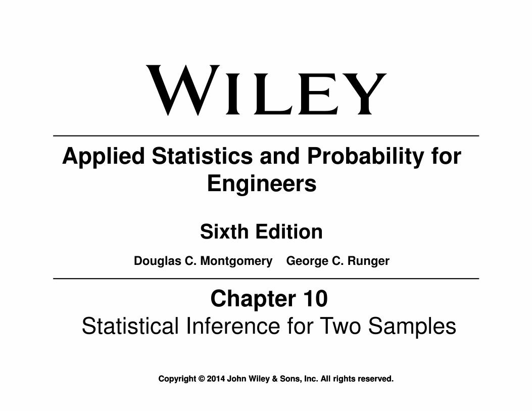
Case1: Inference on the Difference in Means of Two Normal Distributions, Variances Known
Assumptions1. Let be a random sample from population 1.
2. Let be a random sample from population 2.
3. The two populations X1 and X2 are independent.
4. Both X and X are normal.
111211 ,,, nXXX K
222221 ,,, nXXX K
Copyright © 2014 John Wiley & Sons, Inc. All rights reserved.
3
4. Both X1 and X2 are normal.
Sec 10-1 Inference on the Difference in Means of Two Normal Distributions, Variances Known

Null hypothesis: H0: µ1 − µ2 = ∆0
Test statistic: (10-2)
2
22
1
21
0210
nn
XXZ
σ+
σ
∆−−=
Alternative Hypotheses P-Value Rejection Criterion For Fixed-Level Tests
Case1: Inference on the Difference in Means of Two Normal Distributions, Variances Known
Copyright © 2014 John Wiley & Sons, Inc. All rights reserved.
4
Fixed-Level Tests
H0: µ1 − µ2 ≠ ∆0 Probability above |z0| and probability below − |z0|, P
= 2[1 − Φ(|z0|)]
|z0|> zα/2
H1: µ1 − µ2 > ∆0 Probability above z0, P = 1 − Φ(z0)
z0 > zα
H1: µ1 − µ2 < ∆0 Probability below z0, P = Φ(z0)
z0 < −zα
Sec 10-1 Inference on the Difference in Means of Two Normal Distributions, Variances Known
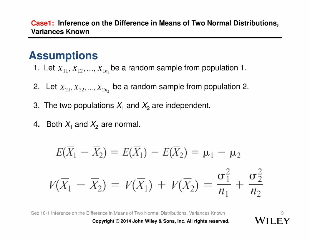
EXAMPLE 10-1 Paint Drying Time
A product developer is interested in reducing the drying time of a primer paint. Two formulations of the paint are tested; formulation 1 is the standard chemistry, and formulation 2 has a new drying ingredient that should reduce the drying time. From experience, it is known that the standard deviation of drying time is 8 minutes, and this inherent variability should be unaffected by the addition of the new ingredient. Ten specimens are painted with formulation 1, and another 10 specimens are painted with formulation 2; the 20 specimens are painted in random order. The two sample average drying times are minutes and minutes, respectively. What conclusions can the product developer draw about the effectiveness of the new ingredient, using α = 0.05?
1211 =x 1122 =x
Copyright © 2014 John Wiley & Sons, Inc. All rights reserved.
5
ingredient, using α = 0.05?
The eight-step procedure is:
1. Parameter of interest: The difference in mean drying times, µ1 − µ2, and ∆0 = 0.
2. Null hypothesis: H0: µ1 − µ2 = 0.
3. Alternative hypothesis: H1: µ1 > µ2.4. α = 0.05
Sec 10-1 Inference on the Difference in Means of Two Normal Distributions, Variances Known
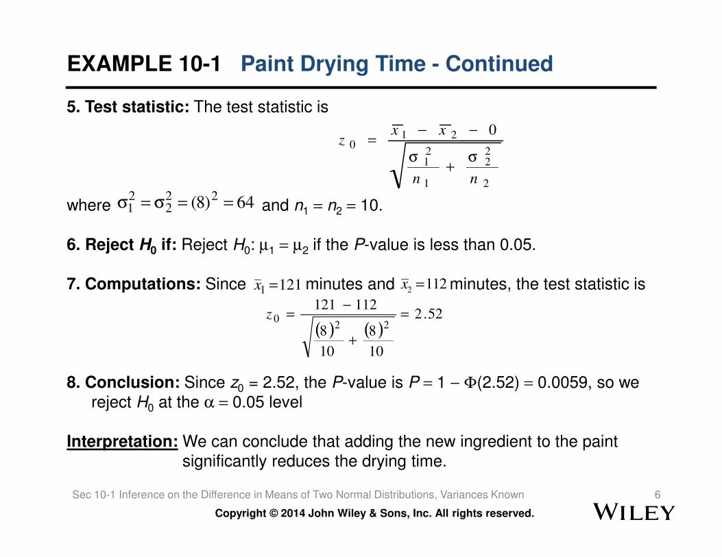
EXAMPLE 10-1 Paint Drying Time - Continued
5. Test statistic: The test statistic is
where and n1 = n2 = 10.
6. Reject H0 if: Reject H0: µ1 = µ2 if the P-value is less than 0.05.
7. Computations: Since minutes and minutes, the test statistic is
2
22
1
21
210
0
nn
xxz
σ+
σ
−−=
64)8(22
221 ==σ=σ
121=x 112x =
Copyright © 2014 John Wiley & Sons, Inc. All rights reserved.
6
7. Computations: Since minutes and minutes, the test statistic is
8. Conclusion: Since z0 = 2.52, the P-value is P = 1 − Φ(2.52) = 0.0059, so we reject H0 at the α = 0.05 level
Interpretation: We can conclude that adding the new ingredient to the paint significantly reduces the drying time.
1211 =x 2112x =
( ) ( )52.2
10
8
10
8
112121
220 =
+
−=z
Sec 10-1 Inference on the Difference in Means of Two Normal Distributions, Variances Known

Case 1: Confidence Interval on a Difference in Means, Variances Known
If and are the means of independent random samples of sizes n1 and n2 from two independent normal populations with known variance and , respectively, a 100(1 −α−α−α−α)%%%%confidence interval for µµµµ1 −−−− µµµµ2 is
1x2
x
21σ
2
2σ
22
21
22
21 zxxzxx
σ+
σ+−≤µ−µ≤
σ+
σ−− (10-7)
Copyright © 2014 John Wiley & Sons, Inc. All rights reserved.
7
where zα/2 is the upper α/2 percentage point of the standard normal distribution
2
2
1
12/2121
2
2
1
1/221
nnzxx
nnzxx
σ+
σ+−≤µ−µ≤
σ+
σ−− αα (10-7)
Sec 10-1 Inference on the Difference in Means of Two Normal Distributions, Variances Known

EXAMPLE 10-4 Aluminum Tensile Strength
Tensile strength tests were performed on two different grades of aluminum spars used in manufacturing the wing of a commercial transport aircraft. From past experience with the spar manufacturing process and the testing procedure, the standard deviations of tensile strengths are assumed to be known. The data obtained are as follows: n1 = 10, , σ1 = 1, n2 = 12, , and σ2 = 1.5. If µ1 and µ2 denote the true mean tensile strengths for the two grades of spars, we may find a 90% confidence interval on the difference in mean strength µ1 − µ2
as follows:
6.871 =x 274.5x =
21
22
21
/221 µ−µ≤σ
+σ
−− αnn
zxx
Copyright © 2014 John Wiley & Sons, Inc. All rights reserved.
8
12
)5.1(
10
)1(645.15.746.87
12
)5.1(
10
)1(645.15.746.87
22
21
22
2
22
1
21
2/21
2121
/221
++−≤
µ−µ≤+−−
σ+
σ+−≤
µ−µ≤+−−
α
α
nnzxx
nnzxx
98.1322.12 21 ≤−≤ µµ
Sec 10-1 Inference on the Difference in Means of Two Normal Distributions, Variances Known

One-Sided Confidence Bounds
Upper Confidence Bound
2
22
1
21
2121nn
zxxσ
+σ
+−≤µ−µ α(10-9)
Case 1: Confidence Interval on a Difference in Means, Variances Known
Copyright © 2014 John Wiley & Sons, Inc. All rights reserved.
Lower Confidence Bound
9
21
212
22
1
21
21 µ−µ≤σ
+σ
−− αnn
zxx (10-10)
Sec 10-1 Inference on the Difference in Means of Two Normal Distributions, Variances Known
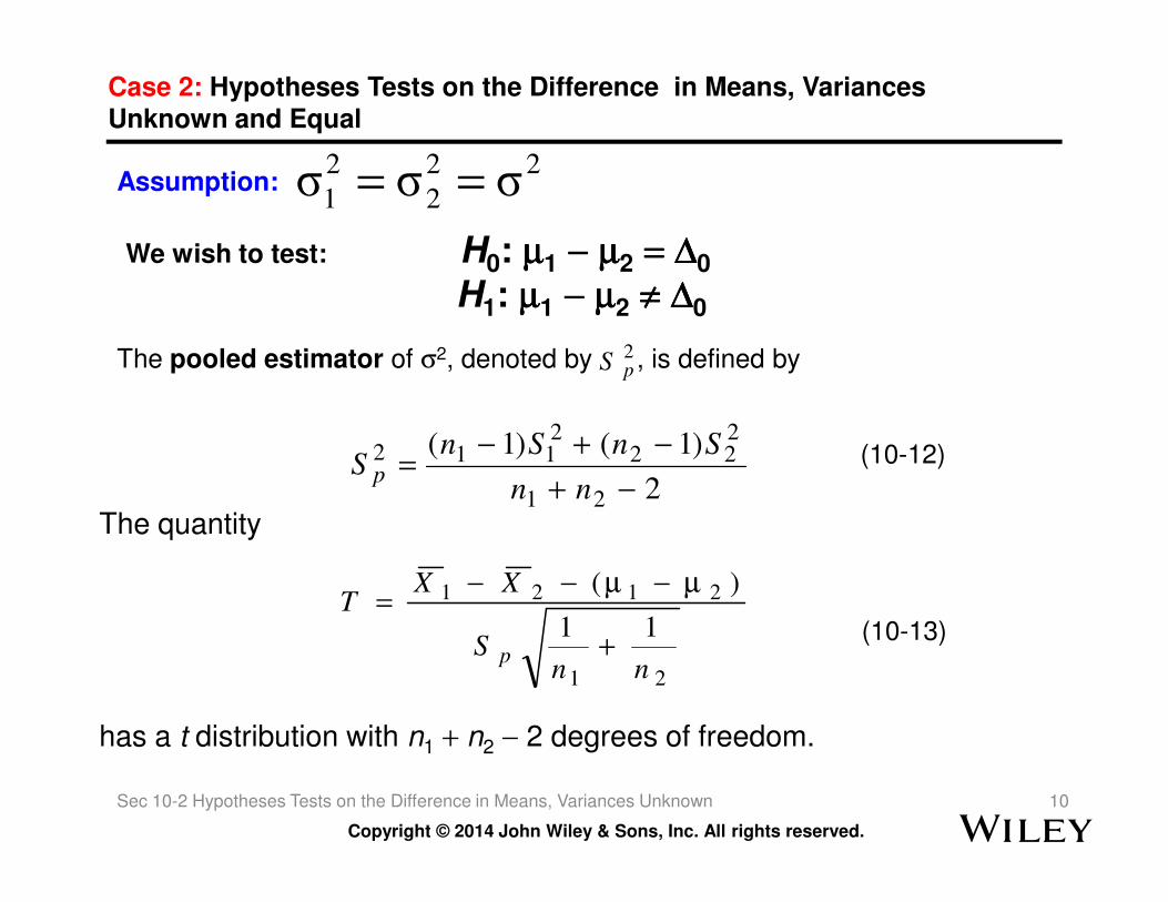
Case 2: Hypotheses Tests on the Difference in Means, Variances Unknown and Equal
We wish to test: H0: µµµµ1 −−−− µµµµ2 ==== ∆∆∆∆0
H1: µµµµ1 −−−− µµµµ2 ≠≠≠≠ ∆∆∆∆0
Assumption:22
2
2
1 σσσ ==
The pooled estimator of σ2, denoted by , is defined by
(10-12)
2pS
)1()1(222
2112 −+−
=SnSn
S
Copyright © 2014 John Wiley & Sons, Inc. All rights reserved.
10
(10-12)
2
)1()1(
21
22112
−+
−+−=
nn
SnSnS p
The quantity
(10-13)
has a t distribution with n1 + n2 − 2 degrees of freedom.
21
2121
11
)(
nnS
XXT
p +
µ−µ−−=
Sec 10-2 Hypotheses Tests on the Difference in Means, Variances Unknown

Case 2: Tests on the Difference in Means of Two Normal Distributions, Variances Unknown and Equal
Null hypothesis: H0: µ1 − µ2 = ∆0
Test statistic: (10-14)
Alternative Hypothesis P-Value
Rejection Criterion for Fixed-Level Tests
µ − µ ≠ ∆ | |
21
0210
11
nnS
XXT
p +
∆−−=
Copyright © 2014 John Wiley & Sons, Inc. All rights reserved.
11
H1: µ1 − µ2 ≠ ∆0 Probability above |t0| and probability below−|t0|
or
H1: µ1 − µ2 > ∆0 Probability above t0H1: µ1 − µ2 < ∆0 Probability below t0
2,2/0 21 −+α> nntt
2,2/0 21 −+α−< nntt
2,0 21 −+α> nntt
2,0 21 −+α−< nntt
Sec 10-2 Hypotheses Tests on the Difference in Means, Variances Unknown

EXAMPLE 10-5 Yield from a Catalyst
Two catalysts are being analyzed to determine how they affect the mean yield of a chemical process. Specifically, catalyst 1 is currently in use, but catalyst 2 is acceptable. Since catalyst 2 is cheaper, it should be adopted, providing it does not change the process yield. A test is run in the pilot plant and results in the data shown in Table 10-1. Is there any difference between the mean yields? Use α = 0.05, and assume equal variances.
Observation Number Catalyst 1 Catalyst 2
1 91.50 89.19
Copyright © 2014 John Wiley & Sons, Inc. All rights reserved.
12
1 91.50 89.19
2 94.18 90.95
3 92.18 90.46
4 95.39 93.21
5 91.79 97.19
6 89.07 97.04
7 94.72 91.07
8 89.21 92.75
s1 = 2.39 s2 = 2.98
255.921 =x 733.922 =x
Sec 10-2 Hypotheses Tests on the Difference in Means, Variances Unknown

EXAMPLE 10-5 Yield from a Catalyst - Continued
The eight-step hypothesis-testing procedure is as follows:
1. Parameter of interest: The parameters of interest are µ1 and µ2, the mean process yield using catalysts 1 and 2, respectively.
2. Null hypothesis: H0: µ1 = µ2
3. Alternative hypothesis: H1: µ1 ≠ µ2
Copyright © 2014 John Wiley & Sons, Inc. All rights reserved.
13
3. Alternative hypothesis: H1: µ1 ≠ µ2
4. α = 0.05
5. Test statistic: The test statistic is
6. Reject H0 if: Reject H0 if the P-value is less than 0.05.
21
210
11
0
nns
xxt
p +
−−=
Sec 10-2 Hypotheses Tests on the Difference in Means, Variances Unknown

EXAMPLE 10-5 Yield from a Catalyst - Continued
7. Computations: From Table 10-1 we have , s1 = 2.39, n1 = 8, , s2 = 2.98, and n2 = 8.
Therefore
and
255.921 =x
292.733x =
70.230.7
30.7288
)98.2(7)39.2()7(
2
)1()1( 22
21
222
2112
==
=−+
+=
−+
−+−=
p
p
s
nn
snsns
35.011
733.92255.92
11
210 −=
−=
−=
xxt
Copyright © 2014 John Wiley & Sons, Inc. All rights reserved.
14
8. Conclusions: From Appendix Table V we can find t0.40,14 = 0.258 and t0.25,14 = 0.692. Since, 0.258 < 0.35 < 0.692, we conclude that lower and upper bounds on the P-value are 0.50 < P < 0.80. Therefore, since the P-value exceeds α = 0.05, the null hypothesis cannot be rejected.Interpretation: At 5% level of significance, we do not have strong evidence to conclude that catalyst 2 results in a mean yield that differs from the mean yield when catalyst 1 is used.
35.0
8
1
8
170.2
1170.2
21
0 −=
+
=
+
=
nn
t
Sec 10-2 Hypotheses Tests on the Difference in Means, Variances Unknown

Case2: Confidence Interval on the Difference in Means, Variance Unknown
Assumption: 22
2
2
1 σ=σ=σIf , and are the sample means and variances of two random samples of sizes n1 and n2, respectively, from two independent normal populations with unknown but equal variances, then a 100(1 - α)% confidence interval on the difference in means µ1 - µ2 is
2121 ,, sxx 2
2s
212/2,21
1121 nn
stxx pnn +−− −+α
Copyright © 2014 John Wiley & Sons, Inc. All rights reserved.
15
(10-19)
where is the pooled estimate of the common population standard deviation, and is the upper α/2 percentage point of the t distribution with n1 + n2 - 2 degrees of freedom.
212/2,2121
21
11
21 nnstxx
nn
pnn ++−≤µ−µ≤ −+α
)2]/()1()1[( 21222
211 −+−+−= nnsnsns p
2/2, 21 −+α nnt
Sec 10-2 Hypotheses Tests on the Difference in Means, Variances Unknown

Example 10-9 Cement Hydration
Ten samples of standard cement had an average weight percent calcium of
with a sample standard deviation of s1 = 5.0, and 15 samples of the lead-doped cement
had an average weight percent calcium of with a sample standard deviation of
s2 = 4.0. Assume that weight percent calcium is normally distributed with same standard
deviation. Find a 95% confidence interval on the difference in means, µ1 - µ2, for the two
types of cement.
0.901 =x
0.872 =x
The pooled estimate of the common standard deviation is found as follows:
52.1921510
)0.4(14)0.5(9
2
)1()1( 22
21
222
2112 =
−+
+=
−+
−+−=
nn
snsnsp
Copyright © 2014 John Wiley & Sons, Inc. All rights reserved.
16
The 95% confidence interval is found using Equation 10-19:
Upon substituting the sample values and using t0.025,23 = 2.069,
which reduces to -0.72 ≤ µ1 - µ2 ≤ 6.72
21510221 −+−+ nn
4.452.19 ==ps
2123,025.02121
2123,025.021
1111
nnstxx
nnstxx pp ++−≤µ−µ≤+−−
( ) ( )15
1
10
14.4069.20.870.90
15
1
10
14.4069.20.870.90 21 ++−≤µ−µ≤+−−
Sec 10-2 Hypotheses Tests on the Difference in Means, Variances Unknown

2
2
2
1σ≠σAssumption:
2
22
1
21
021*0
n
S
n
S
XXT
+
∆−−=
If H0: µ1 − µ2 = ∆0 is true, the statistic
Case3: Hypotheses Tests on the Difference in Means, Variances Unknown and Unequal
(10-15)
Copyright © 2014 John Wiley & Sons, Inc. All rights reserved.
17
is distributed as t with degrees of freedom given by
(10-16)( ) ( )
1
/
1
/
2
2
222
1
2
12
1
2
2
22
1
21
−+
−
+
=
n
ns
n
ns
n
s
n
s
v
Sec 10-2 Hypotheses Tests on the Difference in Means, Variances Unknown

EXAMPLE 10-6 Arsenic in Drinking Water
Arsenic concentration in public drinking water supplies is a potential health risk. An article in the Arizona Republic (May 27, 2001) reported drinking water arsenic concentrations in parts per billion (ppb) for 10 metropolitan Phoenix communities and 10 communities in rural Arizona. The data follow:
Metro Phoenix Rural Arizona( , s1 = 7.63) ( , s2 = 15.3)Phoenix, 3 Rimrock, 48Chandler, 7 Goodyear, 44Gilbert, 25 New River, 40Glendale, 10 Apache Junction, 38
12.51 ====x 27.52 ====x
Copyright © 2014 John Wiley & Sons, Inc. All rights reserved.
18
Determine if there is any difference in mean arsenic concentrations between metropolitan Phoenix communities and communities in rural Arizona.
Glendale, 10 Apache Junction, 38Mesa, 15 Buckeye, 33Paradise Valley, 6 Nogales, 21Peoria, 12 Black Canyon City, 20Scottsdale, 25 Sedona, 12Tempe, 15 Payson, 1Sun City, 7 Casa Grande, 18
Sec 10-2 Hypotheses Tests on the Difference in Means, Variances Unknown

EXAMPLE 10-6 Arsenic in Drinking Water - Continued
The eight-step procedure is:1. Parameter of interest: The parameters of interest are the mean arsenic
concentrations for the two geographic regions, say, µ1 and µ2, and we are interested in determining whether µ1 − µ2 = 0.
2. Non hypothesis: H0: µ1 − µ2 = 0, or H0: µ1 = µ2
3. Alternative hypothesis: H1: µ1 ≠ µ2
4. α = 0.05
5. Test statistic: 21*
0
0xxt
−−=
Copyright © 2014 John Wiley & Sons, Inc. All rights reserved.
19
5. Test statistic: The test statistic is
6. Reject H0 if : The degrees of freedom on are found as2
22
1
21
0
n
s
n
s
t
+
=
( ) ( )
( ) ( )
( )[ ] ( )[ ]132.13
9
/103.15
9
/1063.7
10
3.15
10
63.7
1
/
1
/
~2222
222
2
2
222
1
2
12
1
2
2
22
1
21
−=
+
+
=
−+
−
+
=
n
ns
n
ns
n
s
n
s
v
Sec 10-2 Hypotheses Tests on the Difference in Means, Variances Unknown

Therefore, using α = 0.05 and a fixed-significance-level test, we would reject H0: µ1 = µ2 if or if .
7. Computations: Using the sample data we find
( ) ( )77.2
3.1563.7
5.275.12
2222
21
21*0 −=
+
−=
+
−=
ss
xxt
160.213,025.0*0 => tt 160.213,025.0
*0 −=−< tt
EXAMPLE 10-6 Arsenic in Drinking Water - Continued
Copyright © 2014 John Wiley & Sons, Inc. All rights reserved.
20
8. Conclusions: Because , we reject the null hypothesis.
Interpretation: We can conclude that mean arsenic concentration in the drinking water in rural Arizona is different from the mean arsenic concentration in metropolitan Phoenix drinking water.
101021
++nn
160.277.2 13,025.0*0 −=<−= tt
Sec 10-2 Hypotheses Tests on the Difference in Means, Variances Unknown

Case3: Confidence Interval on the Difference in Means, Variance Unknown and Unequal
Assumption : 2
2
2
1 σ≠σ
If , and are the means and variances of two random samples of sizes n1 and n2, respectively, from two independent normal populations with unknown and unequal variances, an approximate 100(1 - α)% confidence interval on the difference in means µ1 - µ2 is
2121 ,, sxx 2
2s
2222
Copyright © 2014 John Wiley & Sons, Inc. All rights reserved.
21
(10-20)
where v is given by Equation 10-16 and tα/2,v the upper α /2 percentage point of the
t distribution with v degrees of freedom.
2
22
1
21
,2/21212
22
1
21
/2,21n
s
n
stxx
n
s
n
stxx vv ++−≤µ−µ≤+−− αα
Sec 10-2 Hypotheses Tests on the Difference in Means, Variances Unknown

10-5.1 The F Distribution
Case 5: Inferences on the Variances of Two Normal Populations
We wish to test the hypotheses:
22
211
22
210
:
:
σ≠σ
σ=σ
H
H
Let W and Y be independent chi-square random variables with u and v degrees of freedom respectively. Then the ratio
(10-28)uWF
/=
Copyright © 2014 John Wiley & Sons, Inc. All rights reserved.
22
(10-28)
has the probability density function
(10-29)
and is said to follow the distribution with u degrees of freedom in the numerator and v degrees of freedom in the denominator. It is usually abbreviated as Fu,v.
vY
uWF
/
/=
( ) ∞<<
+
Γ
Γ
+Γ
=+
−
x
xv
uvu
xv
uvu
xfvu
uu
0,
122
2)(
/2
1/2)(/2
Sec 10-5 Inferences on the Variances of Two Normal Populations

Case 5: Hypothesis Tests on the Ratio of Two Variances
Let be a random sample from a normal population with mean µ1 and variance , and let
be a random sample from a second normal population with mean µ 2 and variance . Assume that both normal populations are independent. Let and be the sample variances. Then the ratio
111211 ,,, nXXX K
21σ
222221 ,,, nXXX K
2
2σ
21S
2
2S
Copyright © 2014 John Wiley & Sons, Inc. All rights reserved.
23
has an F distribution with n1 − 1 numerator degrees of freedom and n2 − 1 denominator degrees of freedom.
22
22
21
21
/
/
σ
σ=
S
SF
Sec 10-5 Inferences on the Variances of Two Normal Populations
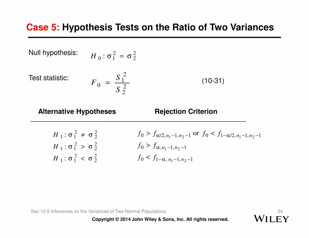
Case 5: Hypothesis Tests on the Ratio of Two Variances
Null hypothesis:
Test statistic:
Alternative Hypotheses Rejection Criterion
22
210 : σ=σH
22
21
0S
SF = (10-31)
Copyright © 2014 John Wiley & Sons, Inc. All rights reserved.
24
22
211
22
211
22
211
:
:
:
σ<σ
σ>σ
σ≠σ
H
H
H
1,1,10
1,1,0
1,1/2,101,1/2,0
21
21
2121or
−−α−
−−α
−−α−−−α
<
>
<>
nn
nn
nnnn
ff
ff
ffff
Sec 10-5 Inferences on the Variances of Two Normal Populations

Example 10-13 Semiconductor Etch Variability
Oxide layers on semiconductor wafers are etched in a mixture of gases to achieve the proper thickness. The variability in the thickness of these oxide layers is a critical characteristic of the wafer, and low variability is desirable for subsequent processing steps. Two different mixtures of gases are being studied to determine whether one is superior in reducing the variability of the oxide thickness. Sixteen wafers are etched in each gas. The sample standard deviations of oxide thickness are s1 = 1.96 angstroms and s2 = 2.13 angstroms, respectively. Is there any evidence to indicate that either gas is preferable? Use a fixed-level test with α = 0.05.
Copyright © 2014 John Wiley & Sons, Inc. All rights reserved.
25
either gas is preferable? Use a fixed-level test with α = 0.05.
The eight-step hypothesis-testing procedure is:
1. Parameter of interest: The parameter of interest are the variances of oxide thickness and .
2. Null hypothesis:
3. Alternative hypothesis:4. α = 0.05
21σ
2
2σ
22
210 : σ=σH
22
211: σ≠σH
Sec 10-5 Inferences on the Variances of Two Normal Populations

Example 10-13 Semiconductor Etch Variability
5. Test statistic: The test statistic is
6. Reject H0 if : Because n1 = n2 = 16 and α = 0.05, we will reject if f0 > f0.025,15,15
= 2.86 or if f0 <f0.975,15,15 = 1/f0.025,15,15 = 1/2.86 = 0.35.
7. Computations: Because and , the test statistic is
22
21
0s
sf =
84.3)96.1(22
1 ==s 54.4)13.2(22
2 ==s
85.084.3
21 ===
sf
Copyright © 2014 John Wiley & Sons, Inc. All rights reserved.
26
8. Conclusions: Because f0..975,15,15 = 0.35 < 0.85 < f0.025,15,15 = 2.86, we cannot reject the null hypothesis at the 0.05 level of significance.
Interpretation: There is no strong evidence to indicate that either gas results in a smaller variance of oxide thickness.
85.054.4
84.322
10 ===
s
sf
22
210 : σ=σH
Sec 10-5 Inferences on the Variances of Two Normal Populations

Case 5: Confidence Interval on the Ratio of Two Variances
If and are the sample variances of random samples of sizes n1 and n2, respectively, from two independent normal populations with unknown variances and , then a 100(1 − α)% confidence interval on the ratio is
(10-33)
21s
2
2s
21σ 2
2σ
2
2
2
1 /σσσσσσσσ
1,1,/222
21
22
21
1,1/2,122
21
1212 −−α−−α− ≤σ
σ≤ nnnn f
s
sf
s
s
Copyright © 2014 John Wiley & Sons, Inc. All rights reserved.
27
where and are the upper and lower α/2 percentage points of the F distribution with n2 – 1 numerator and n1 – 1 denominator degrees of freedom, respectively.
.A confidence interval on the ratio of the standard deviations can be obtained by taking square roots in Equation 10-33.
1,1,/2 12 −−α nnf2 1/2 , 1, 1n n
f1−α − −
Sec 10-5 Inferences on the Variances of Two Normal Populations

Example 10-15 Surface Finish for Titanium Alloy
A company manufactures impellers for use in jet-turbine engines. One of the operations involves grinding a particular surface finish on a titanium alloy component. Two different grinding processes can be used, and both processes can produce parts at identical mean surface roughness. The manufacturing engineer would like to select the process having the least variability in surface roughness. A random sample of n1 = 11 parts from the first process results in a sample standard deviations s1 =5.1 microinches, and a random sample of n = 16 parts from the second process results in a sample standard deviation of
Copyright © 2014 John Wiley & Sons, Inc. All rights reserved.
28
n1 = 16 parts from the second process results in a sample standard deviation of s2 = 4.7 microinches. Find a 90% confidence interval on the ratio of the two standard deviations, σ1 / σ2.
Assuming that the two processes are independent and that surface roughness is normally distributed, we can use Equation 10-33 as follows:
10,15,05.022
21
22
21
10,15,95.022
21 f
s
sf
s
s≤
σ
σ≤
Sec 10-5 Inferences on the Variances of Two Normal Populations

Example 10-15 Surface Finish for Titanium Alloy - Continued
or upon completing the implied calculations and taking square roots,
85.2)7.4(
)1.5(39.0
)7.4(
)1.5(2
2
22
21
2
2
≤σ
σ≤
832.1678.02
1 ≤σ
σ≤
Copyright © 2014 John Wiley & Sons, Inc. All rights reserved.
29
Notice that we have used Equation 10-30 to find
f0.95,15,10 = 1/f0.05,10,15 = 1/2.54= 0.39.
Interpretation: Since this confidence interval includes unity, we cannot claim that the standard deviations of surface roughness for the two processes are different at the 90% level of confidence.
2σ
Sec 10-5 Inferences on the Variances of Two Normal Populations

Case 6:Test on the Difference in Population Proportions
We wish to test the hypotheses:
211
210
:
:
ppH
ppH
≠
=
The following test statistic is distributed approximately
Copyright © 2014 John Wiley & Sons, Inc. All rights reserved.
30
The following test statistic is distributed approximately
as standard normal and is the basis of the test:
(10-34)
2
22
1
11
2121
)1()1(
)(ˆˆ
n
pp
n
pp
ppPPZ
−+
−
−−−=
Sec 10-6 Inference on Two Population Proportions

Case 6: Test on the Difference in Population Proportions
Null hypothesis: H0: p1 = p2
Test statistic:
+−
−=
21
210
11)ˆ1(ˆ
ˆˆ
nnPP
PPZ
Alternative Hypothesis P-ValueRejection Criterion for
Fixed-Level Tests
(10-35)
Copyright © 2014 John Wiley & Sons, Inc. All rights reserved.
31
Alternative Hypothesis P-Value Fixed-Level Tests
H1: p1 ≠ p2 Probability above |z0| and probability below -|z0|. P = 2[1 - Φ(|z0|)]
z0 > zα/2 or z0 < -zα/2
H1: p1 > p2 Probability above z0. P = 1 - Φ(z0)
z0 > zα
H1: p1 < p2 Probability below z0. P = Φ(z0)
z0 < -zα
Sec 10-6 Inference on Two Population Proportions
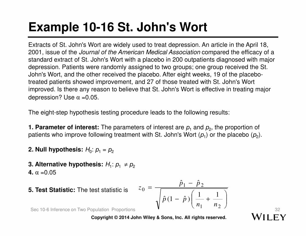
Example 10-16 St. John's Wort
Extracts of St. John's Wort are widely used to treat depression. An article in the April 18,
2001, issue of the Journal of the American Medical Association compared the efficacy of a
standard extract of St. John's Wort with a placebo in 200 outpatients diagnosed with major
depression. Patients were randomly assigned to two groups; one group received the St.
John's Wort, and the other received the placebo. After eight weeks, 19 of the placebo-
treated patients showed improvement, and 27 of those treated with St. John's Wort
improved. Is there any reason to believe that St. John's Wort is effective in treating major
depression? Use α =0.05.
The eight-step hypothesis testing procedure leads to the following results:
Copyright © 2014 John Wiley & Sons, Inc. All rights reserved.
32
1. Parameter of interest: The parameters of interest are p1 and p2, the proportion of
patients who improve following treatment with St. John's Wort (p1) or the placebo (p2).
2. Null hypothesis: H0: p1 = p2
3. Alternative hypothesis: H1: p1 ≠ p2
4. α =0.05
5. Test Statistic: The test statistic is
+−
−=
21
210
11)ˆ1(ˆ
ˆˆ
nnpp
ppz
Sec 10-6 Inference on Two Population Proportions

Example 10-16 St. John's Wort - Continued
where , , n1 = n2 = 100, and
6. Reject H0 if: Reject H0: p1 = p2 if the P-value is less than 0.05.
7. Computations: The value of the test statistic is
27.0/10027ˆ1 ==p 19.0/10019ˆ2 ==p
23.0100100
2719ˆ
21
21 =+
+=
+
+=
nn
xxp
19.027.0 −
Copyright © 2014 John Wiley & Sons, Inc. All rights reserved.
33
8. Conclusions: Since z0 = 1.34, the P-value is P = 2[1 − Φ(1.34)] = 0.18, we cannot reject the null hypothesis.
Interpretation: There is insufficient evidence to support the claim that St. John's Wort is effective in treating major depression.
34.1
100
1
100
1)77.0(23.0
19.027.00 =
+
−=z
Sec 10-6 Inference on Two Population Proportions

Case 6: Confidence Interval on the Difference in the Population Proportions
If and are the sample proportions of observations in two independent random samples of sizes n1 and n2 that belong to a class of interest, an approximate two-sided 100(1 − − − − αααα)% confidence interval on the difference in the true proportions p1 −−−− p2 is
1p̂ 2p̂
2
22
1
11/221
)ˆ1(ˆ)ˆ1(ˆˆˆ
n
pp
n
ppzpp
−+
−−− α
Copyright © 2014 John Wiley & Sons, Inc. All rights reserved.
34
(10-41)
where zα/2 is the upper α/2 percentage point of the standard normal distribution.
2
22
1
11/22121
21
)ˆ1(ˆ)ˆ1(ˆˆˆ
n
pp
n
ppzpppp
−+
−+−≤−≤ α
Sec 10-6 Inference on Two Population Proportions

Example 10-17 Defective Bearings
Consider the process of manufacturing crankshaft hearings described in Example 8-8. Suppose that a modification is made in the surface finishing process and that, subsequently, a second random sample of 85 bearings is obtained. The number of defective bearings in this second sample is 8. Therefore, because n1 = 85, , n2 = 85, and
. Obtain an approximate 95% confidence interval on the difference in the proportion of detective bearings produced under the two processes.
1176.0/8510ˆ1 ==p2
ˆ 8/85 0.0941p = =
Copyright © 2014 John Wiley & Sons, Inc. All rights reserved.
35
2
22
1
112121
2
22
1
1121
)ˆ1(ˆ)ˆ1(ˆˆˆ
)ˆ1(ˆ)ˆ1(ˆˆˆ
n
pp
n
ppzpppp
n
pp
n
ppzpp
−+
−+−≤−≤
−+
−−−
0.025
0.025
Sec 10-6 Inference on Two Population Proportions

Example 10-17 Defective Bearings - Continued
This simplifies to
85
)9059.0(0941.0
85
)8824.0(1176.096.10941.01176.0
85
)9059.0(0941.0
85
)8824.0(1176.096.10941.01176.0
21 ++−≤−≤
+−−
pp
Copyright © 2014 John Wiley & Sons, Inc. All rights reserved.
36
This simplifies to
−0.0685 ≤ p1 − p2 ≤ 0.1155
Interpretation: This confidence interval includes zero. Based on the sample data, it seems unlikely that the changes made in the surface finish process have reduced the proportion of defective crankshaft bearings being produced.
Sec 10-6 Inference on Two Population Proportions
Recommended