APPLICATION OF MSC NASTRAN UDS IN MODELING
AND ANALYSIS OF HYBRID ALUMINUM COMPOSITES
REINFORCED CONDUCTOR CORE
Bo Jin [1] [2]
, Dr. Wenning Liu [2]
, Hemant Patel [2]
, Dr. Steven Nutt [1]
[1]
M.C. Gill Composites Center, University of Southern California
Los Angeles, CA, 90089 [2]
NASTRAN Product Development, MSC Software
Glendale, CA, 91203
[Abstract] MSC NASTRAN User Defined Services (UDS) and PATRAN were applied to perform
load-displacement analysis of ACCC, a new type of power cable with hybrid composites
reinforced core. PATRAN was used to model the geometry of the hybrid composites core, and
MSC NASTRAN was implemented to analyze the load-displacement behavior of the structure.
MSC NASTRAN UDS subroutine UMAT was used to provide user defined materials for
enhanced material models in MSC NASTRAN Nonlinear Solution (SOL 400). ACCC core
structural displacements under different loading conditions have been presented by post
processing in PATRAN.
1. Introduction
The North American Electric Reliability Corporation stated in 2008 that by 2017 there will be a 17%
increase in electrical energy demand with only a 5% increase in electrical grid capacity [1]. While
the increase of the area of power grid infrastructure is difficult due to the resistance from the
public based on power stations and natural environments, as well as man power and land needed
for infrastructure development, an alternative solution is to enhance the electrical infrastructure
with more efficient overhead conductor cables which can meet higher electricity demands.
The overhead conductors are designed to serve predefined mechanical and electrical loads, and
they vary in size and stranding ratios which have similar electrical characteristics [2]. One type of
a high voltage (approximately at around 100 kV) overhead conductor cable uses helically wound
round 1350-19 high purity Al (high conductivity 61.2%) as the current carrying wires, with steel
reinforced round wire core, is termed ACSR, for Aluminum Conductor Steel Reinforced.
Comparing to the widely used traditional 1350 Al wire conductors, the ACSR steel core wire
conductors have lower conductivity but higher strength, which provides less sag then the
aluminum overhead conductor cables do, and allows the ACSR to be used in extreme
environments such as strong wind or ice loading [2]. Comparison of both 1350 Al wire and the
ACSR steel core’s properties, e.g. conductivity, coefficient of thermal expansion, elastic modulus
and ultimate tensile strength, are shown in Table 1.

1350 Al Wire ACSR Steel Core
Conductivity 61.20% 8%
CTE (x10-6
/oC) 23 11.5
E (GPa) 69 200
UTS (GPa) 1.65 1.376
Table 1. Comparison of properties between 1350 Al wire and ACSR Steel Core
However, the ACSR steel core conductor is limited by operating temperature due to its high
coefficient of thermal expansion (CTE). Conductors are forced to carry higher currents while the
electricity demand is increasing. The higher currents lead to higher operating temperatures and the
energy generated consecutively contribute to the overall sag of the overhead conductor. Due to
prevention of black outs, short-circuiting and catastrophic events, the operating temperature of the
conductor is limited on purpose based on sag specification. By increasing the thermal rating of the
conductor will satisfy the electricity demands by increasing the ampacity (current carrying
capability) but hence also causes higher operating temperatures which induce sag and heat loss in
the overhead power lines. The CTE of steel reinforcement is 11.5x10⁻⁶
/oC thus during high
electricity demands the cable will expand and causing an increase in overall line length, as well as
inducing sag and greater heat losses because of the increased resistivity of the power line. The
parabola formula for calculating the sags [3] is shown below in Equation 1:
D =WS2
8H (1)
where W is the conductor weight per unit length (lb per ft), S is the Span length (ft), and H, as a
constant for each temperature, is the horizontal tension (lb).
The steel, which provides the structural support in the ACSR, also accounts for up to 40% of the
overall weight of the conductor [4].
In order to meet the current energy demands, a new type of overhead conductor cable termed
ACCC/TW for Aluminum Conductor Composite Core/Trapezoidal Wire was developed by
Composites Technology Corporation (CTC) and the primary design objectives were to increase
the overall strength of the conductor, rated ampacity and improve the sag at higher temperatures
when compared to the ACSR cable. The ACCC/TW is shown in Figure 1, and cross sectional area
shown in Figure 2.
This new type of hybrid composites conductor replaces the steel core with a hybrid composites
rod that utilizes unidirectional glass and carbon fibers in a common epoxy matrix. The ECR
(electrical application, corrosion resistant) glass fibers resist stress corrosion cracking. The carbon
fibers utilized are PAN (Polyacrylonitrile) based Toray T700s fibers.

Figure 1. Steel core ACSR and Composites Core ACCC Conductor
Figure 2. Cross Section of Hybrid Composite Power Lines
(Note that Carbon Fiber as core material and Glass Fiber as surround material)
The glass shell is used to prevent galvanic coupling between the aluminum and the carbon and
increases overall flexibility of the core. Boyd et al [4] reported that aluminum in contact with
carbon fibers in the presence of salt water causes galvanic corrosion, by preventing the protective
oxide layer to form on the aluminum (causing corrosion of the aluminum) and the reduction of
oxygen occurs at carbon fiber ends producing an electrical current [4]. The solid cylinder allows
trapezoidal aluminum wires to be used instead of round wires, and the interstices caused by the
limited packing efficiency of round wires are filled with more aluminum (achieving greater
compactness), increasing the overall area of aluminum by 28% (for a given overall diameter)
allows it to carry twice the current as a conventional conductor. The ACCC/TW also utilizes
higher purity fully annealed aluminum wires which reduces resistivity (increasing conductivity).
The hybrid composites core is essential in this new design. While an increase in the amount of
aluminum will increase the weight of the conductor, the hybrid composite core is 60% lighter than
the steel core in ASCR. The CTE of the hybrid composite core is 2.77 x 10⁻⁶
/oC, nearly 1⁄4 that of
the steel core in the ACSR conductor. Alawar et al [5] reported sag and strength performance
metrics in order to compare the ability of the two types of conductors, with steel core
reinforcement and composites core reinforcement respectively, as shown in Table 2.

ACCC/TW ACSR
RTS (kN) 176.5 140
Span (m) 68.6 68.6
Current (Amps) 1500 1500
Operating Temp C 180 240
Initial Sag (mm) 220 260
Sag at Operating Temp (m) 0.34 1.9
Table 2. Comparison of ACCC (composites core) and ACSR (steel core) at same Amperage
By introducing a hybrid composites core into the new design, the ACCC/TW showed a 25%
higher rated tensile strength, which meant that it could be tensioned to a higher horizontal load
with minimizing sag. As shown in Table 2, the ACCC/TW operated 60oC cooler than the ACSR
for the same current output and had nearly 1/6 the sag of the ACSR. Thus while satisfying the
peak electricity demands the ACCC/TW can operate at higher temperatures with lower sag and
greater overall energy efficiency. These attributes would result in an increase in overall
transmission efficiency of the power grid system. However, conductor cables are designed to
provide service life of multiple decades with little to no maintenance. The long term durability of
the hybrid composite core is unknown, and the effect of combined environments such as cyclic
temperature, oxidation, moisture, and different loading modes are not well understood. Recent
efforts have been put forth to understand and characterize these environments separately, and have
provided insight on long term strength and durability of the composite core [6-8].
The composite core must be able to sustain its functionality in harsh and extreme environments,
and this requires the study of the composites core under different extreme loading conditions, to
understand weaknesses in the design and provide recommendations to extend service life.
2. Geometry Modeling with PATRAN
In order to study the mechanical behavior of the ACCC composites reinforcement core under
different loading modes, PATRAN and MSC NASTRAN User Defined Service (UDS) UMAT are
utilized in modeling and analyzing the composites core model, which consists of two different
types of materials: carbon fiber core and glass fiber shell.
A 2D composites rod model with aspect ratio 2:1 was established in PATRAN according to
experimental set up and was employed to predict mechanical properties under tensile compression
and tension loading mode. The simplification of the model from 3-D to 2-D was shown in Figure
3.

Figure 3. Schematic of ACCC Modeling in PATRAN
The BDF input decks were generated by PATRAN. The User defined Subroutine code UMAT was
written in FORTRAN in order to define the constitutive relation between two different materials in
the composites, and to calculate the load-displacement behavior of the ACCC model. MSC
NASTRAN SOL 400 was employed for the FEA analysis on the model based on UMAT.
PATRAN was used for post processing of the results.
For the model’s detailed geometry after mesh, there are 25,049 CQUADX elements with 25,551
nodes in all: 501 nodes on x direction and 50 nodes on y direction. The meshed geometry and
applied boundary loading/displacement conditions are shown in Figures 4. Later we will introduce
applying a FORTRAN User-defined Subroutine to calculate the load-displacement behavior.
Figure 4. Meshed Geometry and Boundary Condition

3. SCON build up for MSC NASTRAN UDS UMAT Materials Library
In the BDF input deck of the composites core model, we need to add one line of command at the
beginning of the BDF file for connecting service with the SCON built up for MSC NASTRAN
UDS UMAT materials library:
CONNECT SERVICE elasplas 'SCA.MDSolver.Obj.Uds.Materials'
4. PATRAN BDF Input Deck
The following is the example of the PATRAN BDF input deck in FORTRAN. Note the connect
service link is added for MSC NASTRAN UDS UMAT Materials library. Codes are omitted after
the elements build up started.
$! NASTRAN Control Section
$! File Management Section
$! Executive Control Section
CONNECT SERVICE elasplas 'SCA.MDSolver.Obj.Uds.Materials'
SOL 400
CEND
ECHO = SORT
$! Case Control Section
SUBCASE 1
$! Subcase name: Step-1
$LBCSET SUBCASE1
TITLE=Step-1
SUBTITLE=Step-1
ANALYSIS = NLSTATIC
NLPARM = 1
LABEL=Step-1
OLOAD(SORT1,PRINT,REAL)=ALL
$ DISPLACEMENT(SORT1,PRINT,REAL)=ALL $release when printing all the displacement
DISPLACEMENT(SORT1,PLOT,REAL)=ALL $release when plotting all the displacement
STRESS(SORT1, PLOT, VONMISES)=ALL
$ NLSTRESS(SORT1, PLOT, VMISES)=ALL
SPC = 11
LOAD = 12
$ SET 1 = 1
$ GPSTRESS(PRINT)=1
BEGIN BULK $! Bulk Data Pre Section
PARAM POST 1
NLPARM 1 10 ITER 1
$! Bulk Data Model Section
MATUSR, 8001, 1, 23
MATUDS, 8001, MATUSR, elasplas, UMAT
, INT, 1, 1

, REAL, 3.e9, 7.e9, 0.3, 250.e6
, CHAR, STEEL
$! MAT1 1 2.1E+8 0.28 0.0 1.
$! MAT4 1 1.
$
PLPLANE 1 8001
CQUADX, 1, 1, 1, 2, 503, 502
CQUADX, 2, 1, 2, 3, 504, 503
CQUADX, 3, 1, 3, 4, 505, 504
CQUADX, 4, 1, 4, 5, 506, 505
CQUADX, 5, 1, 5, 6, 507, 506
CQUADX, 6, 1, 6, 7, 508, 507
CQUADX, 7, 1, 7, 8, 509, 508
CQUADX, 8, 1, 8, 9, 510, 509
5. Bulk Data Entry: Fully Nonlinear Axisymmetric Element CQUADX
The fully nonlinear axisymmetric element CQUADX is used in the BDF input deck to define the
hybrid composites core model. CQUADX is defined in MSC NASTRAN as an axisymmetric
quadrilateral element with up to nine grid points for use in fully nonlinear (i.e., large strain and
large rotations) analysis. The format of the bulk data entry is explained in the MSC NASTRAN
Quick Reference Guide (QRG) 4-24-2013 and the Gi numbering order is shown in Figure 5.
Figure 5. Schematic of MSC NASTRAN CQUADX Gi Numbering Order
6. MSC NASTRAN User Defined Service UMAT Subroutine Description
The nomenclature and mechanical meanings of the required inputs for the MSC NASTRAN UDS
UMAT Subroutine are explained in details as follows:
D: is the stress strain law to be formed.
G: is the change in stress due to temperature effects.
S: is the stress to be updated by the composites core model.
E: is the total elastic mechanical strain.

DE: is the increment of mechanical strain. (Note that the mechanical
strain = total strain - thermal strain)
T(1): is the temperature at t = tn.
DT(1): is the increment of temperature.
NGENS: is the size of the stress-strain law.
N: is the element number.
NN: is the integration point number.
KCUS(1) : is composites core model’s layer number (always 1 for continuum
elements).
KCUS(2) : is the internal layer number (always 1 for continuum element).
MATUS(1) : is the composites core model material identifier.
MATUS(2) : is the internal material identifier.
NDI: is the number of direct components.
NSHEAR: is the number of shear components.
DISP: is the incremental displacements.
DISPT: is the displacements at t=tn (at assembly) and the displacements at
t=tn+1 (at stress recovery).
COORD: is the coordinates.
NCRD: is the number of coordinates.
NDEG: is the number of degrees of freedom.
ITEL: is the dimension of F and R; 2 for plane-stress and 3 for the rest of
the cases.
NNODE: is the number of nodes per element.
JTYPE: is the element type.
LCLASS(1) : is the element class.
LCLASS(2) : is 0 for displacement element.
is 1 for lower-order Herrmann element.
is 2 for higher-order Herrmann element.
IFR: is set to 1 if R has been calculated.
IFU: is set to 1 if STRECH has been calculated.
At t=tn (or the beginning of the increment):
FFN: is the deformation gradient.
FROTN: is the rotation tensor.
STRECHN: is the square of principal stretch ratios, lambda (i).
EIGVN (I,J): is the I principal direction components for J eigenvalues.
At t=tn+1 (or the current time step):
FFN1: is the deformation gradient.
FROTN1: is the rotation tensor.
STRECHN1: is the square of principal stretch ratios, lambda (i).
EIGVN1(I,J) : is the I principal direction components for J eigenvalues.
The MSC NASTRAN UDS UMAT subroutine written in FORTRAN is then described as follows:

In the Subroutine Variables block,
subroutine ext_umat(d, g, e, de, s, t, dt, ngens, n, nn, kcus,
& matus, ndi, nshear, disp, dispt, coord, ffn, frotn,
& strechn, eigvn, ffn1, frotn1, strechn1, eigvn1, ncrd,
& itel, ndeg, ndm, nnode, jtype, lclass, ifr, ifu,
& nstats, isunit, idata, rdata, cdata,
& len_idata, len_rdata, len_cdata, idataint, rdataint,
& cdataint, len_idataint, len_rdataint, len_cdataint,
& error_code)
implicit none
integer, intent(in) :: len_idata, len_rdata, len_cdata
integer, intent(in) :: len_idataint, len_rdataint, len_cdataint
integer, intent(in) :: ngens, nn, ndi, nshear, ncrd, itel, ndeg
integer, intent(in) :: ndm, nnode, jtype, ifr, ifu, nstats
integer, intent(in) :: isunit
integer, intent(out) :: error_code
integer, intent(in), dimension(2) :: n, kcus, matus
integer, intent(in), dimension(2) :: lclass
real(8), intent(out), dimension(ngens, ngens) :: d
real(8), intent(out), dimension(ngens) :: g, s
real(8), intent(in), dimension(ngens) :: e, de
real(8), dimension(nstats) :: t, dt
real(8), intent(in), dimension(ndeg, nnode) :: disp, dispt
real(8), intent(in), dimension(ndeg, nnode) :: coord
real(8), intent(in), dimension(itel, itel) :: ffn, ffn1
real(8), intent(in), dimension(itel, itel) :: frotn, frotn1
real(8), intent(in), dimension(itel) :: strechn, strechn1
real(8), intent(in), dimension(itel, itel) :: eigvn, eigvn1
integer, intent(in), dimension(len_idata) :: idata
real(8), intent(in), dimension(len_rdata) :: rdata
character(len=8), intent(in), dimension(len_cdata) :: cdata
integer, intent(in), dimension(len_idataint) :: idataint
real(8), intent(in), dimension(len_rdataint) :: rdataint
character(len=8), intent(in), dimension(len_cdataint) :: cdataint
integer, external :: printf06
integer, external :: GET_ELEM_PARAM
integer, external :: GET_GLOBAL_PARAM
integer, external :: GET_NODE_PARAM

integer, dimension(128) :: ival
real(8), dimension(128) :: rval
character(len=128) :: sval
integer :: matnamec
MSC NASTRAN SOL 400 supports User-defined Subroutines UMAT for the analysis. This
User-defined Subroutine gives the composites core model the ability to implement arbitrary
material models in conjunction with the MATUSR bulk data option.
The program supplies the model with:
the total displacement,
incremental displacement,
total mechanical strain (mechanical strain = total strain – thermal strain),
the increment of mechanical strain,
and other information.
Stress, total strain, and state variable arrays at the beginning of the increment (t=tn) are passed to
ext_hypela2d. Following properties are expected to be calculated by the model:
stresses S,
tangent stiffness D,
state variables (if present) that correspond to the current strain at the end of the increment
(t=tn+1).
The subroutine is activated by MATUSR along with MATUDS bulk data options. MATUDS
defines the service name corresponding to the material, and the data sets:
integer,
real,
characters
are used to define the material properties in the user subroutine.
It should look like the following for ext_hypela2d application:
MATUDS,mid,MATUSR,sname,HYPELA2, ,INT,… ,REAL,… ,CHAR,…
Where mid is the material identification number consistent with MATUSR and sname is the name
of this service. Note that integers (real numbers, characters) can be defined and passed into
ext_hypela2d with the key word INT (REAL, CHAR).
At the end of the ext_umat subroutine, the User-defined Subroutine named ext_hypela2d is then
called as follows:
call ext_hypela2d(d, g, e, de, s, t, dt, ngens, n, nn, kcus,
& matus, ndi, nshear, disp, dispt, coord, ffn, frotn,
& strechn, eigvn, ffn1, frotn1, strechn1, eigvn1, ncrd,
& itel, ndeg, ndm, nnode, jtype, lclass, ifr, ifu,

& nstats, isunit, idata, rdata, cdata,
& len_idata, len_rdata, len_cdata, idataint, rdataint,
& cdataint, len_idataint, len_rdataint, len_cdataint,
& error_code)
The Subroutine ext_umat is thus complete:
end subroutine ext_umat
The MSC NASTRAN UDS UMAT Subroutine ext_hypela2d written in FORTRAN is shown as
follows:
In the Subroutine Variables block,
SUBROUTINE ext_hypela2d(d, g, e, de, s, t, dt, ngens, n, nn, kcus,
& matus, ndi, nshear, disp, dispt, coord, ffn, frotn,
& strechn, eigvn, ffn1, frotn1, strechn1, eigvn1, ncrd,
& itel, ndeg, ndm, nnode, jtype, lclass, ifr, ifu,
& nstats, isunit, idata, rdata, cdata,
& len_idata, len_rdata, len_cdata, idataint, rdataint,
& cdataint, len_idataint, len_rdataint, len_cdataint,
& error_code)
implicit none
integer, intent(in) :: len_idata, len_rdata, len_cdata
integer, intent(in) :: len_idataint, len_rdataint, len_cdataint
integer, intent(in) :: ngens, nn, ndi, nshear, ncrd, itel, ndeg
integer, intent(in) :: ndm, nnode, jtype, ifr, ifu, nstats
integer, intent(in) :: isunit
integer, intent(out) :: error_code
integer, intent(in), dimension(2) :: n, kcus, matus
integer, intent(in), dimension(2) :: lclass
real(8), intent(out), dimension(ngens, ngens) :: d
real(8), intent(out), dimension(ngens) :: g, s
real(8), intent(in), dimension(ngens) :: e, de
real(8), intent(inout), dimension(nstats) :: t, dt
real(8), intent(in), dimension(ndeg, nnode) :: disp, dispt
real(8), intent(in), dimension(ndeg, nnode) :: coord
real(8), intent(in), dimension(itel, itel) :: ffn, ffn1
real(8), intent(in), dimension(itel, itel) :: frotn, frotn1
real(8), intent(in), dimension(itel) :: strechn, strechn1
real(8), intent(in), dimension(itel, itel) :: eigvn, eigvn1
integer, intent(in), dimension(len_idata) :: idata
real(8), intent(in), dimension(len_rdata) :: rdata

character(len=8), intent(in), dimension(len_cdata) :: cdata
integer, intent(in), dimension(len_idataint) :: idataint
real(8), intent(in), dimension(len_rdataint) :: rdataint
character(len=8), intent(in), dimension(len_cdataint) :: cdataint
integer, external :: printf06
INTEGER :: matnamec, print_return, NDI1, i, j
REAL(8) :: Youngs, Poisson, Shear, CTE(6), Sy
REAL(8) :: C(6,6), STN(6), FI
REAL(8) :: vonMises, Sts(6)
REAL(8) :: ONE, TWO, THREE, SIX, R, TOL, T_BULK, T_SURFACE, TEMP
REAL(8) :: E_BULK, E_SURFACE, v, EBULK3, EG2, EG, EG3, ELAM, Youngs1
REAL(8) :: NTENS, NSHR
LOGICAL :: PDEBUG = .TRUE.
INTEGER :: pState, State
PARAMETER (ONE=1.0D0,TWO=2.0D0,THREE=3.0D0)
Six remarks:
1) FORTRAN F77, F90 and C++ format are all supported by MSC NASTRAN UDS.
2) In the HybridComposite.F90, if some output messages or variables are needed, it is
necessary to use call msg (bin) or msg (bin) command which outputs to the MSC
NASTRAN f06 file. SCA service does not output messages to the console window.
3) The Parameters:
Without a specific parameter, the engineering strain and stress are passed to
ext_hypela2d.
Strains E( ) and DE( ), which are passed to ext_hypela2d, are the elastic mechanical
strain and the increment of mechanical strain, respectively.
Here mechanical strain is defined by “total strain - thermal strain”.
Note that DE is an estimate of the strain change for the first iteration during
assembly.
4) The Coordinate System:
The element used in this hybrid composites model is CQUADX, which is a fully
nonlinear axisymmetric element.
For continuum elements such as 3-D Solid, plane strain, axisymmetric and 2-D plane
stress, we use the global Cartesian coordinate system for the base vectors of stress
and strain components.
However, if the NLMOPTS or the LRGSTRN parameter is used, strain and stress
components are rotated to account of rigid-body motion before the UDS UMAT
ext_hypela2d is called. Thus local Cartesian coordinate system is used based on
rotation-neutralized values.
if a model defined orientation is used, the stress and strain components are to be
stored in the local orientation axis. The basis vectors rotate with the material by

rotation tensor (R), thus the stress and strain are already stored in the rotated
orientation axis before the UDS UMAT ext_hypela2d is called.
5) Order of Storage for the Stress and Strain Components:
The number of strain and stress components is composed of “number of direct
components” (NDI) and the “number of shear components” (NSHEAR). Note that
NGENS=NDI+NSHEAR
For example, as pointed in the comment in the UMAT code, 3-D solid elements have
NDI=3 and NSHEAR=3.
Information for other elements referencing the MSC NASTRAN QRG:
thick shells: NDI=2 and NSHEAR=3,
thin shells and membranes: NDI=2 and NSHEAR=1,
plane strain and axisymmetric elements: NDI=3 and NSHEAR=1,
beams: NDI=1 and NSHEAR=0 to 2.
The stress and strain are first stored direct components followed by shear
components.
For full components, (NDI=3, NSHEAR=3), S(11), S(22), S(33), S(12), S(23), S(31)
is the right order to store.
6) The model also needs to provide the tangent stiffness matrix D based on the updated
stress:
The rate of convergence or a nonlinear problem depends critically on the model
supplied tangent stiffness matrix D.
Before using the subroutine ext_hypela2d for large problems, it is recommended to
check the user subroutine with one-element problems under displacement and load
control boundary conditions (such as SPC or SPC1). [10]
The displacement controlled boundary condition problem checks the accuracy of the
stress update procedure while the load controlled problem checks the accuracy of the
tangent stiffness. A fully consistent exact tangent stiffness provides quadratic
convergence of the displacement or residual norm.
7. Load-Displacement Behavior of the ACCC Hybrid Composites Core
The deformation of the hybrid composites core model is carried out in MSC NASTRAN with
boundary condition of fixed displacement on bottom layer elements. The post processing is done
by using PATRAN. The undeformed geometry is shown in Figure 6. Deformed shapes of the
hybrid composites core under different loading conditions are shown in Figures 7-15.

Figure 6
Figure 7
Figure 8
Figure 9
Figure 10
Figure 11

Figure 12
Figure 13
Figure 14
Figure 15
Figures 6-15. Deformed geometry of Hybrid Composites Core under different Loading Conditions
8. Future Work on Progressive Failure Analysis (PFA) of Composite Materials
Failure prediction methods such as PFA, virtual crack closure (VCCT) and cohesive zone
modeling (CZM) have been available for years. Among these methods, PFA is a type of analysis
used to model the failure of a composite laminate on a layer by layer basis [11]. This analysis
approach allows the structure to degrade after first ply failure, but continue to take load until there
is an ultimate failure. The method reduces the local ply stiffness at the failure location by a factor
of, for example, 100. This is effectively “switching off” the ply on that element and we can use
our standard polynomial failure theories and even augment these with advanced failure modes for
micro-mechanical failure such as fiber buckling and relative rotation between plies. There are also
controls which govern how the ply stiffness is reduced. We can introduce a failure where the failed
ply reduces its modulus in a gradual rather than instant way.
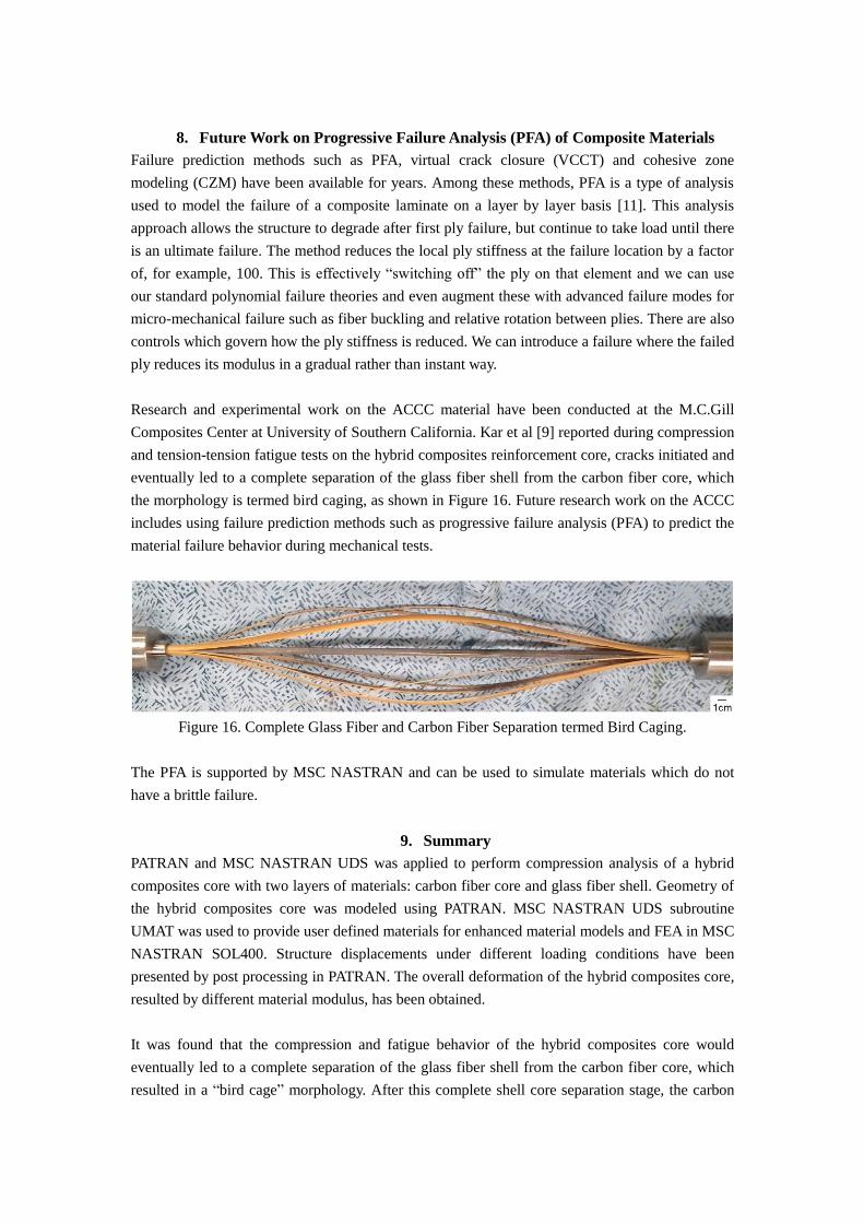
Research and experimental work on the ACCC material have been conducted at the M.C.Gill
Composites Center at University of Southern California. Kar et al [9] reported during compression
and tension-tension fatigue tests on the hybrid composites reinforcement core, cracks initiated and
eventually led to a complete separation of the glass fiber shell from the carbon fiber core, which
the morphology is termed bird caging, as shown in Figure 16. Future research work on the ACCC
includes using failure prediction methods such as progressive failure analysis (PFA) to predict the
material failure behavior during mechanical tests.
Figure 16. Complete Glass Fiber and Carbon Fiber Separation termed Bird Caging.
The PFA is supported by MSC NASTRAN and can be used to simulate materials which do not
have a brittle failure.
9. Summary
PATRAN and MSC NASTRAN UDS was applied to perform compression analysis of a hybrid
composites core with two layers of materials: carbon fiber core and glass fiber shell. Geometry of
the hybrid composites core was modeled using PATRAN. MSC NASTRAN UDS subroutine
UMAT was used to provide user defined materials for enhanced material models and FEA in MSC
NASTRAN SOL400. Structure displacements under different loading conditions have been
presented by post processing in PATRAN. The overall deformation of the hybrid composites core,
resulted by different material modulus, has been obtained.
It was found that the compression and fatigue behavior of the hybrid composites core would
eventually led to a complete separation of the glass fiber shell from the carbon fiber core, which
resulted in a “bird cage” morphology. After this complete shell core separation stage, the carbon

fiber core would support all of the applied loads. Future research work on ACCC include apply
failure prediction methods supported by PATRAN/MSC NASTRAN, such as progressive failure
analysis (PFA) to predict the ACCC material failure behavior during mechanical tests. MSC
NASTRAN and PATRAN serve as efficient tools for the modeling and the mechanical
load-displacement behavior prediction of hybrid composite materials.
10. Appendix
The MSC NASTRAN input files in this work and the descriptions are listed below:
Input Files Description
HybridComposite.bdf BDF input deck with SCA entry interfaces
HybridComposite.F90 User Defined Subroutine for UMAT, in Fortran
ext_umat.f MSC NASTRAN UDS UMAT, in Fortran
11. References
[1] North American Energy Reliability Corporation (2008). Long-Term Reliability Assessment.
[2] Alawar A (2005). Mechanical Behavior of a Composite Reinforced Conductor. PhD Thesis,
University of Southern California.
[3] The Aluminum Association. Bare Aluminum Wire and Cable Installation Practices.
[4] Boyd J, Speak S, Sheahen P. (1992). Galvanic Corrosion Effects on Carbon Fiber Composites
Results from Accelerated Tests. pg. 1184-98. 37th International SAMPE Symposium and
Exhibition. Anaheim, CA, USA.
[5] Alawar A, Bosze EJ, Nutt SR.(2005). 2005;20(3):2193-9. A Composite Core Conductor for
Low Sag at High Temperatures. IEEE Transactions on Power Delivery.
[6] Bosze EJ, Alawar A, Bertschger O, Tsai Y-I, Nutt SR. (2006). High-Temperature Strength and
Storage Modulus in Unidirectional Hybrid Composites. Composites Science and Technology.
2006;66(Compendex):1963-9.
[7] Tsai YI, Bosze EJ, Barjasteh E, Nutt SR. (2009) Influence of Hygrothermal Environment on
Thermal and Mechanical Properties of Carbon Fiber/Fiberglass Hybrid Composites. Composites
Science and Technology. 2009;69 (2009, The Institution of Engineering and Technology):432-7.
[8] Barjasteh E, Bosze EJ, Nutt SR. (2009). Thermal Aging of Fiberglass/Carbon-Fiber Hybrid
Composites. Comp A 2009; 40(12): 2038-2045.
[9] Kar N. (2012) Fatigue and Fracture of Pultruded Composite Rods Developed for Overhead
Conductor Cables. PhD Thesis, University of Southern California.
[10] MSC NASTRAN QRG. 4-24-2013.
[11] Andrew Main (2013). Use of Finite Element Analysis to Create Robust Composite Designs --
Going Beyond First Ply Failure. MSC Software Solution Paper Collection.
Recommended


![Coupled thermomechanical analisys of electrofusion ...pages.mscsoftware.com/rs/mscsoftware/images/coes_october6[1].pdfCoupled thermomechanical analisys of electrofusion fittings](https://img.dokumen.tips/doc/110x75/5adcf8f57f8b9a9d4d8c7bc7/coupled-thermomechanical-analisys-of-electrofusion-pages-1pdfcoupled-thermomechanical.jpg)