Anatomy of Corporate Borrowing Constraints∗
Chen Lian1 and Yueran Ma2
1Massachusetts Institute of Technology2Harvard University
October 31, 2017
Abstract
We investigate borrowing constraints of non-financial firms. We find that 20% of US
non-financial corporate debt by value is collateralized by specific physical assets (“asset-
based lending” in creditor parlance), while 80% is not tied to the liquidation value of
physical assets, and is based predominantly on cash flows from firms’ operations (“cash
flow-based lending”). A standard form of borrowing constraint restricts a firm’s total
debt as a function of cash flows measured using operating earnings (“earnings-based
borrowing constraints,” or EBCs). The centrality of cash flows in corporate borrowing
has several implications. First, cash flows in the form of operating earnings relax EBCs,
and enable firms to both borrow and invest more. This mechanism also reveals a new
channel of firms’ investment sensitivity to cash flows, one that arises from cash flows’
direct impact on borrowing constraints, rather than effects on internal funds. Second,
as corporate borrowing overall does not rely heavily on physical assets such as real
estate, firms could be less vulnerable to collateral damage from property price shocks.
In the Great Recession, for example, property price declines did not significantly affect
major US non-financial firms’ borrowing and investment through collateral damage.
Finally, results in the US contrast with those in Japan, where corporate borrowing
historically emphasizes physical assets.
∗We are grateful to Daron Acemoglu, Marios Angeletos, Ricardo Caballero, John Campbell, EmmanuelFarhi, Fritz Foley, Xavier Gabaix, Ed Glaeser, Robin Greenwood, Sam Hanson, Bengt Holmstrom, VictoriaIvashina, Song Ma, James Poterba, David Scharfstein, Andrei Shleifer, Alp Simsek, Jeremy Stein, DavidThesmar, Ivan Werning, Chunhui Yuan, Yao Zeng, and seminar participants at Harvard and MIT for veryhelpful suggestions. We are also thankful to finance and legal professionals Sarah Johnson, ChristopherMirick, Andrew Troop, Marc Zenner, and especially Kristin Mugford for sharing their knowledge. Firstdraft: May 2017.
1 Introduction
Constraints on firms’ ability to borrow play a critical role in economic analyses. What
determines these borrowing constraints? In some work, firms’ borrowing depends on cash
flows from operations and investment (Townsend, 1979; Stiglitz and Weiss, 1981; Holmstrom
and Tirole, 1997). More recently, the spotlight fell on the liquidation value of physical assets
that firms can pledge as collateral. This perspective has shaped theories in finance and
macroeconomics (Hart and Moore, 1994; Shleifer and Vishny, 1992; Kiyotaki and Moore,
1997; Bernanke, Gertler, and Gilchrist, 1999; Brunnermeier and Sannikov, 2014).
In this paper, we collect detailed data and empirically investigate borrowing by non-
financial firms in the US. We show that large US non-financial firms primarily borrow based
on cash flows from their operations (“cash flow-based lending” in creditor parlance), rather
than the liquidation value of physical assets (“asset-based lending”). A standard form of
borrowing constraint restricts a firm’s total debt as a multiple of a specific measure of cash
flows, namely operating earnings.1 We refer to this type of constraint as “earnings-based
borrowing constraint” or EBC.
The prevalence of cash flow-based lending and EBCs has several implications, which we
document empirically. First, they shape how cash flows affect borrowing and investment.
Cash flows in the form of operating earnings relax EBCs, and enable firms to both borrow
and invest more. This mechanism suggests a new channel for investment sensitivity to cash
flows: cash flows do not just increase internal funds; those in the form of operating earnings
also directly relax borrowing constraints. Moreover, with EBCs, the type of “cash flow”
matters: when a firm gets more cash receipts that do not count towards operating earnings,
EBCs are not relaxed, but internal funds rise and substitute out borrowing in the data.
Second, as corporate borrowing does not rely heavily on physical assets, large US firms’
sensitivity to collateral value, such as the value of real estate assets, could be diminished.
This low sensitivity may dampen asset price feedback type of financial acceleration through
firms’ balance sheets (Kiyotaki and Moore, 1997; Bernanke, Gertler, and Gilchrist, 1999), and
helps illuminate the transmission of shocks in crises. In the Great Recession, for instance,
we do not find that property price drops significantly affected major non-financial firms’
borrowing and investment through collateral damage.
Finally, we contrast the US with Japan, where corporate borrowing historically empha-
sizes physical assets (particularly real estate) given different legal infrastructure and lending
traditions. The results are the opposite of what we find in the US.
We begin by assembling detailed data on corporate debt, which integrates information
1In particular, earnings before interest, taxes, depreciation, and amortization (EBITDA), over the pasttwelve months. In this paper, we use the term “operating earnings” to refer to EBITDA.
1
from a number of databases (e.g. CapitalIQ, FISD, SDC, DealScan, ABL Advisors, Compu-
stat, Flow of Funds, SBA, Call Reports) and from hand collected data. The first part of our
data focuses on the collateral structure of debt, which covers individual debt for the majority
of public non-financial firms since 2002, as well as aggregate estimates for the non-financial
corporate sector. The second part of our data focuses on debt limit requirements and sources
of these restrictions. The data helps us document two main facts that point to the central
role of cash flows in corporate borrowing in the US.
First, borrowing against cash flows accounts for the majority of US non-financial cor-
porate debt. Specifically, 20% of corporate debt is collateralized by specific physical assets
(e.g. real estate, inventory, equipment, receivables, what creditors usually refer to as “asset-
based lending”), both in terms of aggregate dollar amount outstanding and for a typical
large non-financial firm (assets above Compustat median). The remaining 80% is not tied to
specific physical assets, and creditors’ payoffs (in both ordinary course and bankruptcy) are
driven by cash flows from continuing operations (what creditors refer to as “cash flow-based
lending”).2 The composition of corporate debt suggests that the liquidation value of physical
assets might not be the defining constraint for large US firms.
Second, borrowing constraints commonly rely on a specific measure of cash flows. They
stipulate that a firm’s total debt or debt payments cannot exceed a multiple of EBITDA
(earnings before interest, taxes, depreciation and amortization) in the past twelve months.
These EBCs restrict total debt at the firm level, rather than the size of a particular debt
contract. A primary source of EBCs is financial covenants in cash flow-based loans and
bonds. Those in loans monitor compliance on a quarterly basis, so the constraint is relevant
not just for issuing new debt, but also for maintaining existing debt. Among large public non-
financial firms, around 60% have earnings-based covenants explicitly written in their debt
contracts. Given contracting constraints, creditors focus on current EBITDA as a principal
metric of cash flow value, which is informative as well as observable and verifiable.
Corporate borrowing based on cash flows is not always the norm. Its feasibility and
practicality rely on legal infrastructure (e.g. accounting, bankruptcy laws, court enforcement)
and on firms generating sufficient cash flows. Once these conditions are met, cash flow-based
lending can be more appealing than pledging specific assets, as most corporate assets are
specialized, illiquid, or intangible. These factors shape several variations across firm groups,
which we revisit later to examine firm behavior under different forms of corporate borrowing.
First, cash flow-based lending is less common among small firms, given their low profits (if
not sustained losses) and higher likelihood of liquidation: for small public firms, the median
2The physical assets in asset-based lending are analogous to “land” in Kiyotaki and Moore (1997). Cashflows from firms’ operations in cash flow-base lending are analogous to “fruit” in Kiyotaki and Moore (1997).Bankruptcies for cash flow-based debt are primarily resolved through Chapter 11, which focuses on goingconcern cash flow value instead of liquidation value of specific physical assets.
2

share of cash flow-based lending is less than 10%; fewer than 15% of small firms are subject
to earnings-based covenants. Second, cash flow-based lending and EBCs are similarly less
prevalent among low profit margin firms. Third, while cash flow-based lending dominates in
large firms across most industries, airlines and utilities are two exceptions, where firms have a
substantial amount of standardized transferable assets (aircraft and power generators) and a
significantly higher share of asset-based lending.3 Finally, the predominant form of corporate
borrowing may vary across countries given differences in institutional environments, which
we illustrate using the example of Japan.4
Recognizing the key role of cash flows in corporate borrowing in the US sheds light on
several issues. To begin, with cash flow-based lending and EBCs, cash flows in the form of
operating earnings relax borrowing constraints, and enable firms to both borrow and invest
more. This mechanism offers a new channel for how financial variables affect borrowing
constraints and firm outcomes, which is distinct from the influence of physical collateral
commonly studied in the macro-finance literature. The mechanism also points to a new
venue for investment sensitivity to cash flows. It contrasts with the traditional framework
in corporate finance analyses (Fazzari, Hubbard, and Petersen, 1988; Froot, Scharfstein, and
Stein, 1993; Kaplan and Zingales, 1997): following the pecking order idea (Myers and Majluf,
1984), the main function of cash flows is to increase internal funds, which boost investment
but substitute out external financing as long as investment has diminishing marginal returns.
Our account of corporate borrowing yields three predictions. First, all else equal, in the
presence of EBCs, higher cash flows in the form of operating earnings (EBITDA) relax bor-
rowing constraints, and crowd in borrowing as well as investment. Second, holding EBITDA
fixed, higher net cash receipts do not directly relax EBCs, but increase internal funds, which
can boost investment but may decrease borrowing. Third, the key role of EBITDA for bor-
rowing and investment is not present among firms not bound by EBCs (e.g. unconstrained
firms and firms where asset-based lending prevails).5
Our empirical tests begin with a baseline regression that mimics a traditional invest-
ment regression, with a few key modifications. First, we analyze both debt issuance and
investment activities as outcome variables, to explore how cash flows affect firms through
external borrowing. Second, we analyze the role of EBITDA, which directly enters firms’
borrowing constraints, and separate it from internal funds (cash receipts) to further inves-
3The high share of asset-based lending in airlines is consistent with Benmelech and Bergman (2009) andBenmelech and Bergman (2011), who thoroughly analyze the collateral channel in this industry.
4The legal bases of corporate borrowing reflect the insights of research on law and finance (La Porta,Lopez-de Silanes, Shleifer, and Vishny, 1997, 1998; Djankov, Hart, McLiesh, and Shleifer, 2008).
5In addition, this observation offers a new perspective for the debate about whether more constrainedfirms are more sensitive to cash flows (Kaplan and Zingales, 1997, 2000; Fazzari, Hubbard, and Petersen,2000): among plausibly more constrained small firms, cash flow-based lending and EBCs are uncommon,which removes one possible channel of cash flow sensitivity (if cash flows are measured based on earnings,which is typical in the literature).
3

tigate the borrowing channel. Third, we start with firms where EBCs are most important,
specifically large firms with earnings-based covenants, and then analyze several firm groups
where EBCs are less relevant. We find that among large firms with EBCs, all else equal,
a one dollar increase in EBITDA is on average associated with a 27 cents increase in net
long-term debt issuance. Investment activities increase by about 15 cents. These patterns do
not exist among other firm groups not bound by EBCs (e.g. unconstrained firms and firms
that primarily use asset-based lending, such as small firms, low margin firms, airlines and
utilities, Japanese firms, etc.) On the other hand, holding EBITDA constant, a one dollar
increase in net cash receipts on average leads to a 5 cents increase in investment but a 10
cents reduction in net long-term debt issuance.
We further verify the role of operating earnings by studying a natural experiment that
generates exogenous variations in earnings, due to changes in an accounting rule (Financial
Accounting Standards Board’s rule SFAS 123(r)). Before the adoption of this rule, firms’
option compensation expenses do not formally count towards earnings, while the new rule
requires their inclusion. Thus the rule affects the calculation of operating earnings, but
does not directly affect firms’ cash positions or economic fundamentals. As prior research
demonstrates, contracting frictions make it hard to neutralize changes in accounting rules,
and they tend to have a significant impact on borrowers through debt covenants (Frankel,
Lee, and McLaughlin, 2010; Moser, Newberry, and Puckett, 2011; Cohen, Katz, and Sadka,
2012; Shroff, 2017). We instrument operating earnings after the adoption of SFAS 123(r),
using average option compensation expenses in three years prior to the rule announcement.
We find strong first-stage results among all firm groups, but only second stage results on
debt issuance and investment for firms bound by EBCs. The findings attest to the influence
of operating earnings on borrowing constraints and firm outcomes on the margin.
While lending practices in the US contribute to the sensitivity of corporate borrowing
and investment to cash flows (especially earnings), they may diminish the sensitivity to the
value of physical assets such as real estate (which accounts for only 7% of US non-financial
corporate debt by value). Using both traditional estimates of firm real estate value and
hand collected property-level data from company filings, we find that US large non-financial
firms’ borrowing has relatively small sensitivity to real estate value, concentrated in asset-
based debt. For cash flow-based debt, the sensitivity is absent, if not negative and offsetting
the response of asset-based debt. Overall, borrowing increases by three to four cents on
average for a one dollar increase in property value, consistent with findings by Chaney, Sraer,
and Thesmar (2012). The magnitude is considerably smaller than the impact of operating
earnings among US large firms.
This observation helps understand aspects of the Great Recession and the transmission of
property value declines in this crisis. By exploiting firms’ differential exposures to property
4
price declines, we do not find that the drop in the value of real estate assets had a significant
impact on borrowing and investment.6 Such diminished sensitivity may decrease the scope of
asset price feedback type of financial acceleration through firms’ balance sheets. Meanwhile,
the decline in corporate earnings did have a significant impact through EBCs, which accounts
for roughly 10% of the drop in debt issuance and capital expenditures among public firms
from 2007 to 2009. The magnitude is meaningful but not catastrophic, in line with the view
that the US Great Recession is a crisis centered around households and banks rather than
major non-financial firms.
The story in the US finds its antithesis in Japan. Unlike the US where cash flow-based
lending prevails, Japan historically lacked legal infrastructure for such lending practices,
and instead developed a corporate lending tradition focused on physical assets, especially
real estate. We show that Japanese firms do not display sensitivity of debt issuance to
operating earnings. Japanese firms are, however, very sensitive to declines in the value of
real estate assets during the Japanese property price collapse in the early 1990s. Gan (2007)
shows the drop in Japanese firms’ property value had a substantial and long-lasting impact
on their borrowing and investment. Using the specification of Gan (2007), we do not find
similar results among US firms during the Great Recession. Recognizing the differences in
institutional environments and corporate borrowing practices helps to synthesize distinct
evidence across different countries.
The domain of our study is non-financial corporations. Financial institutions’ borrowing
constraints may take different forms, and tie to the liquidation value of securities pledged as
collateral. The ensuing fire-sale amplifications have been thoroughly analyzed (Shleifer and
Vishny, 1997; Gromb and Vayanos, 2002; Coval and Stafford, 2007; Garleanu and Pedersen,
2011), and map closely to models of asset price feedback (Shleifer and Vishny, 1992; Kiyotaki
and Moore, 1997; Bernanke, Gertler, and Gilchrist, 1999; Brunnermeier and Sannikov, 2014).
Constraints for small businesses may also be different, and significantly dependent on real
estate value, making them highly exposed to property price fluctuations through collateral
value (Adelino, Schoar, and Severino, 2015; Schmalz, Sraer, and Thesmar, 2017).
Related Literature. Our paper relates to several strands of research. First, an impor-
tant macro-finance literature offers theoretical insights about firms’ borrowing constraints
and their economic significance (Hart and Moore, 1994, 1998; Shleifer and Vishny, 1992; Kiy-
otaki and Moore, 1997; Bernanke, Gertler, and Gilchrist, 1999; Holmstrom and Tirole, 1997;
Rampini and Viswanathan, 2013; Diamond, Hu, and Rajan, 2017). These analyses motivate
our empirical investigation. We show the prevalence of asset-based versus cash flow-based
lending, the pervasiveness of earnings-based borrowing constraints, and variations across
6Our result is consistent with indirect evidence from Mian and Sufi (2014) and Giroud and Mueller (2017),and with their proposition that the main effect of the property price collapse was to impair household demand.
5

firms and countries. We also document that different forms of corporate borrowing have
distinct impact on financial and macroeconomic outcomes.
Second, our work builds on research on corporate debt. Rauh and Sufi (2010) highlight
the importance of studying debt composition and heterogeneity. We perform a systematic
analysis of asset-based and cash flow-based lending, and investigate their economic impact.
We also build on studies of financial covenants (Chava and Roberts, 2008; Roberts and
Sufi, 2009; Nini, Smith, and Sufi, 2009, 2012; Ivashina, 2009; Demerjian, 2011; Murfin, 2012;
Acharya, Almeida, Ippolito, and Perez-Orive, 2014; Falato and Liang, 2016; Becker and
Ivashina, 2016) to examine the enforcement of earnings-based borrowing constraints. We
apply insights from corporate debt analyses to better understand questions in macro-finance.
Third, our investigation of borrowing constraints sheds new light on how cash flows
affect corporate borrowing and investment. Cash flows in the form of operating earnings,
by directly relaxing borrowing constraints, play a key role in crowding in borrowing and
investment. This mechanism points to a distinct channel for the widely studied issue of
investment sensitivity to cash flows (Fazzari, Hubbard, and Petersen, 1988; Hoshi, Kashyap,
and Scharfstein, 1991; Froot, Scharfstein, and Stein, 1993; Blanchard, Lopez-de Silanes, and
Shleifer, 1994; Kaplan and Zingales, 1997; Almeida, Campello, and Weisbach, 2004; Rauh,
2006). We further lay out the differences among different types of cash flows, different
firms, and different countries. Sufi (2009) studies earnings-based covenants (cash flow-based
financial covenants in his paper) to analyze firms’ access to bank lines of credit. He shows
these requirements limit low cash flow firms’ ability to use credit lines, which tightens their
financial constraints and makes them more reliant on cash for liquidity management.
Finally, our investigation helps understand firms’ vulnerability to property price shocks
and features of the Great Recession. Building on previous research (Chaney, Sraer, and
Thesmar, 2012; Cvijanovic, 2014; Demirci, Gurun, and Yonder, 2017), we find US firms’
borrowing and investment exhibit some sensitivity to real estate value. However, the sensi-
tivity is concentrated in asset-based debt, is less pronounced than the sensitivity to earnings,
and appears sufficiently modest to avert severe impact of collateral damage. We also connect
to studies of the Great Recession, and use firm property holdings data to further unpack
the transmission of property price declines. Our findings illuminate the role of firms’ bal-
ance sheets in the crisis, and support the centrality of households’ and financial institutions’
balance sheet impairment in the US experience (Mian and Sufi, 2014; Giroud and Mueller,
2017; Chodorow-Reich, 2014; Chodorow-Reich and Falato, 2017).
The rest of the paper is organized as follows. Section 2 documents the features of corpo-
rate borrowing in the US. Section 3 studies the impact of cash flows on corporate borrowing
and investment; Section 4 studies the impact of property collateral value and implications
for the transmission of shocks in the Great Recession. Section 5 concludes.
6

2 Corporate Borrowing in the US
In this section, we document two facts about corporate borrowing in the US. First, in the
aggregate and among large firms, the majority of corporate debt is based on cash flows from
firms’ operations (“cash flow-based lending”), as opposed to the liquidation value of specific
physical assets (“asset-based lending”). Second, in this setting, a prevalent form of borrowing
constraint is tied to a specific measure of cash flows, namely operating earnings, which we
refer to as earnings-based borrowing constraints (EBCs). At the end, we discuss determinants
of these practices and variations across firms. We then overview the implications of these
facts, which we explore in Sections 3 and 4.
To study these facts, we collect and integrate data from a number of sources. We utilize
many sources because corporate debt information is often scattered: each dataset covers
some specific types of debt, or some specific debt attributes. Combining many sources also
allows us to cross check results using different datasets and enhance accuracy. The first part
of our data focuses on debt composition, and uses key features such as collateral structure
to categorize debt into asset-based and cash flow-based lending. We provide aggregate es-
timates for the non-financial corporate sector (using Flow of Funds, bond aggregates from
FISD, large commercial loan aggregates from SNC, DealScan, and ABL Advisors, small busi-
ness loan aggregates from SBA and Call Reports, capital lease estimates from Compustat,
among others). We also perform firm-level analyses for most public firms since 2002 (using
primarily debt-level descriptions from CapitalIQ, supplemented with bond data from FISD,
loan data from DealScan, and additional debt information from SDC). The second part of
our data focuses on EBCs. We record legally binding constraints specified in firms’ debt con-
tracts, including loans (DealScan) and bonds (FISD); we also document indications of such
constraints imposed by market norms. We verify that we accurately capture the sources of
these constraints by additionally scraping firms’ annual report filings, and manually reading
firms’ disclosures in filings for a sample year of 2005.
2.1 Stylized Facts
2.1.1 Fact 1: Prevalence of Cash Flow-Based Lending
We first study the composition of corporate borrowing, and document the prevalence of
asset-based lending and cash flow-based lending.
Asset-Based Lending
In asset-based lending, the debt is collateralized by specific assets (most commonly real
estate, inventory, receivable, and certain types of machinery and equipment). Creditors
7
have claims against the underlying assets pledged as collateral, and their payoffs in default
depend on the liquidation value of the collateral. Each debt typically has a size limit based
on the liquidation value of the specific assets pledged as collateral for that debt. The limit is
enforced throughout the duration of the debt in some cases (e.g. revolving credit lines based
on working capital), and enforced only at issuance in others (e.g. commercial mortgage).
In the data, we classify a debt as asset-based if one of the following criteria is met: a)
we directly observe one of the features above (e.g. collateralized by specific assets or have
borrowing limits tied to them); b) the debt belongs to a debt class that is usually asset-based
(e.g. secured revolving line of credit, finance company loans, capital leases, small business
loans, etc.), or it is labeled as asset-based; c) all other secured debt that does not have
features of cash flow-based lending (discussed below) to be conservative (i.e. we may over-
estimate rather than under-estimate the amount of asset-based lending). We leave personal
loans (from individuals, directors, related parties, etc.), government loans, and miscellaneous
loans from vendors and landlords unclassified (neither asset-based nor cash flow-based); their
share is less than one percent in the aggregate, but can be more significant among certain
small firms. Appendix B provides a detailed description of the categorization procedure.
Among total US non-financial corporate debt outstanding, we find that asset-based lend-
ing accounts for roughly 20% of debt by value, of which around 7% are mortgages (secured
by real estate) and the rest are other asset-based loans (secured by receivable, inventory,
equipment, etc.). For individual firms, results are similar in large non-financial firms: among
the larger half of public firms (by assets), the median share of asset-based lending is 12%;
among rated firms, the median share is 8%.7
Cash Flow-Based Lending
In cash flow-based lending, the debt is not tied to specific physical assets; creditors’ payoffs
(in ordinary course and in bankruptcy) depend primarily on cash flows from firms’ operations,
as opposed to the liquidation value of physical assets.8 Examples include corporate bonds
and a significant share of corporate loans such as most syndicated loans. The debt is often
unsecured; the ones that are secured are secured by a lien on the entire corporate entity
or by equity of the borrower (rather than specific physical assets), and the value of this
form of collateral in bankruptcy is determined based on the cash flow value from continuing
7Rauh and Sufi (2010) study debt structure of 305 rated firms, and provide firm-level data for debtoutstanding by debt class (e.g. public bonds, revolvers, mortgages). With assumptions about whether eachdebt class is asset-based or cash flow-based (e.g. public bonds are cash flow-based, mortgages are asset-based,revolvers are a mix), we can get another estimate of debt composition. This alternative estimate and ourfirm-level calculations match closely; the median level matches one for one for firm-years in both samples.
8In Chapter 11 bankruptcy, which is typical for firms using cash flow-based lending, the payoffs are drivenby the cash flow value from continuing operations (“going-concern” value). In the rare cases of ending upin Chapter 7, these debt generally have minimal recovery. Thus creditors’ payoffs overall are not tied to theliquidation value of physical assets. Using bankruptcy filing data from CapitalIQ (see Iverson (2017) for adetailed description), about 90% of large public firms’ bankruptcies are resolved through Chapter 11.
8

operations (Gilson, 2010). The key function of having security is to establish priority in
bankruptcy and restructuring (US bankruptcy laws treat secured creditors as one class who
have priority over unsecured creditors), not to liquidate the collateral. In cash flow-based
lending, creditors do not focus on the liquidation value of physical assets (which are not
key determinants of their payoffs or debt capacity); they focus instead on assessing and
monitoring firms’ cash flows.
In the data, we categorize a debt as cash flow-based if one of the following criteria is
met: a) it is unsecured, or secured by substantially all assets/pledge of stock and does not
have any features of asset-based lending; b) the debt belongs to a debt class that is primarily
cash flow-based (e.g. corporate bonds other than asset-backed bonds and industrial revenue
bonds, term loans in syndicated loans), or it is labeled as cash flow-based. Appendix B
provides a detailed explanation of the categorization.
Among total US non-financial corporate debt outstanding, cash flow-based lending ac-
counts for about 80% of debt by value, of which 50% are corporate bonds and 30% are cash
flow loans. At the firm level, results are similar in large non-financial firms: among the
larger half of public firms, the median share of cash flow-based lending is 83%; among rated
firms, the median share is 89%. In Figure 1 Panel A, we also aggregate up firm-level data
and plot the share of cash flow-based and asset-based lending by year among large public
non-financial firms: the share of cash flow-based lending is consistently 80% and that of
asset-based lending is consistently 20%.
In Appendix B, we further test and verify that cash flow-based debt does not have indirect
positive dependence on the value of specific physical assets. Table A3 shows the amount of
asset-based debt a firm has is positively correlated with the value of physical assets, whereas
the amount of cash flow-based debt is not (if anything, the correlation is typically negative).
Taken together, cash flow-based lending accounts for the majority of US corporate debt,
in the aggregate and among large firms. In the following, we document a prevalent form of
borrowing constraints in this setting.
2.1.2 Fact 2: Prevalence of Earnings-Based Borrowing Constraints
The second stylized fact shows that, in the context of cash flow-based lending, a common
form of borrowing constraint stipulates debt limits based on a specific measure of cash
flows, specifically operating earnings. We refer to this type of constraints as earnings-based
borrowing constraints (EBCs). EBCs follow two main specifications. The first is a limit on
the ratio of a firm’s debt to its operating earnings:
bt ≤ φπt (1)
9
where πt is the firm’s annual operating earnings, bt is the firm’s debt, and φ is the maximum
ratio.9 The second is a limit on the minimum amount of earnings relative to debt payments:
bt ≤θπtrt
(2)
where rtbt is interest payments, and θ is the minimum coverage ratio.
EBCs have several features. First, the constraint applies at the firm level: both earnings
πt and the amount of debt bt (or debt payments rtbt) are those of the borrowing firm. This
is different from, for instance, the “loan-to-value” constraint of a mortgage that applies only
to the size of that particular loan. At a given point in time, a firm may face earnings-based
borrowing constraints from different sources, as we discuss shortly. Each of these constraints
has a parameter φ or θ, and the tightest one binds first.10 Second, the commonly used
measure for πt is EBITDA (earnings before interest, tax, depreciation, and amortization),
over the past twelve months. As the name indicates, EBITDA excludes taxes and interest
expenses. It also excludes non-operating income and special items (e.g. windfalls, natural
disaster losses, earnings from discontinued operations). Third, EBCs apply not just when
firms issue new debt; they can also affect the maintenance of existing debt. Even if a firm
is not issuing new debt, if its earnings decline significantly, it may need to reduce debt to
comply with these constraints imposed by existing debt.
Below we discuss the sources and enforcement of EBCs.
Earnings-Based Debt Covenants
An important source of EBCs is financial covenants in debt contracts. Covenants are
legally binding provisions in debt contracts that specify restrictions on borrowers; financial
covenants are one type of covenants limiting borrowers’ financial conditions, assessed based
on financial statements. Violations of covenants trigger “technical defaults,” in which case
creditors have legal power to accelerate payments or terminate the credit agreement. While
such actions are infrequent, creditors use the bargaining power to request fees, increase bor-
rowing costs, restrict borrowers’ financial decisions, and replace management teams (Roberts
and Sufi, 2009; Nini, Smith, and Sufi, 2009, 2012). Covenant violations prompt transfers of
control rights to creditors, and incur significant costs to borrowers.
A common type of financial covenants specify debt limits as a function of EBITDA, which
we refer to as earnings-based covenants. They follow the forms in Equations (1) and (2), and
share the feature discussed above that the debt limits are at the firm level (so a firm is subject
to constraint as long as one of its debt contracts contains such covenants). Earnings-based
9The debt-to-earnings ratio is a central concept to creditors: in credit agreements, lenders typically usethe term “leverage ratio” to refer to the debt-to-earnings ratio (rather than the debt-to-assets ratio).
10In Equations (1) and (2), we do not specify a time subscript t for the parameters φ or θ. At the firmlevel, the overall tightness of EBCs may vary over time (as old constraints get replaced by new ones, etc.).
10

covenants can be found in both corporate loans and bonds. Loans monitor compliance on a
quarterly basis throughout their duration (“maintenance tests”); thus continuous compliance
is relevant for the maintenance of existing loans, connected to the third feature discussed
above. Bonds monitor compliance only when borrowers take certain actions such as issuing
new debt (“incurrence tests”), and are relevant for new debt issuance.
We study earnings-based covenants using data from three sources: DealScan for com-
mercial loans, FISD for corporate bonds, and scraped and hand collected data from annual
reports. DealScan is the most widely used dataset for corporate loans, with comprehensive
coverage (Strahan, 1999; Bradley and Roberts, 2015), especially for large syndicated loans
(it may not cover small bilateral loans, personal loans, mortgage loans, finance company
loans). As we verify below, commercial loans are the primary type of loans with earnings-
based covenants. DealScan provides data on covenant specifications and thresholds; Table
A5 in Appendix C.1 lists the main specifications and the corresponding accounting variables
compiled by Demerjian and Owens (2016). FISD is a comprehensive dataset for corporate
bonds, with information on the type of covenant but not the covenant threshold. Finally,
to check the comprehensiveness of data from DealScan and FISD and better understand the
sources of earnings-based covenants, we scrape firms’ annual report filings, and manually
read covenant-related discussions for the sample year of 2005. Our sample covers US public
non-financial firms from 1996 to 2015, as covenant data is relatively sparse prior to 1996.
Sources. Earnings-based covenants primarily come from debt that belongs to cash flow-
based lending. To get a comprehensive picture of the sources of earnings-based covenants, we
read firms’ filings for the sample year of 2005. Among mentions of earnings-based covenants
in filings, 90% come from debt that belongs to cash flow-based lending (or is packaged with
cash flow-based debt11), such as cash flow-based commercial loans and corporate bonds.
Less than 10% come from other types of loans (e.g. mortgage loans, equipment loans, capital
leases, etc.). These results also verify the validity of using DealScan and FISD data for
systematic analyses of earnings-based covenants.
Prevalence. Figure 1 Panel B merges data from DealScan and FISD with Compustat,
and shows that earnings-based covenants are prevalent among large firms. Of all large
public firms, about 50% to 60% have earnings-based covenants in their debt contracts.12
If we add mentions of earnings-based covenants scraped from firms’ filings, the share of
11Commercial loans are typically organized in a package that shares the same covenants: the packagecommonly contains a revolving credit line, which can be asset-based (secured by inventory and receivable,with borrowing limits based on eligible collateral), and cash flow-based term loans. Thus the revolving linesare also subject to earnings-based covenants although we categorize them into asset-based lending.
12Examples include AAR Corp, AT&T, Barnes & Noble, Best Buy, Caterpillar, CBS Corp, Comcast,Costco, Disney, FedEx, GE, General Mills, Hershey’s, HP, IBM, Kohl’s, Lear Corp, Macy’s, Marriott, Merck,Northrop Grumman, Pfizer, Qualcomm, Rite Aid, Safeway, Sears, Sprint, Staples, Starbucks, StarwoodHotels, Target, Time Warner, US Steel, Verizon, Whole Foods, Yum Brands, among many others.
11
large non-financial firms with EBCs increases by another 5% per year, but the scraped data
could contain false positives.13 Large firms as a whole account for more than 90% of the
sales, investment, and employment of all public firms. Those with earnings-based covenants
account for about 60%. Some large firms do not have earnings-based covenants written in
their debt contracts because they currently have little debt and are far from the constraints
(e.g. Apple nowadays). Nonetheless, the constraint still exists and they are likely to have
explicit debt covenants if the debt level is higher (e.g. Apple fifteen years ago).
In addition to earnings-based covenants, there are a few other types of financial covenants,
mostly in corporate loans. These covenants are less prevalent in comparison, as we show in
Internet Appendix A1.14
Violations and Tightness. We also examine consequences of covenant violations and
covenant tightness. Here we focus on loan covenants, for which we have some information
about the specific covenant specifications and thresholds. Figure 2 plots firm-level debt
growth in year t + 1 against distance to the covenant threshold at the end of year t.15 It
shows that debt growth is on average positive when firms are in compliance (to the right of the
dashed line), but becomes negative once firms break the covenants.16 The evidence suggests
that earnings-based covenants serve as effective borrowing constraints. It is consistent with
previous research that provides in-depth analyses of covenant violations and how they restrict
corporate borrowing (Chava and Roberts, 2008; Roberts and Sufi, 2009). Figure 3 shows
that firms bunch near the constraint, indicating violations are costly and borrowers try to
avoid them. For tightness, every year around 10% of large firms with DealScan loans break
the thresholds set by earnings-based covenants; another 10% to 15% are within 0.5 standard
deviations of the thresholds. The statistics are consistent with prior work (Nini, Smith, and
13For instance, the covenant mentioned in the filing may be about a loan that is already paid off. Firmsmay also discuss, for example, “interest coverage ratio” and “leverage ratio” in general, not in relations tocovenant requirements. These cases are hard to cleanly tease out in the scraping process.
14Other financial covenants have two main forms. One type specifies an upper bound on book leverage,or relatedly a lower bound on book equity (book net worth). Since book equity is closely related to theaccumulation of past earnings, this can be broadly viewed as a variant of EBC. The popularity of this typeof covenant has declined in the past twenty years for several reasons that we discuss in the Internet AppendixSection A1. Currently the prevalence of the book leverage/net worth covenants is less than a third of theprevalence of earnings-based covenants, and violations are uncommon. The other type of financial covenantspecifies limits on the ratio of current assets to current liabilities. These covenants are distinct from EBCs.
15As shown in Table A5, earnings-based covenants have several variants. Firms sometimes have more thanone type of these covenants; different firms may also have different types. For a uniform measure of distance,we first compute the minimum amount of earnings (πit) required such that the firm is in compliance with allof its earnings-based covenants (given the current level of debt). We then compute the difference betweenthe minimum earnings required (πit) and the actual earnings (πit), scaled by lagged assets. We normalizethis distance by the standard deviation of ROA in the firm’s 2-digit SIC industry.
16DealScan’s data allows us to observe the threshold set by the initial credit agreement (at loan issuance).Firms may subsequently renegotiate with lenders to amend credit agreements and relax covenants, and theseamendments may not be fully captured by DealScan’s data. Thus the actual threshold may end up beingslightly looser than the ones in our data. Nevertheless, we already observe a pause in debt growth once theinitial threshold is reached.
12

Sufi, 2012). The constraints are tight and relevant.17
Other Earnings-Based Borrowing Constraints
The earnings-based borrowing constraints a firm faces are not limited to financial covenants.
The corporate credit market has important norms about debt relative to earnings: when a
firm wants to issue debt, it can be hard to surpass a reference level of debt to EBITDA ratio
lenders are accustomed to. This limit can be tighter than covenants in existing debt or in
the new debt (the covenants of the new debt, if there are any, are typically set in a way that
they will not be violated immediately). These earnings-based constraints at issuance are
especially relevant for non-investment grade firms, which are closer to the limit. Such firms
also commonly borrow from the leveraged loan market, where the reference debt to EBITDA
ratio is emphasized the most. We document the impact of these additional constraints in
Appendix C.2 using measures of the reference level in the leveraged loan market.
In sum, earnings-based borrowing constraints play an important role in US corporate
credit markets, and tie closely to the prevalence of cash flow-based lending. In Appendix D,
we provide formal models to analyze the contracting functions of earnings-based covenants in
cash flow-based lending, including incentive provision (Innes, 1990) and contingent transfer
of control rights (Aghion and Bolton, 1992). We also discuss why creditors focus on current
EBITDA: within contracting constraints, creditors use current EBITDA as a metric which is
informative about firm performance and cash flow value, as well as observable and verifiable.
EBITDA excludes windfalls to focus on cash flow generation by firms’ core businesses; it is
also available on a regular basis based on financial statements. Thus EBITDA has become a
standard, widely used metric, and evaluating borrowing constraints as multiples of EBITDA
has evolved to be a credit market norm.
2.1.3 Heterogeneity in Corporate Borrowing
Our previous discussions focus on large US non-financial firms. Corporate borrowing
based on cash flows is not always the norm. The primary form of borrowing varies across
large and small firms, in certain industries, and across countries, which we summarize below.
These variations are driven by three main factors that affect the feasibility and utilization
of cash flow-based lending: legal foundations, firms’ cash flow generating ability, and asset
specificity. First, the feasibility of lending and contracting based on cash flows relies on legal
infrastructure, including reliable financial accounting and auditing, as well as statues (espe-
cially bankruptcy laws) and court enforcement that ensure lending based on cash flows can
17The fraction of firms violating covenants or close to violation does not show strong cyclical patterns.This suggests that firms are not passive; they appear to actively adjust debt level and control their distanceto violation.
13

get paid back on average. With weak accounting, weak courts, or bankruptcy regimes that
tie creditors’ payoffs to the liquidation value of physical assets, cash flow-based lending could
be harder to pursue. Second, firms also need to be able to generate sufficient cash flows for
cash flow-based lending to be practical. Third, among firms that can access both asset-based
and cash flow-based lending, the relative utilization can depend on asset attributes. Most
large US firms have a small amount of standardized transferable assets that support low-cost
asset-based lending. The majority of assets, however, are specialized, illiquid, or intangible,18
and the US institutional environment makes cash flow-based lending more appealing.19 In
certain industries, particularly airlines and utilities, firms have a large share of standardized
transferable assets, which facilitate asset-based lending.
Variations in the US
Small Firms. Cash flow-based lending and EBCs are much less common among small
firms. The median share of cash flow-based lending is about 7% (while the median share of
asset-based lending for these firms is 61%; the rest are personal loans from individuals and
other miscellaneous borrowing). EBCs are found in only 12% of small firms (assets less than
Compustat median). The majority of small firms have little profits if not sustained losses
(Denis and McKeon, 2016).20 In addition, financial distress of small firms is more likely
to be resolved through liquidations (Bris, Welch, and Zhu, 2006; Bernstein, Colonnelli, and
Iverson, 2017), given the fixed costs of restructuring (e.g. legal and financial personnel) and
the uncertain prospects of small firms. This makes it harder for creditors to count on cash
flow value from continuing operations. With limited access to cash flow-based lending, small
firms rely significantly on physical assets to obtain credit.
Low Profitability Firms. Similar to the case of small firms, firms with low profitability
and low margins also have substantially lower shares of cash flow-based lending (higher shares
of asset-based lending), and lower prevalence of EBCs. Among low margin firms (profit
margin in the bottom half of all Compustat firms), the median shares of cash flow-based
lending and asset-based lending are 41% and 39% respectively, while among high margin
firms the median shares are 74% and 19% respectively.
Airlines and Utilities. Figures 4 shows corporate borrowing in different industries,
focusing on rated firms so that firms in different industry groups are comparable in size and
18This is consistent with the observation of Catherine, Chaney, Huang, Sraer, and Thesmar (2017) thatthe pledgeability of physical assets is low on average.
19For instance, Boeing’s aircraft production facilities generate high cash flows when producing Boeingaircraft, but the liquidation value of these assets could be very low. In such cases, borrowing againstcash flows would be more appealing than borrowing against specific physical assets in the US environment.Correspondingly, the debt is structured to focus on cash flows (e.g. extensive use of financial covenants),rather than enforcing creditors’ rights over specific physical assets.
20For instance, the median EBITDA to asset ratio among small Compustat firms is -0.01 (while thatamong large Compustat firms is 0.13).
14

capital market access. Most industries display similar patterns, with the exception of airlines
and utilities. In these two industries, even rated firms have a significant share of asset-based
lending and a relatively small share of cash flow-based lending. The prevalence of EBCs
is also lower. Airlines and utilities are special cases where firms have a large amount of
standardized transferable assets (aircraft and power generators) that facilitate asset-based
lending.
Cross-Country Variations
Across countries, lending practices may vary given different legal infrastructure (La Porta,
Lopez-de Silanes, Shleifer, and Vishny, 1997, 1998). In most developing countries, high qual-
ity accounting information can be a major hurdle. Among developed countries, differences
in accounting quality still exist but may not be large enough (especially among established
firms) to account for most of the variations. Differences in laws and practices regarding
financial distress seem more important. In the US, the tenet of Chapter 11 is to prevent
liquidations and preserve cash flow value from continuing operations (i.e. “going-concern
value”).21 In Chapter 11, creditors’ payoffs are determined by the cash flow value of the
firm, distributed according to priority (Gilson, Hotchkiss, and Ruback, 2000; Gilson, 2010).
Chapter 11 also has multiple provisions to facilitate the process (e.g. automatic stay, debtor-
in-possession, DIP financing22), which together make cash flow value central to creditors
and attenuate the role of physical collateral. In continental Europe, liquidations are more
common and bankruptcy procedures give more power to secured creditors (Djankov, Hart,
McLiesh, and Shleifer, 2008; Smith and Stromberg, 2004).23
In major developed countries, legal infrastructure and lending practices in Japan tradi-
tionally lie at the other end of the spectrum from the US. Prior to 2000, bankruptcy courts
in Japan were largely dysfunctional, due to limited court capacity and provisions that dis-
couraged companies from filing for bankruptcy protection. Without court supervision, it
is harder to contract on cash flow value and enforce corresponding payouts. In addition,
there are no stays that prevent creditors from seizing collateral and disrupting efforts for
reorganization. Thus, physical collateral that can be seized tends to be central. It is well
known that corporate lending in Japan historically focused on hard assets, and real estate is
especially popular (Gan, 2007; Peek and Rosengren, 2000; Tan, 2004). Rajan and Zingales
21Bernstein, Colonnelli, and Iverson (2017) provide detailed empirical evidence that the Chapter 11 re-structuring procedure prevents loss of value relative to the Chapter 7 liquidation procedure.
22The automatic stay prevents creditors from seizing collateral and other debt collection activities afterbankruptcy filing. Chapter 11 allows existing management teams to stay (debtor-in-possession) to increaseincentives for firms to file and conduct timely restructuring. Firms can also obtain additional high prioritydebt (DIP financing) to support continued operations and ameliorate debt overhang problems.
23In the US, the share of unsecured corporate debt, as one indicator for the prevalence of cash flow-basedlending, is fairly high, at around 50%. The figure is about 30% in the UK. It is less than 20% for Germany,France, and EU average, and similarly low for Japan.
15

(1995) also find that tangible assets have a significantly higher impact on firm leverage in
Japan compared to other G-7 countries. In Sections 3 and 4, we contrast our findings in the
US with results in Japan, which further illustrates the impact of different forms of corporate
borrowing constraints.
2.2 Implications
Section 2.1 highlights the prevalence of cash flow-based lending and EBCs among large
US non-financial firms. In Sections 3 and 4, we study how such practices shape the way
financial variables affect borrowing constraints and firm outcomes on the margin. In Section
3, we study how they affect the role of cash flows in corporate borrowing and investment. In
Section 4, we study the mirror image: how they affect the sensitivity of corporate borrowing
and investment to the value of physical assets, specifically real estate, and implications for
the transmission of shocks in the Great Recession.
3 Cash Flows, Corporate Borrowing, and Investment
In this section, we study how cash flow-based lending and EBCs shape the role of cash
flows in corporate borrowing and investment.
In the presence of EBCs, cash flows in the form of operating earnings (EBITDA) are a
key determinant of borrowing constraints, and enable firms to borrow more and invest more.
We document that this mechanism affect firm outcomes on the margin, using both standard
investment regressions and an accounting natural experiment that creates exogenous shocks
to EBITDA. This mechanism is not present among firms not bound by EBCs, such as
unconstrained firms and various firm groups with low presence of cash flow-based lending and
EBCs (e.g. small firms, low margin firms, airlines and utilities, Japan firms). In addition, the
type of cash flows matters: holding EBITDA constant, higher net cash receipts boost internal
funds but do not relax EBCs, and are associated with higher investment but reductions in
borrowing.
Our analysis casts new light on how financial variables affect borrowing constraints on
the margin. Research in macro-finance focuses on the liquidation value of physical collateral
as the key determinant of debt capacity. With cash flow-based lending and EBCs, cash
flows in the form of operating earnings directly relax borrowing constraints and help expand
borrowing. These effects are not present, however, when asset-based lending prevails, and
helps understand differences in responses to cash flows among different firm groups.
By studying borrowing constraints, our observation also points to a new channel for the
widely studied issue of investment sensitivity to cash flows (Fazzari, Hubbard, and Petersen,
16

1988; Froot, Scharfstein, and Stein, 1993; Kaplan and Zingales, 1997; Blanchard, Lopez-de
Silanes, and Shleifer, 1994; Rauh, 2006). In the traditional corporate finance framework, the
main function of cash flows is to increase internal funds. Following the pecking order idea
(Myers and Majluf, 1984), higher internal funds help firms invest more, while substituting
out external financing as long as investment has diminishing marginal returns. With EBCs,
cash flows (of a given form) also facilitate investment by crowding in external borrowing.
3.1 Theoretical Framework
To organize the discussion, we first lay out a simple framework to illustrate how cash
flows may affect borrowing and investment decisions. It summarizes the main predictions
we test in the rest of this section. The framework is adapted from Froot, Scharfstein, and
Stein (1993) and Kaplan and Zingales (1997), and is flexible enough to incorporate EBCs
and other determinants of external borrowing (e.g. liquidation value of physical assets or
pledgeable income).
Consider a firm that makes investment decisions I and maximizes profits. The investment
payoff is F (I), with F ′ > 0 and F ′′ ≤ 0. Investment can be financed with internal funds w
or external borrowing b. The discount rate on investment is 1 for simplicity.
External borrowing incurs additional costs, due to frictions in capital markets; the cost
C(b; · · · ) depends on the amount of borrowing b and possibly other factors. The function is
increasing and convex in b: Cb > 0 and Cbb > 0. The firm’s optimization problem is
(I∗, b∗) = arg maxI,b≥0
F (I)− C (b; · · · )− I (3)
s.t. I = w + b.
The key feature of a firm with EBCs is its capacity or cost of borrowing depends on cash
flows in the form of EBITDA, denoted by π. We formulate such a relationship by specifying
C as a function of b and π, C(b, π). We assume Cbπ(b, π) ≤ 0, ∀b, π, which means that an
increase in EBITDA decreases the marginal cost of external borrowing for any given level of b.
One specific form of C(b, π) corresponding to earnings-based covenant b ≤ θπ is C(b, π) = 0
when b ≤ θπ and C(b, π) = +∞ when b > θπ. We use a more general specification of C to
capture that the effective cost of external borrowing could increase as the firm approaches
the constraint.24
In this case two predictions follow:
24For example, in a dynamic setting, even if EBCs do not bind in the current period, more borrowing mayincrease the probability of violating EBCs in the next period, which adds to the effective cost of externalborrowing C.
17

Proposition 1. Consider a firm subject to EBCs with C(b; · · · ) = C(b, π). Suppose F ′ (w) >
Cb(0, π), that is, the optimal external borrowing b∗ > 0 (an internal solution).
Prediction 1: All else equal, EBITDA relaxes EBCs and crowds in borrowing and
investment.
For a given amount of internal funds w, borrowing and investment are weakly increasing
in EBITDA ∂b∗
∂π|w≥ 0 and ∂I∗
∂π|w≥ 0.
Prediction 2: Holding EBITDA constant, higher internal funds crowd in investment
but substitute out borrowing.
For a given amount of EBITDA π, investment is strictly increasing in internal funds∂I∗
∂w|π> 0, but borrowing is weakly decreasing in internal funds: ∂b∗
∂w|π≤ 0 (the inequality
holds strictly if the production function F is strictly concave).
In the presence of EBCs, all else equal, an increase in EBITDA π relaxes borrowing
constraints and decreases the effective cost of borrowing. Thus this type of cash flows help
crowd in corporate borrowing. On the other hand, holding EBITDA constant, having higher
internal funds substitute out borrowing.25 This substitution between internal funds and
external financing holds in the original framework of Froot, Scharfstein, and Stein (1993)
and Kaplan and Zingales (1997) as we discuss below. Without controlling for internal funds,
the total impact of an increase in EBITDA π would have two components: the effect on
external borrowing and the effect on internal funds:
db∗
dπ=∂b∗
∂π︸︷︷︸+
+∂b∗
∂w︸︷︷︸−
∂w
∂πand
dI∗
dπ=∂I∗
∂π︸︷︷︸+
+∂I∗
∂w︸︷︷︸+
∂w
∂π. (4)
To the extent that π and w are positively correlated, the two effects work in different direc-
tions for borrowing, and work in the same direction for investment.
In the above, we use a simple one-period setting for illustration. In a multi-period setting,
we can specify b in Equation (3) as net debt issuance in a particular period, and the cost of
external borrowing as C (b) = Γ(b+bold
π
)b, where bold is the firm’s existing debt, b + bold is
total debt, and b+bold
πis the firm-level debt to earnings ratio. Results in Proposition 1 should
then also condition on bold.
The framework in (3) can also illustrate the differences between predictions under EBCs
and predictions by several strands of literature on costly external financing. We provide a
summary below and a more detailed discussion in Appendix E. In each case below, we first
discuss how cash flows affect corporate borrowing through the impact on internal funds. We
then note, in all these cases, EBITDA only affects borrowing through its impact on internal
25EBITDA and net cash receipts can be different for several reasons, which we discuss in detail in Section3.2 and Appendix F.
18
funds, and does not have an independent role.
Exogenous Cost Function. An important literature in corporate finance studies in-
vestment sensitivity to cash flows (Fazzari, Hubbard, and Petersen, 1988; Froot, Scharfstein,
and Stein, 1993; Hoshi, Kashyap, and Scharfstein, 1991; Kaplan and Zingales, 1997). The
traditional framework (Froot, Scharfstein, and Stein, 1993) specifies the cost of external fi-
nancing as C(b), a convex function of the amount of borrowing. For a given amount of
borrowing, cash flows do not have an independent impact on C. In this case, the role of cash
flows is to increase internal funds (but do not relax borrowing constraints). Accordingly,
they boost investment but decrease external borrowing. As the firm expands investment
using cheaper internal funds, the marginal product of investment drops as long as F (I) is
concave, and the firm would reduce costly external financing so the marginal cost of in-
vestment decreases accordingly. Here controlling for internal funds, EBITDA does not have
an independent role. Without controlling for internal funds, EBITDA would be negatively
correlated with borrowing.
Physical Assets. In the macro-finance literature that focuses on the general equilibrium
feedback between firms’ borrowing capacity and economic output (Kiyotaki and Moore, 1997;
Bernanke, Gertler, and Gilchrist, 1999), models link a firm’s borrowing capacity directly to
the liquidation value of physical assets. We can capture this dependence by specifying the
additional cost of external borrowing as C (b, qk), where k is the amount of physical capital
the firm owns, q is the liquidation value per unit of capital measured at the time of debt
repayment.26 In this case, the cost of external borrowing does not depend on cash flows
directly. Higher cash flows may increase borrowing indirectly as they increase firms’ internal
funds (“net worth”), allow firms to acquire more physical assets, and relax borrowing con-
straints. Here all components of internal funds have the same positive impact on borrowing;
EBITDA does not play an independent role after controlling for internal funds. In addition,
this channel only applies to debt that is tied to physical collateral.27
Taken together, EBCs generate distinct predictions about how “cash flows” affect corpo-
rate borrowing and investment activities. With EBCs, cash flows in the form of EBITDA
directly relax borrowing constraints, and crowd in borrowing as well as investment. We test
26 One specific form of C (b, qk) corresponding to Kiyotaki and Moore (1997)’s borrowing constraint b ≤ qkR
(where R is the interest) is that C (b, qk) = 0 when b ≤ qk/R and C (b, qk) = +∞ when b > qk/R.27Another class of models represented by Holmstrom and Tirole (1997) and Tirole (2006) link a firm’s
borrowing capacity to its pledgeable income (the maximum amount a firm expects to pay outside investorssubject to an incentive compatibility constraint). This framework is fairly general, and pledgeable incomecan be based on either cash flows firms’ operations or the liquidation value physical assets (see Tirole (2006)Chapter 4). We can capture such dependence by specifying the additional cost of external borrowing asC (b, P ), where P is the amount of pledgeable income a firm has. In this case, higher cash receipts mayincrease borrowing as follows: high cash flows increase internal funds (“net worth”), which allows the firmto acquire new projects, and therefore generate more pledgeable income and raise more external financing.Here all components of internal funds allow firms to acquire new projects, and have the same positive impacton borrowing. EBITDA does not play an independent role after controlling for internal funds.
19

this central prediction in the rest of this section.
3.2 Baseline Results
In this section, we present the baseline analysis about how cash flows affect corporate
borrowing and investment on the margin. We explain the specifications, lay out the findings,
and address possible concerns in the baseline analysis. We then study exogenous variations
in operating earnings due to an accounting rule change in Section 3.3.
3.2.1 Empirical Specification
Our baseline specification builds on standard investment regressions (Fazzari, Hubbard,
and Petersen, 1988; Hoshi, Kashyap, and Scharfstein, 1991; Kaplan and Zingales, 1997), and
performs an annual regression of the form in Equation (5). We make several key modifications
to the traditional set-up, which we explain in detail below.
Yit = αi + ηt + λEBITDAit +X ′itζ + εit
Yit = αi + ηt + βEBITDAit + κOCFit +X ′itγ + εit(5)
Outcome variables. For the outcome variables, prior research focuses on investment,
while we study both debt issuance and investment. We first show how cash flows affect
borrowing, which is key to understanding the mechanisms. We then study the impact on
investment activities. The main debt issuance variable we use is net long-term debt issuance
from the statement of cash flows, defined as issuance minus reduction of long-term debt
(Compustat item DLTIS - DLTR). We focus on long-term debt because it is most closely tied
to investment activities. We also present results for several other variables of debt issuance,
including changes in total book debt, and changes in both secured debt and unsecured debt
(using additional data from CapitalIQ). Since EBCs apply at the firm level, they can be
relevant for all types of debt. For investment activities, we examine capital expenditures
(spending on plant, property, and equipment) as well as R&D spending.
Independent variables. The main independent variable of interest is operating earn-
ings (EBITDA), which directly affect EBCs. We use the Compustat variable EBITDA.28 We
start with a specification, as shown in the first line of Equation 5, which includes EBITDA and
controls. This specification mimics traditional investment regressions in empirical research,
which have one central cash flow variable, usually measured using earnings (e.g. income be-
fore extraordinary items plus depreciation and amortization or EBITDA). In this case, the
28The Compustat EBITDA variable is defined as sales minus operating expenses (Cost of Goods Soldplus Selling, General & Administrative Expense). The specific definitions of EBITDA may vary slightly indifferent debt contracts, but share the core component captured by the Compustat variable.
20
EBITDA coefficient λ picks up both the impact through relaxing EBCs, and the impact
through increasing cash receipts/internal funds.
To isolate the impact of EBITDA through borrowing constraints, we then control for
measures of internal funds. We control for net cash receipts, measured using Compustat
variable OANCF (adding back interest expenses XINT to prevent mechanical correlation
with debt issuance). Net cash receipts OCF captures the actual amount of cash a firm gets
from its operations (it does not include cash receipts/outlays due to financing or investment
activities). For a firm over time, EBITDA and OCF are about 0.6 correlated. These two
variables are different for several reasons. First, there are timing differences between earnings
recognition (when goods/services are provided to customers) and cash payments (which can
be before, during, or after earnings recognition). Second, OCF includes net cash receipts due
to non-operating income, special items, and taxes, which may not count towards EBITDA.
Third, accounting rules may stipulate additional exclusions or inclusions to earnings. Ap-
pendix F provides a detailed discussion of the definitions of EBITDA and OCF and their
relationships. We also control for cash holdings at the beginning of period t in Xit.
Other control variables include Q and past 12 months stock returns that some work found
to be a useful empirical proxy for Q (Barro, 1990; Lamont, 2000). We also control book
leverage (which corresponds to bold in the analysis in Section 3.1) and other balance sheet
characteristics (e.g. tangible assets such as book PPE and inventory), all measured at the
beginning of period t. Finally, we control for size (log assets) and lagged EBITDA to focus on
the impact of current EBITDA. We use firm fixed effects and year fixed effects in our baseline
specifications. Internet Appendix Table IA3 shows specifications using lagged dependent
variables instead of firm fixed effects. Table IA4 shows specifications with industry-year
fixed effects instead. The results are similar.
Samples. We start with firms where EBCs are most relevant. We first examine large
firms with earnings-based covenants, which provide a clear indication of the presence of such
constraints. We use covenant information from DealScan and FISD, as described in Section
2.1.2. Table 2 Panel A provides summary statistics of these firms. They have high earnings,
with a median EBITDA to assets ratio of 0.13, and primarily use cash flow-based lending
(median is 88%). They also have a reasonable amount of debt, so the constraint becomes
relevant: the median debt to EBITDA ratio is 2.2 (typical constraint is maximum debt to
EBITDA around 3 or 4), and the median debt to assets ratio is 0.3.
We then examine several groups of firms where EBCs should be less relevant. Their
summary statistics are presented in Table 2 Panel B. First, we analyze large firms without
earnings-based covenants. These firms use cash flow-based lending (median share is 88%),
but have a low level of debt and are far from the constraint. Second, we analyze a number
of firm groups that rely on asset-based lending, where cash flow variables (e.g. EBITDA)
21

are not key determinants of borrowing constraints. As explained in 2.1.3, several distinct
factors affect the prevalence of asset-based versus cash flow-based lending, including size,
profitability, asset attributes, and legal environments. Correspondingly, we study small
firms, low margin firms, airlines and utilities, and Japanese firms later in Section 3.4.2,
where asset-based lending dominates.
The positive sensitivity of corporate borrowing and investment to EBITDA is absent
in all these cases where EBCs are not prevalent. Although the comparison firms are not
assigned randomly, EBCs are less relevant to them for distinct reasons analyzed in Section
2.1.3, which are not tied to a systematic omitted variable bias story. Table 2 Panel B shows
these firm groups display rich heterogeneity in terms of size, profitability, leverage, asset
composition, etc. As we discuss in more detail in Section 3.2.3, it appears hard to account
for the different impact of EBITDA across all these comparison groups based on common
alternative explanations. We also do not find significant results among these firms in the
accounting natural experiment in Section 3.3.
Our main sample covers 1996 to 2015, since data on financial covenants were sparse prior
to 1996. We can also examine comparisons of firm groups (e.g. large vs. small firms, high
vs. low profitability firms, airlines and utilities) using a longer sample since 1980s, which we
show in Internet Appendix Section A3.1.
3.2.2 Results
Table 3 reports the results of the baseline regressions for large firms with EBCs.
Debt Issuance
Table 3 Panel A presents results on debt issuance. Columns (1) and (2) look at our
main debt issuance measure, net long-term debt issuance (from the statement of cash flows).
Column (1) follows the first line of Equation (5) and includes EBITDA alone. In this case,
for a one dollar increase in EBITDA, net long-term debt issuance increases by 21 cents
on average. As Section 3.1 Equation (4) suggests, the EBITDA coefficient here captures
two components: EBITDA’s impact through relaxing EBCs and EBITDA’s correlation with
changes in internal funds (db∗
dπ= ∂b∗
∂π+ ∂b∗
∂w∂w∂π
). To the extent that higher internal funds may
substitute out external borrowing (∂b∗
∂w< 0), the coefficient in Column (1) would understate
EBITDA’s impact through relaxing EBCs. In Column (2), we control for net cash receipts
OCF. In this case, for a one dollar increase in EBITDA, net long-term debt issuance increases
by 27 cents on average.
The magnitude of this effect is large. As a comparison, for instance, Chaney, Sraer, and
Thesmar (2012) find that for a one dollar increase in firms’ property value, net long-term
debt issuance increases by about 4 cents. The sensitivity of 27 cents on a dollar is still
22

lower than a typical maximum debt-to-earnings constraint of around 4, as most firms are
not exactly at the constraint. As discussed in Section 3.1, in such cases the sensitivity of
debt issuance to earnings would be less than what is specified by the constraint.
Results on the impact of EBITDA are similar using other measures of debt issuance. The
response to EBITDA is 41 cents when the outcome variable is changes in book debt, holding
constant OCF. Columns (5) to (8) show that secured debt and unsecured debt both respond:
issuance of secured debt increases by 13 cents for a one dollar increase in EBITDA, and that
of unsecured debt increases by 23 cents (the sample here is restricted to firms with data from
CapitalIQ). The magnitudes of these two coefficients are roughly proportional to the share
of secured to unsecured debt among this sample (40% secured and 60% unsecured for the
median firm). The results suggest that EBITDA, by relaxing firm-level EBCs, expands the
capacity for all types of debt.
Holding EBITDA constant, we find that firms with higher net cash receipts OCF borrow
less: when OCF is higher by one dollar, net long-term debt issuance on average decreases by
11 cents. Other measures of debt issuance also show reductions in borrowing. The results
suggest that holding fixed the tightness of EBCs, more internal funds do substitute out
external borrowing on average.29 The evidence is consistent with findings by Rauh (2006),
who studies a shock (due to mandatory contributions to employee pension plans) that affects
a firm’s cash positions but does not affect its earnings. He finds that firms with higher cash
positions (lower mandatory pension contributions) have lower net debt issuance.
Investment Activities
Table 3 Panel B turns to investment activities. In column (1), without controlling for
OCF, a one dollar increase in EBITDA is on average associated with a 13 cents increase in
capital expenditures. The magnitude is consistent with findings in recent studies (Baker,
Stein, and Wurgler, 2003; Rauh, 2006), which usually measures cash flows using earnings
(most commonly net income or income before extraordinary items plus depreciation and
amortization). Again, following Section 3.1 Equation (4), the EBITDA coefficient has two
components: EBITDA’s impact through relaxing EBCs and EBITDA’s correlation with
changes in internal funds (dI∗
dπ= ∂I∗
∂π+ ∂I∗
∂w∂w∂π
). We decompose these two pieces in column (2)
by controlling for OCF. We find a coefficient on EBITDA of 10 cents on average, while the
coefficient on OCF is about 5 cents on average.30 Among firms bound by EBCs, the effect of
29Given accounting practices, net cash receipts from operations (OCF) are affected by inventory purchases:all else equal, a firm that buys more inventory has a lower OCF. It is possible that such a firm also needsto borrow more, which may lead to a negative relationship between OCF and debt issuance. In InternetAppendix Section A3.1, we present results controlling for inventory purchase, which show similar findings.
30The coefficients represent the magnitude of the average response, not necessarily that of the conditionalresponse. For example, suppose the constraints are binding 10% of the time and firms are unconstrained90% of the time (where investment is close to first best). Then in the 10% constrained cases, the responseto EBITDA and OCF would be ten times the size of the average response.
23

the borrowing constraint channel appears as important as, if not economically larger, than
the internal funds channel.
In addition to traditional capital expenditures, we also examine the impact on R&D
spending. We find a positive correlation between EBITDA and R&D expenditures. R&D
expenses, unlike CAPX, are required to be included in operating expenses, which would
produce a negative link between R&D and EBITDA. Despite this negative link, in this
sample of firms bound by EBCs, increases in EBITDA can crowd in R&D spending (and
these expenditures do not fully offset the initial increase in EBITDA). This pattern is unique
to firms with EBCs.31
Firm Groups with Low Prevalence of EBCs
In Table 4, we study four groups of firms where EBCs should be less relevant, as explained
in Section 3.2.1: 1) large firms w/o EBCs, which use cash flow-based lending but are far from
the constraints; 2) small firms, where cash flow-based lending and EBCs are less prevalent;
3) low margin firms, where cash flow-based lending and EBCs are similarly less prevalent; 4)
airlines and utilities, which utilize asset-based lending given their asset attributes and have
a lower prevalence of EBCs. We also examine Japan firms in Section 3.4.2.
Across all these comparison groups, EBITDA does not have a significant impact on debt
issuance. For all groups, the coefficient on EBITDA is negative and significant without
controlling for net cash receipts OCF. This contrasts sharply with the results among firms
bound by EBCs shown in Table 3. After controlling for OCF, the EBITDA coefficient is about
zero. EBITDA also does not have an independent positive impact on capital expenditures
once we control for OCF.
Among these firms, the impact of OCF is overall similar to that among firms with EBCs.
OCF substitutes out borrowing in all cases. It has a positive impact on investment, which is
more pronounced among capital intensive firms (e.g. airlines and utilities) and weaker among
capital light firms (e.g. small firms).
3.2.3 Checks for Alternative Explanations
Results in the baseline regressions line up with our predictions in Section 3.1. In the
following, we discuss potential alternative explanations and provide empirical checks. These
alternative explanations also cannot account for findings from a natural experiment we study
in Section 3.3 due to changes in accounting rules.
31We also analyze the response of cash holdings and other outcomes. Controlling for OCF, cash holdingson average increase by about 1 cent for a one dollar increase in EBITDA; they increase by 40 cents for aone dollar increase in OCF. Thus most of the association between EBITDA and cash holdings documentedby Almeida, Campello, and Weisbach (2004) comes from the correlation between EBITDA and net cashreceipts, not from EBITDA’s role in relaxing borrowing constraints. A one dollar increase in EBITDA isalso on average associated with a 4 cents increase in payout and a 15 cents increase in acquisitions.
24

Mismeasurement of Marginal Q
A central empirical issue in testing responses to cash flow variables is whether these
variables are proxying for Q, due to mismeasurement of marginal Q. Specifically, firms
may increase borrowing and investment because of good investment opportunities and high
marginal Q. Measured Q, however, could be imprecise, and coefficients on EBITDA and
other cash flow variables may be biased upward if these variables are positively correlated
with marginal Q.
We do not find that mismeasurement of Q can easily account for our results. First, in
Section 3.2.2, we show that the positive relationship between EBITDA and borrowing and
investment does not exist among various groups of firms that are not bound by EBCs. For
mismeasurement of Q to explain these findings, it needs to be that Q is less mismeasured
or EBITDA is less informative across all these comparison groups, which does not appear
to be the case in the data. In the Internet Appendix Section A2, we perform detailed tests
to study the informativeness of EBITDA and Q across all firm groups, including standard
tests of accounting quality (e.g. net operating assets (Hirshleifer, Hou, Teoh, and Zhang,
2004), accrual quality (Dechow and Dichev, 2002; Francis, LaFond, Olsson, and Schipper,
2005), loss avoidance (Bhattacharya, Daouk, and Welker, 2003), etc.), as well as predictive
regressions of future earnings and cash receipts. We do not find evidence that EBITDA
is less informative or Q is less mismeasured in comparison groups. If anything, in several
comparison groups, we find the reverse: EBITDA appears more informative (e.g. more
predictive of future profitability and cash receipts) and Q is more mismeasured (e.g. less
predictive of future profitability and cash receipts).
Second, if EBITDA simply proxies for Q and corresponding demand for external financ-
ing, we may also expect to see impact on other types of financing activities. Thus we also
study the response of net equity issuance to EBITDA. While net debt issuance increases
significantly with EBITDA among firms with EBCs, we do not observe such a relationship
for net equity issuance. Thus it does not appear that firms have a higher demand for external
financing in general with an increase in EBITDA.
Collateral Value
We also check that the sensitivity of borrowing and investment to EBITDA is not driven
by EBITDA being correlated with the value of physical collateral. In particular, we look at
the issuance of unsecured debt, which is unlikely to be affected by the collateral channel.
Previous research and our analysis in Appendix B confirm that this type of borrowing does
not respond to the value of physical assets. On the other hand, since EBCs restrict total
debt of the firm, EBITDA can affect all types of debt (including unsecured debt). As we
find in Table 3 Panel A, the issuance of unsecured debt responds significantly to EBITDA
25

for firms bound by EBCs. We can also directly control for measures of collateral value, such
as the value of real estate assets, which does not affect the coefficient on EBITDA, as shown
in Internet Appendix Table IA6. We also examine the effect of property collateral value
on corporate borrowing and investment in more detail in Section 4. In sum, the evidence
suggests that EBITDA has an important impact on corporate borrowing that is separate
from the collateral value channel.
Trade-Off Theory
One view of corporate financial structure is that firms choose the amount of debt by
trading off the costs of having more debt against the benefits of debt. The costs of debt
may include expected costs of insolvency, costs of debt overhang, etc. The benefits of debt
may include tax advantage or mitigation of agency problems (e.g. debt requires firms to
periodically pay out cash, which can restrict empire building).
With EBCs, violations of earnings-based covenants are an important source of the costs
associated with a high level of debt. EBCs thus lead to a form of trade-off that is tied to
the level of EBITDA. When a firm has higher EBITDA, it gets further away from violating
earnings-based covenants, which lowers the effective costs of having more debt, as we discuss
in Section 3.1. EBITDA drives this this type of trade-off that originates from EBCs, which
is part of our central mechanism.
One question is whether EBITDA may also be associated with other costs/benefits of
debt, such as expected costs of insolvency/payment default, expected costs of general debt
overhang problems, or benefits of committing to regularly pay out cash. First, these consid-
erations apply to all firms. Relative to the various comparison groups, they are not uniquely
relevant to firms bound by EBCs (if anything, airlines and utilities have a higher level of
debt, and small firms and low margin firms have a higher likelihood of insolvency; trade-off
considerations could be more significant for them). Second, we include net cash receipts and
also separately examine the impact of non-operating/miscellaneous income in Internet Ap-
pendix Table IA1. These other types of income can also reduce expected costs of insolvency
or increase the benefits of cash payouts, although they do not relax EBCs. In the data, they
do not have a significant positive impact on borrowing, but instead substitute out borrowing.
3.3 Exogenous Variations in Operating Earnings: An Accounting
Natural Experiment
In this section, we supplement the tests above and further study the impact of EBITDA
using a natural experiment due to an accounting rule change. The accounting rule modifies
the calculation of earnings, and contributes to changes in EBITDA that are not related to
26
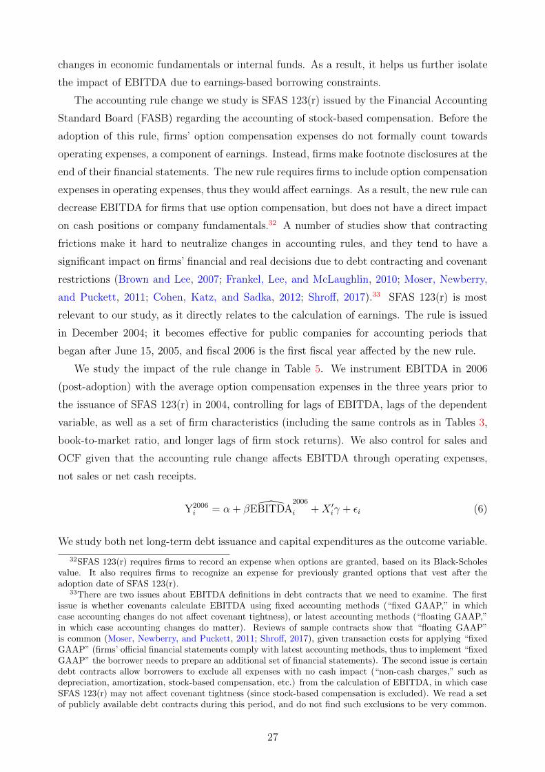
changes in economic fundamentals or internal funds. As a result, it helps us further isolate
the impact of EBITDA due to earnings-based borrowing constraints.
The accounting rule change we study is SFAS 123(r) issued by the Financial Accounting
Standard Board (FASB) regarding the accounting of stock-based compensation. Before the
adoption of this rule, firms’ option compensation expenses do not formally count towards
operating expenses, a component of earnings. Instead, firms make footnote disclosures at the
end of their financial statements. The new rule requires firms to include option compensation
expenses in operating expenses, thus they would affect earnings. As a result, the new rule can
decrease EBITDA for firms that use option compensation, but does not have a direct impact
on cash positions or company fundamentals.32 A number of studies show that contracting
frictions make it hard to neutralize changes in accounting rules, and they tend to have a
significant impact on firms’ financial and real decisions due to debt contracting and covenant
restrictions (Brown and Lee, 2007; Frankel, Lee, and McLaughlin, 2010; Moser, Newberry,
and Puckett, 2011; Cohen, Katz, and Sadka, 2012; Shroff, 2017).33 SFAS 123(r) is most
relevant to our study, as it directly relates to the calculation of earnings. The rule is issued
in December 2004; it becomes effective for public companies for accounting periods that
began after June 15, 2005, and fiscal 2006 is the first fiscal year affected by the new rule.
We study the impact of the rule change in Table 5. We instrument EBITDA in 2006
(post-adoption) with the average option compensation expenses in the three years prior to
the issuance of SFAS 123(r) in 2004, controlling for lags of EBITDA, lags of the dependent
variable, as well as a set of firm characteristics (including the same controls as in Tables 3,
book-to-market ratio, and longer lags of firm stock returns). We also control for sales and
OCF given that the accounting rule change affects EBITDA through operating expenses,
not sales or net cash receipts.
Y2006i = α + β EBITDA
2006
i +X ′iγ + εi (6)
We study both net long-term debt issuance and capital expenditures as the outcome variable.
32SFAS 123(r) requires firms to record an expense when options are granted, based on its Black-Scholesvalue. It also requires firms to recognize an expense for previously granted options that vest after theadoption date of SFAS 123(r).
33There are two issues about EBITDA definitions in debt contracts that we need to examine. The firstissue is whether covenants calculate EBITDA using fixed accounting methods (“fixed GAAP,” in whichcase accounting changes do not affect covenant tightness), or latest accounting methods (“floating GAAP,”in which case accounting changes do matter). Reviews of sample contracts show that “floating GAAP”is common (Moser, Newberry, and Puckett, 2011; Shroff, 2017), given transaction costs for applying “fixedGAAP” (firms’ official financial statements comply with latest accounting methods, thus to implement “fixedGAAP” the borrower needs to prepare an additional set of financial statements). The second issue is certaindebt contracts allow borrowers to exclude all expenses with no cash impact (“non-cash charges,” such asdepreciation, amortization, stock-based compensation, etc.) from the calculation of EBITDA, in which caseSFAS 123(r) may not affect covenant tightness (since stock-based compensation is excluded). We read a setof publicly available debt contracts during this period, and do not find such exclusions to be very common.
27
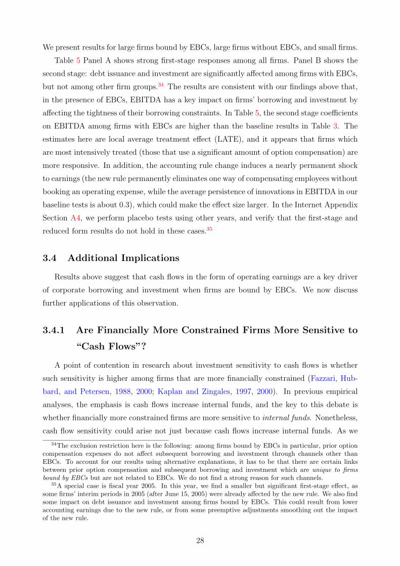
We present results for large firms bound by EBCs, large firms without EBCs, and small firms.
Table 5 Panel A shows strong first-stage responses among all firms. Panel B shows the
second stage: debt issuance and investment are significantly affected among firms with EBCs,
but not among other firm groups.34 The results are consistent with our findings above that,
in the presence of EBCs, EBITDA has a key impact on firms’ borrowing and investment by
affecting the tightness of their borrowing constraints. In Table 5, the second stage coefficients
on EBITDA among firms with EBCs are higher than the baseline results in Table 3. The
estimates here are local average treatment effect (LATE), and it appears that firms which
are most intensively treated (those that use a significant amount of option compensation) are
more responsive. In addition, the accounting rule change induces a nearly permanent shock
to earnings (the new rule permanently eliminates one way of compensating employees without
booking an operating expense, while the average persistence of innovations in EBITDA in our
baseline tests is about 0.3), which could make the effect size larger. In the Internet Appendix
Section A4, we perform placebo tests using other years, and verify that the first-stage and
reduced form results do not hold in these cases.35
3.4 Additional Implications
Results above suggest that cash flows in the form of operating earnings are a key driver
of corporate borrowing and investment when firms are bound by EBCs. We now discuss
further applications of this observation.
3.4.1 Are Financially More Constrained Firms More Sensitive to
“Cash Flows”?
A point of contention in research about investment sensitivity to cash flows is whether
such sensitivity is higher among firms that are more financially constrained (Fazzari, Hub-
bard, and Petersen, 1988, 2000; Kaplan and Zingales, 1997, 2000). In previous empirical
analyses, the emphasis is cash flows increase internal funds, and the key to this debate is
whether financially more constrained firms are more sensitive to internal funds. Nonetheless,
cash flow sensitivity could arise not just because cash flows increase internal funds. As we
34The exclusion restriction here is the following: among firms bound by EBCs in particular, prior optioncompensation expenses do not affect subsequent borrowing and investment through channels other thanEBCs. To account for our results using alternative explanations, it has to be that there are certain linksbetween prior option compensation and subsequent borrowing and investment which are unique to firmsbound by EBCs but are not related to EBCs. We do not find a strong reason for such channels.
35A special case is fiscal year 2005. In this year, we find a smaller but significant first-stage effect, assome firms’ interim periods in 2005 (after June 15, 2005) were already affected by the new rule. We also findsome impact on debt issuance and investment among firms bound by EBCs. This could result from loweraccounting earnings due to the new rule, or from some preemptive adjustments smoothing out the impactof the new rule.
28
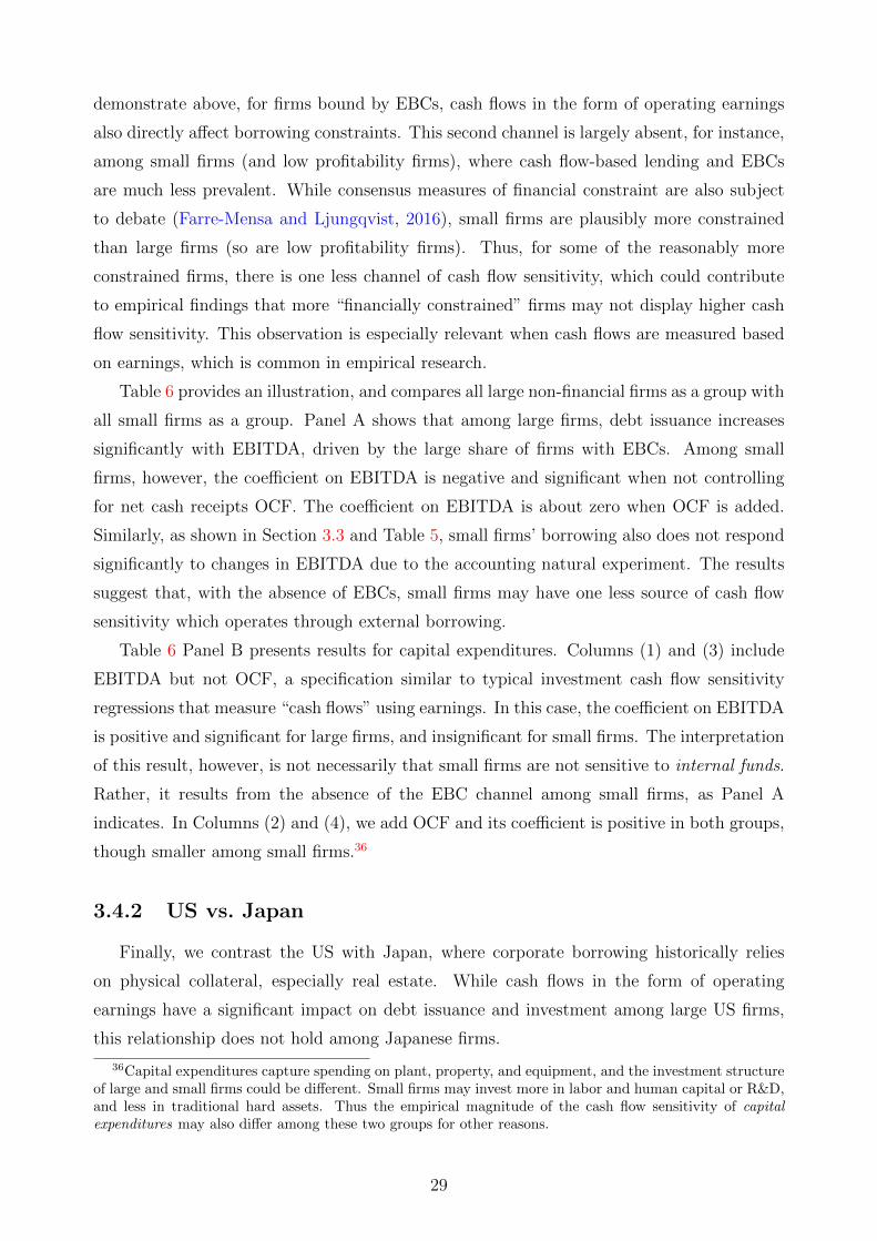
demonstrate above, for firms bound by EBCs, cash flows in the form of operating earnings
also directly affect borrowing constraints. This second channel is largely absent, for instance,
among small firms (and low profitability firms), where cash flow-based lending and EBCs
are much less prevalent. While consensus measures of financial constraint are also subject
to debate (Farre-Mensa and Ljungqvist, 2016), small firms are plausibly more constrained
than large firms (so are low profitability firms). Thus, for some of the reasonably more
constrained firms, there is one less channel of cash flow sensitivity, which could contribute
to empirical findings that more “financially constrained” firms may not display higher cash
flow sensitivity. This observation is especially relevant when cash flows are measured based
on earnings, which is common in empirical research.
Table 6 provides an illustration, and compares all large non-financial firms as a group with
all small firms as a group. Panel A shows that among large firms, debt issuance increases
significantly with EBITDA, driven by the large share of firms with EBCs. Among small
firms, however, the coefficient on EBITDA is negative and significant when not controlling
for net cash receipts OCF. The coefficient on EBITDA is about zero when OCF is added.
Similarly, as shown in Section 3.3 and Table 5, small firms’ borrowing also does not respond
significantly to changes in EBITDA due to the accounting natural experiment. The results
suggest that, with the absence of EBCs, small firms may have one less source of cash flow
sensitivity which operates through external borrowing.
Table 6 Panel B presents results for capital expenditures. Columns (1) and (3) include
EBITDA but not OCF, a specification similar to typical investment cash flow sensitivity
regressions that measure “cash flows” using earnings. In this case, the coefficient on EBITDA
is positive and significant for large firms, and insignificant for small firms. The interpretation
of this result, however, is not necessarily that small firms are not sensitive to internal funds.
Rather, it results from the absence of the EBC channel among small firms, as Panel A
indicates. In Columns (2) and (4), we add OCF and its coefficient is positive in both groups,
though smaller among small firms.36
3.4.2 US vs. Japan
Finally, we contrast the US with Japan, where corporate borrowing historically relies
on physical collateral, especially real estate. While cash flows in the form of operating
earnings have a significant impact on debt issuance and investment among large US firms,
this relationship does not hold among Japanese firms.
36Capital expenditures capture spending on plant, property, and equipment, and the investment structureof large and small firms could be different. Small firms may invest more in labor and human capital or R&D,and less in traditional hard assets. Thus the empirical magnitude of the cash flow sensitivity of capitalexpenditures may also differ among these two groups for other reasons.
29

Table 7 reruns the baseline regressions among large non-financial firms (i.e. assets above
median among public firms in the respective country) in the US and Japan. A majority of
firms in the US large firm sample have EBCs, as shown in Section 2.1.2, while cash flow-based
lending and EBCs are less common in Japan (Tan, 2004). Table 7 Panel A first tabulates
the summary statistics for the US and Japan samples. For Japanese firms, we use data from
Compustat Global, supplemented with stock price information from Datastream. Net long-
term debt issuance from the statement of cash flows is not available for the Japan sample,
so we measure debt issuance here using changes in total book debt. Capital expenditures
and net cash receipts (OCF) are also available for a smaller set of Japan firms before 2000,
and we fill in the gap using additional data from WorldScope. Firms in the US and Japan
samples are similar in size as measured by assets. US firms have higher EBITDA relative to
assets, as well as higher equity valuations. US firms have higher debt relative to assets, and
Japanese firms have higher debt relative to EBITDA (as Japanese firms are not bound by
debt to EBITDA constraints).
Table 7 Panel B performs the baseline regressions in the US and Japan samples. There is
a strong positive relationship between debt issuance and EBITDA in the US sample (driven
by firms bound by EBCs), which is absent in the Japan sample. As shown by Panel B column
(3), in the Japan sample, debt issuance decreases with EBITDA in when not controlling for
net cash receipts OCF. Once we control for OCF in column (4), the EBITDA coefficient
becomes close to zero and OCF has a significantly negative coefficient. Similarly, EBITDA
does not have an independent impact on investment in the Japan sample.
Borrowing Constraints and Cash Flow Value. Results in this section suggest
that, with cash flow-based lending and EBCs, cash flows in the form of operating earnings
(EBITDA) relax borrowing constraints and help firms borrow and invest more. These ef-
fects are not present, however, when asset-based lending prevails. Given contracting frictions
discussed in Section 2.1.2, current EBITDA is central to commonly used, legally binding bor-
rowing constraints (EBCs), and exhibits a disproportionate impact. While current EBITDA
is an important factor and an anchor of EBCs, other factors such as expected present value
of future cash flows may also play a role. For instance, a firm with high future cash flow
prospects could be able to get a larger loan relative to its current EBITDA, and a higher
debt to EBITDA multiple for its covenant constraints. We focus on the effect of current
EBITDA as an illustration of the central role of cash flow value in corporate borrowing in
the US, both because it has a disproportionate impact due to contracting frictions, and be-
cause it is directly observable in the data (the present value of future cash flows, on the other
hand, is hard to empirically measure; it is also empirically hardly separable from investment
opportunities).
30

After investigating how corporate borrowing practices shape the role of cash flows, in the
next section we examine how they affect the role of physical assets to provide a fuller picture
and lay out additional implications.
4 Property Prices, Firm Outcomes, and Financial Ac-
celeration
In this section, we study how corporate borrowing practices also help understand firms’
sensitivity to collateral value, specifically property prices, and illuminate the transmission of
shocks during the Great Recession.
We first examine the general sensitivity of US firms’ borrowing to property collateral
value. We find that borrowing increases by about three cents for a one dollar increase in
the value of real estate assets, consistent with prior research (Chaney, Sraer, and Thesmar,
2012; Cvijanovic, 2014). Moreover, this positive sensitivity is concentrated in asset-based
debt; it is absent (if not negative) among cash flow-based debt. Thus the overall sensitivity
to real estate value appears modest. The magnitude is smaller than the average sensitivity
of debt issuance to operating earnings among US large non-financial firms (about 20 cents).
The magnitude also suggests that a 20% property price drop would have a limited impact
on the median firm with real estate holdings.
We then use this observation to shed further light on the transmission of property price
declines during the Great Recession. Since the Great Recession, a vibrant literature led
by Mian and Sufi (2014) studies the transmission of the property price collapse through
household balance sheets and household demand. Much less attention is paid to firms,
who in principle are also owners of real estate capital and may suffer similar collateral
damage. Indeed, collateral damage to firms plays a critical role both in theories of financial
acceleration and in some international experiences. In textbook macro-finance models, firms’
debt capacity is driven by the liquidation value of physical capital, and financial acceleration
operates through fire-sale amplifications: a drop in the liquidation value of physical assets
tightens borrowing constraints, squeezes firms’ ability to hold capital, further compresses
the price of assets, and triggers an asset price feedback loop (Kiyotaki and Moore, 1997;
Bernanke, Gertler, and Gilchrist, 1999). Firms’ collateral damage also appears central in the
Japanese crisis in the early 1990s. Figure 5 shows that Japanese corporate debt experienced
a sizable boom-bust cycle together with real estate value (Panel A). In sharp contrast, during
the US property price cycle in the 2000s, corporate debt only budged relative to property
prices and household debt (Panel B).
We tie these threads together by examining how collateral damage due to property price
31
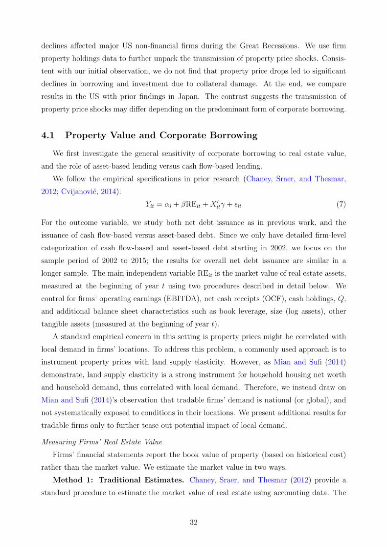
declines affected major US non-financial firms during the Great Recessions. We use firm
property holdings data to further unpack the transmission of property price shocks. Consis-
tent with our initial observation, we do not find that property price drops led to significant
declines in borrowing and investment due to collateral damage. At the end, we compare
results in the US with prior findings in Japan. The contrast suggests the transmission of
property price shocks may differ depending on the predominant form of corporate borrowing.
4.1 Property Value and Corporate Borrowing
We first investigate the general sensitivity of corporate borrowing to real estate value,
and the role of asset-based lending versus cash flow-based lending.
We follow the empirical specifications in prior research (Chaney, Sraer, and Thesmar,
2012; Cvijanovic, 2014):
Yit = αi + βREit +X ′itγ + εit (7)
For the outcome variable, we study both net debt issuance as in previous work, and the
issuance of cash flow-based versus asset-based debt. Since we only have detailed firm-level
categorization of cash flow-based and asset-based debt starting in 2002, we focus on the
sample period of 2002 to 2015; the results for overall net debt issuance are similar in a
longer sample. The main independent variable REit is the market value of real estate assets,
measured at the beginning of year t using two procedures described in detail below. We
control for firms’ operating earnings (EBITDA), net cash receipts (OCF), cash holdings, Q,
and additional balance sheet characteristics such as book leverage, size (log assets), other
tangible assets (measured at the beginning of year t).
A standard empirical concern in this setting is property prices might be correlated with
local demand in firms’ locations. To address this problem, a commonly used approach is to
instrument property prices with land supply elasticity. However, as Mian and Sufi (2014)
demonstrate, land supply elasticity is a strong instrument for household housing net worth
and household demand, thus correlated with local demand. Therefore, we instead draw on
Mian and Sufi (2014)’s observation that tradable firms’ demand is national (or global), and
not systematically exposed to conditions in their locations. We present additional results for
tradable firms only to further tease out potential impact of local demand.
Measuring Firms’ Real Estate Value
Firms’ financial statements report the book value of property (based on historical cost)
rather than the market value. We estimate the market value in two ways.
Method 1: Traditional Estimates. Chaney, Sraer, and Thesmar (2012) provide a
standard procedure to estimate the market value of real estate using accounting data. The
32

estimate is calculated based on the book value of real estate, accumulated depreciation,
and historical property value in the firm’s headquarters location. Because accumulated
depreciation on real estate assets is no longer reported after 1993, this procedure requires
firms to be public since 1993, which restricts the sample size. The key assumption in this
estimate is that most of the real estate firms own are located near their headquarters, which
is plausible as we discuss in more detail below (most firms’ owned properties, such as offices
and main production facilities, tend to concentrate in the headquarters region). Appendix
G explains the construction of our estimates by step.
Table 8 presents the characteristics of this sample. Given the data requirement of this
method, the sample tilts towards large firms (70%). 56% of the sample have earnings-based
covenants. Median market value of real estate normalized by book assets is 0.20; median
market value of real estate relative to the market value of equity 0.20, very similar to Chaney,
Sraer, and Thesmar (2012). Table 8 also shows the characteristics of all public firms that
own real estate (around 66% of Compustat own some real estate), measured during the same
period. In comparison, firms in the Method 1 sample are slightly larger in size, but generally
similar in terms of the amount of book PPE, profitability and book leverage.
Method 2: Property Ownership Information from Annual Reports. US non-
financial firms are required to discuss their physical properties in annual reports. About one
third of firms with real estate provide a detailed list of their owned properties, including
location, property type, and square footage. We hand collect these data from 2006 filings
to get more refined information about firms’ property holdings. For the panel analysis in
this section, we assume firms own a fixed set of properties as shown by 2006 filings, estimate
the market value of each property in each year, and sum up to the firm level. Our baseline
results use property locations in 2006 filings to align with the cross-sectional analysis in
Section 4.2 (we also read filings in 2002, which produce similar results; estimates using
locations in 2002 and 2006 filings are about 0.85 correlated). For the cross-sectional analysis
in Section 4.2 focusing on the crisis period, we directly take the properties owned by the
end of 2006 reported in the 2006 filings, and calculate their values through the crisis. We
restrict to owned real estate located in the US, and keep firms that have information for
substantially all owned properties in the US. Appendix G provides examples of property
holding information from 10-K filings, and detailed explanations of variable construction.
The market value of real estate measured using Method 1 and Method 2 is consistent.
For firms in both samples, the estimates are 0.7 correlated. The levels also match up. The
similarity is high because most firms’ owned properties are limited and are concentrated in the
headquarters location, so the assumption used in traditional estimates largely holds (e.g. as
of 2006 Starbucks only owns some headquarters office space and four roasting facilities).
Table 8 also reports the characteristics of firms in the Method 2 sample. These firms
33

are slightly smaller than those in the Method 1 sample (60% of the sample are large firms).
They utilize more asset-based lending compared to the Method 1 sample, although cash
flow-based lending still accounts for the majority of their debt (median share is 65%); 47%
have earnings-based covenants. They are similar to other firms with real estate in terms of
book PPE and profitability, and have slightly lower book leverage.
Results
Table 9 presents the results, for all firms where real estate value measures are available as
well as the subsample consisting of tradable firms only. We get similar results across different
samples. A one dollar increase in real estate value is on average associated with an increase
in net long-term debt issuance of about three cents. The positive response is concentrated in
asset-based debt. It is absent among cash flow-based debt. We can further break down cash
flow-based debt into cash flow-based loans and bonds, and the positive sensitivity is absent
in both categories. These patterns hold not just for debt issuance, but also for the level of
debt, as shown in Appendix B Table A3.
Results in Table 9 are similar whether we restrict to tradable firms or not. Public non-
financial firms in our samples are generally sufficiently large that their product demand may
not be concentrated in areas where they own properties, even for some of the non-tradable
firms (e.g. Starbucks is categorized as a non-tradable firm, but it owns primarily roasting
facilities that are far from its product markets; however, caveats may apply to services firms
that are real estate heavy and have few locations, like casinos and amusement parks, where
property location and product market overlap). For most firms, property price shocks at
firms’ real estate locations seem sufficiently exogenous to their product demand.
In Table 9 the coefficients on EBITDA are significant, and the magnitudes are compara-
ble with our findings in Section 3 (the EBITDA coefficients in Table 9 are about 0.15 to 0.2,
driven by the roughly 60% of firms in these samples with EBCs). In our samples which pri-
marily consist of large firms that borrow through cash flow-based lending, EBITDA appears
to have a bigger average impact on borrowing than property collateral value (0.03).
Taken together, the results suggest that a substantial portion of large non-financial firms’
debt does not rely significantly on real estate value. With these alternative venues for
borrowing, the overall sensitivity to property prices appears limited. For instance, for a firm
with a median level of real estate holdings (real estate value is 0.2 times book asset value),
a 20% decline in property price would decrease its real estate value by about 4% of book
asset value, and reduce its borrowing by about 0.1 basis points (4%×0.03). This effect is
small relative to a median investment rate (CAPX normalized by assets) of 5 basis points
(0.05) and a median EBITDA to assets ratio of 13 basis points (0.13) among large firms. In
the following, we use this observation to shed light on features of the Great Recession, and
34

further unpack the transmission of property price declines.
4.2 The Great Recession: Unpacking the Property Price Effect
Since the Great Recession, a vibrant strand of research investigates the impact of the
property value collapse. The key insight is that property price declines damaged household
balance sheets, dried up aggregate demand, and led to drops in investment and employment
(Mian and Sufi, 2014; Giroud and Mueller, 2017). Property price declines, however, may also
transmit through collateral damage to firms. Less is known about the role of this second
channel in the Great Recession. Such a mechanism could be powerful if firms’ debt capacity
relies heavily on property collateral value; it could be attenuated if firms primarily utilize
cash flow-based lending.
In the following, we examine the impact of corporate property value in the Great Reces-
sion. We proceed in two steps. We first note that the limited impact due to declines in firms’
property value could be inferred from insights in the household demand channel. Specifically,
Mian and Sufi (2014) study the impact of property prices on local employment growth during
the Great Recession, and propose a comparison of tradable versus non-tradable industries.
The key idea is that property prices affect local household demand: firms in non-tradable in-
dustries are exposed to local demand, so they should be more sensitive to local property price
changes. Firms in tradable industries, on the other hand, face demand from a larger market,
so they should be less sensitive. Consistent with the hypothesis, Mian and Sufi (2014) find
strong responses of local employment to local house prices among non-tradable firms. They
do not find any relationship among tradable firms. Giroud and Mueller (2017) find similar
strong relationships among non-tradable firms, and no relationship among tradable firms.
Nonetheless, property price declines at a firm’s location affect not only local demand,
but also the value of the firm’s real estate assets. This channel through property collateral
value is relevant for both tradable and non-tradable firms. If this channel is strong, we would
expect that tradable firms also display some sensitivity to local property price changes. The
null result from prior work thus hints at the muted impact of property collateral damage
among US non-financial firms in the Great Recession.
We then further unpack the transmission of property price declines in the Great Reces-
sion in Table 10. We disentangle the firm-side property collateral value channel using firm
property holdings data. We exploit firms’ differential exposures to property value shocks
through the following cross-sectional specification:
∆Y 07−09i = α + λ∆RE07−09
i + ηRE06i + φ∆P 07−09
i + β∆EBITDA07−09i +X ′iγ + ui (8)
35

The left hand side variable Y 07−09i is outcomes of firm i from 2007 to 2009. In Panel A,
∆Y 07−09i is the change in net long-term debt issuance from 2007 to 2009. In Panel B,
∆Y 07−09i is the change in capital expenditures. On the right hand side, the key variable of
interest is ∆RE07−09i,06 , which captures changes in firm i’s real estate value from 2007 to 2009.
It is measured as the market value gain/loss of firm i’s pre-crisis (end of 2006) real estate
holdings during the Great Recession, normalized by assets in 2006. This variable is the main
focus for analyzing the property collateral channel. We also include RE06i , which controls
for firm i’s pre-crisis real estate holdings (normalized by assets in 2006). In addition, we
control for ∆P 07−09i , the percentage change in property prices in firm i’s locations, which
captures the impact of property prices that may work through local household demand. We
also control for changes in EBITDA, net cash receipts, and Q from 2007 to 2009, as well as
Q, leverage, cash holdings, size (log assets) by the end of 2006, among others.
We measure firms’ real estate value using both of the methods described in the previous
section. For Method 1, we calculate firm-level RE06i , ∆RE07−09
i,06 , and ∆P 07−09i all using head-
quarters information. Specifically, RE06i is constructed based on the regular headquarters-
based procedure, ∆P 07−09i is the percent change in property prices in the headquarters lo-
cation from 2007 to 2009, and ∆RE07−09i,06 = RE06
i × ∆P 07−09i . For Method 2, we calculate
firm-level RE06i , ∆RE07−09
i,06 , and ∆P 07−09i by aggregating information from each owned prop-
erty j of firm i. Specifically, we then sum across these properties to obtain RE06i =
∑j RE06
i,j
and ∆RE07−09i,06 =
∑j RE06
i,j ×∆P 07−09i,j , where ∆P 07−09
i,j is the percentage change in property
prices in the location of owned property j of firm i. In this case, we calculate ∆P 07−09i as
the average of ∆P 07−09i,j ; we can alternatively calculate firm-level ∆P 07−09
i using property
price changes in firm i’s headquarters or average across all locations (owned and leased), and
the results are similar. The bottom of Table 8 shows additional summary statistics during
the crisis. For firms in our sample, the median property price decline from 2007 to 2009,
∆P 07−09i , is about 8%. The median decline in the market value of real estate assets from
2007 to 2009 (normalized by 2006 assets), ∆RE07−09i,06 , is about 0.01.
In this setting, there could still be concerns about property prices being correlated with
local demand. In our current cross-sectional set-up, this issue can drive down λ if firms
that own more real estate are systematically less sensitive to local demand. As discussed
in Section 4.1, the local demand issue does not appear severe for large public firms whose
demand is generally not local. Nonetheless, we also perform additional checks in Internet
Appendix Table IA7 using tradable firms only.
Table 10 presents results using different estimates. We tease out the outliers and make
sure they do not drive our results. We also report both OLS estimates and least absolute
deviation (LAD) estimates (following Gan (2007)) to further alleviate the influence of outliers
and skewness in the cross-sectional data. Across different estimates, we do not find evidence
36

that declines in firms’ real estate value drove down debt issuance or capital expenditures
during the Great Recession. The lack of significant results could be in part because the
sensitivity is very small (as discussed in Section 4.1), which makes it hard to detect in
a regular cross section. It could also be related to the structure of loans backed by real
estate, where loan-to-value constraints affect issuance but do not always affect maintenance
of existing loans.37 Finally, in Table 10 the coefficients on EBITDA and OCF have the same
signs and comparable magnitudes as results in Section 3.
In summary, our analysis suggests that property price declines during the Great Recession
did not have a significant impact on firms’ outcomes due to collateral damage. In the
following, we compare and contrast results from the US housing collapse with previous
research on Japan’s housing collapse. We highlight substantial differences in the transmission
of property price shocks under different regimes of corporate lending.
4.3 Property Price Declines and the Firm Collateral Channel: US
and Japan
In the late 1980s and early 1990s, Japan experienced a major boom-bust cycle in property
prices. The collapse of property prices had a far-reaching impact on Japan’s economy. As
discussed earlier, corporate borrowing in Japan traditionally relies on real estate collateral,
especially before the bankruptcy reforms in the early 2000s. Thus Japan’s real estate collapse
took place in an environment where property value is central for corporate credit.
With the collapse of property prices, Japanese firms’ debt capacity and investment ac-
tivities suffered significantly, as documented by Gan (2007). Gan (2007) studies public
manufacturing firms in Japan, and uses the value of firms’ real estate prior to the collapse as
the main measure of exposures to property price shocks (she estimates the market value of
real estate from accounting data through a procedure similar to method 1 above). She finds
that Japanese firms that owned more property pre-collapse suffered particularly severely dur-
ing the bust: for a one dollar increase in a firm’s pre-collapse land holdings in 1989, average
CAPX investment is lower by 13 to 16 cents from 1994 to 1998. The impact is substantial,
especially that property prices peaked around 1990, and the outcome is measured as the
average over five years after 1994.
In Table 11, we present results in the US sample using the same regression specifications
37Accordingly, when property value increases, a firm can take out a larger loan based on a given loanto property value ratio that is evaluated at issuance. When the property value declines, however, the firmwould not be forced to shrink the size of existing loans. The option to take out larger loans when propertyprices increase, coupled with the lack of forced debt reduction when property prices drop, could contributeto less sensitivity to property value in recessions than in normal times.
37

as Table 2 column (2) of Gan (2007):
CAPXposti = α + βREpre
i +X ′iγ + vi (9)
where CAPXposti is firm i’s average annual investment rate over a period of time during
the property price collapse; REprei is the value of firm i’s real estate holdings prior to the
collapse, which captures firms’ exposures to real estate; Xi includes firm level controls (cash
flows during the post period, Q, cash holdings, a dummy indicating firms with above median
real estate holdings, and interactions of cash flows and cash holdings with this dummy). This
specification is different from our tests in Equation (8) above and provides an alternative
test. As Table 11 shows, in the US Great Recession, we do not find results similar to
what Gan (2007) found in Japan. There is no significant correlation between a firms’ pre-
crisis real estate holdings and its subsequent outcome. The sharp contrast suggests that the
transmission mechanisms of a property price collapse could be different in different settings,
depending on the lending regime and the central determinants of firms’ debt capacity.
4.4 Earnings Drop and Firm Outcomes in the Great Recession
Finally, we perform a simple assessment of the impact of earnings-based borrowing con-
straints during the Great Recession.
In our data, total earnings of large public firms with EBCs fell by $123 billion from 2007
to 2009. Based on baseline results in Table 3, this is associated with a $33.5 billion decline in
long-term net debt issuance due to EBCs, which accounts for 10.6% of the issuance decline
among all public firms. It is associated with a $14 billion reduction in CAPX due to EBCs,
which accounts for 8.7% of CAPX declines among public firms. If we augment the baseline
regression with two dummy variables indicating covenant violation and within 0.5 standard
deviations of violation to allow for discontinuity in outcome variables due to violations, the
total impact increases slightly to 14.4% of declines in net long-term debt issuance and 9.5%
of declines in CAPX. Finally, if we instead estimate a cross-sectional regression for firms
with EBCs focusing on the Great Recession period, results are similar (EBCs account for
10.7% of declines in net long-term debt issuance and 9% of declines in CAPX).38
38For Estimate 1, we use the regression in Table 3, and calculate the change in the outcome variablepredicted by the change in EBITDA. We renormalize the outcome to dollar amounts and sum across alllarge firms with EBCs. For Estimate 2, the procedure is the same, except we add two dummies to capturepotential non-linear impact when firms violate earnings-based covenants or are very close to violation. ForEstimate 3, we instead use cross-sectional regressions restricted to the Great Recession period. We run across-sectional regression among large non-financial firms with EBCs: ∆Y 07−09
i = α + β∆EBITDA07−09i +
κ∆OCF07−09i + X ′iγ + ui, where ∆Y 07−09
i is firm i’s change in net debt issuance (or CAPX) from 2007 to2009, ∆EBITDA07−09
i is its change in EBITDA; controls include changes in Q and pre-crisis Q, as well ascash holdings, book leverage, book PPE, size, among other firm characteristics measured at the end of 2006.We then calculate changes in the outcome variable predicted by changes in EBITDA. Finally, we sum up
38

Overall, the estimated impact due to EBCs is meaningful but not catastrophic. Combined
with previous results on the limited impact of property collateral value, one may speculate
that the US has developed a relatively resilient corporate borrowing system among large
non-financial firms. With cash flow-based lending and EBCs, firms could be less exposed
to fire sale amplifications studied in textbook macro-finance models. The balance sheets
of firms alone may not be the key financial accelerator. In comparison, the impairment of
banks’ balance sheets (Chodorow-Reich, 2014; Becker and Ivashina, 2014; Chodorow-Reich
and Falato, 2017) and household demand (Mian and Sufi, 2014) can be the primary sources
of vulnerability in the US setting.
5 Conclusion
In this paper, we study borrowing constraints of non-financial firms. We show that
cash flow-based lending accounts for the vast majority of large US non-financial firms’ debt.
With cash flow-based lending, a standard borrowing constraint restraint restricts a firm’s
total debt based on a particular measure of cash flows, namely operating earnings. We lay
out determinants of these borrowing practices, and delineate differences in the predominant
form of corporate borrowing across firm groups.
Understanding how firms borrow helps tie together several issues. The prevalence of
cash flow-based lending and EBCs shapes the way cash flows affect corporate borrowing. In
particular, cash flows in the form of operating earnings relax EBCs, and play a key role in
facilitating borrowing. This mechanism further suggests a new channel for the sensitivity
of firms’ investment to cash flows which operates through external borrowing. Among firms
that rely on asset-based lending due to a variety of reasons, these patterns are absent, which
helps account for variations in firm behavior. The prevalence of cash flow-based lending
also alleviates firms’ dependence on the value of physical assets. Correspondingly, large US
firms’ borrowing and investment were not particularly vulnerable to property price declines
in the Great Recession through collateral damage. The results suggest that corporate balance
sheets may not be the central amplifier of financial shocks in the US setting, and shed light
on why the Great Recession is a crisis centered around households and banks rather than
major non-financial firms.
Our study analyzes non-financial firms. A question for future work is to investigate the
form of borrowing constraints among various types of financial institutions, how they differ,
why, and the corresponding implications.
the firm level impact across all large non-financial firms with EBCs.
39

References
Acharya, Viral V, Heitor Almeida, Filippo Ippolito, and Ander Perez-Orive, 2014, Bank linesof credit as contingent liquidity: A study of covenant violations and their implications,Working paper.
Adelino, Manuel, Antoinette Schoar, and Felipe Severino, 2015, House prices, collateral, andself-employment, Journal of Financial Economics 117, 288–306.
Aghion, Philippe, and Patrick Bolton, 1992, An incomplete contracts approach to financialcontracting, Review of Economic Studies 59, 473–494.
Almeida, Heitor, and Murillo Campello, 2007, Financial constraints, asset tangibility, andcorporate investment, Review of Financial Studies 20, 1429–1460.
Almeida, Heitor, Murillo Campello, and Michael S Weisbach, 2004, The cash flow sensitivityof cash, Journal of Finance 59, 1777–1804.
Baker, Malcolm, Jeremy C Stein, and Jeffrey Wurgler, 2003, When does the market matter?Stock prices and the investment of equity-dependent firms, Quarterly Journal of Economics118, 969–1005.
Barro, Robert J, 1990, The stock market and investment, Review of Financial Studies 3,115–131.
Becker, Bo, and Victoria Ivashina, 2014, Cyclicality of credit supply: Firm level evidence,Journal of Monetary Economics 62, 76–93.
Becker, Bo, and Victoria Ivashina, 2016, Covenant-light contracts and creditor coordination,Working paper.
Benmelech, Efraim, and Nittai K Bergman, 2009, Collateral pricing, Journal of FinancialEconomics 91, 339–360.
Benmelech, Efraim, and Nittai K Bergman, 2011, Bankruptcy and the collateral channel,Journal of Finance 66, 337–378.
Bernanke, Ben S, Mark Gertler, and Simon Gilchrist, 1999, The financial accelerator in aquantitative business cycle framework, Handbook of Macroeconomics 1, 1341–1393.
Bernstein, Shai, Emanuele Colonnelli, and Ben Iverson, 2017, Asset allocation in bankruptcy,Working paper.
Bhattacharya, Utpal, Hazem Daouk, and Michael Welker, 2003, The world price of earningsopacity, Accounting Review 78, 641–678.
Blanchard, Olivier Jean, Florencio Lopez-de Silanes, and Andrei Shleifer, 1994, What dofirms do with cash windfalls?, Journal of Financial Economics 36, 337–360.
Bradley, Michael, and Michael R Roberts, 2015, The structure and pricing of corporate debtcovenants, Quarterly Journal of Finance 5, 1550001.
Bris, Arturo, Ivo Welch, and Ning Zhu, 2006, The costs of bankruptcy: Chapter 7 liquidationversus Chapter 11 reorganization, Journal of Finance 61, 1253–1303.
Brown, Lawrence D, and Yen-Jung Lee, 2007, The determinants and consequences of changesin executive option-based compensation around the issuance of SFAS 123r, Working paper.
Brunnermeier, Markus K, and Yuliy Sannikov, 2014, A macroeconomic model with a financialsector, American Economic Review 104, 379–421.
40

Catherine, Sylvain, Thomas Chaney, Zongbo Huang, David A Sraer, and David Thesmar,2017, Aggregate effects of collateral constraints, Working paper.
Chaney, Thomas, David Sraer, and David Thesmar, 2012, The collateral channel: How realestate shocks affect corporate investment, American Economic Review 102, 2381–2409.
Chava, Sudheer, and Michael R Roberts, 2008, How does financing impact investment? Therole of debt covenants, Journal of Finance 63, 2085–2121.
Chodorow-Reich, Gabriel, 2014, The employment effects of credit market disruptions: Firm-level evidence from the 2008–9 financial crisis, Quarterly Journal of Economics 129, 1–59.
Chodorow-Reich, Gabriel, and Antonio Falato, 2017, The loan covenant channel: How bankhealth transmits to the real economy, Working paper.
Cohen, Moshe, Sharon P Katz, and Gil Sadka, 2012, Debt covenants and capital structure:Evidence from an exogenous shock to debt capacity, Working paper.
Coval, Joshua, and Erik Stafford, 2007, Asset fore sales and (purchases) in equity markets,Journal of Financial Economics 86, 479–512.
Cvijanovic, Dragana, 2014, Real estate prices and firm capital structure, Review of FinancialStudies 27, 2690–2735.
Dechow, Patricia M, and Ilia D Dichev, 2002, The quality of accruals and earnings: The roleof accrual estimation errors, Accounting Review 77, 35–59.
Demerjian, Peter R, 2011, Accounting standards and debt covenants: Has the “balance sheetapproach” led to a decline in the use of balance sheet covenants?, Journal of Accountingand Economics 52, 178–202.
Demerjian, Peter R, and Edward L Owens, 2016, Measuring the probability of financialcovenant violation in private debt contracts, Journal of Accounting and Economics 61,433–447.
Demirci, Irem, Umit G Gurun, and Erkan Yonder, 2017, Shuffling through the bargain bin:Real estate holdings of public firms, Working paper.
Denis, David J, and Stephen B McKeon, 2016, Persistent operating losses and corporatefinancial policies, Working paper.
Diamond, Douglas W, Yunzhi Hu, and Raghuram G Rajan, 2017, Pledgeability, industryliquidity, and financing cycles, Working paper.
Djankov, Simeon, Oliver Hart, Caralee McLiesh, and Andrei Shleifer, 2008, Debt enforcementaround the world, Journal of Political Economy 116, 1105–1149.
Falato, Antonio, and Nellie Liang, 2016, Do creditor rights increase employment risk? Evi-dence from loan covenants, Journal of Finance 71, 2545–2590.
Farre-Mensa, Joan, and Alexander Ljungqvist, 2016, Do measures of financial constraintsmeasure financial constraints?, Review of Financial Studies 29, 271–308.
Fazzari, Steven M, R Glenn Hubbard, and Bruce C Petersen, 1988, Financing constraintsand corporate investment, Brookings Papers on Economic Activity 1988, 141–206.
Fazzari, Steven M, R Glenn Hubbard, and Bruce C Petersen, 2000, Investment-cash flow sen-sitivities are useful: A comment on Kaplan and Zingales, Quarterly Journal of Economics115, 695–705.
Francis, Jennifer, Ryan LaFond, Per Olsson, and Katherine Schipper, 2005, The marketpricing of accruals quality, Journal of Accounting and Economics 39, 295–327.
41

Frankel, Richard M, Joshua A Lee, and Michael McLaughlin, 2010, The impact of SFAS 160:An investigation of the economic consequences of the reclassification of minority interest,Working paper.
Froot, Kenneth A, David S Scharfstein, and Jeremy C Stein, 1993, Risk management: Coor-dinating corporate investment and financing policies, Journal of Finance 48, 1629–1658.
Gan, Jie, 2007, Collateral, debt capacity, and corporate investment: Evidence from a naturalexperiment, Journal of Financial Economics 85, 709–734.
Garleanu, Nicolae, and Lasse Heje Pedersen, 2011, Margin-based asset pricing and deviationsfrom the law of one price, Review of Financial Studies 24, 1980–2022.
Gilson, Stuart C, 2010, Creating Value through Corporate Restructuring , volume 544 (JohnWiley & Sons).
Gilson, Stuart C, Edith S Hotchkiss, and Richard S Ruback, 2000, Valuation of bankruptfirms, Review of Financial Studies 13, 43–74.
Giroud, Xavier, and Holger M Mueller, 2017, Firm leverage, consumer demand, and employ-ment losses during the Great Recession, Quarterly Journal of Economics 132, 271–316.
Graham, John R, Campbell R Harvey, and Shiva Rajgopal, 2005, The economic implicationsof corporate financial reporting, Journal of Accounting and Economics 40, 3–73.
Gromb, Denis, and Dimitri Vayanos, 2002, Equilibrium and welfare in markets with finan-cially constrained arbitrageurs, Journal of Financial Economics 66, 361–407.
Hart, Oliver, and John Moore, 1994, A theory of debt based on the inalienability of humancapital, Quarterly Journal of Economics 109, 841–879.
Hart, Oliver, and John Moore, 1998, Default and renegotiation: A dynamic model of debt,Quarterly Journal of Economics 113, 1–41.
Hirshleifer, David, Kewei Hou, Siew Hong Teoh, and Yinglei Zhang, 2004, Do investorsovervalue firms with bloated balance sheets?, Journal of Accounting and Economics 38,297–331.
Holmstrom, Bengt, and Jean Tirole, 1997, Financial intermediation, loanable funds, and thereal sector, Quarterly Journal of Economics 112, 663–691.
Hoshi, Takeo, Anil Kashyap, and David Scharfstein, 1991, Corporate structure, liquidity, andinvestment: Evidence from Japanese industrial groups, Quarterly Journal of Economics106, 33–60.
Innes, Robert D, 1990, Limited liability and incentive contracting with ex-ante action choices,Journal of Economic Theory 52, 45–67.
Ivashina, Victoria, 2009, Asymmetric information effects on loan spreads, Journal of Finan-cial Economics 92, 300–319.
Iverson, Benjamin, 2017, Get in line: Chapter 11 restructuring in crowded bankruptcy courts,Management Science .
Kaplan, Steven N, and Luigi Zingales, 1997, Do investment-cash flow sensitivities provideuseful measures of financing constraints?, Quarterly Journal of Economics 112, 169–215.
Kaplan, Steven N, and Luigi Zingales, 2000, Investment-cash flow sensitivities are not validmeasures of financing constraints, Quarterly Journal of Economics 115, 707–712.
Kiyotaki, Nobuhiro, and John Moore, 1997, Credit cycles, Journal of Political Economy 105,211–248.
42

La Porta, Rafael, Florencio Lopez-de Silanes, Andrei Shleifer, and Robert W Vishny, 1997,Legal determinants of external finance, Journal of Finance 52, 1131–1150.
La Porta, Rafael, Florencio Lopez-de Silanes, Andrei Shleifer, and Robert W Vishny, 1998,Law and finance, Journal of Political Economy 106, 1113–1155.
Lamont, Owen A, 2000, Investment plans and stock returns, Journal of Finance 55, 2719–2745.
Mian, Atif, and Amir Sufi, 2014, What explains the 2007–2009 drop in employment?, Econo-metrica 82, 2197–2223.
Moser, William, Kaye Newberry, and Andy Puckett, 2011, Bank debt covenants and firms’responses to FAS 150 liability recognition: Evidence from trust preferred stock, Review ofAccounting Studies 16, 355–376.
Murfin, Justin, 2012, The supply-side determinants of loan contract strictness, Journal ofFinance 67, 1565–1601.
Myers, Stewart C, and Nicholas S Majluf, 1984, Corporate financing and investment decisionswhen firms have information that investors do not have, Journal of financial economics13, 187–221.
Nini, Greg, David C Smith, and Amir Sufi, 2009, Creditor control rights and firm investmentpolicy, Journal of Financial Economics 92, 400–420.
Nini, Greg, David C Smith, and Amir Sufi, 2012, Creditor control rights, corporate gover-nance, and firm value, Review of Financial Studies 25, 1713–1761.
Peek, Joe, and Eric S Rosengren, 2000, Collateral damage: Effects of the Japanese bankcrisis on real activity in the United States, American Economic Review 30–45.
Rajan, Raghuram G, and Luigi Zingales, 1995, What do we know about capital structure?Some evidence from international data, Journal of Finance 50, 1421–1460.
Rampini, Adriano A, and S Viswanathan, 2013, Collateral and capital structure, Journal ofFinancial Economics 109, 466–492.
Rauh, Joshua D, 2006, Investment and financing constraints: Evidence from the funding ofcorporate pension plans, Journal of Finance 61, 33–71.
Rauh, Joshua D, and Amir Sufi, 2010, Capital structure and debt structure, Review ofFinancial Studies 23, 4242–4280.
Roberts, Michael R, and Amir Sufi, 2009, Control rights and capital structure: An empiricalinvestigation, Journal of Finance 64, 1657–1695.
Schmalz, Martin C, David A Sraer, and David Thesmar, 2017, Housing collateral and en-trepreneurship, Journal of Finance 72, 99–132.
Shleifer, Andrei, and Robert W Vishny, 1992, Liquidation values and debt capacity: Amarket equilibrium approach, Journal of Finance 47, 1343–1366.
Shleifer, Andrei, and Robert W Vishny, 1997, The limits of arbitrage, Journal of Finance52, 35–55.
Shroff, Nemit, 2017, Corporate investment and changes in GAAP, Review of AccountingStudies 22, 1–63.
Smith, David C., and Per Stromberg, 2004, Maximizing the value of distressed assets:Bankruptcy law and the efficient reorganization of firms, in Patrick Honohan, and LucLaeven, eds., Systemic Financial Crises: Containment and Resolution, chapter 8, 232–275 (Cambridge University Press).
43

Stiglitz, Joseph E, and Andrew Weiss, 1981, Credit rationing in markets with imperfectinformation, American Economic Review 71, 393–410.
Strahan, Philip E, 1999, Borrower risk and the price and nonprice terms of bank loans,Working paper.
Sufi, Amir, 2009, Bank lines of credit in corporate finance: An empirical analysis, Review ofFinancial Studies 22, 1057–1088.
Tan, Charles, 2004, Assessing the corporate insolvency regime in Japan, Report by Moody’s.
Tirole, Jean, 2006, The Theory of Corporate Finance (Princeton University Press).
Townsend, Robert M, 1979, Optimal contracts and competitive markets with costly stateverification, Journal of Economic Theory 21, 265–293.
44
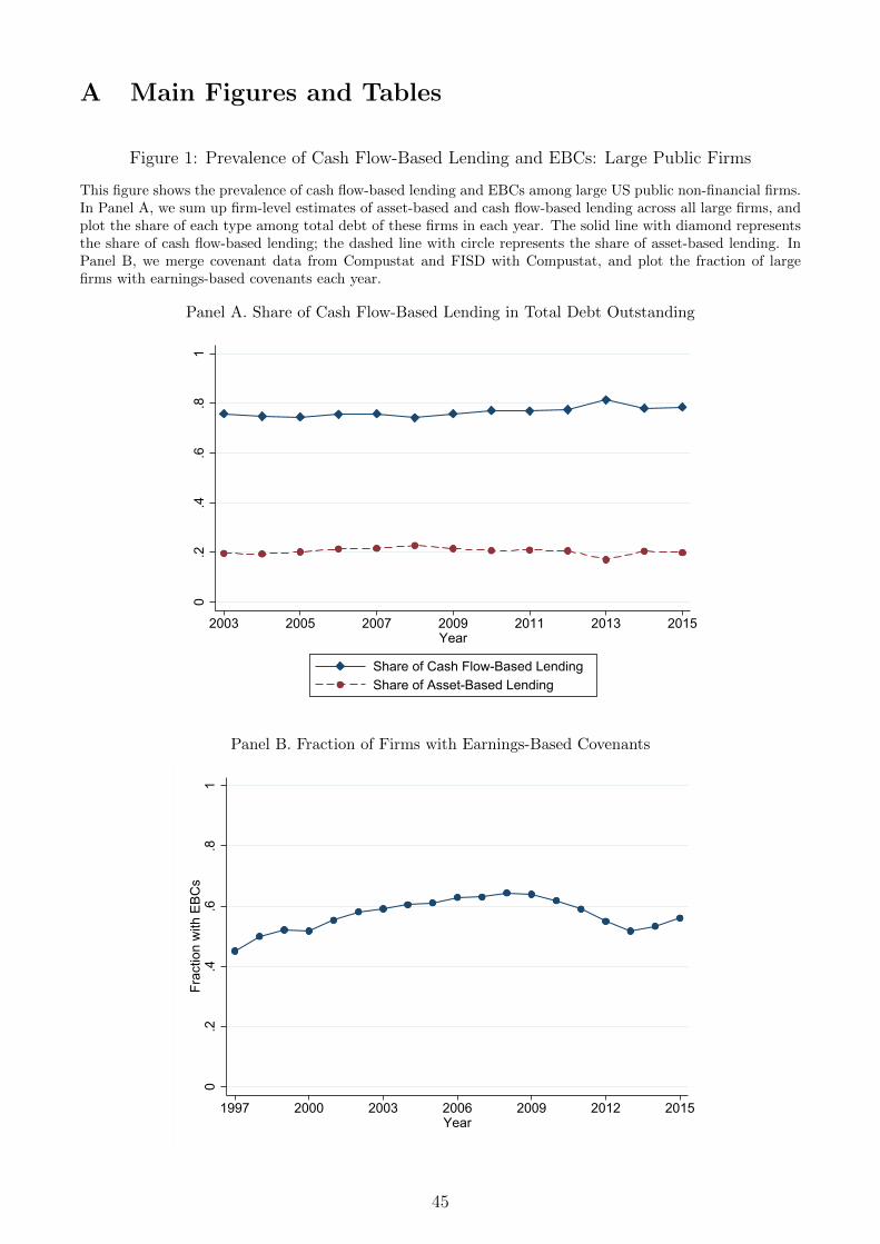
A Main Figures and Tables
Figure 1: Prevalence of Cash Flow-Based Lending and EBCs: Large Public Firms
This figure shows the prevalence of cash flow-based lending and EBCs among large US public non-financial firms.In Panel A, we sum up firm-level estimates of asset-based and cash flow-based lending across all large firms, andplot the share of each type among total debt of these firms in each year. The solid line with diamond representsthe share of cash flow-based lending; the dashed line with circle represents the share of asset-based lending. InPanel B, we merge covenant data from Compustat and FISD with Compustat, and plot the fraction of largefirms with earnings-based covenants each year.
Panel A. Share of Cash Flow-Based Lending in Total Debt Outstanding
0.2
.4.6
.81
2003 2005 2007 2009 2011 2013 2015Year
Share of Cash Flow-Based LendingShare of Asset-Based Lending
Panel B. Fraction of Firms with Earnings-Based Covenants
0.2
.4.6
.81
Frac
tion
with
EBC
s
1997 2000 2003 2006 2009 2012 2015Year
45
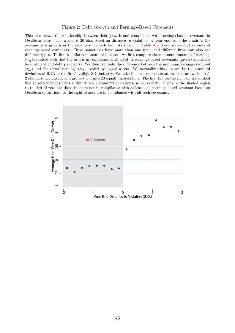
Figure 2: Debt Growth and Earnings-Based Covenants
This plot shows the relationship between debt growth and compliance with earnings-based covenants inDealScan loans. The x-axis is 20 bins based on distance to violation by year end, and the y-axis is theaverage debt growth in the next year in each bin. As shown in Table A5, there are several variants ofearnings-based covenants. Firms sometimes have more than one type, and different firms can also usedifferent types. To find a uniform measure of distance, we first compute the minimum amount of earnings(πit) required such that the firm is in compliance with all of its earnings-based covenants (given the currentlevel of debt and debt payments). We then compute the difference between the minimum earnings required(πit) and the actual earnings (πit), scaled by lagged assets. We normalize this distance by the standarddeviation of ROA in the firm’s 2-digit SIC industry. We take the firm-year observations that are within +/-2 standard deviations, and group them into 20 equally spaced bins. The first bin on the right on the dashedline at zero includes firms within 0 to 0.2 standard deviations, so on so forth. Firms in the shaded regionto the left of zero are those that are not in compliance with at least one earnings-based covenant based onDealScan data; those to the right of zero are in compliance with all such covenants.
In Violation
-.1-.0
50
.05
.1.1
5Av
erag
e N
ext Y
ear D
ebt G
row
th
-2 -1 0 1 2Year End Distance to Violation (S.D.)
46
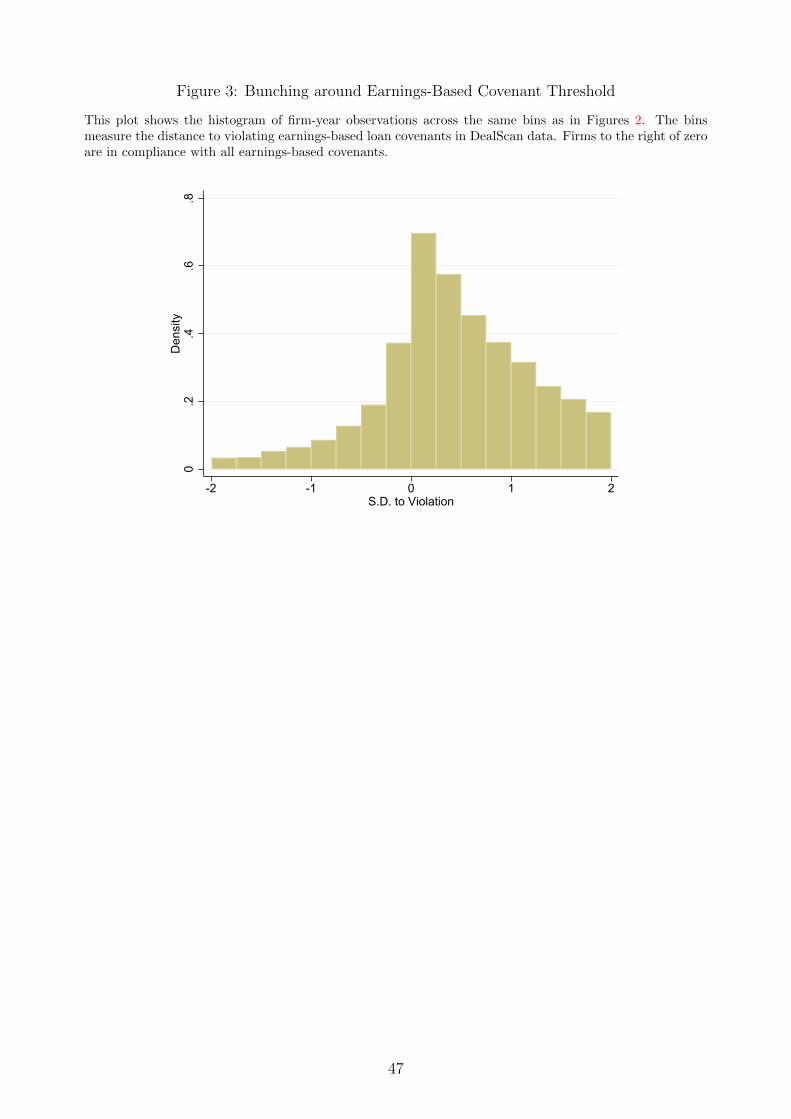
Figure 3: Bunching around Earnings-Based Covenant Threshold
This plot shows the histogram of firm-year observations across the same bins as in Figures 2. The binsmeasure the distance to violating earnings-based loan covenants in DealScan data. Firms to the right of zeroare in compliance with all earnings-based covenants.
0.2
.4.6
.8D
ensi
ty
-2 -1 0 1 2S.D. to Violation
47
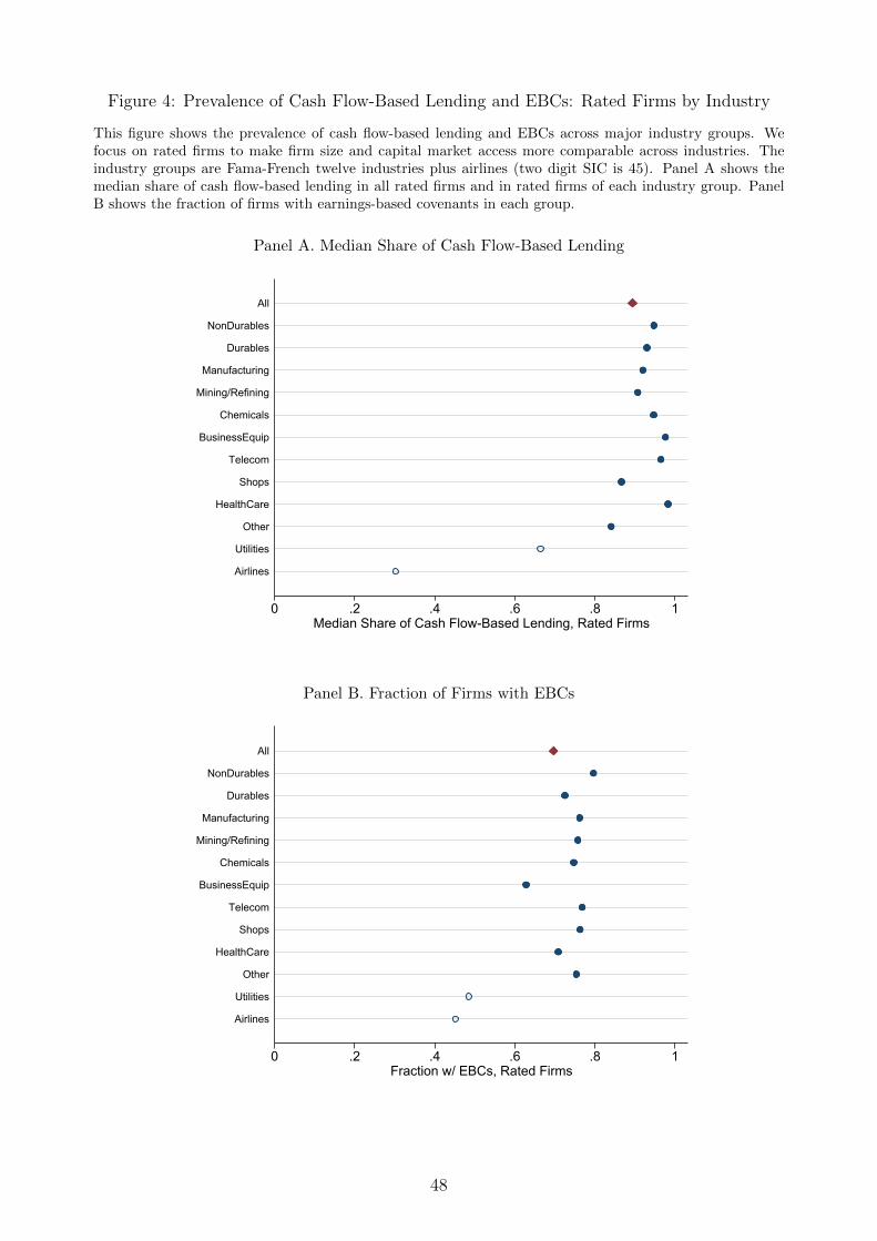
Figure 4: Prevalence of Cash Flow-Based Lending and EBCs: Rated Firms by Industry
This figure shows the prevalence of cash flow-based lending and EBCs across major industry groups. Wefocus on rated firms to make firm size and capital market access more comparable across industries. Theindustry groups are Fama-French twelve industries plus airlines (two digit SIC is 45). Panel A shows themedian share of cash flow-based lending in all rated firms and in rated firms of each industry group. PanelB shows the fraction of firms with earnings-based covenants in each group.
Panel A. Median Share of Cash Flow-Based Lending
0 .2 .4 .6 .8 1Median Share of Cash Flow-Based Lending, Rated Firms
Airlines
Utilities
Other
HealthCare
Shops
Telecom
BusinessEquip
Chemicals
Mining/Refining
Manufacturing
Durables
NonDurables
All
Panel B. Fraction of Firms with EBCs
0 .2 .4 .6 .8 1Fraction w/ EBCs, Rated Firms
Airlines
Utilities
Other
HealthCare
Shops
Telecom
BusinessEquip
Chemicals
Mining/Refining
Manufacturing
Durables
NonDurables
All
48

Figure 5: Property Price Cycle and Corporate Debt Cycle: Japan vs. US
This plot shows the dynamics of non-financial corporate debt and household debt over the property pricecycle in Japan (1975 to 2005) and the US (1990 to 2015). In each plot, the green dashed line is the realestate price index in each country. The blue line with circles is non-financial corporate debt scaled by GDP.The red ling is household debt scaled by GDP. The real estate price index in Japan uses urban land priceindex from the Statistic Bureau in the Ministry of Internal Affairs and Communications. The real estateprice index in the US uses the Case-Shiller price index. The debt data are from the BIS database on creditto the non-financial sector.
Panel A. Japan
4050
6070
Hou
seho
ld D
ebt/G
DP
5070
9011
013
015
0
1975 1980 1985 1990 1995 2000 2005Year
NF Corporate Debt/GDP Household Debt/GDPReal Estate Price Index
Panel B. US
6070
8090
100
Hou
seho
ld D
ebt/G
DP
5070
9011
013
015
0
1990 1995 2000 2005 2010 2015Year
NF Corporate Debt/GDP Household Debt/GDPReal Estate Price Index
49
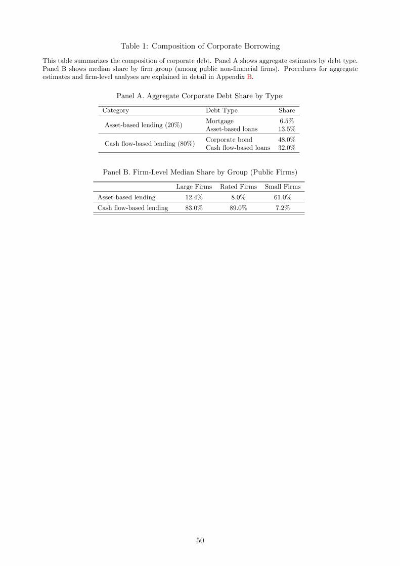
Table 1: Composition of Corporate Borrowing
This table summarizes the composition of corporate debt. Panel A shows aggregate estimates by debt type.Panel B shows median share by firm group (among public non-financial firms). Procedures for aggregateestimates and firm-level analyses are explained in detail in Appendix B.
Panel A. Aggregate Corporate Debt Share by Type:
Category Debt Type Share
Asset-based lending (20%)Mortgage 6.5%Asset-based loans 13.5%
Cash flow-based lending (80%)Corporate bond 48.0%Cash flow-based loans 32.0%
Panel B. Firm-Level Median Share by Group (Public Firms)
Large Firms Rated Firms Small Firms
Asset-based lending 12.4% 8.0% 61.0%
Cash flow-based lending 83.0% 89.0% 7.2%
50

Table 2: Summary Statistics of US Non-Financial Firms
Summary statistics of non-financial firm samples. Panel A shows statistics for large firms with EBCs. Large firms arethose with size (assets) above Compustat median, and EBCs are based on DealScan and FISD data. Mean, median,standard deviation, and selected percentiles are presented. Panel B shows statistics for several firm groups that are notbound by EBCs, including large firms without earnings-based covenants (primarily use cash flow-based lending but arefar from constraints), as well as small firms, low margin firms, and airlines and utilities that rely more on asset-basedlending. Medians are presented for each group. EBITDA is earnings before interest, taxes, and depreciation. OCFis net cash receipts from operations. MTB is market equity to book equity. Q is calculated as the sum of marketvalue of equity and book value of debt, divided by book assets. EDF is expected default frequency. AR stands foraccounts receivable, PPE is the book value of property, plant, and equipment, CAPX is capital expenditures (spendingon property, plant, and equipment). As is customary, flow variables are normalized by lagged assets and stock variablesare normalized by contemporaneous assets throughout the paper. CFL share is median share of cash flow-based lendingin each firm group. The sample period is 1996 to 2015 because comprehensive data on financial covenants from DealScanbegan in 1996.
Panel A. Large Firms w/ EBCs
Variable p25 p50 p75 mean s.d. N
Log assets 6.36 7.16 8.15 7.33 1.33 17,458Log market cap 5.94 6.91 7.95 6.95 1.57 17,458EBITDA 68.39 172.15 464.44 611.98 2110.27 17,458EBITDA/l.assets 0.09 0.13 0.19 0.14 0.09 17,458EBITDA/sales 0.08 0.14 0.21 0.14 0.52 17,458Debt/EBITDA 1.03 2.18 3.80 2.70 3.49 17,458Debt/assets 0.17 0.29 0.43 0.31 0.22 17,458EDF 0.00 0.00 0.07 0.13 0.26 17,458Q 0.79 1.06 1.54 1.30 0.87 17,458MTB 1.13 1.86 3.00 2.44 2.89 17,150OCF/l.assets 0.08 0.12 0.16 0.12 0.08 17,445Cash/assets 0.02 0.05 0.12 0.09 0.10 17,458PPE/assets 0.13 0.26 0.48 0.32 0.24 17,458Inventory/assets 0.01 0.08 0.18 0.12 0.12 17,458AR/assets 0.07 0.12 0.20 0.15 0.11 17,458Intangible/assets 0.05 0.16 0.34 0.22 0.20 17,458Net LT debt issuance/l.assets -0.02 0.00 0.05 0.03 0.15 16,186CAPX/l.assets 0.02 0.04 0.07 0.06 0.07 17,371R&D/l.assets 0.00 0.01 0.04 0.03 0.05 8,826CFL share 0.46 0.88 0.99 0.69 0.36 10,855
Panel B. Other Firm Groups
Large w/o EBCs Small Low Margin Air & UtilitiesVariable p50 N p50 N p50 N p50 N
Log assets 6.85 11,382 4.09 22,336 5.08 25,676 7.98 2,584Log market cap 7.05 11,382 4.08 22,336 4.88 25,676 7.18 2,584EBITDA 119.58 11,382 2.19 22,336 5.37 25,676 282.15 2,584EBITDA/l.assets 0.12 11,382 0.06 22,336 0.06 25,676 0.10 2,584EBITDA/sales 0.14 11,382 0.04 22,336 0.03 25,676 0.21 2,584Debt/EBITDA 0.99 11,382 0.00 22,336 0.48 25,676 3.61 2,584Debt/assets 0.18 11,382 0.07 22,336 0.18 25,676 0.36 2,584EDF 0.00 11,382 0.01 22,336 0.02 25,676 0.00 2,584Q 1.25 11,382 1.23 22,336 0.99 25,676 0.86 2,584MTB 2.07 11,382 1.78 22,336 1.55 25,676 1.63 2,584OCF/l.assets 0.11 11,377 0.05 22,289 0.06 25,631 0.10 2,580Cash/assets 0.13 11,382 0.19 22,336 0.12 25,676 0.02 2,584PPE/assets 0.21 11,382 0.13 22,336 0.17 25,676 0.63 2,584Inventory/assets 0.06 11,382 0.08 22,336 0.07 25,676 0.02 2,584AR/assets 0.11 11,382 0.15 22,336 0.13 25,676 0.06 2,584Intangible/assets 0.08 11,382 0.04 22,336 0.07 25,676 0.02 2,584Net LT debt issuance/l.assets 0.00 10,778 0.00 21,166 0.00 24,151 0.00 2,518CAPX/l.assets 0.04 11,309 0.03 22,150 0.03 25,488 0.07 2,569R&D/l.assets 0.05 7,085 0.08 15,485 0.07 16,474 0.01 89CFL share 0.88 5,277 0.00 8,634 0.47 12,256 0.66 1,531
51

Table 3: Debt Issuance and Investment Activities: Large Firms w/ EBCs
Firm-level annual regressions of debt issuance and investment activities:Yit = αi + ηt + βEBITDAit + κOCFit +X ′itγ + εit
In Panel A the outcome variable Yit is net debt issuance. In Columns (1) and (2) Yit is our main debt issuancemeasure: net debt issuance in year t from the statement of cash flows, calculated as issuance minus reduction oflong-term debt (Compustat item DLTIS - DLTR), normalized by assets at the end of year t−1. In Columns (3) to (4)Yit is changes in total book debt in year t. In Columns (5) to (8), Yit is changes in both secured debt and unsecureddebt, using data from CapitalIQ. In Panel B, the outcome variable Yit is investment activities. In Columns (1) and(2), Yit is capital expenditures (Compustat variable CAPX, which covers purchases of plant, property, and equipment)in year t, normalized by assets at the end of year t− 1. In Columns (3) and (4), Yit is R&D expenditures (Compustatvariable XRD, only non-missing for a subset of firms). EBITDAit is earnings before interest, taxes, depreciation andamortization (Compustat item EBITDA) in year t, normalized by assets at the end of year t− 1. OCFit is net cashreceipts from operating activities (Compustat item OANCF + XINT) in year t. Control variables Xit include Q(market value of equity plus book value of debt normalized by book assets) as of the beginning of year t, stock returnsin year t− 1, as well as cash holdings, book leverage (debt/assets), book PPE (plan, property, equipment), intangibleassets, margin, size (log assets) at the end of t− 1. We also control for net operating assets at the end of year t− 1 asa proxy for accounting quality (Hirshleifer, Hou, Teoh, and Zhang, 2004), and lagged EBITDA to focus on the impactof current EBITDA. Firm fixed effects and year fixed effects are included (R2 does not include fixed effects). Sampleperiod is 1996 to 2015. The sample is restricted to large US non-financial firms that have earnings-based covenantsin year t. Standard errors are clustered by firm and time.
Panel A. Debt Issuance
Net LT Debt Iss. ∆ Book Debt ∆ Unsec. Debt ∆ Secured Debt(1) (2) (3) (4) (5) (6) (7) (8)
EBITDA 0.216*** 0.273*** 0.345*** 0.412*** 0.209*** 0.232*** 0.103*** 0.125***(0.030) (0.034) (0.039) (0.042) (0.037) (0.041) (0.031) (0.033)
OCF -0.111*** -0.135*** -0.048 -0.045*(0.033) (0.045) (0.033) (0.027)
Q 0.010** 0.011** 0.004 0.005 0.010** 0.011** 0.005 0.005(0.005) (0.005) (0.005) (0.005) (0.004) (0.004) (0.005) (0.005)
Past 12m stock ret -0.003 -0.003 0.002 0.001 0.002 0.002 -0.008*** -0.008***(0.003) (0.003) (0.003) (0.003) (0.003) (0.003) (0.003) (0.002)
L.Cash holding -0.033 -0.033 0.039 0.039 -0.117*** -0.117*** 0.052 0.052(0.043) (0.044) (0.051) (0.052) (0.044) (0.043) (0.045) (0.045)
Controls Y Y Y Y Y Y Y YFirm FE Y Y Y Y Y Y Y YYear FE Y Y Y Y Y Y Y YObs 15,642 15,642 15,576 15,576 11,693 11,693 11,678 11,678R2 0.114 0.116 0.152 0.154 0.069 0.069 0.030 0.030
Standard errors in parentheses, clustered by firm and time
Panel B. Investment Activities
CAPX R&D(1) (2) (3) (4)
EBITDA 0.129*** 0.101*** 0.031*** 0.035***(0.017) (0.019) (0.012) (0.013)
OCF 0.053*** -0.007(0.013) (0.011)
Q 0.011*** 0.011*** 0.004*** 0.004***(0.002) (0.002) (0.002) (0.002)
Past 12m stock ret 0.004* 0.004* -0.003*** -0.003***(0.002) (0.002) (0.001) (0.001)
L.Cash holding 0.015 0.015 -0.005 -0.004(0.013) (0.013) (0.012) (0.012)
Controls Y Y Y YFirm FE Y Y Y YYear FE Y Y Y YObs 16,907 16,907 8,588 8,586R2 0.156 0.160 0.108 0.108
Standard errors in parentheses, clustered by firm and time
52

Table 4: Debt Issuance and Investment Activities: Firms w/ Low Prevalence of EBCs
Firm-level annual panel regressions of debt issuance and investment activities on EBITDA:Yit = αi + ηt + βEBITDAit + κOCFit +X ′itγ + εit
The regressions are the same as those in Table 3. In Panel A, the outcome variable is net long-term debt issuance; inPanel B, the outcome variable is capital expenditures. Results are presented for several groups not bound by EBCs:large firms without earnings-based covenants, which use cash flow-based lending but have lower debt and are far fromconstraints; small firms, which have low prevalence of cash flow-based lending and EBCs; low margin firms, whichhave low prevalence of cash flow-based lending and EBCs; airlines and utilities, which have low prevalence of cashflow-based lending and EBCs. Sample period is 1996 to 2015. Standard errors are clustered by firm and time.
Panel A. Net LT Debt Issuance
Large w/o EBCs Small Low Margin Air & Utilities(1) (2) (3) (4) (5) (6) (7) (8)
EBITDA -0.059*** 0.023 -0.019*** 0.001 -0.025*** -0.001 -0.093** -0.059(0.021) (0.027) (0.007) (0.009) (0.008) (0.010) (0.045) (0.061)
OCF -0.127*** -0.033*** -0.039*** -0.050(0.027) (0.011) (0.010) (0.079)
Q 0.007*** 0.007*** 0.004*** 0.004*** 0.007*** 0.007*** 0.042** 0.044**(0.003) (0.002) (0.001) (0.001) (0.002) (0.002) (0.018) (0.019)
Past 12m stock ret 0.001 0.001 0.002 0.002 0.003 0.003 0.003 0.002(0.004) (0.004) (0.002) (0.002) (0.002) (0.002) (0.010) (0.010)
L.Cash holding -0.048** -0.042* -0.055*** -0.059*** -0.071*** -0.076*** -0.109** -0.130**(0.024) (0.024) (0.016) (0.017) (0.019) (0.020) (0.055) (0.063)
Controls Y Y Y Y Y Y Y YFirm FE Y Y Y Y Y Y Y YYear FE Y Y Y Y Y Y Y YObs 10,137 10,136 20,153 20,129 22,557 22,534 2,475 2,474R2 0.073 0.078 0.029 0.030 0.036 0.038 0.087 0.088
Standard errors in parentheses, clustered by firm and time
Panel B. CAPX Investment
Large w/o EBCs Small Low Margin Air & Utilities(1) (2) (3) (4) (5) (6) (7) (8)
EBITDA 0.053*** 0.033* 0.001 -0.002 0.002 -0.004 0.079 0.025(0.012) (0.019) (0.004) (0.004) (0.005) (0.004) (0.049) (0.046)
OCF 0.024** 0.005 0.011** 0.158***(0.011) (0.004) (0.005) (0.038)
Q 0.004*** 0.004*** 0.006*** 0.006*** 0.006*** 0.006*** 0.029*** 0.026***(0.001) (0.001) (0.001) (0.001) (0.001) (0.001) (0.010) (0.010)
Past 12m stock ret 0.006*** 0.006*** 0.004*** 0.004*** 0.004*** 0.004*** 0.007 0.006(0.002) (0.002) (0.001) (0.001) (0.001) (0.001) (0.006) (0.006)
L.Cash holding -0.019* -0.019* 0.005 0.006 0.002 0.003 -0.018 -0.004(0.011) (0.011) (0.006) (0.006) (0.005) (0.005) (0.056) (0.056)
Controls Y Y Y Y Y Y Y YFirm FE Y Y Y Y Y Y Y YYear FE Y Y Y Y Y Y Y YObs 10,683 10,681 21,249 21,222 24,045 24,020 2,535 2,534R2 0.107 0.108 0.043 0.043 0.046 0.047 0.122 0.144
Standard errors in parentheses, clustered by firm and time
53
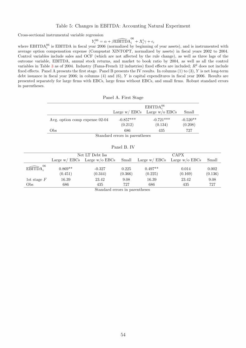
Table 5: Changes in EBITDA: Accounting Natural Experiment
Cross-sectional instrumental variable regression
Y 06i = α+ β EBITDA
06
i +X ′iγ + εiwhere EBITDA06
i is EBITDA in fiscal year 2006 (normalized by beginning of year assets), and is instrumented withaverage option compensation expense (Compustat XINTOPT, normalized by assets) in fiscal years 2002 to 2004.Control variables include sales and OCF (which are not affected by the rule change), as well as three lags of theoutcome variable, EBITDA, annual stock returns, and market to book ratio by 2004, as well as all the controlvariables in Table 3 as of 2004. Industry (Fama-French 12 industries) fixed effects are included; R2 does not includefixed effects. Panel A presents the first stage. Panel B presents the IV results. In columns (1) to (3), Y is net long-termdebt issuance in fiscal year 2006; in columns (4) and (6), Y is capital expenditures in fiscal year 2006. Results arepresented separately for large firms with EBCs, large firms without EBCs, and small firms. Robust standard errorsin parentheses.
Panel A. First Stage
EBITDA06i
Large w/ EBCs Large w/o EBCs Small
Avg. option comp expense 02-04 -0.857*** -0.721*** -0.520**(0.212) (0.134) (0.208)
Obs 686 435 727Standard errors in parentheses
Panel B. IV
Net LT Debt Iss CAPXLarge w/ EBCs Large w/o EBCs Small Large w/ EBCs Large w/o EBCs Small
EBITDA06
i 0.869** -0.327 0.225 0.497** 0.014 0.002(0.451) (0.344) (0.366) (0.225) (0.169) (0.136)
1st stage F 16.39 23.42 9.08 16.39 23.42 9.08Obs 686 435 727 686 435 727
Standard errors in parentheses
54
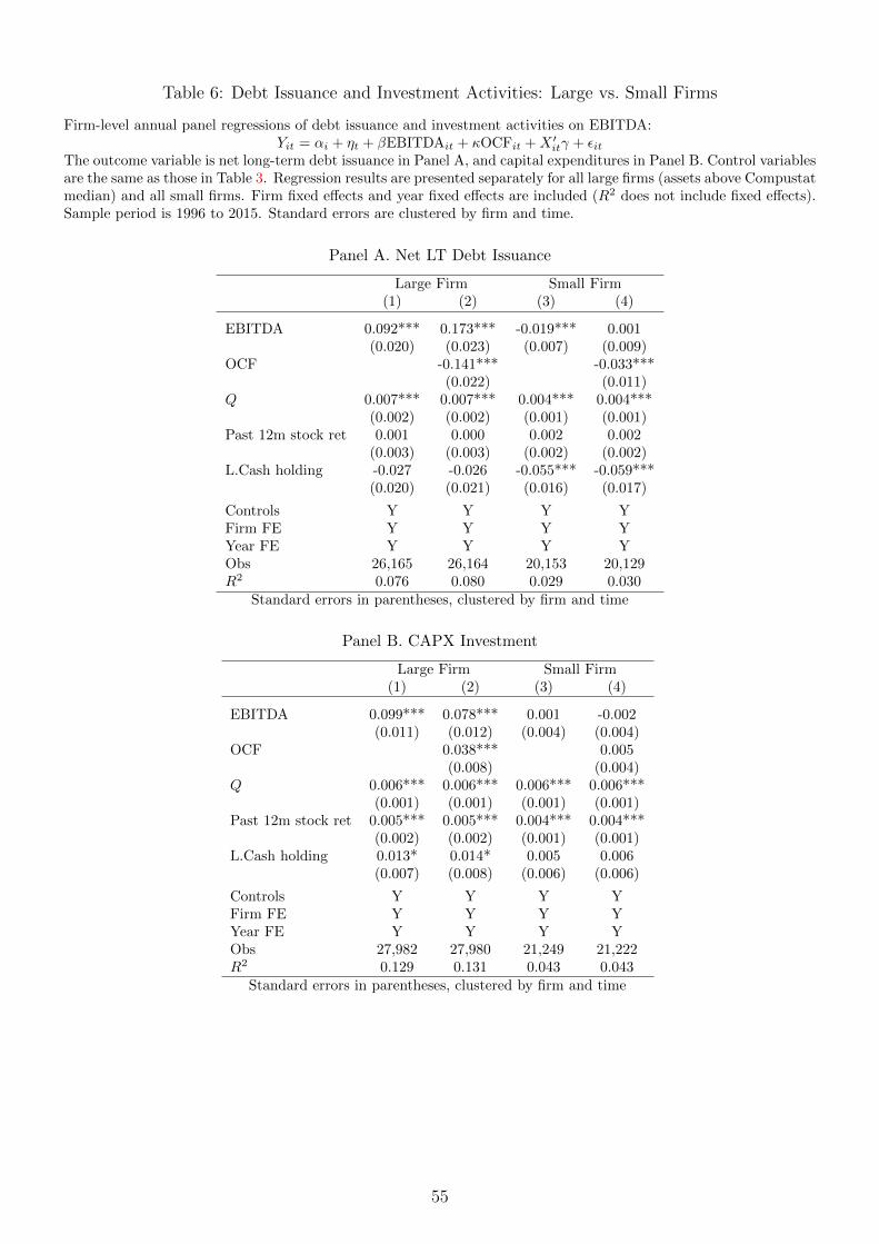
Table 6: Debt Issuance and Investment Activities: Large vs. Small Firms
Firm-level annual panel regressions of debt issuance and investment activities on EBITDA:Yit = αi + ηt + βEBITDAit + κOCFit +X ′itγ + εit
The outcome variable is net long-term debt issuance in Panel A, and capital expenditures in Panel B. Control variablesare the same as those in Table 3. Regression results are presented separately for all large firms (assets above Compustatmedian) and all small firms. Firm fixed effects and year fixed effects are included (R2 does not include fixed effects).Sample period is 1996 to 2015. Standard errors are clustered by firm and time.
Panel A. Net LT Debt Issuance
Large Firm Small Firm(1) (2) (3) (4)
EBITDA 0.092*** 0.173*** -0.019*** 0.001(0.020) (0.023) (0.007) (0.009)
OCF -0.141*** -0.033***(0.022) (0.011)
Q 0.007*** 0.007*** 0.004*** 0.004***(0.002) (0.002) (0.001) (0.001)
Past 12m stock ret 0.001 0.000 0.002 0.002(0.003) (0.003) (0.002) (0.002)
L.Cash holding -0.027 -0.026 -0.055*** -0.059***(0.020) (0.021) (0.016) (0.017)
Controls Y Y Y YFirm FE Y Y Y YYear FE Y Y Y YObs 26,165 26,164 20,153 20,129R2 0.076 0.080 0.029 0.030
Standard errors in parentheses, clustered by firm and time
Panel B. CAPX Investment
Large Firm Small Firm(1) (2) (3) (4)
EBITDA 0.099*** 0.078*** 0.001 -0.002(0.011) (0.012) (0.004) (0.004)
OCF 0.038*** 0.005(0.008) (0.004)
Q 0.006*** 0.006*** 0.006*** 0.006***(0.001) (0.001) (0.001) (0.001)
Past 12m stock ret 0.005*** 0.005*** 0.004*** 0.004***(0.002) (0.002) (0.001) (0.001)
L.Cash holding 0.013* 0.014* 0.005 0.006(0.007) (0.008) (0.006) (0.006)
Controls Y Y Y YFirm FE Y Y Y YYear FE Y Y Y YObs 27,982 27,980 21,249 21,222R2 0.129 0.131 0.043 0.043
Standard errors in parentheses, clustered by firm and time
55
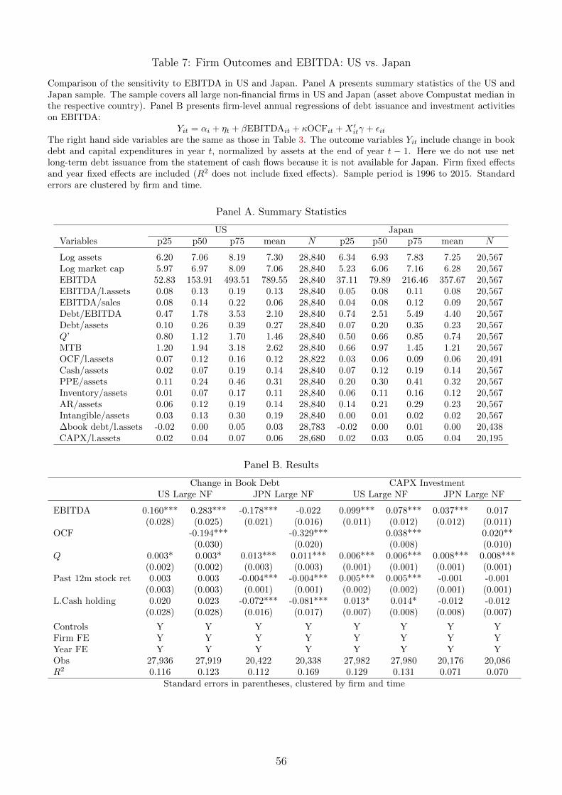
Table 7: Firm Outcomes and EBITDA: US vs. Japan
Comparison of the sensitivity to EBITDA in US and Japan. Panel A presents summary statistics of the US andJapan sample. The sample covers all large non-financial firms in US and Japan (asset above Compustat median inthe respective country). Panel B presents firm-level annual regressions of debt issuance and investment activitieson EBITDA:
Yit = αi + ηt + βEBITDAit + κOCFit +X ′itγ + εitThe right hand side variables are the same as those in Table 3. The outcome variables Yit include change in bookdebt and capital expenditures in year t, normalized by assets at the end of year t − 1. Here we do not use netlong-term debt issuance from the statement of cash flows because it is not available for Japan. Firm fixed effectsand year fixed effects are included (R2 does not include fixed effects). Sample period is 1996 to 2015. Standarderrors are clustered by firm and time.
Panel A. Summary Statistics
VariablesUS Japan
p25 p50 p75 mean N p25 p50 p75 mean N
Log assets 6.20 7.06 8.19 7.30 28,840 6.34 6.93 7.83 7.25 20,567Log market cap 5.97 6.97 8.09 7.06 28,840 5.23 6.06 7.16 6.28 20,567EBITDA 52.83 153.91 493.51 789.55 28,840 37.11 79.89 216.46 357.67 20,567EBITDA/l.assets 0.08 0.13 0.19 0.13 28,840 0.05 0.08 0.11 0.08 20,567EBITDA/sales 0.08 0.14 0.22 0.06 28,840 0.04 0.08 0.12 0.09 20,567Debt/EBITDA 0.47 1.78 3.53 2.10 28,840 0.74 2.51 5.49 4.40 20,567Debt/assets 0.10 0.26 0.39 0.27 28,840 0.07 0.20 0.35 0.23 20,567Q’ 0.80 1.12 1.70 1.46 28,840 0.50 0.66 0.85 0.74 20,567MTB 1.20 1.94 3.18 2.62 28,840 0.66 0.97 1.45 1.21 20,567OCF/l.assets 0.07 0.12 0.16 0.12 28,822 0.03 0.06 0.09 0.06 20,491Cash/assets 0.02 0.07 0.19 0.14 28,840 0.07 0.12 0.19 0.14 20,567PPE/assets 0.11 0.24 0.46 0.31 28,840 0.20 0.30 0.41 0.32 20,567Inventory/assets 0.01 0.07 0.17 0.11 28,840 0.06 0.11 0.16 0.12 20,567AR/assets 0.06 0.12 0.19 0.14 28,840 0.14 0.21 0.29 0.23 20,567Intangible/assets 0.03 0.13 0.30 0.19 28,840 0.00 0.01 0.02 0.02 20,567∆book debt/l.assets -0.02 0.00 0.05 0.03 28,783 -0.02 0.00 0.01 0.00 20,438CAPX/l.assets 0.02 0.04 0.07 0.06 28,680 0.02 0.03 0.05 0.04 20,195
Panel B. Results
Change in Book Debt CAPX InvestmentUS Large NF JPN Large NF US Large NF JPN Large NF
EBITDA 0.160*** 0.283*** -0.178*** -0.022 0.099*** 0.078*** 0.037*** 0.017(0.028) (0.025) (0.021) (0.016) (0.011) (0.012) (0.012) (0.011)
OCF -0.194*** -0.329*** 0.038*** 0.020**(0.030) (0.020) (0.008) (0.010)
Q 0.003* 0.003* 0.013*** 0.011*** 0.006*** 0.006*** 0.008*** 0.008***(0.002) (0.002) (0.003) (0.003) (0.001) (0.001) (0.001) (0.001)
Past 12m stock ret 0.003 0.003 -0.004*** -0.004*** 0.005*** 0.005*** -0.001 -0.001(0.003) (0.003) (0.001) (0.001) (0.002) (0.002) (0.001) (0.001)
L.Cash holding 0.020 0.023 -0.072*** -0.081*** 0.013* 0.014* -0.012 -0.012(0.028) (0.028) (0.016) (0.017) (0.007) (0.008) (0.008) (0.007)
Controls Y Y Y Y Y Y Y YFirm FE Y Y Y Y Y Y Y YYear FE Y Y Y Y Y Y Y YObs 27,936 27,919 20,422 20,338 27,982 27,980 20,176 20,086R2 0.116 0.123 0.112 0.169 0.129 0.131 0.071 0.070
Standard errors in parentheses, clustered by firm and time
56

Table 8: Summary Statistics: Firm Property Value
Summary statistics of firms in the samples with market value of real estate measures. The column labeled“Method 1” refers to the sample where market value of real estate estimates are available using Method 1described in Section 4.1 and Appendix G, which follows the traditional procedure (Chaney et al., 2012). Thecolumn labeled “Method 2” refers to the sample where market value of real estate estimates are availableusing Method 2 described in Section 4.1 and Appendix G, which uses hand collected information from 10-Kfilings. The column labeled “All w/ RE” includes all non-financial firms with non-zero real estate holdings.Panel A displays statistics for the period 2002 to 2015 (sample period in Table 9), for which we have firm-level measures of asset-based and cash flow-based lending. Panel B displays additional statistics for theperiod 2007 to 2019 (sample period in Table 10). ∆RE07−09
06 /sssets06 is the gain/loss on 2006 real estateholdings during the crisis, normalized by assets in 2006. ∆P 07−09(HQ) is the percentage change in propertyprice index in headquarters CBSA from 2007 to 2009. The remaining statistics are changes in EBITDA, netlong-term debt issuance, and capital expenditures between 2007 and 2009, normalized by assets in 2006.
SampleMethod 1 Method 2 All w/ RE
Panel A. 2002—2015
Market Value RE/assets 0.21 0.13 -Market Value RE/market cap 0.21 0.12 -Book PPE/assets 0.25 0.21 0.25EBITDA/l.assets 0.14 0.13 0.12Q 1.15 1.14 1.10Debt/assets 0.22 0.19 0.24Log assets 7.08 6.30 6.84Asset-based lending/debt 0.12 0.25 0.22Cash flow-based lending/debt 0.85 0.66 0.74Asset-based lending/assets 0.02 0.02 0.03Cash flow-based lending/assets 0.16 0.09 0.14Net LT Debt issuance/assets 0.00 0.00 0.00CAPX/l.assets 0.04 0.04 0.04Fraction of large firms 0.76 0.63 0.71Fraction w/ EBCs 0.60 0.55 0.56
Panel B. 2007—2009
∆RE07−0906 /assets06 -0.01 -0.01 -
∆P 07−09(HQ) -0.07 -0.08 -0.07∆EBITDA07−09
06 /assets06 -0.02 -0.01 -0.01
∆Net LT Debt Iss07−0906 /assets06 0.00 0.00 0.00∆CAPX07−09
06 /assets06 -0.01 -0.01 -0.01
57
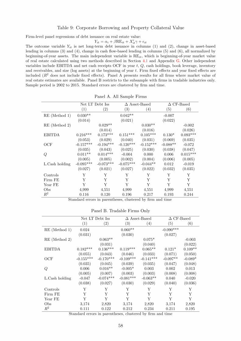
Table 9: Corporate Borrowing and Property Collateral Value
Firm-level panel regressions of debt issuance on real estate value:Yit = αi + βREit +X ′itγ + εit
The outcome variable Yit is net long-term debt issuance in columns (1) and (2), change in asset-basedlending in columns (3) and (4), change in cash flow-based lending in columns (5) and (6), all normalized bybeginning-of-year assets. The main independent variable is REit, which is beginning-of-year market valueof real estate calculated using two methods described in Section 4.1 and Appendix G. Other independentvariables include EBITDA and net cash receipts OCF in year t, Q, cash holdings, book leverage, inventoryand receivables, and size (log assets) at the beginning of year t. Firm fixed effects and year fixed effects areincluded (R2 does not include fixed effects). Panel A presents results for all firms where market value ofreal estate estimates are available. Panel B restricts to the subsample with firms in tradable industries only.Sample period is 2002 to 2015. Standard errors are clustered by firm and time.
Panel A. All Sample Firms
Net LT Debt Iss ∆ Asset-Based ∆ CF-Based(1) (2) (3) (4) (5) (6)
RE (Method 1) 0.030** 0.042** -0.007(0.014) (0.021) (0.022)
RE (Method 2) 0.029** 0.030** -0.002(0.014) (0.016) (0.026)
EBITDA 0.216*** 0.173*** 0.151*** 0.105*** 0.130* 0.093***(0.053) (0.029) (0.040) (0.031) (0.069) (0.035)
OCF -0.157*** -0.194*** -0.120*** -0.152*** -0.088** -0.072(0.035) (0.043) (0.025) (0.030) (0.038) (0.047)
Q 0.011** 0.014*** -0.004 0.000 0.006 0.015***(0.005) (0.005) (0.002) (0.004) (0.006) (0.005)
L.Cash holding -0.095*** -0.073*** -0.075*** -0.044** 0.012 -0.019(0.027) (0.021) (0.027) (0.022) (0.032) (0.035)
Controls Y Y Y Y Y YFirm FE Y Y Y Y Y YYear FE Y Y Y Y Y YObs 4,999 4,551 4,999 4,551 4,999 4,551R2 0.116 0.120 0.196 0.217 0.193 0.244
Standard errors in parentheses, clustered by firm and time
Panel B. Tradable Firms Only
Net LT Debt Iss ∆ Asset-Based ∆ CF-Based(1) (2) (3) (4) (5) (6)
RE (Method 1) 0.024 0.060** -0.090***(0.031) (0.030) (0.027)
RE (Method 2) 0.063** 0.075* -0.003(0.031) (0.040) (0.022)
EBITDA 0.182*** 0.136*** 0.119*** 0.065** 0.121* 0.109**(0.055) (0.043) (0.046) (0.033) (0.071) (0.050)
OCF -0.155*** -0.170*** -0.109*** -0.141*** -0.097** -0.089*(0.035) (0.045) (0.039) (0.035) (0.047) (0.048)
Q 0.006 0.016** -0.005* 0.003 0.002 0.013(0.005) (0.007) (0.003) (0.003) (0.008) (0.008)
L.Cash holding -0.047 -0.074*** -0.081*** -0.063** 0.040 -0.020(0.038) (0.027) (0.030) (0.029) (0.040) (0.036)
Controls Y Y Y Y Y YFirm FE Y Y Y Y Y YYear FE Y Y Y Y Y YObs 3,174 2,820 3,174 2,820 3,174 2,820R2 0.111 0.122 0.212 0.234 0.211 0.195
Standard errors in parentheses, clustered by firm and time
58
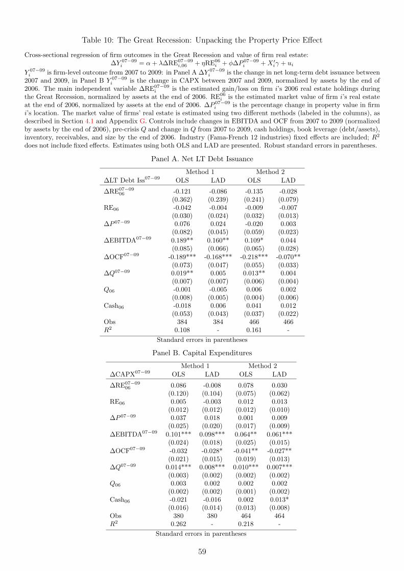
Table 10: The Great Recession: Unpacking the Property Price Effect
Cross-sectional regression of firm outcomes in the Great Recession and value of firm real estate:∆Y 07−09
i = α+ λ∆RE07−09i,06 + ηRE06
i + φ∆P 07−09i +X ′iγ + ui
Y 07−09i is firm-level outcome from 2007 to 2009: in Panel A ∆Y 07−09
i is the change in net long-term debt issuance between2007 and 2009, in Panel B Y 07−09
i is the change in CAPX between 2007 and 2009, normalized by assets by the end of2006. The main independent variable ∆RE07−09
i is the estimated gain/loss on firm i’s 2006 real estate holdings duringthe Great Recession, normalized by assets at the end of 2006. RE06
i is the estimated market value of firm i’s real estateat the end of 2006, normalized by assets at the end of 2006. ∆P 07−09
i is the percentage change in property value in firmi’s location. The market value of firms’ real estate is estimated using two different methods (labeled in the columns), asdescribed in Section 4.1 and Appendix G. Controls include changes in EBITDA and OCF from 2007 to 2009 (normalizedby assets by the end of 2006), pre-crisis Q and change in Q from 2007 to 2009, cash holdings, book leverage (debt/assets),inventory, receivables, and size by the end of 2006. Industry (Fama-French 12 industries) fixed effects are included; R2
does not include fixed effects. Estimates using both OLS and LAD are presented. Robust standard errors in parentheses.
Panel A. Net LT Debt Issuance
Method 1 Method 2
∆LT Debt Iss07−09 OLS LAD OLS LAD
∆RE07−0906 -0.121 -0.086 -0.135 -0.028
(0.362) (0.239) (0.241) (0.079)RE06 -0.042 -0.004 -0.009 -0.007
(0.030) (0.024) (0.032) (0.013)∆P 07−09 0.076 0.024 -0.020 0.003
(0.082) (0.045) (0.059) (0.023)∆EBITDA07−09 0.189** 0.160** 0.109* 0.044
(0.085) (0.066) (0.065) (0.028)∆OCF07−09 -0.189*** -0.168*** -0.218*** -0.070**
(0.073) (0.047) (0.055) (0.033)∆Q07−09 0.019** 0.005 0.013** 0.004
(0.007) (0.007) (0.006) (0.004)Q06 -0.001 -0.005 0.006 0.002
(0.008) (0.005) (0.004) (0.006)Cash06 -0.018 0.006 0.041 0.012
(0.053) (0.043) (0.037) (0.022)Obs 384 384 466 466R2 0.108 - 0.161 -
Standard errors in parentheses
Panel B. Capital Expenditures
Method 1 Method 2∆CAPX07−09 OLS LAD OLS LAD
∆RE07−0906 0.086 -0.008 0.078 0.030
(0.120) (0.104) (0.075) (0.062)RE06 0.005 -0.003 0.012 0.013
(0.012) (0.012) (0.012) (0.010)∆P 07−09 0.037 0.018 0.001 0.009
(0.025) (0.020) (0.017) (0.009)∆EBITDA07−09 0.101*** 0.098*** 0.064** 0.061***
(0.024) (0.018) (0.025) (0.015)∆OCF07−09 -0.032 -0.028* -0.041** -0.027**
(0.021) (0.015) (0.019) (0.013)∆Q07−09 0.014*** 0.008*** 0.010*** 0.007***
(0.003) (0.002) (0.002) (0.002)Q06 0.003 0.002 0.002 0.002
(0.002) (0.002) (0.001) (0.002)Cash06 -0.021 -0.016 0.002 0.013*
(0.016) (0.014) (0.013) (0.008)Obs 380 380 464 464R2 0.262 - 0.218 -
Standard errors in parentheses
59

Table 11: Property Price Collapse and Firm Investment: US vs. Japan
This table compares results in Gan (2007)’s analysis of Japanese firms during Japan’s property price collapseand similar specifications using US firms during the Great Recession. The specification follows Table 2column (2) of Gan (2007):
CAPXposti = α+ βREpre
i +X ′iγ + viCAPXpost
i is firm i’s average annual investment rate (CAPX normalized by assets) over a period of time duringthe property price collapse, and the period is labeled in row “Outcome Period.” REpre
i is firm i’s real estateholdings prior to the collapse (normalized by pre-collapse assets). Gan (2007) uses the estimated marketvalue of land holdings in 1989. In the US sample, we use the market value of real estate in 2006 measuredusing methods described in Section 4.1 and Appendix G. Controls Xi include cash flows (contemporaneouswith investment), as well as Q, cash holdings and book leverage (measured prior to the outcome variable).The regression also follows Gan (2007) to include a dummy variable that is equal to one if the firm’s pre-collapse real estate holdings fall into the top industry quartile, and interactions of this dummy with cashflows and cash holdings. Gan (2007) uses least absolute deviation (LAD) estimate, and we report both OLSand LAD estimates.
CAPX InvestmentJapan (Gan 07) US
Outcome Period 1994—1998 2007-2009 2007-2011 2009-2013Specification LAD OLS LAD OLS LAD OLS LAD
RE 1989 -0.165(0.016)
RE 2006 - 0.007 0.014 -0.001 0.007 -0.01 0.004Method 1 - (0.009) (0.008) (0.008) (0.005) (0.009) (0.004)
RE 2006 - 0.007 0.002 0.008 0.005 -0.005 -0.004Method 2 - (0.007) (0.004) (0.007) (0.005) (0.005) (0.005)
Standard errors in parentheses
60

B Cash Flow-Based Lending and Asset-Based Lending
In this section, we explain in detail the categorization of cash flow-based lending and
asset-based lending. We first lay out the main types of debt in each category. We then
describe our categorization procedure in the aggregate and at the firm level.39
Cash Flow-Based Lending
Cash flow-based lending consists of debt where creditors’ payoffs primarily come from
the value of cash flows from firms’ operations, rather than the liquidation value of physical
collateral (both in ordinary course and in bankruptcy). The debt has several features: 1)
it is unsecured, or secured by a lien on the entire corporate entity (substantially all assets,
excluding those pledged for asset-based loans) or by equity, rather than by specific physical
assets; 2) they closely monitor borrower’s cash flows (e.g. through financial covenants), rather
than the liquidation value of physical assets.
In US bankruptcy procedures, claims are grouped into secured claims and unsecured
claims, with secured claims ranking before unsecured claims in priority. The portion of
a secured debt up to the value of its collateral is treated as a secured claim; the rest is
treated as an unsecured claim. For unsecured claims, in both Chapter 11 reorganization and
Chapter 7 liquidation, the payoffs are not closely related to the liquidation value of physical
assets (payoffs depend on the cash flow value from continuing operations in Chapter 11,
and are generally minimal in Chapter 7). For debt secured by the entire corporate entity
or by equity, creditors’ collateral value and payoffs are based on the cash flow value from
continuing operations in Chapter 11. Payoffs in Chapter 7 may be affected by the liquidation
value of physical assets, but they are generally small and Chapter 7 cases are rare for large
firms that extensively use cash-flow based lending (according to CapitalIQ data, more than
90% of large firms’ bankruptcies are resolved through Chapter 11).
There are two main components of cash flow-based lending: corporate bonds and cash
flow-based loans.
1. Corporate bonds
Corporate bonds are generally backed by borrowers’ future cash flows and are com-
monly unsecured. FISD data shows that less than 1% of corporate debt issuance by
US non-financial firms is asset backed. About 10% is secured; a very small portion
(e.g. industrial revenue bonds) is backed by physical assets, while most secured bonds
are still cash flow-based.
2. Cash flow-based loans
Cash flow-based loans comprise of commercial loans that are primarily backed by bor-
rowers’ cash flows. The prototypical cash flow-based loans do not use specific physical
assets as collateral. Rather, the collateral is a lien on the entire corporate entity, and
39In the categorization, we do not include commercial papers, which are short-term unsecured debt forliquidity purposes.
61

the collateral value is calculated based on the cash flows of the borrower. Creditors
perform detailed cash flow analyses, and closely monitor borrowers’ cash flows. These
loans use earnings-based covenants extensively (e.g. debt to EBITDA ratio, interest
coverage ratio). They typically take the form of a term loan and are widely used
among large firms.
Among large firms, revolving lines of credit (“revolver”), is a class of debt that can be
in between cash flow-based lending and asset-based lending. For large firms with high
credit quality, the revolvers are generally unsecured. For those with higher risks, the
revolvers are typically secured by inventory and accounts receivable (and some other
eligible assets). In these cases, the revolvers do rely on physical assets as collateral,
and specify borrowing limits of the revolvers that depend on the liquidation value
of the physical collateral (“borrowing base,” discussed more below). However, due
to institutional reasons the revolvers are typically bundled together with prototypical
cash flow loans (e.g. term loans) in a single loan package, and share the earnings-based
covenants. For small firms, many revolvers are instead stand-alone asset-based loans.
Asset-Based Lending
Asset-based lending consists of debt where creditors’ payoffs in default tie to the liqui-
dation value of physical assets that serve as collateral. The debt has the following features:
1) it is secured by specific physical assets as collateral; 2) it restricts the size of the debt
based on the value of the given collateral, and creditors focus on the liquidation value of the
specific assets that serve as collateral; 3) the debt may also have some liquidity tests, but
place less emphasis on the borrower’s cash flow performance and related financial covenants.
In US bankruptcy procedures, the portion of the debt up to the liquidation value of the
given collateral is considered a secured claim, which is the primary source of recovery for
asset-based lenders; the rest (“under-collateralized” portion) is treated as an unsecured claim.
In Chapter 7, creditors’ payoffs almost entirely come from the liquidation value of the assets;
unsecured claims get no or minimal payments. In Chapter 11, creditors’ secured claims (up
to the collateral value of the assets) can be paid in full;40 they may get some additional
recovery if they are “under-collateralized” and unsecured claims get some payments, but
this portion is typically small in comparison.
The most important components of asset-based lending are commercial mortgages and
business loans secured by specific assets such as inventory, accounts receivable, and certain
types of equipment (often referred to as asset-based loans). We also include capital leases,
but the total amount is small.41
1. Commercial mortgages
40Section 1129(a)(7)(A) of the Bankruptcy Code requires that for a Chapter 11 reorganization to beapproved, it must be established that each secured claim holder would receive at least the amount he/shewould get if the borrower were liquidated under Chapter 7.
41The term “asset-based lending” is sometimes used narrowly to refer to asset-based loans with inventoryand receivables as collateral. Here we use the term more broadly.
62

Commercial mortgages are corporate debt backed by real estate. For larger firms, the
collateral is typically commercial real estate, mostly office buildings/corporate head-
quarters and sometimes retail properties like shopping malls and hotels. Very small
firms may also use residential mortgages.
2. Asset-based loans
Asset-based loans are business (non-mortgage) loans backed by physical assets as col-
lateral, such as inventory, receivable, some machinery and equipment, and some spe-
cialized assets such as oil and gas reserves. Asset-based loans specify a “borrowing
base,” calculated based on the liquidation value of eligible collateral. Creditors regu-
larly monitor the borrowing base and require that the loan size cannot exceed a fraction
of the borrowing base. Asset-based loans can be originated by banks, as well as finance
companies that specialize in lending against specific types of collateral.
3. Capitalized leases
In a capital lease, the leased asset shows up on the asset side of the lessee’s balance
sheet, and the lease shows up on the liability side. Capital leases are often treated
as debt (Compustat includes capitalized lease as part of the debt variable). This
contrasts with operating leases (e.g. rent), in which case the lease and the lease asset
do not appear on the lessee’s balance sheet. A lease is recognized as a capital lease
when the lessee has exposures to the ownership of the asset, e.g. the lease specifies a
transfer of ownership from the lessor to the lessee at the end of the lease period, or that
the lease period covers a substantial amount of the life of the asset. US GAAP specifies
rules about recognizing capital leases. A well known example of capital lease is used in
aircraft financing and studied in Benmelech and Bergman (2011). In this case, a trust
purchases the aircraft, leases it to the airline, and finances the purchase by issuing
secured notes backed by the aircraft. The trust is sometimes set up by the airline, but
is bankruptcy remote. Because the financing of assets in capital leases is often tied
to the assets’ liquidation value, we categorize capital leases as asset-based lending. As
the size of this portion is relatively small (about $70 billion among Compustat public
firms), in the following calculations we merge capital leases with asset-based loans.
B.1 Aggregate Composition
In the following, we estimate the share of cash flow-based and asset-based lending among
aggregate US non-financial corporate debt outstanding. Here we primarily rely on aggregate
sources, so the estimates are not confined to public firms.
Cash Flow-Based Lending: around 80% of debt outstanding
1. Corporate bonds
• Share in total non-financial corporate debt outstanding: 49%
63

• Data source: Flow of Funds, FISD, CapitalIQ
• Calculation: According to Flow of Funds data, corporate bond outstanding by
US non-financial firms is about $4.5 trillion. Based on FISD and CapitalIQ data,
which provide more information on the structure of individual corporate bonds,
only a small portion of corporate bonds are backed by specific physical assets
(<2%). Thus in the aggregate, we categorize all corporate bonds into cash flow-
based lending.
2. Cash flow-based loans
• Share in total non-financial corporate debt outstanding: 32%
• Data sources: DealScan, ABL Advisor, Shared National Credits Program (SNC)
• Calculation: We approximate the volume of cash flow loans using the cash flow-
based portion of syndicated loans, which cover the vast majority of cash flow
loans by dollar volume. We proceed in two steps. We first estimate the share
of cash flow loans versus asset-based loans in syndicated loans, using data from
the DealScan and ABL Advisor. In particular, ABL Advisor reports the volume
of issuance in DealScan that can be classified as asset-base loans, and we can
compare this to the volume of all DealScan issuance to get the asset-based share,
and the remainder is the cash flow-based share. We can alternatively calculate
(directly using DealScan data) the share of DealScan loans that do not have
borrowing base requirements, and the results are very similar. The estimated
share of cash flow loans is roughly 95% (annual syndicated loan issuance is about
$1,500B to $2,000B, of which $60B to $100B is asset-based). We then turn to the
volume of syndicated loans outstanding. Volume outstanding in not included in
DealScan. Thus we instead use data on syndicated loans outstanding from SNC,
and estimate the amount to be about $3 trillion.
Asset-Based Lending: around 20% of debt outstanding
1. Commercial mortgages
• Share in total non-financial debt outstanding: 7%
• Data sources: Flow of Funds
• Calculation: We use commercial mortgage outstanding from the Flow of Funds,
which is around $0.6 trillion.
2. Asset-based loans:
• Share in total non-financial debt outstanding: 12%
• Data sources: DealScan, ABL Advisor, SNC, SBA/Call Report
64

• Calculation: We first estimate asset-based loans to large firms. For this part,
we start with data from DealScan, ABL advisor, and SNC data, which proxies
the portion of syndicated loans (representative of loans to large firms) that are
asset-based. We use the procedure described above: we find that around 5% of
syndicated loans are asset-based and multiply it with the size of the syndicated
loan market (roughly $3 trillion).
We then estimate asset-based loans to small businesses. For this part, we use
debt outstanding of loans to small businesses compiled by the SBA based on Call
Report data. These are loans under $1 million, and we categorize all of small
business lending as asset-based loans. A small fraction of small business lending
can also be cash flow-loans, but detailed loan-level information is much harder
to get and we take a conservative approach. Total loans outstanding to small
businesses is about $0.6 trillion.
For asset-based loans originated by finance companies, we use the Flow of Funds
data and estimate the outstanding amount to be about $0.3 trillion. For capital-
ized leases, the total amount in Compustat public non-financial firms is around
$70 billion, and we estimate the total amount in all non-financial firms to be
around $0.1 trillion.
Putting these parts together, we get an estimate of asset-based loans of around
$1.2 trillion.
Table A1: Summary of Cash Flow-Based Lending and Asset-Based Lending
Debt Type Category Amount ($ Tr) Share
Corporate bond Cash flow-based lending $4.5 48%Cash flow loans Cash flow-based lending $3 32%Commercial mortgages Asset-based ledning $0.6 6.5%Asset-based loans Asset-based ledning $1.2 13%
B.2 Firm-Level Composition
We now discuss the firm-level composition of cash flow-based and asset-based lending,
based on debt-level data for public non-financial firms.
We begin with debt-level information from CapitalIQ, which is available starting in 2002.
For each debt, CapitalIQ provides information about the amount outstanding, whether it
is secured, and some basic descriptions of the debt (with more details about the debt type,
collateral structure, lender, etc.). CapitalIQ is very helpful because it covers all types of
debt and tracks the amount outstanding for each debt in each firm-quarter, which facilitates
a comprehensive analysis. CapitalIQ assembles these data from many types of firm filings.
It covers about 75% of Compustat firms and total debt value matches well with Compustat
data.
65

We supplement CapitalIQ data with additional information on debt attributes from
DealScan, SDC, and FISD. We categorize firms’ debt into four groups: 1) asset-based lending,
2) cash flow-based lending, 3) personal loans, 4) miscellaneous and unclassified borrowing.
We proceed in several steps:
1. We assign a debt to asset-based lending if
• the debt information contains the following key words (and their variants): bor-
rowing base, mortgage, real estate/building/property, equipment, machine, receiv-
able, inventory, working capital, automobile/vehicle, aircraft, asset-based, capital
lease, SBA (small business administration), oil/drill/rig, reserve-based, factor-
ing, industrial revenue bond, fixed asset, finance company, construction, project
finance;
• it is a revolver and is not explicitly unsecured or designated cash flow-based in
debt documents.
2. We assign a debt as personal loan if
• the lender is an individual (Mr./Ms., etc);
• it is from directors/executive/chairman/founder/shareholders/related parties.
3. We assign a debt to the miscellaneous/unclassified category if it is
• borrowing from governments (not specifically asset-based);
• borrowing from vendor/seller/supplier/landlord;
• insurance-related borrowing;
• borrowing from parent or affiliates;
• pollution control bonds.
4. We assign a debt to cash flow-based lending if it does not belong to any of the
categories above and
• the debt is unsecured/un-collateralized, is a “debenture”, or explicitly says “cash
flow-based”/“cash flow loan”;
• it contains the following key words and their variants, which are representative
of cash flow-based loans: substantially all assets, first lien/second lien/third lien,
term facility/term loan facility/term loan a, b, c..., syndicated, tranche, acquisi-
tion line, bridge loan;
• it is a bond or it contains standard key words for bonds, such as senior subordi-
nated, senior notes, x% notes due, private placement, medium term notes;
• it is a convertible bond.
5. We assign all remaining secured debt to asset-based lending to be conservative.
66
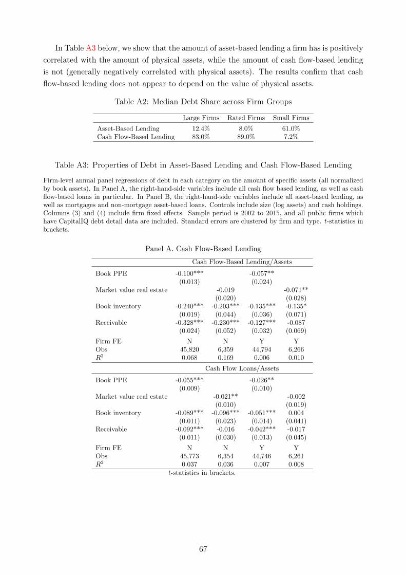
In Table A3 below, we show that the amount of asset-based lending a firm has is positively
correlated with the amount of physical assets, while the amount of cash flow-based lending
is not (generally negatively correlated with physical assets). The results confirm that cash
flow-based lending does not appear to depend on the value of physical assets.
Table A2: Median Debt Share across Firm Groups
Large Firms Rated Firms Small Firms
Asset-Based Lending 12.4% 8.0% 61.0%Cash Flow-Based Lending 83.0% 89.0% 7.2%
Table A3: Properties of Debt in Asset-Based Lending and Cash Flow-Based Lending
Firm-level annual panel regressions of debt in each category on the amount of specific assets (all normalizedby book assets). In Panel A, the right-hand-side variables include all cash flow based lending, as well as cashflow-based loans in particular. In Panel B, the right-hand-side variables include all asset-based lending, aswell as mortgages and non-mortgage asset-based loans. Controls include size (log assets) and cash holdings.Columns (3) and (4) include firm fixed effects. Sample period is 2002 to 2015, and all public firms whichhave CapitalIQ debt detail data are included. Standard errors are clustered by firm and type. t-statistics inbrackets.
Panel A. Cash Flow-Based Lending
Cash Flow-Based Lending/Assets
Book PPE -0.100*** -0.057**(0.013) (0.024)
Market value real estate -0.019 -0.071**(0.020) (0.028)
Book inventory -0.240*** -0.203*** -0.135*** -0.135*(0.019) (0.044) (0.036) (0.071)
Receivable -0.328*** -0.230*** -0.127*** -0.087(0.024) (0.052) (0.032) (0.069)
Firm FE N N Y YObs 45,820 6,359 44,794 6,266R2 0.068 0.169 0.006 0.010
Cash Flow Loans/Assets
Book PPE -0.055*** -0.026**(0.009) (0.010)
Market value real estate -0.021** -0.002(0.010) (0.019)
Book inventory -0.089*** -0.096*** -0.051*** 0.004(0.011) (0.023) (0.014) (0.041)
Receivable -0.092*** -0.016 -0.042*** -0.017(0.011) (0.030) (0.013) (0.045)
Firm FE N N Y YObs 45,773 6,354 44,746 6,261R2 0.037 0.036 0.007 0.008
t-statistics in brackets.
67
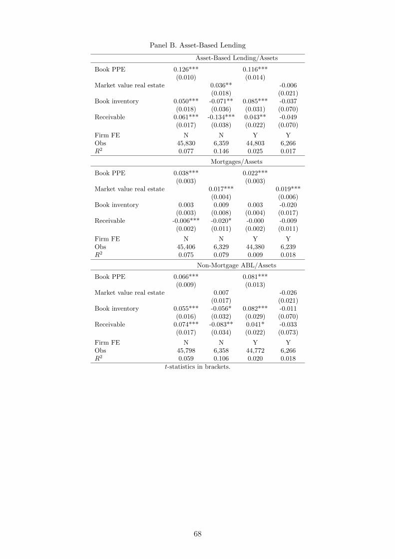
Panel B. Asset-Based Lending
Asset-Based Lending/Assets
Book PPE 0.126*** 0.116***(0.010) (0.014)
Market value real estate 0.036** -0.006(0.018) (0.021)
Book inventory 0.050*** -0.071** 0.085*** -0.037(0.018) (0.036) (0.031) (0.070)
Receivable 0.061*** -0.134*** 0.043** -0.049(0.017) (0.038) (0.022) (0.070)
Firm FE N N Y YObs 45,830 6,359 44,803 6,266R2 0.077 0.146 0.025 0.017
Mortgages/Assets
Book PPE 0.038*** 0.022***(0.003) (0.003)
Market value real estate 0.017*** 0.019***(0.004) (0.006)
Book inventory 0.003 0.009 0.003 -0.020(0.003) (0.008) (0.004) (0.017)
Receivable -0.006*** -0.020* -0.000 -0.009(0.002) (0.011) (0.002) (0.011)
Firm FE N N Y YObs 45,406 6,329 44,380 6,239R2 0.075 0.079 0.009 0.018
Non-Mortgage ABL/Assets
Book PPE 0.066*** 0.081***(0.009) (0.013)
Market value real estate 0.007 -0.026(0.017) (0.021)
Book inventory 0.055*** -0.056* 0.082*** -0.011(0.016) (0.032) (0.029) (0.070)
Receivable 0.074*** -0.083** 0.041* -0.033(0.017) (0.034) (0.022) (0.073)
Firm FE N N Y YObs 45,798 6,358 44,772 6,266R2 0.059 0.106 0.020 0.018
t-statistics in brackets.
68

CE
arn
ings-
Base
dB
orr
ow
ing
Const
rain
ts
C.1
Sp
eci
fica
tion
sof
Earn
ings-
Base
dC
oven
ant
Tab
leA
5:V
aria
nts
ofE
arnin
gs-B
ased
Cov
enan
ts
Th
ista
ble
list
sth
em
ain
vari
ants
ofea
rnin
gs-b
ased
cove
nan
tsan
dth
eco
nst
ruct
ion
usi
ng
Com
pu
stat
vari
ab
les
com
pil
edby
Dem
erji
an
an
dO
wen
s(2
016).
The
firs
tco
lum
nd
isp
lays
the
coven
ant
typ
e,w
hic
his
rep
orte
din
Dea
lSca
nd
ata
,an
dth
ese
con
dco
lum
nd
escr
ibes
the
form
of
the
coven
ant.
Th
eth
ird
colu
mn
show
sh
owto
com
pu
teth
em
etri
cu
sed
inea
chty
pe
ofco
ven
ant
usi
ng
Com
pu
stat
data
.T
he
fou
rth
colu
mn
tab
ula
tes
the
fract
ion
of
Dea
lSca
nlo
an
sto
US
non-fi
nan
cial
that
hav
eth
esp
ecifi
cty
pe
ofco
ven
ant.
Th
efi
nal
colu
mn
show
sa
chec
kof
the
Com
pu
stat
form
ula
.F
or
som
ety
pes
of
cove
nants
,th
efo
rmu
laan
dd
etail
sof
the
com
pon
ents
may
not
be
full
yst
and
ard
ized
acro
ssd
iffer
ent
deb
tco
ntr
acts
.D
emer
jian
an
dO
wen
s(2
016)
stu
dy
asu
bse
tof
Dea
lSca
nlo
an
sw
her
ed
etail
sof
the
coven
ant
form
ula
are
pro
vid
edby
the
Tea
rsh
eets
dat
aset
,an
dth
eyca
lcu
late
the
freq
uen
cyof
case
sw
her
eth
eC
om
pu
stat
form
ula
list
edis
matc
hes
wit
hd
etail
sp
rovid
edby
the
Tea
rsh
eets
dat
a.
Cov
enan
tT
yp
eS
tan
dar
dd
enit
ion
Com
pu
stat
imp
lem
enta
tion
Fra
ctio
nof
loan
sE
xact
matc
hin
Dem
erji
an
an
dO
wen
s(2
016)
Max
.D
ebt-
to-E
BIT
DA
Deb
t/E
BIT
DA
(DLT
T+
DL
C)/
EB
ITD
A29.7
%91.0
%M
ax.
Sen
ior
Deb
t-to
-EB
ITD
AS
enio
rD
ebt/
EB
ITD
A(D
LT
T+
DL
CD
S)/
EB
ITD
A5.2
%89.4
%M
in.
Inte
rest
Cov
erag
eE
BIT
DA
/Inte
rest
Exp
ense
EB
ITD
A/X
INT
20.8
%76.3
%M
in.
Cas
hIn
tere
stC
over
age
EB
ITD
A/I
nte
rest
Pai
dE
BIT
DA
/IN
TP
N0.7
%76.8
%M
in.
Deb
tS
ervic
eC
over
age
EB
ITD
A/(
Inte
rest
Exp
ense
+S
TD
ebt)
EB
ITD
A/(X
INT
+L
.DL
C)
4.5
%37.9
%M
in.
Fix
edC
har
geC
over
age
EB
ITD
A/(
Inte
rest
Exp
ense
+S
TD
ebt+
Ren
tE
xp
ense
)E
BIT
DA
/(X
INT
+L
.DL
C+
XR
EN
T)
18.5
%2.7
%M
in.
EB
ITD
AE
BIT
DA
EB
ITD
A5.0
%97.4
%
69
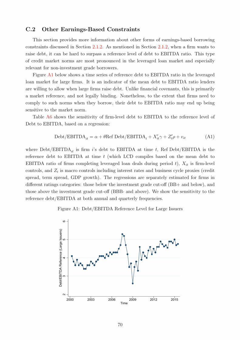
C.2 Other Earnings-Based Constraints
This section provides more information about other forms of earnings-based borrowing
constraints discussed in Section 2.1.2. As mentioned in Section 2.1.2, when a firm wants to
raise debt, it can be hard to surpass a reference level of debt to EBITDA ratio. This type
of credit market norms are most pronounced in the leveraged loan market and especially
relevant for non-investment grade borrowers.
Figure A1 below shows a time series of reference debt to EBITDA ratio in the leveraged
loan market for large firms. It is an indicator of the mean debt to EBITDA ratio lenders
are willing to allow when large firms raise debt. Unlike financial covenants, this is primarily
a market reference, and not legally binding. Nonetheless, to the extent that firms need to
comply to such norms when they borrow, their debt to EBITDA ratio may end up being
sensitive to the market norm.
Table A6 shows the sensitivity of firm-level debt to EBITDA to the reference level of
Debt to EBITDA, based on a regression:
Debt/EBITDAit = α + θRef Debt/EBITDAt +X ′itγ + Z ′tρ+ vit (A1)
where Debt/EBITDAit is firm i’s debt to EBITDA at time t, Ref Debt/EBITDA is the
reference debt to EBITDA at time t (which LCD compiles based on the mean debt to
EBITDA ratio of firms completing leveraged loan deals during period t), Xit is firm-level
controls, and Zt is macro controls including interest rates and business cycle proxies (credit
spread, term spread, GDP growth). The regressions are separately estimated for firms in
different ratings categories: those below the investment grade cut-off (BB+ and below), and
those above the investment grade cut-off (BBB- and above). We show the sensitivity to the
reference debt/EBITDA at both annual and quarterly frequencies.
Figure A1: Debt/EBITDA Reference Level for Large Issuers
23
45
6D
ebt/E
BITD
A R
efer
ence
(Lar
ge Is
suer
s)
2000 2003 2006 2009 2012 2015Time
70
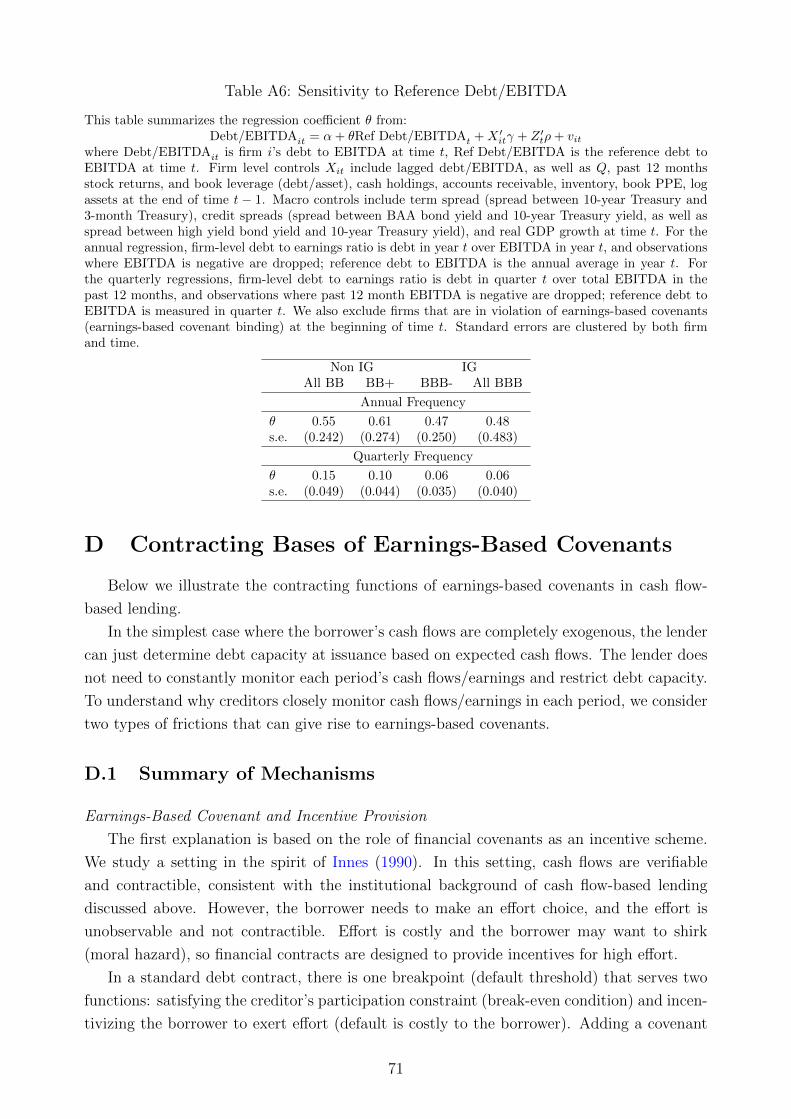
Table A6: Sensitivity to Reference Debt/EBITDA
This table summarizes the regression coefficient θ from:Debt/EBITDAit = α+ θRef Debt/EBITDAt +X ′itγ + Z ′tρ+ vit
where Debt/EBITDAit is firm i’s debt to EBITDA at time t, Ref Debt/EBITDA is the reference debt toEBITDA at time t. Firm level controls Xit include lagged debt/EBITDA, as well as Q, past 12 monthsstock returns, and book leverage (debt/asset), cash holdings, accounts receivable, inventory, book PPE, logassets at the end of time t − 1. Macro controls include term spread (spread between 10-year Treasury and3-month Treasury), credit spreads (spread between BAA bond yield and 10-year Treasury yield, as well asspread between high yield bond yield and 10-year Treasury yield), and real GDP growth at time t. For theannual regression, firm-level debt to earnings ratio is debt in year t over EBITDA in year t, and observationswhere EBITDA is negative are dropped; reference debt to EBITDA is the annual average in year t. Forthe quarterly regressions, firm-level debt to earnings ratio is debt in quarter t over total EBITDA in thepast 12 months, and observations where past 12 month EBITDA is negative are dropped; reference debt toEBITDA is measured in quarter t. We also exclude firms that are in violation of earnings-based covenants(earnings-based covenant binding) at the beginning of time t. Standard errors are clustered by both firmand time.
Non IG IGAll BB BB+ BBB- All BBB
Annual Frequency
θ 0.55 0.61 0.47 0.48s.e. (0.242) (0.274) (0.250) (0.483)
Quarterly Frequency
θ 0.15 0.10 0.06 0.06s.e. (0.049) (0.044) (0.035) (0.040)
D Contracting Bases of Earnings-Based Covenants
Below we illustrate the contracting functions of earnings-based covenants in cash flow-
based lending.
In the simplest case where the borrower’s cash flows are completely exogenous, the lender
can just determine debt capacity at issuance based on expected cash flows. The lender does
not need to constantly monitor each period’s cash flows/earnings and restrict debt capacity.
To understand why creditors closely monitor cash flows/earnings in each period, we consider
two types of frictions that can give rise to earnings-based covenants.
D.1 Summary of Mechanisms
Earnings-Based Covenant and Incentive Provision
The first explanation is based on the role of financial covenants as an incentive scheme.
We study a setting in the spirit of Innes (1990). In this setting, cash flows are verifiable
and contractible, consistent with the institutional background of cash flow-based lending
discussed above. However, the borrower needs to make an effort choice, and the effort is
unobservable and not contractible. Effort is costly and the borrower may want to shirk
(moral hazard), so financial contracts are designed to provide incentives for high effort.
In a standard debt contract, there is one breakpoint (default threshold) that serves two
functions: satisfying the creditor’s participation constraint (break-even condition) and incen-
tivizing the borrower to exert effort (default is costly to the borrower). Adding a covenant
71
allows the creditor to specify a separate threshold, covenant violation, for incentive provision.
Covenant violation imposes costs to the borrower, such as punishment fees or significant non-
monetary costs (time spent dealing with creditors, restrictions on corporate policies, man-
agement being replaced, etc.), and incentivizes the borrower to work hard to avoid violation.
By allowing the contract to decouple the incentive effect from the breakeven condition, the
covenant can decrease the cost of incentivizing the borrower (helps satisfy the borrower’s
incentive compatibility constraint). The formal model is shown below in Appendix D.2.
Earnings-Based Covenant as Contingent Transfer of Control Rights
The second explanation views covenant violation as a signal that default on debt pay-
ment may become possible, and the creditor should consider stepping in to take actions.
Specifically, when earnings are above the threshold specified by the covenant, default is re-
mote; creditors can rest assured and do not need to pay much attention. When earnings
fall below the covenant threshold, there are warning signs that the borrower’s ability to pay
back the debt could be in question and creditors may suffer losses. In this case, creditors
may want to step in and take some otherwise costly actions to improve firm performance.
Because creditors enjoy most of the benefits from such actions (such actions only improve
firm performance in bad states), the borrower/firm shareholders cannot commit to it. As a
result, financial covenants are placed in debt contracts as an early warning sign, and they
can trigger partial transfers of control rights to creditors. This view builds along the idea
of contingent control rights (Aghion and Bolton, 1992) and the evidence on control right
transfers following covenant violations (Chava and Roberts, 2008; Roberts and Sufi, 2009).
The formal model is shown below in Appendix D.3.
Why Covenants based on Earnings/EBITDA?
Finally, we discuss why financial covenants in cash flow-based lending emphasize current
earnings as a key metric to serve the contracting functions discussed above (incentive pro-
vision or contingent transfer of control rights). The evaluation metric needs to have several
properties. First, it needs to be informative about firm performance, which is central to both
of the rationales we considered. Firm performance shows the manager’s effort. It also signals
the necessity for creditor interventions (the borrower’s financial performance/cash flow value
is especially important to creditor payoffs in cash flow-based lending). Second, the metric
needs to be easy to observe and measure, so that it can be assessed on a frequent basis, and
borrowers and lenders do not dispute its value.
In the US, with an accounting system that is reliable and well-designed to reflect the
economic activities of the firm, earnings are informative and serve as a central measure of
performance. Moreover, among various possible measures of earnings, creditors place most
weight on EBITDA to reflect the performance and cash flow generation ability of the firm’s
core business. Financial covenants also focus on current/recent earnings which are readily
observable based on financial statements, rather than future earnings which are unobservable
and not easily contractible.42
42One may wonder whether financial covenants can use other measures. We discuss several alternatives
72
D.2 Model 1: Incentive Provision
Below we provide a model that illustrates the role of financial covenants for incentive
provision.
The model has two stages, t = 1, 2. In stage t = 1, the risk neutral borrower needs to
borrow B > 0 dollars from the risk neutral creditor to continue operations. If operations
continue, the borrower needs to make an unobservable effort choice, e ∈{eL, eH
}, generating
cost g (e) to the borrower. In stage t = 2, the borrower generates observable and verifiable
earnings/cash flows R with p.d.f. fe (R) and c.d.f. Fe (R), where e ∈{eL, eH
}, and needs to
repay debt obligations. We assume a competitive lending market, so the optimal contract
maximizes the borrower’s payoff, subject to the creditor’s participation constraint (IR-C) and
the borrower’s incentive compatibility constraint of not shirking (IC-B).43 For simplicity, we
assume the gross interest rate to be 1.
We focus on whether adding an earnings-based covenants to an otherwise standard debt
contract44 can improve the borrower’s payoff. The face value of debt is denoted by D > 0.
On top of it, an earnings-based covenants with threshold C ≥ D can be added. When the
covenant is violated, the borrower faces a “technical default,” and bears a non-monetary cost
of A > 0 (which may come from creditor interventions, time costs of dealing with creditors,
career costs, etc.). When C = D, the contract degenerates to a standard debt contract, and
the borrower only incurs the non-monetary cost if he misses debt payment.45
In this environment, the optimal debt contract (with covenants) solves the following
and why they are not applied in cash flow-based lending. First, relative to earnings, the value of physicalassets can be driven by many factors and is less informative about the borrower’s performance. It can also bedifficult to measure on a frequent basis, especially when assets are specialized and illiquid. Second, statisticalmeasures of distance/probability to default can be relevant, but they are difficult to assess. Debtors andcreditors can dispute about the computation, making it harder to contract on. Finally, financial covenantsalso do not use metrics such as stock prices, which can fluctuate due to non-fundamental reasons. In addition,investors can deliberately influence stock prices to trigger or avoid covenant violations, which can significantlycomplicate the situation.
43We assume the cost of not continuing operations to the borrower is very high, so the borrower’s partic-ipation constraint always holds.
44Innes (1990) shows that a debt-like contract is optimal in this environment, as it provides best incentivesfor the borrower to work. That is why we focus on debt contracts here. We discuss the relationship with theparticular contract Innes (1990) considered in footnote 47.
45For simplicity, in the current environment, the non-monetary cost A to the borrower when the covenantis violated (i.e. D ≤ R < C) and such cost when the borrower misses debt payment (i.e. R < D) is thesame. The key result, Proposition A1, extends to settings where the non-monetary costs at these two eventsare different. Moreover, Proposition A1 also holds when there is additional monetary cost of the paymentdefault (e.g. monetary cost associated with bankruptcy).
73

constrained maximization problem:
U∗ = supC,D
∫ (max {R−D, 0} − A1{R<C}
)feH (R) dR− g
(eH)≡ sup
C,DUB (C,D) , (A2)
s.t. IC −B :
∫ (max {R−D, 0} − A1{R<C}
)feH (R) dR− g
(eH)≥∫ (
max {R−D, 0} − A1{R<C})feL (R) dR− g
(eL), (A3)
IR− C :
∫min {R,D} feH (R) dR ≥ B, (A4)
C ≥ D, (A5)
Condition (A2) specifies the payoff to the borrower. It consists of three components. First,
max {R−D, 0} is the monetary payoff to the borrower when the realized earnings/cash flows
is R. Second, the borrower incurs a non-monetary cost A when the covenant is violated or
debt payment is missed. Third, the borrower incurs a cost of g(eH)
by exerting high efforts.
Condition (A3) specifies the borrower’s incentive compatibility constraint of not shirking
(IC-B): the borrower’s utility is higher under eH than eL.46 Condition (A4) specifies the
expected payoff to the creditor is weakly higher than the amount lent to the borrower, B,
so the creditor has incentive to participate (IC-R). Condition (A5) requires the covenant
violation cutoff to to be weakly higher than the debt face value/payment default threshold.
Under the standard debt contract, C = D: the incentive effects provided by the non-
monetary costs are determined by the face value of debt D (under the standard debt contract,
the utility difference between high and low levels of effort, which comes from from the non-
monetary cost, is∫−A1{R<D}feH (R) dR−
(∫−A1{R<D}feL (R) dR
)= A (FeH (D)− FeL (D))).
Adding an earnings-based covenant, C > D, allows the contract to decouple debt payment,
D, and incentive effects (the utility difference between high and low efforts coming from
the non-monetary cost is now given by∫−A1{R<C}feH (R) dR−
(∫−A1{R<C}feL (R) dR
)=
A (FeH (C)− FeL (C))). The introduction of earnings based covenants helps to provide more
effective incentives for the borrower to exert high effort, and helps to achieve the constrained
optimum. We formalize this intuition in Proposition A1.47 We state a few standard (techni-
cal) assumptions first.
46This raises the question of why the optimal contract wants to implement high effort eH , instead ofshirking eL. We assume
∫RfeL (R) dR < B. As a result, the expected payoff generated by shirking is
not enough to compensate the creditor. A contract implementing eL cannot satisfy creditor’s participationconstraint.
47Innes (1990) considers two types of contracts: a “live or die” contract and a standard debt contract.The “live or die” contract features a discrete jump in the borrower’s payoff if he does not default on debtpayment, similar to the effect of A > 0 here. This is the optimal contract without any restriction on thecontract space. However, a contract with discrete jumps may create incentives for the borrower to get a fewextra dollars and avoid the jump. The debt contract Innes (1990) considers avoids such the discrete jumpof the borrower’s payoff (this requires A = 0 in our notation), and provides a smooth payoff scheme. In ourview, as widely documented in the empirical literature on debt covenants, the event of covenant violationindeed incurs significant costs to the borrower, and borrowers try to avoid such violations. However, thiscost should not be a free variable that can be chosen by the contract as in the “live or death” contract. Asa result, we choose a fixed cost A > 0 and explores its implications for optimal contract design.
74

Assumption A1 (Full and Non-Moving Support). The p.d.f of R satisfies:
feL (R) , feH (R) > 0, ∀R ∈ [Rmin, Rmax] ;
feL (R) = feH (R) = 0, ∀R 6/∈ [Rmin, Rmax] .
Assumption A2 (Monotone Likelihood Ratio Property (MLRP)). The likelihood ratio
L (R) =feH
(R)
feL
(R)is increasing in R ∈ [Rmin, Rmax] .
Assumptions A1 and A2 are standard regularity assumptions to make the problem well
behaved. By Assumption A2, there exists R, such thatL (R) =feH
(R)
feL
(R)< 1 R < R
L (R) =feH
(R)
feL
(R)≥ 1 R ≥ R.
Now we state the assumption under which at least one contract will satisfy the constraints
in conditions (A3), (A4) and (A5), so the problem in (A2) is well defined.
Assumption A3. [Existence]
i) Under high efforts, the borrower generates enough output to repay the creditor:∫RfeH (R) dR > B.
As a result, there exists a D ∈ [0, Rmax) that uniquely pins down the creditor’s break-even
condition, ∫min
{R, D
}feH (R) dR = B, (A6)
thus condition (A4) holds with equality.
ii) Under contract (C,D) =(max
{D, R
}, D), the borrower’s IC condition gets satis-
fied:48 ∫ (max
{R− D, 0
}− A1{R<max{D,R}}
)feH (R) dR− g
(eH)≥∫ (
max{R− D, 0
}− A1{R<max{D,R}}
)feL (R) dR− g
(eL). (A7)
We will now be able to formalize the previous intuition about why earnings based covenant
is helpful, and state Proposition A1.The proof is provided in the Internet Appendix.
Proposition A1. Under Assumptions A1, A2 and A3, we establish:
(i) The set of contracts that satisfy all of the constraints (A3) - (A5) are non-empty.
Moreover, there exists a contract (C∗, D∗) that achieves the supremum U∗ defined in condition
(A2).
48In fact, we can prove that, if condition (A7) is violated, the borrower’s IC condition is not satisfiedunder any contract. In this sense, contract (C,D) =
(max
{D, R
}, D)
is the “best” contract in terms ofhelping to achieve the borrower’s IC constraint.
75
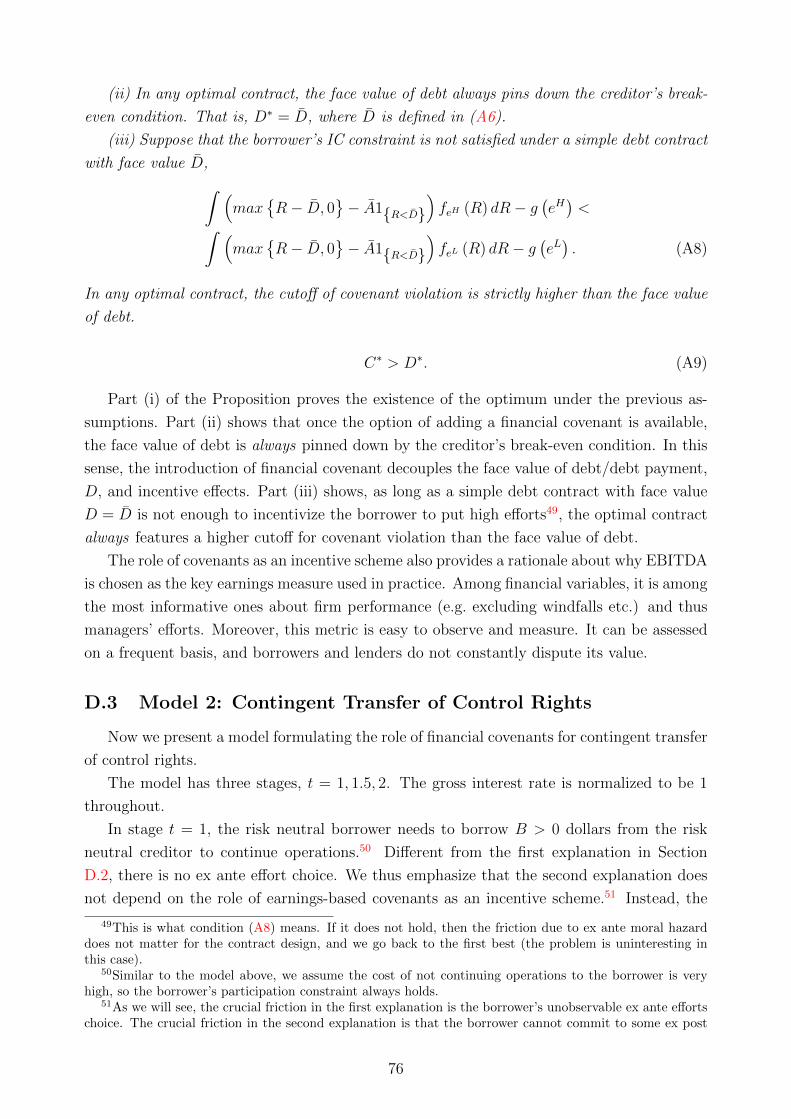
(ii) In any optimal contract, the face value of debt always pins down the creditor’s break-
even condition. That is, D∗ = D, where D is defined in (A6).
(iii) Suppose that the borrower’s IC constraint is not satisfied under a simple debt contract
with face value D,∫ (max
{R− D, 0
}− A1{R<D}
)feH (R) dR− g
(eH)<∫ (
max{R− D, 0
}− A1{R<D}
)feL (R) dR− g
(eL). (A8)
In any optimal contract, the cutoff of covenant violation is strictly higher than the face value
of debt.
C∗ > D∗. (A9)
Part (i) of the Proposition proves the existence of the optimum under the previous as-
sumptions. Part (ii) shows that once the option of adding a financial covenant is available,
the face value of debt is always pinned down by the creditor’s break-even condition. In this
sense, the introduction of financial covenant decouples the face value of debt/debt payment,
D, and incentive effects. Part (iii) shows, as long as a simple debt contract with face value
D = D is not enough to incentivize the borrower to put high efforts49, the optimal contract
always features a higher cutoff for covenant violation than the face value of debt.
The role of covenants as an incentive scheme also provides a rationale about why EBITDA
is chosen as the key earnings measure used in practice. Among financial variables, it is among
the most informative ones about firm performance (e.g. excluding windfalls etc.) and thus
managers’ efforts. Moreover, this metric is easy to observe and measure. It can be assessed
on a frequent basis, and borrowers and lenders do not constantly dispute its value.
D.3 Model 2: Contingent Transfer of Control Rights
Now we present a model formulating the role of financial covenants for contingent transfer
of control rights.
The model has three stages, t = 1, 1.5, 2. The gross interest rate is normalized to be 1
throughout.
In stage t = 1, the risk neutral borrower needs to borrow B > 0 dollars from the risk
neutral creditor to continue operations.50 Different from the first explanation in Section
D.2, there is no ex ante effort choice. We thus emphasize that the second explanation does
not depend on the role of earnings-based covenants as an incentive scheme.51 Instead, the
49This is what condition (A8) means. If it does not hold, then the friction due to ex ante moral hazarddoes not matter for the contract design, and we go back to the first best (the problem is uninteresting inthis case).
50Similar to the model above, we assume the cost of not continuing operations to the borrower is veryhigh, so the borrower’s participation constraint always holds.
51As we will see, the crucial friction in the first explanation is the borrower’s unobservable ex ante effortschoice. The crucial friction in the second explanation is that the borrower cannot commit to some ex post
76

earnings/cash flows generated at stage t = 2, R (x), is a function of the exogenous state
of the world, x ∈ [xmin, xmax], in stage 2. Without loss of generality, we assumes R (x) is
increasing in x.52
In the intermediate stage t = 1.5, an observable state of nature s ∈ [smin, smax] is revealed,
which serves as a “signal” about x. When s is low (high), it means low (high) x is more
likely. In particular, let Fs (x) denote the distribution (c.d.f.) of x conditional on s. We
assume, if s > s′,
Fs (x) first order stochastic dominates Fs′ (x) . (A10)
As a result,
E [R (x) |s] is increasing in s.
In this intermediate stage, an additional action can be taken, which generates additional
observable and verifiable earnings/cash flows Y (x) in stage t = 2. Such actions are only
efficient when x is bad. In particular, Y (x) is decreasing in x (We still maintain that
Y (x) +R (x) is increasing in x.) Moreover, there is an cutoff x ∈ (xmin, xmax), such thatY (x) > 0 if x < x
Y (x) ≤ 0 if x ≥ x. (A11)
Such an action can be thought as an “emergency plan” that is otherwise costly in the good
states of the world.
In stage t = 2, the state of nature x, is revealed, and the borrower generates observable
and verifiable earnings/cash flows R (x). If the “emergency plan” project is taken, an addi-
tional observable and verifiable earnings/cash flows Y (x) is generated. The borrower needs
to repay his debt obligations, with face value D, in stage 2. As before, we assume a com-
petitive lending market, so the optimal contract maximizes the borrower’s payoff, subject to
the creditor’s participation constraint (IR-C).
Let us first consider the first best, where the “emergency plan” project is taken if and
only if s ≤ s, where s is the cutoff such that53E [Y (x) |s] > 0 if s < s
E [Y (x) |s] ≤ 0 if s ≥ s.
Under first best, the creditor’s realized payoff is min {D,R (x) + Y (x) 1s<s}. To satisfy the
creditor’s participation constraint (IR), it must be the case that E [min {D,R (x) + Y (x) 1s<s}] ≥B. A competitive lending market then pins down D = D∗ by letting the previous condition
hold with equality. The borrower’s realized utility is then given by max {R (x) + Y (x) 1s<s −D∗, 0}.How can the first best can be implemented? A standard debt contract in which the
borrower always has control rights in the intermediate stage t = 1.5 may not do the job.
actions that are beneficial in the bad states.52We also assume E [R (x)] > B, so there is enough output to compensate the borrower.53The existence of such cutoff comes from conditions (A10) and (A11).
77

This is because the “emergency plan” is beneficial in bad states of the world, but is otherwise
costly in good states of the world; the creditor enjoys the majority of benefits from such an
action, and the borrower may not be able to commit to implementing it even when s is
revealed revealed in the intermediate stage.54 For example, we have:
Proposition A2. Assume R (xmin) ≤ D ≤ R (xmax), so there exists a unique xD such that
R (xD) = D.55 As long as Y (xD) ≤ 0, for all s,
E [max {R (x) + Y (x)−D, 0} |s] ≤ E [max {R (x)−D, 0} |s] . (A12)
Moreover, if for a given s, there is a positive measure of x under Fs such that
max {R (x) + Y (x)−D, 0} < max {R (x)−D, 0} ,
The condition Y (xD) ≤ 0 means that, in the state of world where the borrower starts
to receive payment, the “emergency plan” project is already inefficient.56 In this case, the
borrower weakly prefers not to implement the “emergency plan” in any state of the world
in the intermediate stage. Moreover, if for a given intermediate state s, there is a positive
measure of final states x such that taking the “emergency plan” project is strictly worse off
for the borrower, then the borrower will strictly prefer not to implement such “emergency
plan” in state s. This explains why the optimal contract needs to feature a covenant that
transfers the control rights to the creditor in certain states of the world.
Now we show that a financial contract specifying a contingent transfer of control rights
from the borrower to the creditor when s < s in the intermediate state can implement the
first best. To be concrete, we have:57
Proposition A3. For all D > 0 and s < s,
E [min {D,R (x) + Y (x)} |s] ≥ E [min {D,R (x)} |s] . (A13)
This means the creditor always has incentives to implement the “emergency plan” when
s < s. As a result, the first best can be implemented by a standard debt contract with face
value D∗ and a covenant transferring the control rights to the creditor when s < s.
As EBITDA is among the most informative financial variables about firm performance, it
can serve as a helpful signal. In addition, this metric is easy to observe and measure, and can
be assessed on a frequent basis. Accordingly, one can write a covenant that transfers control
rights when EBITDA is too low, approximating the transfer of control rights in state s < s
54Such frictions is akin to frictions studied in the “debt overhang” literature (Myers, 1977).55Note that any debt face value D ≥ R (xmax) is equivalent to D = R (xmax) in terms of payoffs, as
Y (xmax) < 0. So assume D ≤ R (xmax) is without loss of generality.56Note that this does not mean there does not exist state s in the intermediate stage such that the
“emergency plan” is efficient for s ≤ s.57The proposition can also be extended to the case with costs of bankruptcy, but such costs are not
required.
78

modeled in Proposition A3. Thus, earnings-based covenants can be thought as a mechanism
for contingent transfers of control rights.
E Classic Models of Corporate Borrowing
In this appendix, we further discuss several strands of literature on costly external financ-
ing and their predictions about how cash flows influence corporate borrowing and investment.
We clarify the differences between predictions based on EBCs and predictions in these mod-
els. As discussed in Section 3.1, in these other models, cash flows only affect corporate
borrowing through the impact on internal funds; EBITDA does not have an independent
role after controlling for internal funds. We summarize the detailed predictions below.
1. This paper
• Determinant of cost/capacity for external borrowing: Operating earnings.
• Formulation: C (b, π); π is operating earnings (EBITDA).
• How cash flows influence borrowing and investment: Cash flows in the form of
EBITDA relax borrowing constraints/decrease cost of external borrowing, and
crowd in borrowing and investment. Holding EBITDA constant, cash receipts
increase internal funds, but do not relax borrowing constraints/decrease cost of
external borrowing. They boost investment but substitute out external borrowing.
• EBITDA plays an independent role controlling for internal funds.
2. Froot, Scharfstein, and Stein (1993), Kaplan and Zingales (1997)
• Determinant of cost/capacity for external borrowing: Exogenous (not dependent
on financial variables).
• Formulation: C(b).
• How cash flows influence borrowing and investment: Cash flows increase internal
funds, but do not relax borrowing constraints/decrease cost of external borrowing.
They boost investment but substitute out external borrowing.
• EBITDA does not play an independent role controlling for internal funds.
3. Kiyotaki and Moore (1997), Bernanke, Gertler, and Gilchrist (1999)
• Determinant of cost/capacity for external borrowing: Liquidation value of physical
assets.
• Formulation: C(b, qk). k is the amount of physical capital the firm owns, q is the
liquidation value per unit of capital measured at the time of debt repayment.
79

• How cash flows influence borrowing and investment: Borrowing constraints/cost
of external borrowing do not directly depend on cash flows. Higher cash flows
may increase borrowing indirectly as they increase firms’ internal funds (“net
worth”), allow firms to acquire more physical assets, and relax firms’ borrowing
constraints/decreases cost of external financing.
• EBITDA does not play an independent role controlling for internal funds.
4. Holmstrom and Tirole (1997)
• Determinant of cost/capacity for external borrowing: Pledgeable income.
• Formulation: C(b, P ). P is the amount of pledgeable income a firm has.
• How cash flows influence borrowing and investment: Borrowing constraints/cost
of external borrowing do not directly depend on cash flows. Higher cash flows
may increase borrowing indirectly as they increase firms’ internal funds (“net
worth”), allow firms to acquire more projects, and therefore generate more pledge-
able income and relax firms’ borrowing constraints/decreases its cost of external
financing.
• EBITDA does not play an independent role controlling for internal funds.
The concept “net worth channel” is used in both the third case and the fourth case.
“Net worth” is defined as the firm’s maximum amount of funds available that can be used to
acquire new assets and projects (Bernanke, Gertler, and Gilchrist, 1999). This is equivalent
to internal funds w in our framework.
In the case of Kiyotaki and Moore (1997) and Bernanke, Gertler, and Gilchrist (1999),
the net worth channel means that an increase in internal funds w allows firms to acquire
more physical assets and relax its borrowing constraints, as discussed above. In the case of
Holmstrom and Tirole (1997), the net worth channel then means that an increase in internal
funds w allows firms to acquire more projects, generate more pledgeable income and relax its
borrowing constraints, as discussed above. Taken together, the net worth channel captures
how internal funds influence borrowing; EBITDA does not play an independent role after
controlling for internal funds in this case.
F Accounting
F.1 EBITDA and OCF
Definition and Construction
1. EBITDA
• Compustat variable: EBITDA (equivalently OIBDP)
80

• EBITDA is a measure of operating earnings
• EBITDA = revenue - operating expenses = sales (SALE) - cost of goods sold
(COGS) - selling, general and administrative expense (XSGA)
• Does not include capital expenditures (CAPX), which is separately accounted as
cash flows from investment activities. Does include R&D expenses, which count
towards operating expenses (included in COGS and XSGA); R&D spending is
required to be immediately expensed.
2. OCF
• Compustat variable: OANCF + XINT
– XINT: Interest Expenses. The Compustat variable OANCF subtracts interest
expenses. We add them back to avoid mechanical correlations with debt
issuance.
• OCF is a measure of the net cash receipts (inflows minus outflows) a firm gets from
operating activities (as opposed to investing activities or financing activities).
• OCF is typically calculated via the indirect method, i.e. starting with earnings
and add back/subtract non-cash components. Based on Compustat variable def-
initions, the following relation holds:
OCF = EBITDA +(NOPI + SPI) + SPPE︸ ︷︷ ︸non-operating & other income
−(TAX−DTAX−∆ATAX)︸ ︷︷ ︸cash taxes paid
+∆AP−∆AR−∆INV︸ ︷︷ ︸∆NWC
+ ∆UR−∆PX︸ ︷︷ ︸cash income/costnot in earnings
+OCFO (A14)
– NOPI: Nonoperating Income (e.g. dividend, interest, rental, royalty income).
– SPI: Special Item (e.g. windfalls, natural disaster damages, earnings from
discontinued operations, litigation reserves). Based on the Compustat defini-
tion, variables XIDOC (cash flows from extraordinary items & discontinued
operations) and MII (noncontrolling interest) are also added back.
– SPPE: Sale of Property, Plant and Equipment.
– TXT: Total Income Taxes; TXD: Deferred Taxes; ∆TXA: Changes in Ac-
crued Taxes. TXT− TXD−∆TXA is cash payment of taxes.
– ∆AP: Changes in Accounts Payable.
– ∆AR: Changes in Accounts Receivable.
– ∆INV: Changes in Inventory.
– ∆UR: Changes in unearned revenue. For instance, if a firm receives cash for
purchases of goods and services to be delivered in the future (e.g. membership,
subscription, gift card), it does not record any earnings but gets more cash.
This leads to an increase in unearned revenue. ∆UR: Changes in prepaid
81

expenses. Similarly, if a firm pays for goods or services to be delivered to it
in the future (e.g. insurance), it does not record an expense but has less cash.
This leads to an increase in prepaid expenses. OCFO: other miscellaneous
cash flows from operations. See Compustat definitions of OANCF.
• Does not include capital expenditures (CAPX), which is separately accounted in
cash flows from investment activities. Does include R&D expenses, which count
towards operating expenses (included in COGS and XSGA); R&D spending is
required to be immediately expensed. Does not include the effect of payouts and
securities issuance, which are separately accounted in cash flows from financing
activities.
3. Difference between EBITDA and OCF
• There are two main differences between the EBITDA and OCF variables.
First, OCF takes into account the cash receipts due to non-operating income,
asset sales, windfalls, minority interests, etc., which are items not included in
EBITDA.
Second, due to accounting principles, earnings recognition and cash payments may
not happen concurrently. Cash payments may occur before, at the same time, or
after earnings recognition. For instance, it is customary for companies to make
sales and receive payments from customers later. Companies may also receive
payments first before delivering goods and services (e.g. customers purchase gift
cards and only use them later, or customers purchase membership/subscription
that they use later).
Discussion
In the baseline regression of Section 3.2, we first have a specification where the right hand
side is EBITDA (with other controls but no OCF). Variations in EBITDA come from sales
and operating expenses: EBITDA is high either because sales are high or because expenses
are low. When EBITDA is high, the firm may also receive more cash. Suppose firm A has
EBITDA 20 and firm B has EBITDA 10. With EBC, firm A’s debt capacity expands more
than firm B, helping firm A to borrow more and investment more. But firm A may also
receive more cash than firm B: more cash may lead to less borrowing and more investment
spending (using the cash) based on the traditional mechanisms in Froot, Scharfstein, and
Stein (1993). Accordingly, the positive comovement between EBITDA and cash receipts may
push the EBITDA coefficient downward when the outcome variable is debt issuance; it may
push the EBITDA coefficient upward when the outcome variable is investment.
Thus we then use a specification where the right hand side includes EBITDA, and we
also control for OCF to take into account the impact of literal cash receipts on debt is-
suance/investment. Given that EBITDA and OCF are related (as shown by Equation (A14),
below we discuss how to understand variations in each of the two variables.
82
1. Coefficient on EBITDA
• Based on the definition of EBITDA discussed above, variations in EBITDA come
from either sales or operating expenses. Whether cash associated with sales/expenses
comes in advance, concurrently, or later does not affect EBITDA.
• If two firms end up with same OCF, but have different EBITDA, there will be
accompanying differences in the second to last terms of Equation (A14). But they
do not cause differences in EBITDA.
– For example, consider firm A with EBITDA 20, NOPI 0, and OCF 20, and
firm B with EBITDA 10, NOPI 10, and OCF 20. They happen to have the
same OCF and different EBIDA because they have different NOPI. The dif-
ferent NOPI does not cause differences in EBITDA, because by the definition
of EBITDA, it is not affected by NOPI.
– For another example, consider firm A with EBITDA 20 and firm B with
EBITDA 10. Firm B happens to receive payments of 10 from customers for
previous purchases. In this case, both firms have OCF 20: firm A has more
EBITDA and firm B has some idiosyncratic cash receipts to get the same
OCF despite lower EBITDA.
• One question is whether some components of the second to last terms of Equa-
tion (A14) may themselves cause variations in debt issuance/investment. In the
example above, for two firms with the same OCF, would lower NOPI be a driver
of higher debt issuance/investment?
This type of issue does not seem obvious for NOPI. It could be more relevant in
a few cases, which we discuss below.
We first consider changes in accounts receivable ∆AR. Suppose firm A has
EBITDA 20, ∆AR 0 (all the earnings are concurrently received in cash), and
OCF 20, while firm B has EBITDA 30, ∆AR 10 (20 of the EBITDA is received
in cash, while 10 is booked as receivable), and OCF 20. One concern is firm B
expects to receive 10 in the next period, and it could pledge the receivable as
collateral to borrow more. Even in the absence of EBCs, if firms borrow by pledg-
ing receivable, we may see firm B borrow more than firm A.58 Such borrowing
based on receivable is more likely to be short term, so we focus on the issuance
of long-term debt. In addition, such borrowing is also secured debt, while our
results also hold among unsecured debt.
Another case worth considering is changes in inventory. Changes in inventory
∆INV has several components: ∆INV = (INVPt+1t +INVPt
t)−(INVPtt+INVPt
t−1).
58This issue with accounts receivable could exist even when we do not control for OCF. Consider a limitingcase where all sales are paid by receivable rather then cash. Then variations in sales are entirely variationsin receivable.
83

– INVPt+1t denotes inventory purchased in period t for future production. It
counts toward OCF in period t but does not affect EBITDA in period t.
– INVPtt denotes inventory purchased in period t for period t production. It
affects both EBITDA and OCF by the same amount in period t.
– INVPtt−1 denotes inventory purchased before period t use in period t produc-
tion. It affects the EBITDA of period t (counts toward cost of goods sold in
period t, but does not affect OCF in period t.
– The sum INVPt+1t + INVPt
t is inventory purchase in period t. The sum
INVPtt + INVPt
t−1 is reported as cost of goods sold in period t (a compo-
nent of EBITDA).
As shown above, changes in the inventory balance can come from two sources:
1) usage of old inventory, and 2) purchase of inventory for future production.
There are two corresponding situations to consider. The first situation focuses
on usage of old inventory. Suppose firm A makes sales of 30, which uses old
inventory (INVPtt−1) 10, and it purchases additional inventory of 10 for future
production (INVPt+1t ). Accordingly, firm A has EBITDA 20, OCF 20, and ∆INV
0. Firm B makes sales of 30, which used old inventory (INVPtt−1) 20, and it
purchases additional inventory of 10 for future production (INVPt+1t ). So firm B
has EBITDA 10, OCF 20, and ∆INV -10. In this situation, firm A and firm B
have the same OCF and different EBITDA. The difference in EBITDA is driven
by the fact that firm A produced the same amount of goods using less (old)
material. This variation in EBITDA is fine, except we need to be careful about
the investment opportunity issue which was addressed extensively in Section 3.2.
The second situation focuses on purchases of new inventory. Suppose firm A makes
sales of 30, which uses old inventory (INVPtt−1) 10, and it purchases additional
inventory of 20 for future production (INVPt+1t ). Accordingly, it has EBITDA
20, OCF 10, and ∆INV 10. Firm B makes sales of 20, which uses old inventory
(INVPtt−1) 10, and it purchases additional inventory of 10 for future production
(INVPt+1t ). Thus firm B has EBITDA 10, OCF 10, and ∆INV 0. Now firm A
and firm B have the same OCF, different EBITDA, and firm A purchased more
inventory. To the extent that investment opportunities are well measured, inven-
tory purchase would not add additional information about investment decisions.
As we discuss below, inventory purchase is more likely to affect the OCF coeffi-
cient, so in the Internet Appendix Table IA2, we also provide results controlling
for inventory purchase.
2. Coefficient on OCF
• As shown by Equation (A14), if two firms have the same EBITDA but different
OCF, it would be due to the second term to the last term.
84

– For example, suppose firm A and firm B both have EBITDA 20, while firm
A has NOPI 10 and firm B has NOPI 0, then firm A will have OCF 30 and
firm B will have OCF 20.
– For another example, suppose firm A and firm B both have EBITDA 20,
while firm A happens to receive payments of 10 from customers for previous
purchases. In this case, firm A has OCF 30 and firm B has OCF 20; firm A
has gets more OCF due to idiosyncratic cash receipts.
• In both of the above cases, firm A gets more internal funds at its disposal. It
may borrow less or invest more (using these internal funds), which reflect the
mechanism of Froot, Scharfstein, and Stein (1993). This would lead to a negative
coefficient on OCF when the outcome variable is debt issuance, and a positive
coefficient on OCF when the outcome variable is investment, as predicted by
Froot, Scharfstein, and Stein (1993).
• There are several cases where we need to be more careful about movements in
OCF, which we discuss below.
First, consider a case about accounts receivable: suppose firm A and firm B have
the same EBITDA, and firm A receives cash while firm B gets receivables. In
this situation, firm A gets more internal resources than firm B. Firm A may
use the internal resources and borrow less than firm B, as predicted by Froot,
Scharfstein, and Stein (1993). A caveat is firm B, which has less OCF, may pledge
its receivables as collateral to borrow more. This can attenuate the predictions
of Froot, Scharfstein, and Stein (1993). As discussed above, we focus on long-
term debt and also study unsecured debt to minimize potential issues related to
receivables.
Second, consider a case about accounts payable: suppose firm A and firm B have
the same EBITDA, but firm A decides to pay its suppliers more slowly. In this
case, firm A will have an increase in ∆AP as well as more OCF. Effectively firm
A is borrowing from suppliers; it now has more internal cash and may raise less
money from capital markets. To the extent that borrowing from suppliers is less
costly than external financing in capital markets, stretching accounts payable is
one way of generating internal funds and using them as substitutes for external
financing. This is consistent with the mechanism of Froot, Scharfstein, and Stein
(1993).
Finally, consider a case related to inventory purchases: suppose firm A and firm B
have the same EBITDA, but firm A purchases more inventory for future produc-
tion (INVPt+1t ), then firm A will have lower OCF. These purchases of inventories
may require more external financing and are associated with more debt issuance.
Thus we also present results controlling for inventory purchases.
85

F.2 Earnings Management
In the baseline regressions in Section 3.2, one driver of variations in EBITDA could
be earnings management. For example, when EBCs become binding, firms may recognize
earnings more aggressively (e.g. under-estimate operating expenses, or over-estimate sales
or accounts receivable) so they can keep more debt. The survey of managers by Graham,
Harvey, and Rajgopal (2005) suggests such earnings management can happen when firms
are close to violating debt covenants.
How does the possibility of earnings management affect the interpretation of the baseline
regressions in Section 3.2? The objective in these tests is to study the sensitivity of exter-
nal borrowing to accounting EBITDA. Whether the EBITDA comes from “true” operating
earnings or from earnings management, both affect accounting EBITDA and can help us
estimate the sensitivity of borrowing to accounting EBITDA.
The earnings management motive also speaks directly to the impact of accounting earn-
ings on borrowing. Due to EBCs, current EBITDA plays a key role in firm’s ability to
borrow. Thus managers sometimes resort to earnings management to boost EBIDA and
debt capacity.
G Estimates of Market Value of Firm Real Estate
Because accounting data only report the value of firm properties at historical cost, not
market value, we need to estimate or collect additional data to know the market value of
firm real estate. We use three different methods, which are described in detail below.
G.1 Method 1: Traditional Estimates
The first estimate we use builds on Chaney, Sraer, and Thesmar (2012). Firm real
estate include buildings, land and improvements, and construction in progress. The steps to
estimate market value are as follows:
1. We estimate the market value of firm real estate in 1993 RE93i . After 1993, the net
book value and accumulated depreciation of real estate assets (buildings, land and
improvements, and construction in progress) are no longer reported.
• We calculate the net book value of firm real estate (sum of the net book value of
buildings, land and improvements, and construction in progress). Net book value
is equal to gross book value minus accumulated depreciation.
• We estimate the average purchase year of firm real estate as in Chaney, Sraer, and
Thesmar (2012). We compare accumulated depreciation and gross book value to
estimate the fraction depreciated by 1993. Assuming linear depreciation and a
40 year depreciation horizon, we estimate the purchase year to be 1993 minus
(percent depreciated times 40).
86

• We estimate the market value in 1993 by inflating the net book value in 1993
(which is assumed to reflect the nominal value benchmarked to the purchase year)
by the cumulative property price inflation between the purchase year and 1993.
The cumulative property price inflation is calculated using state-level residential
real estate index between 1975 and 1993 and CPI inflation before 1975 as in
Chaney, Sraer, and Thesmar (2012).
• If the book value of real estate or the net book value of PPE is zero in 1993, we
enter zero as the market value of firm real estate in 1993.
2. We estimate the market value of firm real estate for each year after 1993.
• Starting from 1994, we estimate the market value of firm real estate from two
parts: appreciation of existing holdings and acquisition/disposition of holdings.
Specifically we calculate REi,t+1 as REi,t × Pit+1/Pit × 97.5% plus change in the
gross book value of real estate, where Pit is the property price index in firm i’s
headquarters county in year t and real estate is assumed to depreciate at 2.5%
per year (again following a depreciation horizon of 40 years).
• If in a given year, the firm’s gross book value of real estate or net book value of
PPE becomes zero, we assume the firm no longer owns real estate and reset the
market value of real estate to zero.
By using Pit as the property price index in firm i’s headquarter county, this method
assumes that most of the real estate owned by a firm is near its headquarter county. The
premise of this assumption is that corporate offices or properties near the headquarter
are the most common type of owned real estate. Chaney, Sraer, and Thesmar (2012)
verify that this is not an unreasonable assumption. As discussed in Section 4, we also
find this assumption to be plausible for most US non-financial firms.
G.2 Method 2: Property Information from Firm 10-K Filings
In US non-financial firms’ annual report filings (form 10-K), Item 2 is called “Proper-
ties” where firms discuss property holdings and leases. A number of firms provide detailed
information about the location, size, ownership, and usage of their properties.
For example, AVX Corporation’s 2006 10-K filing provides the following table of proper-
ties in the US (a large international manufacturer of electronic connectors with 10 thousand
employees, headquartered in Myrtle Beach, SC):
For another example, Starbucks’ 2006 10-K filing writes:
The following table shows properties used by Starbucks in connection with its roasting and
distribution operations:
The Company leases approximately 1,000,000 square feet of office space and owns a
200,000 square foot office building in Seattle, Washington for corporate administrative pur-
poses. As of October 1, 2006, Starbucks had more than 7,100 Company-operated retail stores,
87

Properties of AVX Corporation
Location Size Type of Interest Usage
Myrtle Beach, SC 535,000 Owned Manufacturing/Research/HeadquartersMyrtle Beach, SC 69,000 Owned Office/WarehouseConway, SC 71,000 Owned Manufacturing/OfficeBiddeford, ME 73,000 Owned ManufacturingColorado Springs, CO 15,000 Owned ManufacturingAtlanta, GA 49,000 Leased Office/WarehouseOlean, NY 113,000 Owned ManufacturingRaleigh, NC 203,000 Owned ManufacturingSun Valley, CA 25,000 Leased Manufacturing
Properties of Starbucks Corporation
Location Size Owned or Leased PurposeKent, WA 332,000 Owned Roasting and distributionKent, WA 402,000 Leased WarehouseRenton, WA 125,000 Leased WarehouseYork County, PA 365,000 Owned Roasting and distributionYork County, PA 297,000 Owned WarehouseYork County, PA 42,000 Leased WarehouseCarson Valley, NV 360,000 Owned Roasting and distributionPortland, OR 80,000 Leased WarehouseBasildon, United Kingdom 141,000 Leased Warehouse and distributionAmsterdam, Netherlands 94,000 Leased Roasting and distribution
of which nearly all are located in leased premises. The Company also leases space in approxi-
mately 120 additional locations for regional, district and other administrative offices, training
facilities and storage, not including certain seasonal retail storage locations.
For a final example, Microsoft’s 2006 10-K filing writes: Our corporate offices consist of
approximately 11.0 million square feet of office building space located in King County, Wash-
ington: 8.5 million square feet of owned space that is situated on approximately 500 acres
of land we own in our corporate campus and approximately 2.5 million square feet of space
we lease. We own approximately 533,000 square feet of office building space domestically
(outside of the Puget Sound corporate campus) and lease many sites domestically totaling
approximately 2.7 million square feet of office building space...We own 63 acres of land in
Issaquah, Washington, which can accommodate 1.2 million square feet of office space and
we have an agreement with the City of Redmond under which we may develop an additional
2.2 million square feet of facilities at our campus in Redmond, Washington. Microsoft is
headquartered in Redmond (King County), WA.
We train assistants to read the 10-K filings and record the location, size, and usage for
owned properties in the US; we also record whether the firm owns other properties for which
these information are not available. We then match the properties with median property
price per square footage in their respective counties using data from Zillow (we first try
matching based on county, then city/metro area, and finally state if none of the previous
matches were available). We use Zillow price if the property is commercial or retail (office,
store, restaurant, hotel, casino). We multiply the Zillow price by 0.85 if the property is
88

a mixture of manufacturing and office (often happens to headquarters of manufacturing
firms); by 0.7 if it is manufacturing (facilities, warehouse, distribution center). For firms’
owned land, we use state-level land price estimates.
H Proofs
Proof of Proposition 1. In an internal solution, the optimal external borrowing must
satisfy the following first order condition with respect to b:
F ′ (w + b∗) = Cb (b∗, π) . (A15)
(i) We can then use the inverse function theorem to derive how optimal external borrowing
b∗ responds to π, for a given w: ∂b∗
∂π|w= Cbπ(b∗,π)
−Cbb(b∗,π)+F ′′(w+b∗). As Cbπ ≤ 0, Cbb > 0 and
F ′′ (x) ≤ 0, for a given amount of internal funds w, optimal borrowing is weakly increasing
in EBITDA ∂b∗
∂π|w≥ 0. For optimal investment, using I∗ = b∗ + w we have ∂I∗
∂π|w= ∂b∗
∂π|w,
and optimal investment is weakly increasing in EBITDA ∂I∗
∂π|w≥ 0.
(ii) Similarly, we can also use the inverse function theorem to derive how optimal borrow-
ing b∗ responds to w, for a given π: ∂b∗
∂w|π= −F ′′(w+b∗)
−Cbb(b∗,π)+F ′′(w+b∗). As Cbb > 0 and F ′′ (x) ≤ 0,
for a given amount of EBITDA π, borrowing is weakly decreasing in internal funds ∂b∗
∂w|π≤ 0.
Moreover, when F is strictly concave, ∂b∗
∂w|π< 0. For optimal investment, using I∗ = b∗ + w,
we have ∂I∗
∂w|π= 1 + ∂b∗
∂w|π= 1 + −F ′′(w+b∗)
−Cbb(b∗,π)+F ′′(w+b∗)= −Cbb(b∗,π)−Cbb(b∗,π)+F ′′(w+b∗)
> 0, and optimal
investment is strictly increasing in internal funds.
Proof of Proposition A1.
i) Consider contract (C,D) =(max
{D, R
}, D). From condition (A7), we know that the
borrower’s IC constraint, condition (A3), is satisfied. From condition (A6), we know that
the creditor’s IR constraint, condition (A4), is satisfied. As a result, the set of contracts that
satisfy all of constraints (A3) - (A5) is non-empty.
Moreover, by working with continuous random variables (we assume p.d.f. exists for
feL (R) and feH (R)), we know the borrower’s utility as a function of C and D in condition
A2 is continuous and bounded, and the set of (C,D) that satisfies constraints (A3) - (A5) is
closed. As a result, the optimum of the following maximization problem exists. There exists
a contract (C∗, D∗) that achieves the supreme U∗ defined in condition A2.
ii) We will proceed by contradiction. Consider a constrained optimal contract (C∗, D∗)
such that U∗ = U (C∗, D∗) and D∗ > D, where D ∈ [0, Rmax) is defined in condition
(A6). We can construct an alternative contract (C ′, D′) =(C∗, D
). Under this new con-
tract, UB (C ′, D′) > UB (C∗, D∗) . Let us consider whether the borrower’s IC constraint
is still satisfied under (C ′, D′). Let h (D) ≡∫
max {R−D, 0} (feH (R)− feL (R)) dR =∫ Rmax
D(R−D) (feH (R)− feL (R)) dR. We have
89

h′(D) =
(∫ Rmax
D− (feH (R)− feL (R))
)dR = FeH (R)− FeL (R) ≤ 0 if D ∈ [0, Rmax)
h′ (D) = 0 if D > Rmax.
where we use the fact that under Assumption A6, FeH first order stochastically dominates
FeL . As a result, we have h (D∗) ≤ h(D)
= h (D′). This makes sure that the borrower’s
IC constraint is still satisfied under (C ′, D′). Moreover, conditions (A4) and (A5) are also
satisfied under (C ′, D′). As a result, (C∗, D∗) achieves constrained optimum.
iii) Consider a constrained optimal contract (C∗, D∗) . From part (ii) of the Proposition,
we know D∗ = D. From condition A8, we know if C∗ = D∗ = D, the borrower’s IC constraint
will be violated. This proves C∗ > D∗.
Proof of Proposition A3.
We prove Proposition A3 first, and then prove Proposition A2 next. As discussed in
footnote 55, without loss of generality, we can assume D ≤ R (xmax). If D ≥ R (xmin), there
exists a unique xD such that R (xD) = D. Consider two sub-cases:
a) Y (xD) ≥ 0. Because Y is decreasing, we have, for all x ≤ xD, Y (x) ≥ 0. As a result,
min {D,R (x) + Y (x)} ≥ min {D,R (x)} ∀x ≤ xD. (A16)
For x > xD, we assumed both R (x) and R (x) + Y (x) are increasing in x. As a result,
R (x) ≥ R (xD) = D. R (x) + Y (x) ≥ R (xD) + Y (xD) ≥ D. Together, we have,
min {D,R (x) + Y (x)} = min {D,R (x)} = D ∀x > xD.
Together with condition (A16), we proveE [min {D,R (x) + Y (x)} |s] ≥ E [min {D,R (x)} |s]for any s.
b) Y (xD) ≤ 0. Because Y is decreasing, for all x > xD, we have Y (x) ≤ 0. As a result,
max {R (x) + Y (x)−D, 0} ≤ max {R (x)−D, 0} ∀x > xD.
For x ≤ xD, because both R (x) and R (x)+Y (x) are increasing in x, we have R (x)+Y (x) ≤R (xD) + Y (xD) < D. As a result,
max {R (x) + Y (x)−D, 0} = max {R (x)−D, 0} = 0 ∀x ≤ xD.
Together, we have, for any s,
E [max {R (x) + Y (x)−D, 0} |s] ≤ E [max {R (x)−D, 0} |s] . (A17)
Note that, for s < s, E [Y (x) |s] = E [R (x) + Y (x)−D|s]−E [R (x)−D|s] > 0. Moreover,
max {R (x)−D, 0}+min {D,R (x)} = R (x) and max {R (x) + Y (x)−D, 0}+min {D,R (x) + Y (x)}
90

= R (x) + Y (x) . Together with condition (A17), we have, for any s < s,
E [min {D,R (x) + Y (x)} |s] ≥ E [min {D,R (x)} |s] .
Finally, we consider the case D ≤ R (xmin). Then, for all x, we have
min {D,R (x)} = D and min {D,R (x) + Y (x)} ≥ D.
As a result, we have, for any s,
E [min {D,R (x) + Y (x)} |s] ≥ E [min {D,R (x)} |s] .
This finishes the proof of Proposition A3.
Proof of Proposition A2.
As in the proof of Proposition A3, we have,
max {R (x) + Y (x)−D, 0} ≤ max {R (x)−D, 0} ∀x,
E [max {R (x) + Y (x)−D, 0} |s] ≤ E [max {R (x)−D, 0} |s] ∀s.
If for a given s, there is a positive measure of x under Fs such that
max {R (x) + Y (x)−D, 0} < max {R (x)−D, 0} ,
we have
E [max {R (x) + Y (x)−D, 0} |s] < E [max {R (x)−D, 0} |s] .
91
Recommended