1
Analyzing the Dynamic Adaptive Streaming over HTTP (DASH) Protocol
Dan Rice, Terry Shaw
CableLabs
Louisville, CO
d.rice, [email protected]
Jim Martin
School of Computing
Clemson University
Clemson, SC
August 21, 2012
2
Executive Summary
The widespread deployment and adoption of the Dynamic Adaptive Streaming over
HTTP (DASH) standard is making Internet video-on-demand an Internet application
analogous to email and web browsing. The contribution of the research presented in this
paper is twofold. First we present the results of a measurement study that we have
conducted that characterizes the bandwidth consumption and behaviors of a range of
popular Netflix client devices. Second, based on the results of our measurement study
and supplemented with results from simulation, we provide preliminary results of a
performance analysis of DASH. The methodology that was used in both the measurement
and simulation studies was similar: we established a Netflix session and observed the
subsequent impacts when the data stream was subject to periods of either controlled
packet loss or congestion caused by competing TCP streams. The highlights of our results
include the following:
A Netflix session operates either in a ‘buffering state’ or a ‘steady state’. While
buffering, we observed download rates up to 37 Mbps. During steady state, we
observed a maximum TCP throughput of 4.31 Mbps.
Netflix clients operating on Roku, Windows Desktops, and Android Smartphone
devices used a single TCP connection at a time. Only the Xbox client used two
TCP connections concurrently (but the aggregate TCP throughput was always less
than 4.3 Mbps).
The time it takes a session to converge to a new steady state throughput depends
on many factors. We observed reaction times in the range of 50 to 100 seconds.
We also observed that Netflix is more conservative as it reacts to increases in
available bandwidth.
The range of throughputs the sessions reach once the loss process is disabled
ranges from 2.73 Mbps to 3.86 Mbps. None of the devices restored the steady
state to the level observed before the emulated network congestion occurred.
The playback buffer sizes ranged from 30 seconds (on the Android device) to 4
minutes (on the Windows wired device). The average size of the client request
ranged from 1.8 Mbytes to 3.57 Mbytes.
Measurement experiments over an 802.11n with competing TCP flows were
limited, however one noteworthy result showed a Netflix flow reduced its
throughput by only 5% when a competing downstream always-on TCP flow was
activated.
Simulation results suggest that the playback buffer capacity at the client (which is
not a configurable option in any of the client devices we studied) impacts the time
the session requires to transition to new steady states. Further simulation results
confirmed that Netflix sessions and competing always-on TCP flows achieve fair
allocation of bandwidth over a 10 Mbps point-to-point bottleneck link. We saw a
similar result when the bottleneck link was a single downstream DOCSIS
channel.
All simulation results and measurement results suggest that Netflix application-
level adaptation disengages during periods of network congestion allowing
Netflix flows to compete fairly with other TCP traffic flows..

3
Table of Contents
EXECUTIVE SUMMARY ...........................................................................................................2
INTRODUCTION..........................................................................................................................4
DASH PROTOCOL.......................................................................................................................4
METHODOLOGY ........................................................................................................................6
MEASUREMENT RESULTS ....................................................................................................10
SIMULATION ANALYSIS RESULTS .................................................................................2419
RELATED WORK ..................................................................................................................2924
CONCLUSIONS ......................................................................................................................3025
REFERENCES .........................................................................................................................3126
4
Introduction Video streaming has been widely deployed and studied for decades. In the early years,
Internet streaming typically involved UDP and RTP/RTSP protocols. The application
was likely a real-time video session which, due to the sensitivity to packet latency and
jitter, never became widely popular. Internet-oriented Video-on-Demand (VoD) began as
simple file downloads. As the popularity of watching video over the Internet increased,
VoD methods evolved. Progressive downloading, which allows video playback to begin
before all the data arrives, has been replaced recently by dynamic adaptive VoD
techniques which allow the choice of video content to be changed on-the-fly. Apple,
Microsoft, Netflix, and the 3GPP wireless communities have all developed proprietary
methods for adaptive TCP-based streaming. In 2009 the ISO solicited proposals for a
standards-based framework to support Dynamic Adaptive Streaming over HTTP
(DASH). The standard was ratified in December of 2011 [ISO11, STO11]. The 3GPP
community recently finalized its DASH variant that is optimized for wireless
environments [3GPP12].
Ongoing academic research is providing foundations for understanding how DASH
applications behave and how they might be improved. As a part of our ongoing research
in resource allocation issues in broadband access networks, we seek to understand the
impact of adaptive applications on congestion and bandwidth control mechanisms within
the Internet or within a broadband access network. The work presented in this paper
provides foundations for achieving this goal. The contribution of the research presented
in this paper is twofold. First, we present the results of a measurement study that was
conducted characterizing the bandwidth consumption and behaviors of a range of popular
Netflix client devices. Second, based on the results of our measurement study and
supplemented with results from simulation, we provide preliminary results of a
performance analysis of DASH. Our measurement study identifies a range of client
implementation decisions. Our performance study of DASH provides insight towards the
impacts of client design decisions, such as client playback buffer management or
adaptation sensitivity to performance and fairness issues both at the local and at the
global perspectives.
This paper is organized as follows. The next section provides an overview of the DASH
protocol. The following section summarizes the methodology used in our study. We
then present the results of the measurement and simulation analysis. The final section
identifies conclusions and future work.
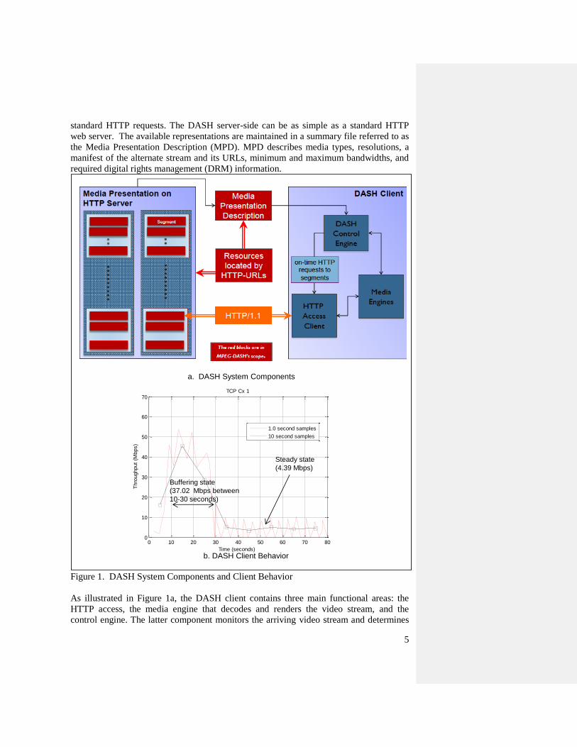
DASH Protocol Figure 1a illustrates the main components of a DASH-based video distribution system.
Multimedia content is encoded to one or more representations (different bit rates),
allowing the client (i.e., the media player) to request any part of a representation in units
of variable size blocks of data. The data content is made available to client devices by
5
standard HTTP requests. The DASH server-side can be as simple as a standard HTTP
web server. The available representations are maintained in a summary file referred to as
the Media Presentation Description (MPD). MPD describes media types, resolutions, a
manifest of the alternate stream and its URLs, minimum and maximum bandwidths, and
required digital rights management (DRM) information.
Figure 1. DASH System Components and Client Behavior
As illustrated in Figure 1a, the DASH client contains three main functional areas: the
HTTP access, the media engine that decodes and renders the video stream, and the
control engine. The latter component monitors the arriving video stream and determines
0 10 20 30 40 50 60 70 800
10
20
30
40
50
60
70
Time (seconds)
Thro
ughput
(Mbps)
TCP Cx 1
1.0 second samples
10 second samples
Buffering state
(37.02 Mbps between
10-30 seconds)
Steady state
(4.39 Mbps)
b. DASH Client Behavior
a. DASH System Components
6
when a lower or higher quality stream should be requested. The client will maintain a
playback buffer that serves to smooth variable content arrival rates to support the video
playback. The client requests a new segment (tagged with the desired bitrate) once the
playback buffer drops below a certain threshold. When the playback buffer is almost
empty, the client is likely to go into a ‘buffering’ state where it requests segments at a
high rate. The session therefore operates in one of two states: buffering or steady state.
While in a buffering state, the client requests data at a rate up to the available bandwidth
over the path between the server and the client. If conditions permit, the session will
attempt to find a ‘steady state’ where it requests segments at a rate necessary to playback
the content at a given encoded bitrate. In the analysis we present in this paper, we define
steady state as a time interval of at least 50 seconds where the session exhibits a stable
mean (i.e., observed mean over at least two 50 second intervals is within a tolerance of
10% variation). This assessment of ‘steady state’ is a network-oriented measure and is
potentially different from an assessment of ‘steady state’ at the application level. In future
work we will explore the interaction between network conditions, playback buffer
management, video encoder/decoder behaviors and the subsequent effects on perceived
quality.
Figure 1b illustrates the observed behavior of a Netflix client operating on a Windows
Desktop PC located at Clemson University. The results illustrate the first 80 seconds of a
Netflix streaming session over a high speed network (i.e., the available bandwidth
significantly exceeds the requirements of a Netflix session). The two curves plot the
evolution of the observed throughput of a single TCP connection that transfers video
content from the Netflix system to the client. The solid curve formed by the square data
points is based on 10 second throughput sampling intervals and the lighter dashed curve
is based on 1 second samples. The figure shows the initial buffering state and, once the
playback buffer is full, that the session moves into a steady state within about 35 seconds.
While this basic ‘waveform’ associated with DASH is similar across different client
devices that we have studied, we will show in our results that the detailed behavior of
each client device varies.
Methodology The research reported in this paper involves a measurement component and a simulation
component. We describe the methodology of each activity separately.
Measurement methodology
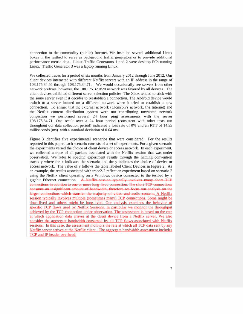
Figure 2 illustrates the measurement testbed that was used to monitor live Netflix
sessions. We created a private network that connected four different client devices: an
Xbox, a Roku device, a Windows desktop, and an Android Smartphone. The devices
were connected to the campus network either through a private gigabit Ethernet or
through an 802.11n network that was in turn directly connected to the campus network
through our private gigabit Ethernet. A high-definition monitor (capable of 1080p format)
was connected to the Xbox and Roku’s HDMI port. We monitored Netflix traffic by
obtaining network traces using tcpdump at the Linux Router. The router connects the
measurement testbed with Clemson University’s Network which provides a 10 Gbps
7
connection to the commodity (public) Internet. We installed several additional Linux
boxes in the testbed to serve as background traffic generators or to provide additional
performance metric data. Linux Traffic Generators 1 and 2 were desktop PCs running
Linux. Traffic Generator 3 was a laptop running Linux.
We collected traces for a period of six months from January 2012 through June 2012. Our
client devices interacted with different Netflix servers with an IP address in the range of
108.175.34.66 through 108.175.34.71. We would occasionally see servers from other
network prefixes, however, the 108.175.32.0/20 network was favored by all devices. The
client devices exhibited different server selection policies. The Xbox tended to stick with
the same server even if it decides to reestablish a connection. The Android device would
switch to a server located on a different network when it tried to establish a new
connection. To ensure that the external network (Clemson’s network, the Internet) and
the Netflix content distribution system were not contributing unwanted network
congestion we performed several 24 hour ping assessments with the server
108.175.34.71. One result over a 24 hour period (consistent with other tests run
throughout our data collection period) indicated a loss rate of 0% and an RTT of 14.55
milliseconds (ms) with a standard deviation of 0.64 ms.
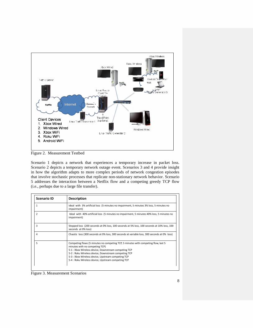
Figure 3 identifies five experimental scenarios that were considered. For the results
reported in this paper, each scenario consists of a set of experiments. For a given scenario
the experiments varied the choice of client device or access network. In each experiment,
we collected a trace of all packets associated with the Netflix session that was under
observation. We refer to specific experiment results through the naming convention
tracex-y where the x indicates the scenario and the y indicates the choice of device or
access network. The value of y follows the table labeled Client Devices in Figure 2. As
an example, the results associated with trace2-2 reflect an experiment based on scenario 2
using the Netflix client operating on a Windows device connected to the testbed by a
gigabit Ethernet connection. A Netflix session typically involves many short TCP
connections in addition to one or more long-lived connection. The short TCP connections
consume an insignificant amount of bandwidth, therefore we focus our analysis on the
larger connections which transfer the majority of video and audio content. A Netflix
session typically involves multiple (sometimes many) TCP connections. Some might be
short-lived and others might be long-lived. Our analysis examines the behavior of
specific TCP flows used by Netflix Sessions. In particular we monitor the throughput
achieved by the TCP connection under observation. The assessment is based on the rate
at which application data arrives at the client device from a Netflix server. We also
consider the aggregate bandwidth consumed by all TCP flows associated with Netflix
sessions. In this case, the assessment monitors the rate at which all TCP data sent by any
Netflix server arrives at the Netflix client. The aggregate bandwidth assessment includes
TCP and IP header overhead.
8
Figure 2. Measurement Testbed
Scenario 1 depicts a network that experiences a temporary increase in packet loss.
Scenario 2 depicts a temporary network outage event. Scenarios 3 and 4 provide insight
in how the algorithm adapts to more complex periods of network congestion episodes
that involve stochastic processes that replicate non-stationary network behavior. Scenario
5 addresses the interaction between a Netflix flow and a competing greedy TCP flow
(i.e., perhaps due to a large file transfer).
Figure 3. Measurement Scenarios
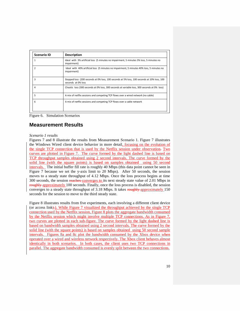
Scenario ID Description
1 Ideal with 3% artificial loss (5 minutes no impairment, 5 minutes 3% loss, 5 minutes no impairment)
2 Ideal with 40% artificial loss (5 minutes no impairment, 5 minutes 40% loss, 5 minutes no impairment)
3 Stepped loss (200 seconds at 0% loss, 100 seconds at 5% loss, 100 seconds at 10% loss, 100 seconds at 0% loss)
4 Chaotic loss (300 seconds at 0% loss, 300 seconds at variable loss, 300 seconds at 0% loss)
5 Competing flows (5 minutes no competing TCP, 5 minutes with competing flow, last 5 minutes with no competing TCP)5-1 : Xbox Wireless device, Downstream competing TCP5-2 : Roku Wireless device, Downstream competing TCP5-3 : Xbox Wireless device, Upstream competing TCP5-4 : Roku Wireless device, Upstream competing TCP
9
Simulation methodology
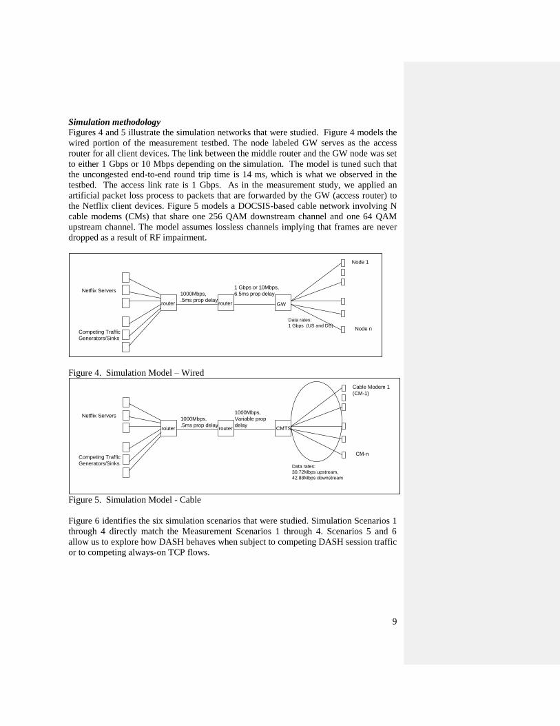
Figures 4 and 5 illustrate the simulation networks that were studied. Figure 4 models the
wired portion of the measurement testbed. The node labeled GW serves as the access
router for all client devices. The link between the middle router and the GW node was set
to either 1 Gbps or 10 Mbps depending on the simulation. The model is tuned such that
the uncongested end-to-end round trip time is 14 ms, which is what we observed in the
testbed. The access link rate is 1 Gbps. As in the measurement study, we applied an
artificial packet loss process to packets that are forwarded by the GW (access router) to
the Netflix client devices. Figure 5 models a DOCSIS-based cable network involving N
cable modems (CMs) that share one 256 QAM downstream channel and one 64 QAM
upstream channel. The model assumes lossless channels implying that frames are never
dropped as a result of RF impairment.
Figure 4. Simulation Model – Wired
Figure 5. Simulation Model - Cable
Figure 6 identifies the six simulation scenarios that were studied. Simulation Scenarios 1
through 4 directly match the Measurement Scenarios 1 through 4. Scenarios 5 and 6
allow us to explore how DASH behaves when subject to competing DASH session traffic
or to competing always-on TCP flows.
1000Mbps,
.5ms prop delay
Data rates:
1 Gbps (US and DS)
Node 1
Node n
GWrouter router
1 Gbps or 10Mbps,
6.5ms prop delayNetflix Servers
Competing Traffic
Generators/Sinks
1000Mbps,
.5ms prop delay
Data rates:
30.72Mbps upstream,
42.88Mbps downstream
Cable Modem 1
(CM-1)
CM-n
CMTSrouter router
1000Mbps,
Variable prop
delay
Netflix Servers
Competing Traffic
Generators/Sinks
10
Figure 6. Simulation Scenarios
Measurement Results
Scenario 1 results
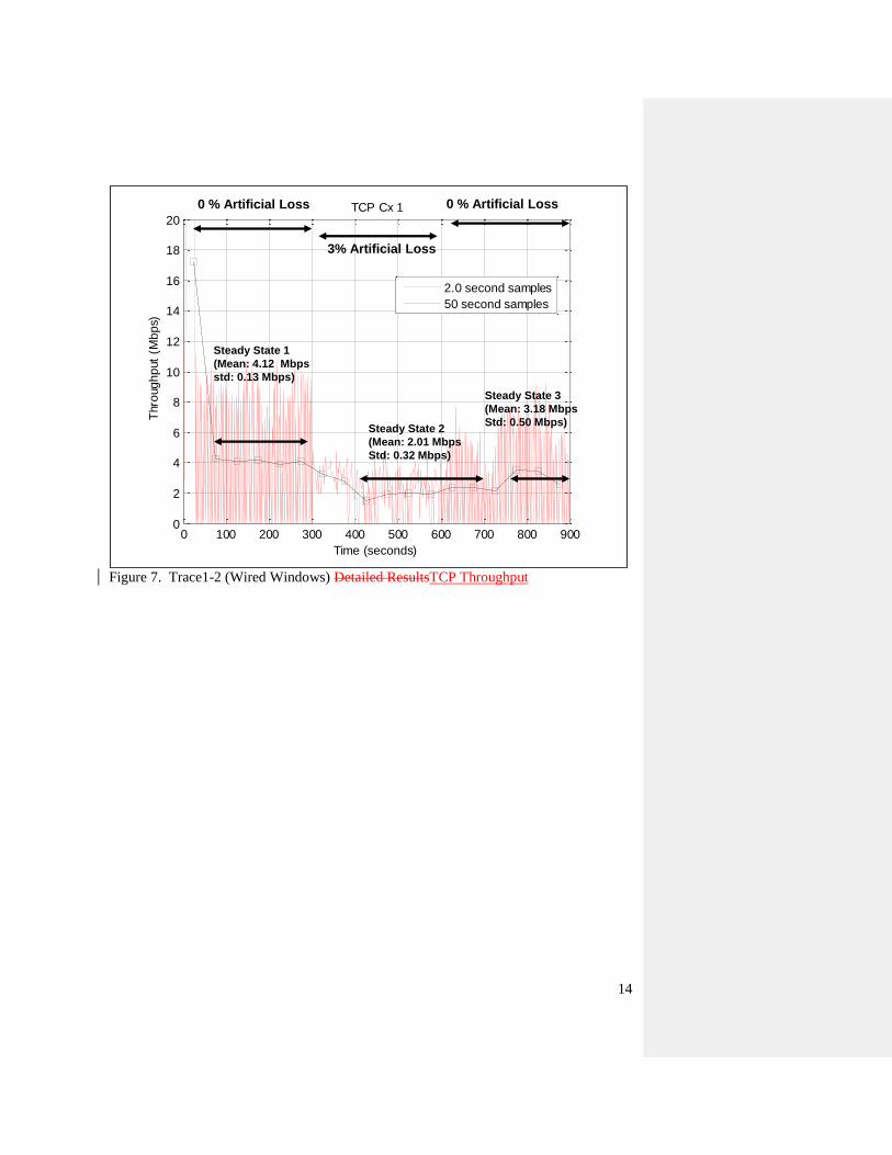
Figures 7 and 8 illustrate the results from Measurement Scenario 1. Figure 7 illustrates
the Windows Wired client device behavior in more detail, focusing on the evolution of
the single TCP connection that is used by the Netflix session under observation. Two
curves are plotted in Figure 7. The curve formed by the light dashed line is based on
TCP throughput samples obtained using 2 second intervals. The curve formed by the
solid line (with the square points) is based on samples obtained using 50 second
intervals. The initial buffer fill rate is roughly 40 Mbps (this data point cannot be seen in
Figure 7 because we set the y-axis limit to 20 Mbps). After 50 seconds, the session
moves to a steady state throughput of 4.12 Mbps. Once the loss process begins at time
300 seconds, the session reaches converges to its next steady state value of 2.01 Mbps in
roughly approximately 100 seconds. Finally, once the loss process is disabled, the session
converges to a steady state throughput of 3.18 Mbps. It takes roughly approximately 150
seconds for the session to move to the third steady state.
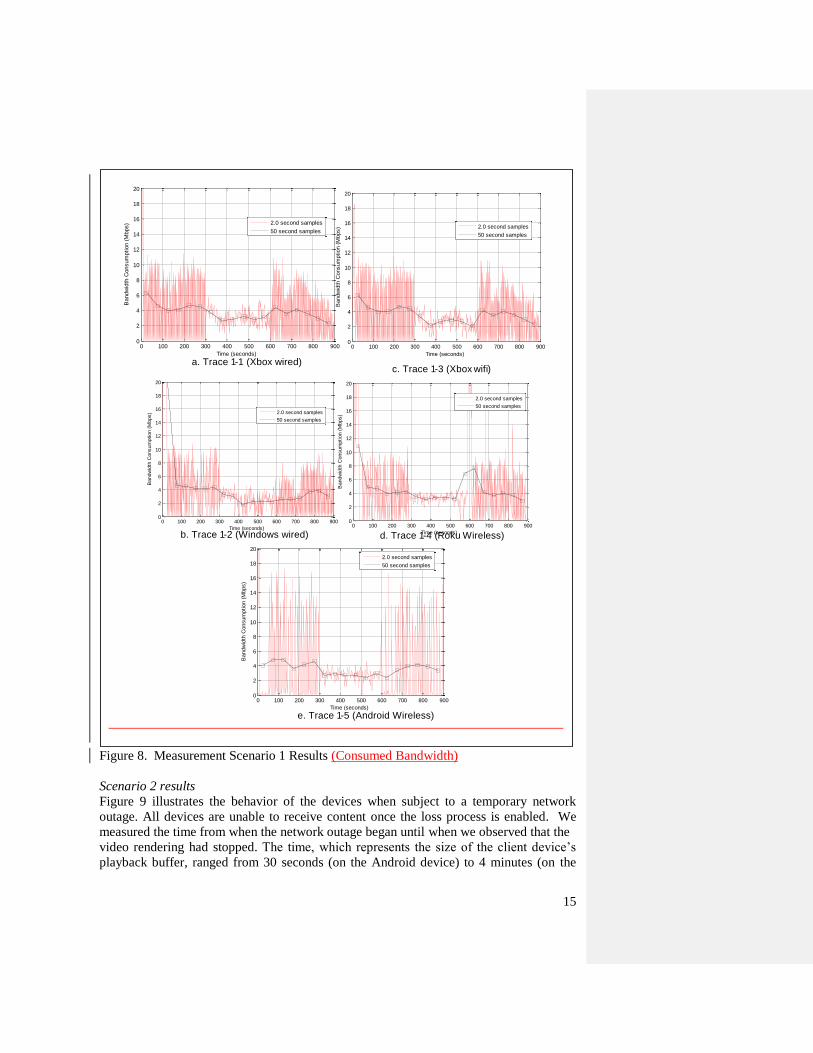
Figure 8 illustrates results from five experiments, each involving a different client device
(or access link).). While Figure 7 visualized the throughput achieved by the single TCP
connection used by the Netflix session, Figure 8 plots the aggregate bandwidth consumed
by the Netflix session which might involve multiple TCP connections. As in Figure 7,
two curves are plotted in each sub-figure. The curve formed by the light dashed line is
based on bandwidth samples obtained using 2 second intervals. The curve formed by the
solid line (with the square points) is based on samples obtained using 50 second sample
intervals. Figures 8a and 8c plot the bandwidth consumed by the Xbox device when
operated over a wired and wireless network respectively. The Xbox client behaves almost
identically in both scenarios. In both cases, the client uses two TCP connections in
parallel. The aggregate bandwidth consumed is evenly split between the two connections.
Scenario ID Description
1 Ideal with 3% artificial loss (5 minutes no impairment, 5 minutes 3% loss, 5 minutes no impairment)
2 Ideal with 40% artificial loss (5 minutes no impairment, 5 minutes 40% loss, 5 minutes no impairment)
3 Stepped loss (200 seconds at 0% loss, 100 seconds at 5% loss, 100 seconds at 10% loss, 100 seconds at 0% loss
4 Chaotic loss (300 seconds at 0% loss, 300 seconds at variable loss, 300 seconds at 0% loss)
5 A mix of netflix sessions and competing TCP flows over a wired network (no cable)
6 A mix of netflix sessions and competing TCP flows over a cable network
11
Figure 8 identifies the mean bandwidth consumption during three time periods that
represent the steady state periods that are observed. We refer to these intervals as
follows: (steady state) SS1: the intervals from 50-300 seconds; SS2: the interval from
400 to 550 seconds; SS3: the interval from 750 to 900 seconds. The wired Xbox Netflix
client consumes approximately 4.36 Mbps, 2.97 Mbps, and 2.93 Mbps in each of the
three intervals. The wireless device consumes roughly the same bandwidth.
The Windows wired results, illustrated in Figure 8b, is essentially the same as Figure 7
(i.e., the vast majority of audio/video data is transferred over the single long-lived TCP
connection). The bandwidth consumption observed in each steady state interval is
approximately 5% greater than the throughput observed in the intervals illustrated in
Figure 7. This is because the bandwidth consumption assessment includes TCP and IP
header overhead as well as additional TCP packets from a small number of ‘tiny’ (i.e.,
sent or received a very small amount of data) TCP connections that were active during
the experiment. Figure 8d illustrates the Roku device converges to steady state
throughputs of 4.37 Mbps, 3.31 Mbps and 3.55 Mbps. Further analysis (not presented in
this paper) indicates that in the time period 550 to 600 seconds, there were actually a
sequence of 5 short-lived TCP connections that were started. Each persisted for roughly
20 seconds. Once the loss process was stopped, a single connection was established that
transferred all subsequent content. Finally, Figure 8e visualizes the behavior of the
Netflix client on the Android device. Once loss started at time 300 seconds, multiple TCP
connections were observed. As with the Roku, the connections were started sequentially
and lasted about 20 seconds. The aggregate bandwidth consumed during this time period
was 2.61 Mbps. There are one, two or three figures that visualize the results from each
experiment. For example, Figures 8a and 8c each plot two graphs which together
visualize the throughput achieved by two parallel TCP connections that are used by the
Netflix client session running on an Xbox device connected by a wired or wireless
network respectively. Figure 8b plots the throughput achieved by the single TCP
connection used by a Windows Netflix client session. Two curves are plotted in each
graph. The light dashed line is based on TCP throughput samples obtained using 2
second intervals and the solid line is based on samples obtained using 30 second sample
intervals. Figures 8d and 8e each plots sequential TCP flows used by a Netflix client
running on a Roku and an Android device respectively. In all of our traces, the maximum
steady state throughput consumed by any session was 4.31 Mbps (observed with an Xbox
client session in Measurement Scenario 3-2). Table 1 provides the mean and standard
deviation of the observed throughput in each steady state period. For example, the first
row of Table 1 summarizes the results associated with Trace 1.1 which is the scenario1
experiment using the Xbox Wired device. The second column identifies the time period
during the trace that is being summarized. The third time identifies the setting of the
artificial loss process (i.e., it was either disabled or set to provide a random loss with an
packet loss rate of 3.0% during the time interval 300 to 600 seconds. The last three
columns provides information about the steady state throughput statistic (which is
considered during the time period given in column 2). The sample is based on 50 second
throughput samples. The fourth column identifies how many samples are considered. The
fifth and sixth columns provide the mean and standard variation of the steady state
12
throughput. For the Xbox experiments, the mean and standard deviation values in the
table are based on the samples from the two concurrent connections.
There clearly are differences across client devices were significant. It is difficult to
determine if observed differences in client behaviors is due to Netflix implementation
details or to the device TCP/IP stack. Based on the results from Measurement Scenario
1, we identify the following differences across client devices:
Netflix clients operating on Roku, Windows Desktops, and Android Smartphone
devices used a single TCP connection at a time. Only the Xbox client used two
TCP connections concurrently. All devices consumed steady state bandwidth in
the range of 4.35 to 4.40 Mbps during the first steady state interval. Based on
observation of the quality of the rendered video, we believe this reflects the
highest video quality level provided by Netflix.
(but the aggregate TCP throughput was always less than 4.3 Mbps).
The range of steady state throughputs bandwidth consumption achieved under
various controlled network scenarios varied significantly. Our results suggest that
Netflix application-level adaptation is conservative and that during periods of
network congestion appears to disengage.
The range of steady state throughputs bandwidth consumption achieved when loss
was active varied from 2.01 to 3.3120 Mbps. It is difficult to determine if
observed differences were due to Netflix implementation details or to the device
TCP/IP stack
Interestingly the Xbox converged to a throughput of 2.51 Mbps when connected
via gigabit Ethernet but only to 2.15 Mbps over WiFi. The Android device was
not able to maintain a TCP connection during this time period.
The range of times it takes the session to converge to new steady state
throughputs depends on the timescale that is used to define steady state. We
observed that Netflix reacts to congestion quickly (the example in Figure 7 shows
100 ms) but reacts more slowly to sudden increase in available bandwidth. Again
looking at Figure 7, it takes over 150 seconds for Netflix to increase the
application throughput change in throughput.
The range of steady state bandwidth consumption once the loss process is
disabled throughputs the sessions reach once the loss process is disabled ranges
from 2.973 Mbps to 3.7986 Mbps. This is less than the initial steady state
suggesting that Netflix reacts slowly to sudden increases in available bandwidth
after a period of sustained congestion. None of the devices restored the steady
state to the level observed before the emulated network congestion occurred.

13
14
Figure 7. Trace1-2 (Wired Windows) Detailed ResultsTCP Throughput
0 100 200 300 400 500 600 700 800 9000
2
4
6
8
10
12
14
16
18
20
Time (seconds)
Thro
ug
hp
ut
(Mb
ps)
TCP Cx 1
2.0 second samples
50 second samples
Steady State 1
(Mean: 4.12 Mbps
std: 0.13 Mbps)
Steady State 2
(Mean: 2.01 Mbps
Std: 0.32 Mbps)
Steady State 3
(Mean: 3.18 Mbps
Std: 0.50 Mbps)
0 % Artificial Loss 0 % Artificial Loss
3% Artificial Loss
15
Figure 8. Measurement Scenario 1 Results (Consumed Bandwidth)
Scenario 2 results
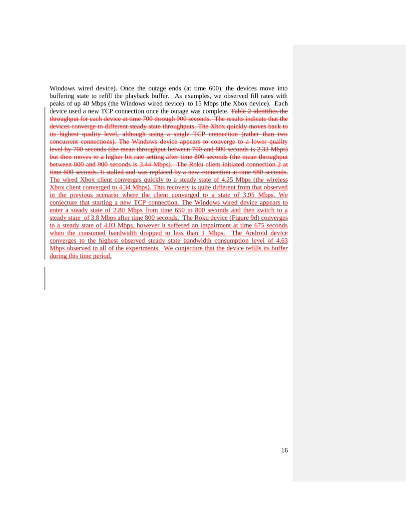
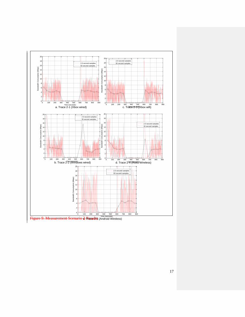
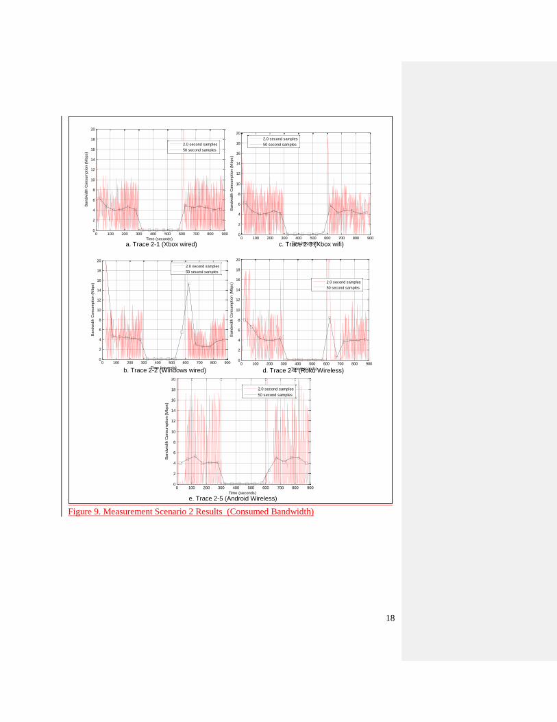
Figure 9 illustrates the behavior of the devices when subject to a temporary network
outage. All devices are unable to receive content once the loss process is enabled. We
measured the time from when the network outage began until when we observed that the
video rendering had stopped. The time, which represents the size of the client device’s
playback buffer, ranged from 30 seconds (on the Android device) to 4 minutes (on the
b. Trace 1-2 (Windows wired) d. Trace 1-4 (Roku Wireless)
e. Trace 1-5 (Android Wireless)
0 100 200 300 400 500 600 700 800 9000
2
4
6
8
10
12
14
16
18
20
Time (seconds)
Bandw
idth
Consum
ption (
Mbps)
2.0 second samples
50 second samples
a. Trace 1-1 (Xbox wired)c. Trace 1-3 (Xbox wifi)
0 100 200 300 400 500 600 700 800 9000
2
4
6
8
10
12
14
16
18
20
Time (seconds)
Bandw
idth
Consum
ption (
Mbps)
2.0 second samples
50 second samples
0 100 200 300 400 500 600 700 800 9000
2
4
6
8
10
12
14
16
18
20
Time (seconds)
Bandw
idth
Consum
ption (
Mbps)
2.0 second samples
50 second samples
0 100 200 300 400 500 600 700 800 9000
2
4
6
8
10
12
14
16
18
20
Time (seconds)
Bandw
idth
Consum
ption (
Mbps)
2.0 second samples
50 second samples
0 100 200 300 400 500 600 700 800 9000
2
4
6
8
10
12
14
16
18
20
Time (seconds)
Bandw
idth
Consum
ption (
Mbps)
2.0 second samples
50 second samples
16
Windows wired device). Once the outage ends (at time 600), the devices move into
buffering state to refill the playback buffer. As examples, we observed fill rates with
peaks of up 40 Mbps (the Windows wired device) to 15 Mbps (the Xbox device). Each
device used a new TCP connection once the outage was complete. Table 2 identifies the
throughput for each device at time 700 through 900 seconds. The results indicate that the
devices converge to different steady state throughputs. The Xbox quickly moves back to
its highest quality level, although using a single TCP connection (rather than two
concurrent connections). The Windows device appears to converge to a lower quality
level by 700 seconds (the mean throughput between 700 and 800 seconds is 2.33 Mbps)
but then moves to a higher bit rate setting after time 800 seconds (the mean throughput
between 800 and 900 seconds is 3.44 Mbps). The Roku client initiated connection 2 at
time 600 seconds. It stalled and was replaced by a new connection at time 680 seconds.
The wired Xbox client converges quickly to a steady state of 4.25 Mbps (the wireless
Xbox client converged to 4.34 Mbps). This recovery is quite different from that observed
in the previous scenario where the client converged to a state of 3.95 Mbps. We
conjecture that starting a new TCP connection. The Windows wired device appears to
enter a steady state of 2.80 Mbps from time 650 to 800 seconds and then switch to a
steady state of 3.8 Mbps after time 800 seconds. The Roku device (Figure 9d) converges
to a steady state of 4.03 Mbps, however it suffered an impairment at time 675 seconds
when the consumed bandwidth dropped to less than 1 Mbps. The Android device
converges to the highest observed steady state bandwidth consumption level of 4.63
Mbps observed in all of the experiments. We conjecture that the device refills its buffer
during this time period.
17
Figure 9. Measurement Scenario 2 Results
a. Trace 2-1 (Xbox wired) c. Trace 2-3 (Xbox wifi)
b. Trace 2-2 (Windows wired) d. Trace 2-4 (Roku Wireless)
e. Trace 2-5 (Android Wireless)
0 100 200 300 400 500 600 700 800 9000
2
4
6
8
10
12
14
16
18
20
Time (seconds)
Bandw
idth
Consum
ption (
Mbps)
2.0 second samples
50 second samples
0 100 200 300 400 500 600 700 800 9000
2
4
6
8
10
12
14
16
18
20
Time (seconds)
Bandw
idth
Consum
ption (
Mbps)
2.0 second samples
50 second samples
0 100 200 300 400 500 600 700 800 9000
2
4
6
8
10
12
14
16
18
20
Time (seconds)
Bandw
idth
Consum
ption (
Mbps)
2.0 second samples
50 second samples
0 100 200 300 400 500 600 700 800 9000
2
4
6
8
10
12
14
16
18
20
Time (seconds)
Bandw
idth
Consum
ption (
Mbps)
2.0 second samples
50 second samples
0 100 200 300 400 500 600 700 800 9000
2
4
6
8
10
12
14
16
18
20
Time (seconds)
Bandw
idth
Consum
ption (
Mbps)
2.0 second samples
50 second samples
18
Figure 9. Measurement Scenario 2 Results (Consumed Bandwidth)
a. Trace 2-1 (Xbox wired) c. Trace 2-3 (Xbox wifi)
b. Trace 2-2 (Windows wired) d. Trace 2-4 (Roku Wireless)
e. Trace 2-5 (Android Wireless)
0 100 200 300 400 500 600 700 800 9000
2
4
6
8
10
12
14
16
18
20
Time (seconds)
Bandw
idth
Consum
ption (
Mbps)
2.0 second samples
50 second samples
0 100 200 300 400 500 600 700 800 9000
2
4
6
8
10
12
14
16
18
20
Time (seconds)
Bandw
idth
Consum
ption (
Mbps)
2.0 second samples
50 second samples
0 100 200 300 400 500 600 700 800 9000
2
4
6
8
10
12
14
16
18
20
Time (seconds)
Bandw
idth
Consum
ption (
Mbps)
2.0 second samples
50 second samples
0 100 200 300 400 500 600 700 800 9000
2
4
6
8
10
12
14
16
18
20
Time (seconds)
Bandw
idth
Consum
ption (
Mbps)
2.0 second samples
50 second samples
0 100 200 300 400 500 600 700 800 9000
2
4
6
8
10
12
14
16
18
20
Time (seconds)
Bandw
idth
Consum
ption (
Mbps)
2.0 second samples
50 second samples
19
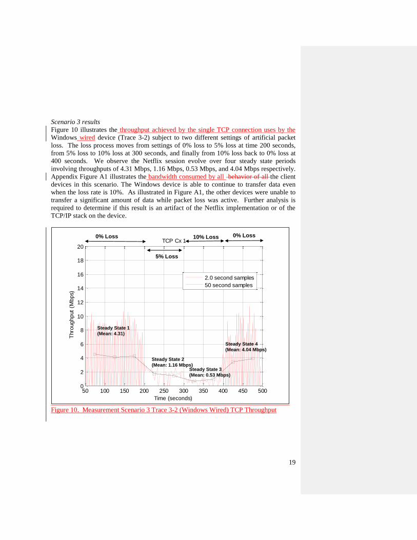
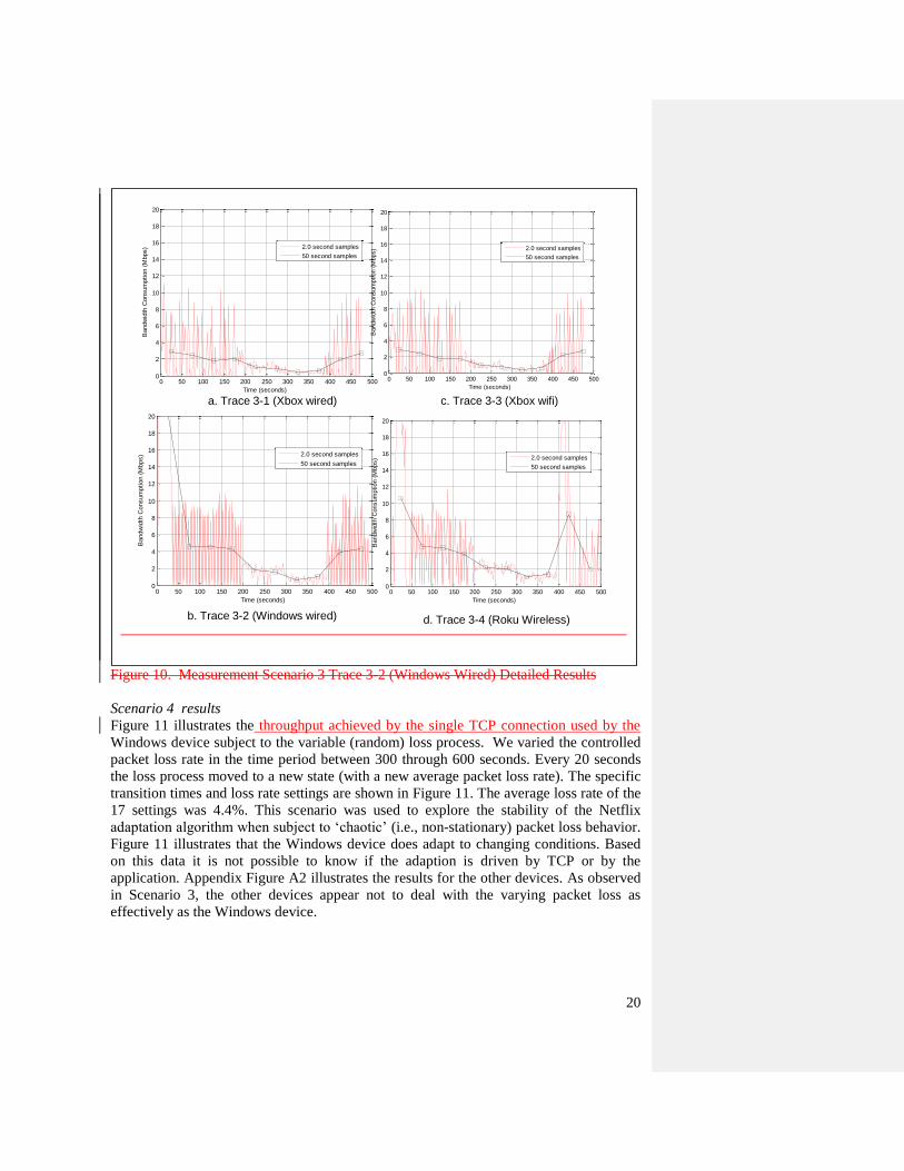
Scenario 3 results
Figure 10 illustrates the throughput achieved by the single TCP connection uses by the
Windows wired device (Trace 3-2) subject to two different settings of artificial packet
loss. The loss process moves from settings of 0% loss to 5% loss at time 200 seconds,
from 5% loss to 10% loss at 300 seconds, and finally from 10% loss back to 0% loss at
400 seconds. We observe the Netflix session evolve over four steady state periods
involving throughputs of 4.31 Mbps, 1.16 Mbps, 0.53 Mbps, and 4.04 Mbps respectively.
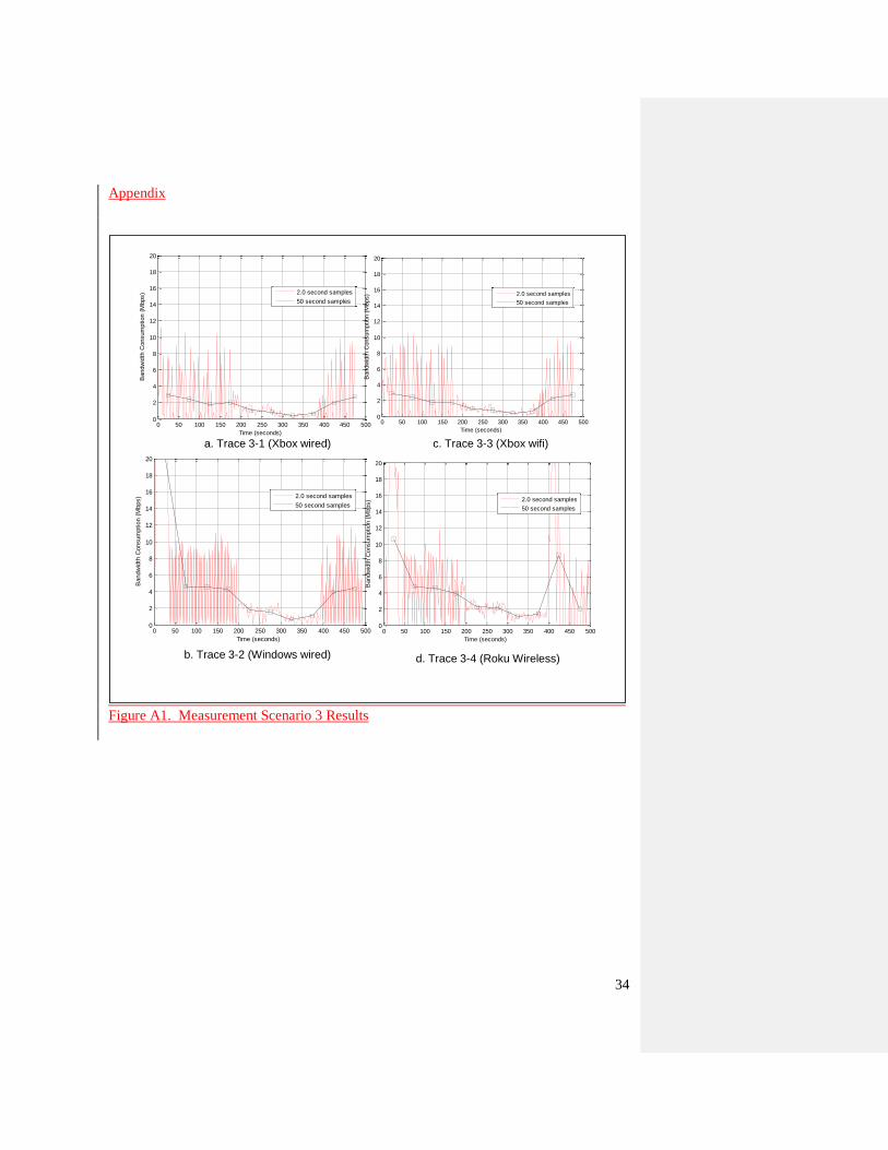
Appendix Figure A1 illustrates the bandwidth consumed by all behavior of all the client
devices in this scenario. The Windows device is able to continue to transfer data even
when the loss rate is 10%. As illustrated in Figure A1, the other devices were unable to
transfer a significant amount of data while packet loss was active. Further analysis is
required to determine if this result is an artifact of the Netflix implementation or of the
TCP/IP stack on the device.
Figure 10. Measurement Scenario 3 Trace 3-2 (Windows Wired) TCP Throughput
50 100 150 200 250 300 350 400 450 5000
2
4
6
8
10
12
14
16
18
20
Time (seconds)
Thro
ug
hp
ut
(Mb
ps)
TCP Cx 1
2.0 second samples
50 second samples
Steady State 1
(Mean: 4.31)
Steady State 2
(Mean: 1.16 Mbps)Steady State 3
(Mean: 0.53 Mbps)
Steady State 4
(Mean: 4.04 Mbps)
0% Loss
5% Loss
10% Loss 0% Loss
20
Figure 10. Measurement Scenario 3 Trace 3-2 (Windows Wired) Detailed Results
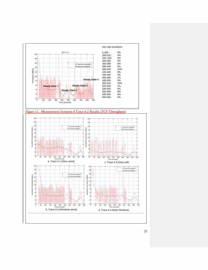
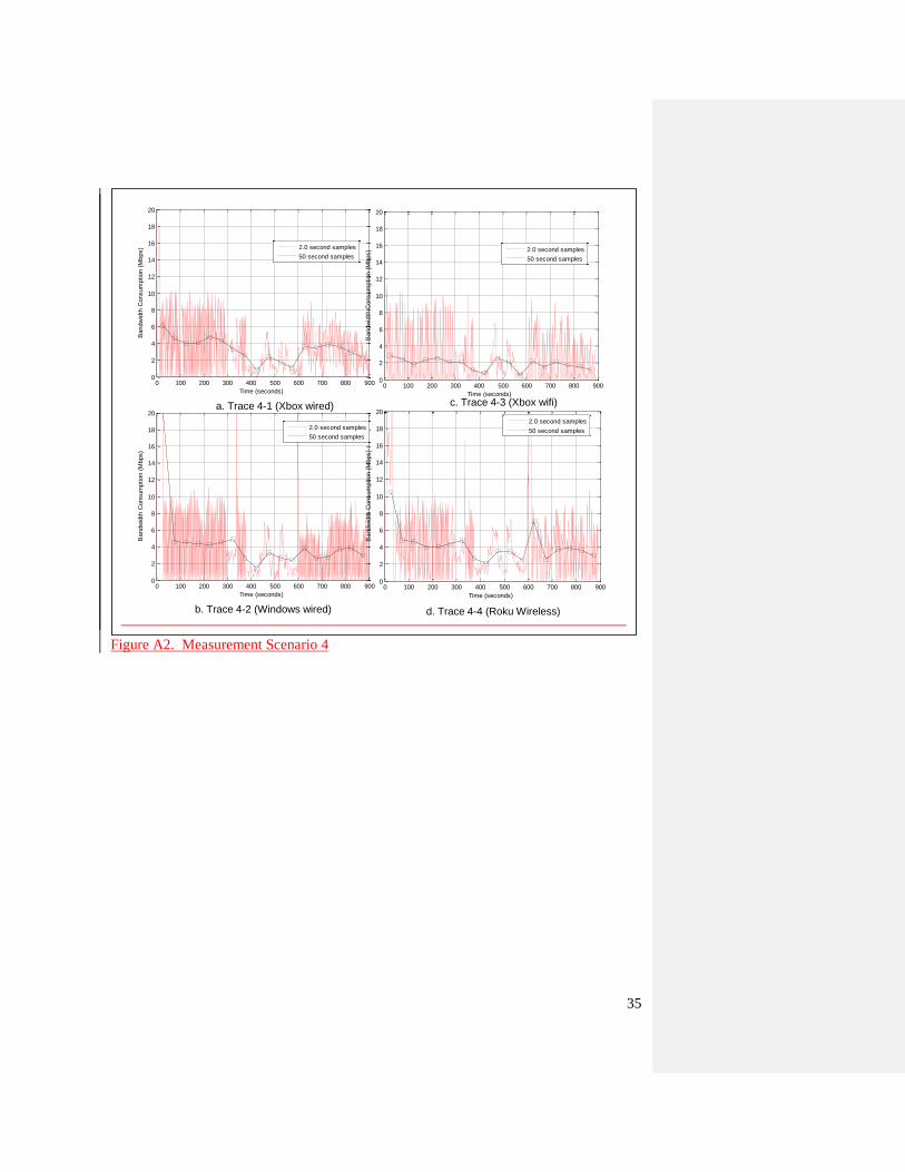
Scenario 4 results
Figure 11 illustrates the throughput achieved by the single TCP connection used by the
Windows device subject to the variable (random) loss process. We varied the controlled
packet loss rate in the time period between 300 through 600 seconds. Every 20 seconds
the loss process moved to a new state (with a new average packet loss rate). The specific
transition times and loss rate settings are shown in Figure 11. The average loss rate of the
17 settings was 4.4%. This scenario was used to explore the stability of the Netflix
adaptation algorithm when subject to ‘chaotic’ (i.e., non-stationary) packet loss behavior.
Figure 11 illustrates that the Windows device does adapt to changing conditions. Based
on this data it is not possible to know if the adaption is driven by TCP or by the
application. Appendix Figure A2 illustrates the results for the other devices. As observed
in Scenario 3, the other devices appear not to deal with the varying packet loss as
effectively as the Windows device.
a. Trace 3-1 (Xbox wired) c. Trace 3-3 (Xbox wifi)
b. Trace 3-2 (Windows wired) d. Trace 3-4 (Roku Wireless)
0 50 100 150 200 250 300 350 400 450 5000
2
4
6
8
10
12
14
16
18
20
Time (seconds)
Bandw
idth
Consum
ption (
Mbps)
2.0 second samples
50 second samples
0 50 100 150 200 250 300 350 400 450 5000
2
4
6
8
10
12
14
16
18
20
Time (seconds)
Bandw
idth
Consum
ption (
Mbps)
2.0 second samples
50 second samples
0 50 100 150 200 250 300 350 400 450 5000
2
4
6
8
10
12
14
16
18
20
Time (seconds)
Bandw
idth
Consum
ption (
Mbps)
2.0 second samples
50 second samples
0 50 100 150 200 250 300 350 400 450 5000
2
4
6
8
10
12
14
16
18
20
Time (seconds)
Bandw
idth
Consum
ption (
Mbps)
2.0 second samples
50 second samples
21
Figure 11. Measurement Scenario 4 Trace 4-2 Results (TCP Throughput)
0 100 200 300 400 500 600 700 800 9000
2
4
6
8
10
12
14
16
18
20
Time (seconds)
Thro
ug
hp
ut
(Mb
ps)
TCP Cx 1
2.0 second samples
50 second samples
loss rate transitions
0-300 : 0%
300-320 : 4%
320- 340 3%
340-360 0%
360-380 0%
380-400 8%
400-420 10%
420-440 9%
440-460 3%
460-480 1%
480-500 5%
500-520 10%
520-540 1%
540-560 4%
560-580 8%
580-600 9%
600-900 0%
Steady State 1
Steady State 2
Steady State 3
Steady State 4
a. Trace 4-1 (Xbox wired) c. Trace 4-3 (Xbox wifi)
b. Trace 4-2 (Windows wired) d. Trace 4-4 (Roku Wireless)
0 50 100 150 200 250 300 350 400 450 5000
2
4
6
8
10
12
14
16
18
20
Time (seconds)
Bandw
idth
Consum
ption (
Mbps)
2.0 second samples
50 second samples
0 50 100 150 200 250 300 350 400 450 5000
2
4
6
8
10
12
14
16
18
20
Time (seconds)
Bandw
idth
Consum
ption (
Mbps)
2.0 second samples
50 second samples
0 50 100 150 200 250 300 350 400 450 5000
2
4
6
8
10
12
14
16
18
20
Time (seconds)
Bandw
idth
Consum
ption (
Mbps)
2.0 second samples
50 second samples
0 50 100 150 200 250 300 350 400 450 5000
2
4
6
8
10
12
14
16
18
20
Time (seconds)
Bandw
idth
Consum
ption (
Mbps)
2.0 second samples
50 second samples
22
Figure 11. Measurement Scenario 4 Trace 4-2 Results
Scenario 5 results
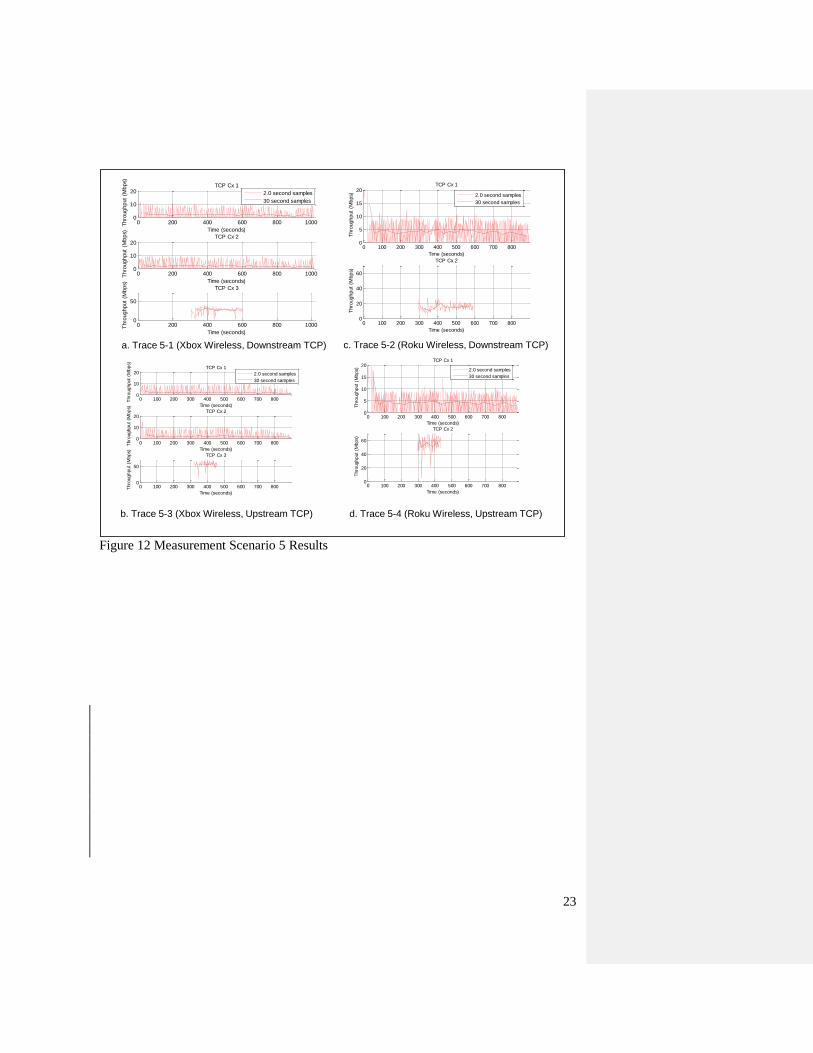
Figure 12 illustrates the results from Scenario 5. We defined four experiments, identified
as Trace 5-1 through Trace 5-4. Trace 5-1 involved the Xbox wireless device and Trace
5-2 involved the Roku wireless device. These traces demonstrate the effect of the
competing TCP flow downstream while Trace 5-3 and 5-4 involved an upstream TCP
flow. In all four experiments, a Netflix session is established at time 0 seconds. At time
300 seconds, the competing TCP flow is initiated between Traffic Generators 1 and 3.
We used iperf to generate competing TCP traffic. To generate competing downstream
traffic, iperf generates application traffic at the Traffic Generator located on Clemson’s
network destined for iperf set to sink arriving data at the Traffic Generator located on the
wireless network. Upstream traffic is generated simply by reversing the
sending/receiving roles of the Traffic Generators. The wireless AP was a Linksys
EA3500 configured to support 802.11n using 20 or 40 MHz channels in the 2.4 GHz ISM
band and in the 5.0 GHz band. Due to the campus WiFi network, our ‘rogue’ AP was
subject to significant interference. We observed significant variation in the competing
TCP flow’s throughput. We conjecture that interference was causing the AP to switch
back and forth between 20 MHz and 40 MHz channels frequently. In the best conditions
we observed a maximum sustained upstream TCP throughput of 63 Mbps. In the
downstream case, the results were more unpredictable. In some cases, we observed
throughput up to 63 Mbps. Most of the time however, we observe throughput in the 15-
25 Mbps range.
Figure 12a illustrates the results from Experiment 5-1. The graphs labeled TCP Cx1 and
TCP Cx2 visualize the two concurrent TCP connections used by the Xbox Netflix client.
The graph labeled TCP Cx3 visualizes the throughput achieved by the competing TCP
flow. Figure 12a identifies the three steady state periods the Xbox client experiences.
Table’s 3 and 4 shows the average throughput (and standard deviation) of the steady state
1 and steady state 2 periods of each trace for the scenarios that involve a downstream and
then an upstream competing TCP. The results suggest that the Netflix session is impacted
more by a competing flow that is oriented downstream rather than upstream. For the
Xbox, prior to when the competing flow begins (at time 300 seconds), the aggregate TCP
throughput achieved by the Netflix session is 4.19 Mbps. Once the competing flow
begins, the aggregate Xbox TCP throughput drops by 11.9% to 3.70 Mbps. Once the loss
process terminates however, the Xbox TCP throughput converges to an even lower rate
of 3.06 Mbps. This is consistent with the Roku device which evolves from 3.93Mbps to
3.72 Mbps and finally to 3.21 Mbps. We conclude that Netflix adapts quickly to drops in
available bandwidth but reacts very cautiously as available bandwidth is restored.
23
Figure 12 Measurement Scenario 5 Results
0 200 400 600 800 10000
10
20 TCP Cx 1
Time (seconds)
Thro
ug
hp
ut
(Mb
ps)
2.0 second samples
30 second samples
0 200 400 600 800 10000
10
20 TCP Cx 2
Time (seconds)
Thro
ug
hp
ut
(Mb
ps)
0 200 400 600 800 10000
50
TCP Cx 3
Time (seconds)
Thro
ug
hp
ut
(Mb
ps)
a. Trace 5-1 (Xbox Wireless, Downstream TCP) c. Trace 5-2 (Roku Wireless, Downstream TCP)
b. Trace 5-3 (Xbox Wireless, Upstream TCP) d. Trace 5-4 (Roku Wireless, Upstream TCP)
0 100 200 300 400 500 600 700 8000
5
10
15
20 TCP Cx 1
Time (seconds)
Thro
ug
hp
ut
(Mb
ps)
2.0 second samples
30 second samples
0 100 200 300 400 500 600 700 8000
20
40
60
TCP Cx 2
Time (seconds)
Thro
ug
hp
ut
(Mb
ps)
0 100 200 300 400 500 600 700 8000
10
20 TCP Cx 1
Time (seconds)
Thro
ug
hp
ut
(Mb
ps)
2.0 second samples
30 second samples
0 100 200 300 400 500 600 700 8000
10
20 TCP Cx 2
Time (seconds)
Thro
ug
hp
ut
(Mb
ps)
0 100 200 300 400 500 600 700 8000
50
TCP Cx 3
Time (seconds)
Thro
ug
hp
ut
(Mb
ps)
0 100 200 300 400 500 600 700 8000
5
10
15
20 TCP Cx 1
Time (seconds)
Thro
ug
hp
ut
(Mb
ps)
2.0 second samples
30 second samples
0 100 200 300 400 500 600 700 8000
20
40
60
TCP Cx 2
Time (seconds)
Thro
ug
hp
ut
(Mb
ps)
24
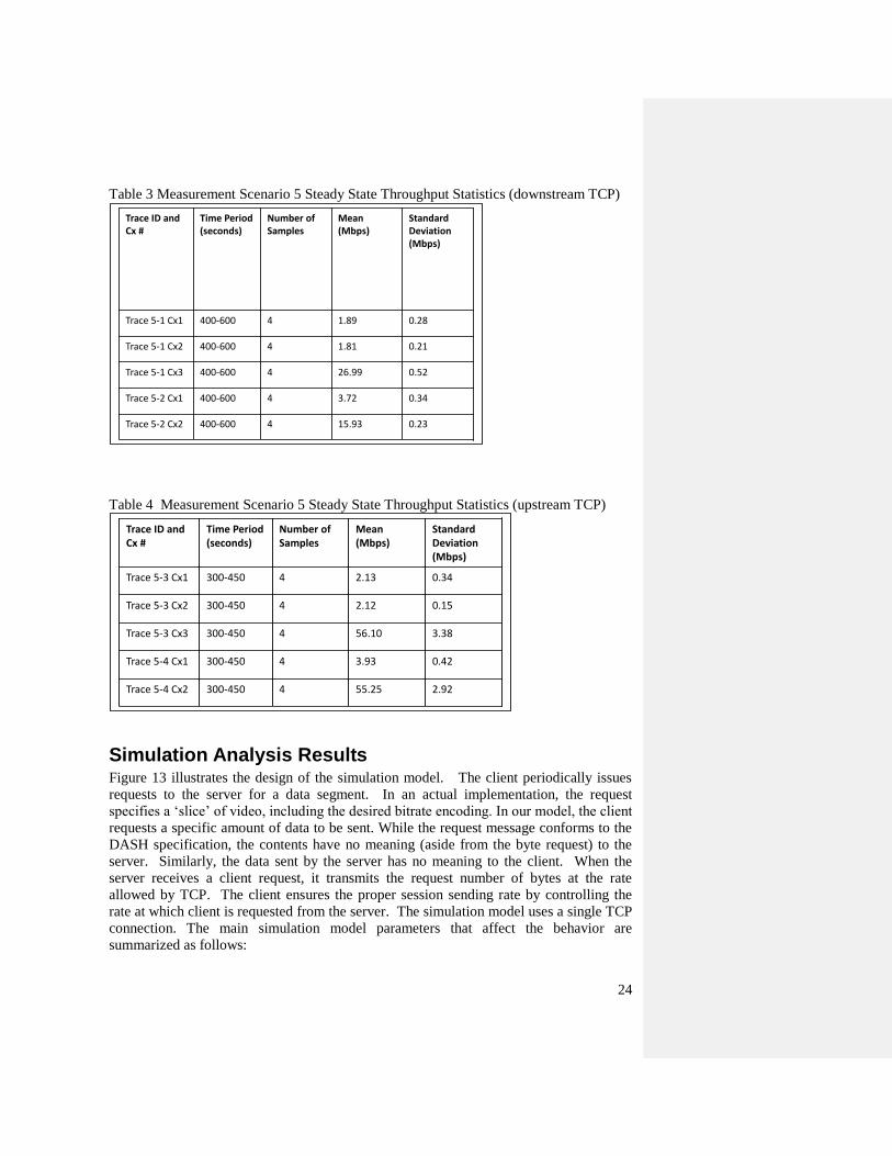
Table 3 Measurement Scenario 5 Steady State Throughput Statistics (downstream TCP)
Table 4 Measurement Scenario 5 Steady State Throughput Statistics (upstream TCP)
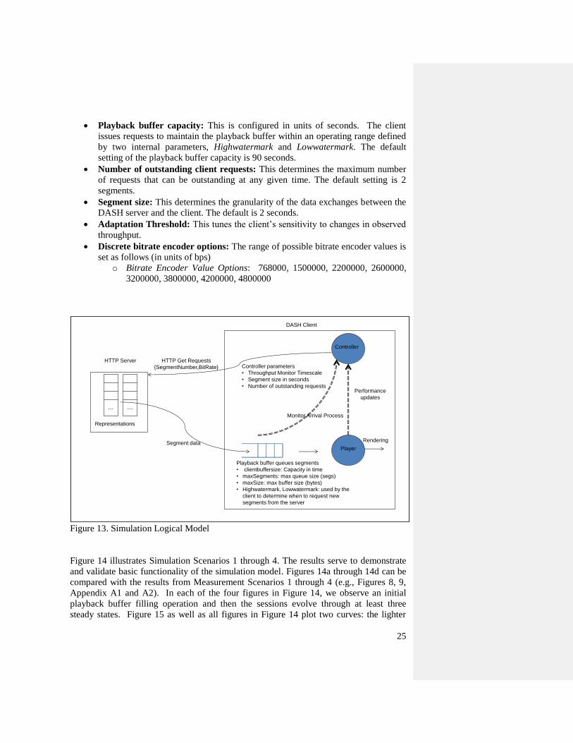
Simulation Analysis Results Figure 13 illustrates the design of the simulation model. The client periodically issues
requests to the server for a data segment. In an actual implementation, the request
specifies a ‘slice’ of video, including the desired bitrate encoding. In our model, the client
requests a specific amount of data to be sent. While the request message conforms to the
DASH specification, the contents have no meaning (aside from the byte request) to the
server. Similarly, the data sent by the server has no meaning to the client. When the
server receives a client request, it transmits the request number of bytes at the rate
allowed by TCP. The client ensures the proper session sending rate by controlling the
rate at which client is requested from the server. The simulation model uses a single TCP
connection. The main simulation model parameters that affect the behavior are
summarized as follows:
Trace ID and Cx #
Time Period (seconds)
Number of Samples
Mean (Mbps)
Standard Deviation (Mbps)
Trace 5-1 Cx1 400-600 4 1.89 0.28
Trace 5-1 Cx2 400-600 4 1.81 0.21
Trace 5-1 Cx3 400-600 4 26.99 0.52
Trace 5-2 Cx1 400-600 4 3.72 0.34
Trace 5-2 Cx2 400-600 4 15.93 0.23
Trace ID and Cx #
Time Period (seconds)
Number of Samples
Mean (Mbps)
Standard Deviation (Mbps)
Trace 5-3 Cx1 300-450 4 2.13 0.34
Trace 5-3 Cx2 300-450 4 2.12 0.15
Trace 5-3 Cx3 300-450 4 56.10 3.38
Trace 5-4 Cx1 300-450 4 3.93 0.42
Trace 5-4 Cx2 300-450 4 55.25 2.92
25
Playback buffer capacity: This is configured in units of seconds. The client
issues requests to maintain the playback buffer within an operating range defined
by two internal parameters, Highwatermark and Lowwatermark. The default
setting of the playback buffer capacity is 90 seconds.
Number of outstanding client requests: This determines the maximum number
of requests that can be outstanding at any given time. The default setting is 2
segments.
Segment size: This determines the granularity of the data exchanges between the
DASH server and the client. The default is 2 seconds.
Adaptation Threshold: This tunes the client’s sensitivity to changes in observed
throughput.
Discrete bitrate encoder options: The range of possible bitrate encoder values is
set as follows (in units of bps)
o Bitrate Encoder Value Options: 768000, 1500000, 2200000, 2600000,
3200000, 3800000, 4200000, 4800000
Figure 13. Simulation Logical Model
Figure 14 illustrates Simulation Scenarios 1 through 4. The results serve to demonstrate
and validate basic functionality of the simulation model. Figures 14a through 14d can be
compared with the results from Measurement Scenarios 1 through 4 (e.g., Figures 8, 9,
Appendix A1 and A2). In each of the four figures in Figure 14, we observe an initial
playback buffer filling operation and then the sessions evolve through at least three
steady states. Figure 15 as well as all figures in Figure 14 plot two curves: the lighter
25
HTTP Server
DASH Client
Playback buffer queues segments
• clientbuffersize: Capacity in time
• maxSegments: max queue size (segs)
• maxSize: max buffer size (bytes)
• Highwatermark, Lowwatermark: used by the
client to determine when to request new
segments from the server
Representations
Player
Controller
HTTP Get Requests
{SegmentNumber,BitRate}
Segment data
Controller parameters
• Throughput Monitor Timescale
• Segment size in seconds
• Number of outstanding requests
Monitor Arrival Process
Rendering
Performance
updates
… …
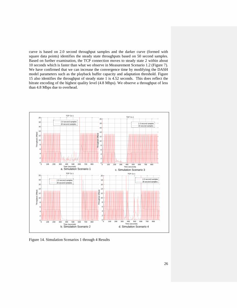
26
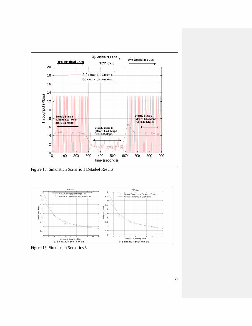
curve is based on 2.0 second throughput samples and the darker curve (formed with
square data points) identifies the steady state throughputs based on 50 second samples.
Based on further examination, the TCP connection moves to steady state 2 within about
10 seconds which is faster than what we observe in Measurement Scenario 1.2 (Figure 7).
We have confirmed that we can increase the convergence time by modifying the DASH
model parameters such as the playback buffer capacity and adaptation threshold. Figure
15 also identifies the throughput of steady state 1 is 4.52 seconds. This does reflect the
bitrate encoding of the highest quality level (4.8 Mbps). We observe a throughput of less
than 4.8 Mbps due to overhead.
Figure 14. Simulation Scenarios 1 through 4 Results
b. Simulation Scenario 2 d. Simulation Scenario 4
a. Simulation Scenario 1 c. Simulation Scenario 3
0 100 200 300 400 500 600 700 8000
2
4
6
8
10
12
14
16
18
20 TCP Cx 1
Time (seconds)
Thro
ug
hp
ut
(Mb
ps)
2.0 second samples
30 second samples
0 100 200 300 400 500 600 700 8000
2
4
6
8
10
12
14
16
18
20 TCP Cx 1
Time (seconds)
Thro
ug
hp
ut
(Mb
ps)
2.0 second samples
30 second samples
0 100 200 300 400 500 600 700 8000
2
4
6
8
10
12
14
16
18
20 TCP Cx 1
Time (seconds)
Thro
ug
hp
ut
(Mb
ps)
2.0 second samples
30 second samples
0 100 200 300 400 500 600 700 8000
2
4
6
8
10
12
14
16
18
20 TCP Cx 1
Time (seconds)
Thro
ug
hp
ut
(Mb
ps)
2.0 second samples
30 second samples
27
Figure 15. Simulation Scenario 1 Detailed Results
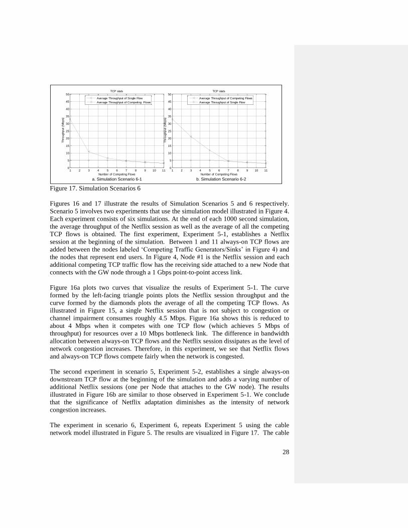
Figure 16. Simulation Scenarios 5
0 100 200 300 400 500 600 700 800 9000
2
4
6
8
10
12
14
16
18
20
Time (seconds)
Thro
ug
hp
ut
(Mb
ps)
TCP Cx 1
2.0 second samples
50 second samples
Steady State 1
(Mean: 4.52 Mbps
std: 0.13 Mbps)
Steady State 2
(Mean: 1.43 Mbps
Std: 0.15Mbps)
Steady State 3
(Mean: 4.44 Mbps
Std: 0.12 Mbps)
0 % Artificial Loss0 % Artificial Loss
3% Artificial Loss
a. Simulation Scenario 5-1 b. Simulation Scenario 5-2
1 2 3 4 5 6 7 8 9 10 110
0.5
1
1.5
2
2.5
3
3.5
4
4.5
5
Number of Competing Flows
Thro
ug
hp
ut
(Mb
ps)
TCP stats
Average Throughput of Single Flow
Average Throughput of Competing Flows
1 2 3 4 5 6 7 8 9 10 110
0.5
1
1.5
2
2.5
3
3.5
4
4.5
5
Number of Competing Flows
Thro
ug
hp
ut
(Mb
ps)
TCP stats
Average Throughput of Competing Flows
Average Throughput of Single Flow
28
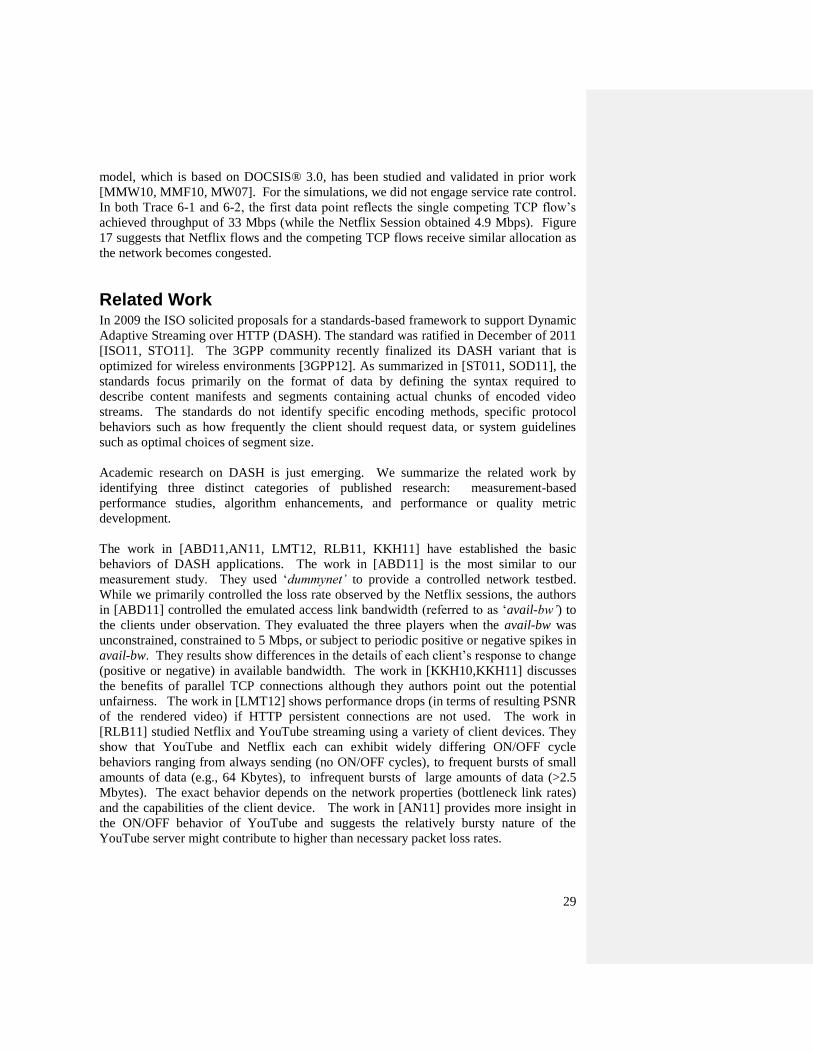
Figure 17. Simulation Scenarios 6
Figures 16 and 17 illustrate the results of Simulation Scenarios 5 and 6 respectively.
Scenario 5 involves two experiments that use the simulation model illustrated in Figure 4.
Each experiment consists of six simulations. At the end of each 1000 second simulation,
the average throughput of the Netflix session as well as the average of all the competing
TCP flows is obtained. The first experiment, Experiment 5-1, establishes a Netflix
session at the beginning of the simulation. Between 1 and 11 always-on TCP flows are
added between the nodes labeled ‘Competing Traffic Generators/Sinks’ in Figure 4) and
the nodes that represent end users. In Figure 4, Node #1 is the Netflix session and each
additional competing TCP traffic flow has the receiving side attached to a new Node that
connects with the GW node through a 1 Gbps point-to-point access link.
Figure 16a plots two curves that visualize the results of Experiment 5-1. The curve
formed by the left-facing triangle points plots the Netflix session throughput and the
curve formed by the diamonds plots the average of all the competing TCP flows. As
illustrated in Figure 15, a single Netflix session that is not subject to congestion or
channel impairment consumes roughly 4.5 Mbps. Figure 16a shows this is reduced to
about 4 Mbps when it competes with one TCP flow (which achieves 5 Mbps of
throughput) for resources over a 10 Mbps bottleneck link. The difference in bandwidth
allocation between always-on TCP flows and the Netflix session dissipates as the level of
network congestion increases. Therefore, in this experiment, we see that Netflix flows
and always-on TCP flows compete fairly when the network is congested.
The second experiment in scenario 5, Experiment 5-2, establishes a single always-on
downstream TCP flow at the beginning of the simulation and adds a varying number of
additional Netflix sessions (one per Node that attaches to the GW node). The results
illustrated in Figure 16b are similar to those observed in Experiment 5-1. We conclude
that the significance of Netflix adaptation diminishes as the intensity of network
congestion increases.
The experiment in scenario 6, Experiment 6, repeats Experiment 5 using the cable
network model illustrated in Figure 5. The results are visualized in Figure 17. The cable
a. Simulation Scenario 6-1 b. Simulation Scenario 6-2
1 2 3 4 5 6 7 8 9 10 110
5
10
15
20
25
30
35
40
45
50
Number of Competing Flows
Thro
ug
hp
ut
(Mb
ps)
TCP stats
Average Throughput of Single Flow
Average Throughput of Competing Flows
1 2 3 4 5 6 7 8 9 10 110
5
10
15
20
25
30
35
40
45
50
Number of Competing Flows
Thro
ug
hp
ut
(Mb
ps)
TCP stats
Average Throughput of Competing Flows
Average Throughput of Single Flow
29
model, which is based on DOCSIS® 3.0, has been studied and validated in prior work
[MMW10, MMF10, MW07]. For the simulations, we did not engage service rate control.
In both Trace 6-1 and 6-2, the first data point reflects the single competing TCP flow’s
achieved throughput of 33 Mbps (while the Netflix Session obtained 4.9 Mbps). Figure
17 suggests that Netflix flows and the competing TCP flows receive similar allocation as
the network becomes congested.
Related Work In 2009 the ISO solicited proposals for a standards-based framework to support Dynamic
Adaptive Streaming over HTTP (DASH). The standard was ratified in December of 2011
[ISO11, STO11]. The 3GPP community recently finalized its DASH variant that is
optimized for wireless environments [3GPP12]. As summarized in [ST011, SOD11], the
standards focus primarily on the format of data by defining the syntax required to
describe content manifests and segments containing actual chunks of encoded video
streams. The standards do not identify specific encoding methods, specific protocol
behaviors such as how frequently the client should request data, or system guidelines
such as optimal choices of segment size.
Academic research on DASH is just emerging. We summarize the related work by
identifying three distinct categories of published research: measurement-based
performance studies, algorithm enhancements, and performance or quality metric
development.
The work in [ABD11,AN11, LMT12, RLB11, KKH11] have established the basic
behaviors of DASH applications. The work in [ABD11] is the most similar to our
measurement study. They used ‘dummynet’ to provide a controlled network testbed.
While we primarily controlled the loss rate observed by the Netflix sessions, the authors
in [ABD11] controlled the emulated access link bandwidth (referred to as ‘avail-bw’) to
the clients under observation. They evaluated the three players when the avail-bw was
unconstrained, constrained to 5 Mbps, or subject to periodic positive or negative spikes in
avail-bw. They results show differences in the details of each client’s response to change
(positive or negative) in available bandwidth. The work in [KKH10,KKH11] discusses
the benefits of parallel TCP connections although they authors point out the potential
unfairness. The work in [LMT12] shows performance drops (in terms of resulting PSNR
of the rendered video) if HTTP persistent connections are not used. The work in
[RLB11] studied Netflix and YouTube streaming using a variety of client devices. They
show that YouTube and Netflix each can exhibit widely differing ON/OFF cycle
behaviors ranging from always sending (no ON/OFF cycles), to frequent bursts of small
amounts of data (e.g., 64 Kbytes), to infrequent bursts of large amounts of data (>2.5
Mbytes). The exact behavior depends on the network properties (bottleneck link rates)
and the capabilities of the client device. The work in [AN11] provides more insight in
the ON/OFF behavior of YouTube and suggests the relatively bursty nature of the
YouTube server might contribute to higher than necessary packet loss rates.
30
The work in [ACH12, CMP11, EKG11, LBG11, SSH11] consider possible
improvements to DASH-based streaming. [ACH12] considers the benefits of using
Scalable Video Coding (SVC) outweigh the additional overhead. The authors identify
optimal approaches for determining which block should be selected next. The block
might be data that will improve the video quality of a frame whose base layer has already
arrived or it might be a block corresponding to the base layer of a frame further out in
time). The work in [SSH11] shows that DASH applications extended to support SVC can
improve cache hit rates in typical CDN distribution networks. The work in [CMP11,
LBG11, EKG11] focus on the adaptation algorithm. All approaches seek to react to
persistent impairment by dropping to lower bitrate content and then restore to higher
quality content as conditions improve. The challenge is to do this so as perceived quality
is maximized.
All of the related work involves assessing performance in some manner. As summarized
in [OS12], the standards have defined various metrics including throughput,
request/response time, buffer levels, adaptation event counts. The work in [DAJ11]
provides a more comprehensive framework by identifying metrics such as join time (the
time from when the session is initiated by the user until when video rendering begins),
percentage of time the viewing is halted due to buffering (i.e., when the video rendering
stops and the user is shown a message indicating “Buffering in Progress”), and the rate
of buffering events. Finally, the work in [NEE11A, NEE11B, XST09] describes the
subtle flicker effects that are especially evident in low compute power devices such as
smartphones.
Conclusions Video streaming has been widely deployed and studied for decades. However DASH-
based streaming has not been widely studied simply because it is a new protocol. Our
main research objective is to understand the impact of adaptive applications on
bandwidth control mechanisms within a broadband access network.
In our measurement results, we have observed a wide range of behaviors across different
client devices and network behaviors. The highlights of our results include the following:
The range of steady state throughputs achieved under controlled packet loss
settings varied significantly.
The range of times it takes the session to converge to new steady state
throughputs also varied. One challenge that we experienced was determining
when the session achieved steady state. Based on our results, we find that the
Netflix implementations that we studied appeared to behave conservatively and
tended to react over timescales in the 50 to 100 second range.
The range of throughputs the sessions reach once the loss process is disabled
varied by device. This aspect of the protocol represents a challenging design
issue: if the client attempts to use increased levels of available bandwidth quickly
it runs the risk of having to reduce bandwidth in the near future if congestion is
intermittent. On the other hand, the client should not give up available bandwidth
unnecessarily.
31
The playback buffer sizes ranged from 30 seconds (on the Android device) to 4
minutes (on the Windows wired device). The average size of the client request
ranged from 1.8 Mbytes to 3.57 Mbytes (we did not show these results in the
paper).
The measurement experiments that involved wireless provides further insight in
the behavior of Netflix. However additional analysis is required to better
characterize and assess Netflix in realistic wireless networks.
Our simulation results help us better understand the measurement results. For example,
by changing the simulation model’s playback buffer capacity and adaption threshold
values we can observe behaviors that move the model closer or further from the
behaviors we observed in the measurement analysis. The results from simulation
scenarios 5 and 6 suggest that the significance of application adaptation diminishes as the
intensity of network congestion increases. Based on this insight, we conjecture that the
observed throughput variability during the period 300 to 700 seconds of Measurement
scenario 4 (Trace 4-2 illustrated in Figure 11) is driven by TCP congestion control rather
than application adaptation. In future work we plan to explore in more detail the
parameter space associated with DASH applications. In particular we want to explore
how certain parameter settings, such as playback buffer capacity and adaptation
responsiveness, impact system performance. We would also like to better understand the
behavior of large numbers of competing Netflix sessions. Specific questions are:
Does Netflix give up too much bandwidth when competing with greedy, always-
on TCP flows?
Can aggregate Netflix traffic be accurately modeled using tractable analytic
methods?
Can the optimal buffer capacity or the most appropriate AQM strategy be
identified for a given router or CMTS subject to an expected number of Netflix
sessions?
The obvious next step must address the issue of how network impairment (which leads to
subsequent changes to bandwidth consumption) impact the perceived quality. The
performance of video streaming is challenging to assess since the details of the video
encoding and decoding process significantly impact the perceived quality., especially
when the streams are subject to network impairment. In future work we will correlate
network measurable results with perceived quality.
References [3GPP12] 3GPP TS 26.247 version 10.1.0 Release 10: “Transparent End-to-end Packet
Switched Streaming Service (PSS); Progressive Download and Dynamic Adaptive
Service over HTTP”, 3GPP, January 2012, available online at
http://www.etsi.org/deliver/etsi_ts/126200_126299/126247/10.01.00_60/ts_126247v1001
00p.pdf
Formatted: Bulleted + Level: 1 + Aligned at: 0.29" + Indent at: 0.54"
32
[ABD11] S. Akhshabi, A. Begen, C. Dovrolis, “An Experimental Evaluation of Rate-
Adaptation Algorithms in Adaptive Streaming over HTTP”, Proceedings of ACM
MMSys, February 2011.
[ACH12] T. Andelin, V. Chetty, D. Harbaugh, S. Warnick, D. Zappala, “Quality
Selection for Dynamic Adaptive Streaming over HTTP with Scalable Video Coding”,
Proceedings of ACM MMSys, February 2012.
[AN11] S. Alcock, R. Nelson, “Application Flow Control in YouTube Video Streams”,
ACM SIGCOMM Computer Communication Review, April 2011.
[CMP11] L. Cicco, S. Mascolo, V. Palmisano, “Feedback Control for Adaptive Live
Video Streaming”, Proceedings of MMSys’11, February 2011.
[DAJ11] F. Dobrian, A. Awan, D. Joseph, A. Ganjamm J. Zhan, V. Sekar, I. Stoica, H.
Zhang, “Understanding the Impact of Video Quality on User Engagement”, Proceedings
of SIGCOMM’11, August 2011.
[EKG11] K. Evensen, D. Kaspar, C. Griwodz, P. Halvorsen, A. Hansen, P. Engelstad,
“Improving the Performance of Quality-Adaptive Video Streaming over Multiple
Heterogeneous Access Networks”, Proceedings of MMSys’11, February 2011.
[ISO11] ISO/IEC, “Information technology — MPEG systems technologies — Part 6:
Dynamic adaptive streaming over HTTP (DASH)”, Jan 2011, available online at
http://mpeg.chiariglione.org/working_documents/mpeg-dash/dash-dis.zip
[KKH10] R. Kuschnig, I. Kofler, H. Hellwagner, “Improving Internet Video Streaming
Performance by Parallel TCP-based Request-Response Streams”, Proceedings of IEEE
CCNC 2010, January 2010.
[KKH11] R. Kuschnig, I. Kofler, H. Hellwagner, “Evaluation of HTTP-based Request-
Response Streams for Internet Video Streaming”, Proceedings of MMSys’11, February
2011.
[LBG11] C. Liu, I. Bouazizi, M. Gabbouj, “Rate Adaptation for Adaptive HTTP
Streaming”, Proceedings of ACM MMSys, February 2011.
[LMT12] S. Lederer, C. Muller, C. Timmerer, “Dynamic Adaptive Streaming over HTTP
Dataset”, Proceedings of ACM MMSys, February 2012.
[MW07] J. Martin, J. Westall, “A Simulation Model of the DOCSIS Protocol”,
Simulation: Transactions of the Society for Modeling and Simulation International, 83(2),
139-155 (2007).
33
[MWF10] J. Martin, J. Westall, J. Finkelstein, G. Hart, T. Shaw, G. White, R.
Woundy, "Cable Modem Buffer Management in DOCSIS Networks", Proceedings of
the IEEE Sarnoff 2010 Symposium, (Princeton University, Princeton NJ, April 2010).
[MMW10] S. Moser, J. Martin, J. Westall, B. Dean, "The Role of Max-min Fairness in
DOCSIS 3.0 Downstream Channel Bonding", Proceedings of the IEEE Sarnoff 2010
Symposium, (Princeton University, Princeton NJ, April 2010).
[MT11] C. Muller, C. Timmerer, “A Testbed for the Dynamic Adaptive Streaming over
Http Featuring Session Mobility”, Proceedings of ACM MMSys, February 2011.
[NEE11A] P. Ni, R. Eg., A. Eichhorn, C. Griwodz, P. Halvorsen, “Flicker Effects in
Adaptive Video Streaming to Handheld Devices”, Proceedings of MM’11, November
2011.
[NEE11B] P. Ni, R. Eg., A. Eichhorn, C. Griwodz, P. Halvorsen, “Spatial Flicker Effect
in Video Scaling”, Proceedings of Quality of Multimedia Experience (QoMEX)
Workshop, September, 2011.
[OS12] O. Oyman, S. Singh, “Quality of Experience for HTTP Adaptive Streaming
Services”, IEEE Communications Magazine, April 2012.
[RLB11] A. Roa, Y. Lim, C. Barakat, A. Legout, D. Towsley, W. Dabbous, “Network
Characteristics of Video Streaming Traffic”, Proceedings of ACM CoNEXT Conference,
December 2011.
[SOD11] I. Sodagar, “The MPEG-DASH Standard for Multimedia Streaming Over the
Internet”, IEEE Multimedia magazine, October/December 2011.
[SOP12] S. Singh, O. Oyman, A. Papathanassiou, D. Chatterjee, J. Andrews, “Video
Capacity and QoE Enhancements in LTE”, submitted.
[SSH11] Y. Sanchez, T. Schierl, C. Hellge, T. Wiegand, D. Vleeshauwer, W. Keekwijck,
Y. Louedec, “iDash: Improved Dynamic Adaptive Streaming over HTTP using Scalable
Video Coding”, Proceedings of ACM MMSys, February 2011.
[STO11] T. Stockhammer, “Dynamic Adaptive Streaming over HTTP – Standards and
Design Principles”, Proceedings of the MMSys’11, February 2011.
[XST09] J. Xia, Y. Shi, K. Tuenissen, I. Heynderick, “Perceivable Artifacts in
Compressed Video and their Relation to Video Quality”, Elsevier Signal Processing:
Image Communication, vol 24, 2009
34
Appendix
Figure A1. Measurement Scenario 3 Results
a. Trace 3-1 (Xbox wired) c. Trace 3-3 (Xbox wifi)
b. Trace 3-2 (Windows wired) d. Trace 3-4 (Roku Wireless)
0 50 100 150 200 250 300 350 400 450 5000
2
4
6
8
10
12
14
16
18
20
Time (seconds)
Bandw
idth
Consum
ption (
Mbps)
2.0 second samples
50 second samples
0 50 100 150 200 250 300 350 400 450 5000
2
4
6
8
10
12
14
16
18
20
Time (seconds)
Bandw
idth
Consum
ption (
Mbps)
2.0 second samples
50 second samples
0 50 100 150 200 250 300 350 400 450 5000
2
4
6
8
10
12
14
16
18
20
Time (seconds)
Bandw
idth
Consum
ption (
Mbps)
2.0 second samples
50 second samples
0 50 100 150 200 250 300 350 400 450 5000
2
4
6
8
10
12
14
16
18
20
Time (seconds)
Bandw
idth
Consum
ption (
Mbps)
2.0 second samples
50 second samples
35
Figure A2. Measurement Scenario 4
a. Trace 4-1 (Xbox wired) c. Trace 4-3 (Xbox wifi)
b. Trace 4-2 (Windows wired) d. Trace 4-4 (Roku Wireless)
0 100 200 300 400 500 600 700 800 9000
2
4
6
8
10
12
14
16
18
20
Time (seconds)
Bandw
idth
Consum
ption (
Mbps)
2.0 second samples
50 second samples
0 100 200 300 400 500 600 700 800 9000
2
4
6
8
10
12
14
16
18
20
Time (seconds)
Bandw
idth
Consum
ption (
Mbps)
2.0 second samples
50 second samples
0 100 200 300 400 500 600 700 800 9000
2
4
6
8
10
12
14
16
18
20
Time (seconds)
Bandw
idth
Consum
ption (
Mbps)
2.0 second samples
50 second samples
0 100 200 300 400 500 600 700 800 9000
2
4
6
8
10
12
14
16
18
20
Time (seconds)
Bandw
idth
Consum
ption (
Mbps)
2.0 second samples
50 second samples
Recommended