Analytical Solutions and Conservation Laws ofModels Describing Heat Transfer Through
Extended Surfaces
Partner Luyanda Ndlovu
School of Computational and Applied Mathematics,University of the Witwatersrand,Johannesburg, South Africa.
A dissertation submitted to the Faculty of Science,University of the Witwatersrand, in fulfillment of therequirements for the degree of Master of Science.
March 28, 2013

Declaration
I declare that this project is my own, unaided work. It is being submitted
as partial fulfilment of the Degree of Master of Science at the University of
the Witwatersrand, Johannesburg. It has not been submitted before for any
degree or examination in any other University.
Partner Luyanda Ndlovu
March 28, 2013

Abstract
The search for solutions to the important differential equations arising in ex-
tended surface heat transfer continues unabated. Extended surfaces, in the
form of longitudinal fins are considered. First we consider the steady state
problem and then the transient heat transfer models. Here, thermal conduc-
tivity and heat transfer coefficient are assumed to be functions of temperature.
Thermal conductivity is considered to be given by the power law in one case
and by the linear function of temperature in the other; whereas heat transfer
coefficient is only given by the power law. Explicit analytical expressions for
the temperature profile, fin efficiency and heat flux for steady state problems
are derived using the one-dimensional Differential Transform Method (1D DT-
M). The obtained results from 1D DTM are compared with the exact solutions
to verify the accuracy of the proposed method. The results reveal that the 1D
DTM can achieve suitable results in predicting the solutions of these prob-
lems. The effects of some physical parameters such as the thermo-geometric
fin parameter and thermal conductivity gradient, on temperature distribution
are illustrated and explained. Also, we apply the two-dimensional Differential
Transform Method (2D DTM) to models describing transient heat transfer in
longitudinal fins. Furthermore, conservation laws for transient heat conduction
equations are derived using the direct method and the multiplier method, and
finally we find Lie point symmetries associated with the conserved vectors.

Acknowledgments
I would like to thank my supervisor Professor R.J. Moitsheki for his support
and kindness. Throughout the year, he has been an inspiring mentor who kept
faith through adversity and encouraged me to always try hard. Even during
the times when I was struggling and ready to give up, his perseverance and
support helped me greatly. I will never forget his invaluable words of advice
and our interesting and funny conversations. To my fellow friends Simphiwe,
Moshe and Rahab, thank you for your everlasting guidance at the DECMA
laboratory.
I must acknowledge the support I received from my wonderful family who
have always been there for me. Qinisani at Nedbank and Oskar I have to thank
you for your guidance, love and support. You were my pillars of strength and
everything that I have been able to accomplish is because you were right by
my side. To my brothers Siyabonga, Richard and my sister Patience, your
support has always meant so much to me, thank you for never letting me give
up on anything. A very special dedication and honour to my parents Dineo
Bakela and Nelson Ndlovu, may your souls rest in peace.
This research was supported by the National Research Foundation (NRF)
under GUID:82302.

Contents
1 Introduction 1
1.1 Literature review . . . . . . . . . . . . . . . . . . . . . . . . . . 1
1.2 Aims and objectives of the dissertation . . . . . . . . . . . . . . 4
1.3 Outline of the dissertation . . . . . . . . . . . . . . . . . . . . . 4
2 Formulae and theory 6
2.1 Introduction . . . . . . . . . . . . . . . . . . . . . . . . . . . . . 6
2.2 Differential Transform Methods . . . . . . . . . . . . . . . . . . 6
2.2.1 1D-Differential Transform Method . . . . . . . . . . . . . 6
2.2.2 2D-Differential Transform Method . . . . . . . . . . . . . 8
2.3 Lie point symmetries . . . . . . . . . . . . . . . . . . . . . . . . 10
2.4 Conservation laws . . . . . . . . . . . . . . . . . . . . . . . . . . 11
2.4.1 Direct method . . . . . . . . . . . . . . . . . . . . . . . . 12
2.4.2 Multiplier method . . . . . . . . . . . . . . . . . . . . . 13
2.5 Concluding remarks . . . . . . . . . . . . . . . . . . . . . . . . . 13
3 Mathematical models describing heat transfer in longitudinal
fins 14
3.1 Introduction . . . . . . . . . . . . . . . . . . . . . . . . . . . . . 14
3.2 Mathematical models . . . . . . . . . . . . . . . . . . . . . . . . 14
i

CONTENTS ii
3.3 Concluding remarks . . . . . . . . . . . . . . . . . . . . . . . . . 18
4 Analytical solutions for steady heat transfer in fins of various
profiles 19
4.1 Introduction . . . . . . . . . . . . . . . . . . . . . . . . . . . . . 19
4.2 Power law thermal conductivity . . . . . . . . . . . . . . . . . . 21
4.2.1 Comparison of exact and analytical (DTM) solutions
given m = n . . . . . . . . . . . . . . . . . . . . . . . . . 21
4.2.2 Distinct exponents, m = n . . . . . . . . . . . . . . . . . 26
4.3 Linear thermal conductivity . . . . . . . . . . . . . . . . . . . . 33
4.3.1 The rectangular profile, f(x) = 1 . . . . . . . . . . . . . 33
4.3.2 The convex parabolic profile, f(x) = x1/2 . . . . . . . . . 35
4.3.3 The exponential profile, f(x) = eσx . . . . . . . . . . . . 39
4.4 Fin efficiency and heat flux . . . . . . . . . . . . . . . . . . . . . 42
4.4.1 Fin efficiency . . . . . . . . . . . . . . . . . . . . . . . . 42
4.4.2 Heat flux . . . . . . . . . . . . . . . . . . . . . . . . . . 43
4.5 Discussion of results . . . . . . . . . . . . . . . . . . . . . . . . 43
4.6 Concluding remarks . . . . . . . . . . . . . . . . . . . . . . . . . 48
5 Application of the 2D DTM to transient heat transfer prob-
lems 49
5.1 Introduction . . . . . . . . . . . . . . . . . . . . . . . . . . . . . 49
5.2 Rectangular profile . . . . . . . . . . . . . . . . . . . . . . . . . 50
5.2.1 Solution for n = 1 . . . . . . . . . . . . . . . . . . . . . . 50
5.2.2 Solution for n = 0 . . . . . . . . . . . . . . . . . . . . . . 52
5.2.3 Solution for n = 2 . . . . . . . . . . . . . . . . . . . . . . 53
5.2.4 Solution for n = 3 . . . . . . . . . . . . . . . . . . . . . . 53
5.3 Convex parabolic profile . . . . . . . . . . . . . . . . . . . . . . 53

CONTENTS iii
5.3.1 Solution for n = 1 . . . . . . . . . . . . . . . . . . . . . . 54
5.3.2 Solution for n = 0 . . . . . . . . . . . . . . . . . . . . . . 55
5.3.3 Solution for n = 2 . . . . . . . . . . . . . . . . . . . . . . 55
5.4 Discussion of results . . . . . . . . . . . . . . . . . . . . . . . . 55
5.5 Concluding remarks . . . . . . . . . . . . . . . . . . . . . . . . . 62
6 Conservation laws and associated Lie point symmetries for
equations describing transient heat transfer in fins 63
6.1 Introduction . . . . . . . . . . . . . . . . . . . . . . . . . . . . . 63
6.2 Nonlinear equation with power law thermal conductivity . . . . 64
6.2.1 Direct method . . . . . . . . . . . . . . . . . . . . . . . . 64
6.2.2 Multiplier method . . . . . . . . . . . . . . . . . . . . . 68
6.3 Nonlinear equation with linear thermal conductivity . . . . . . . 71
6.3.1 Direct method . . . . . . . . . . . . . . . . . . . . . . . . 71
6.3.2 Multiplier method . . . . . . . . . . . . . . . . . . . . . 74
6.4 Conserved vectors and associated point symmetries . . . . . . . 76
6.4.1 Case m = n (m = −1, m = 0) . . . . . . . . . . . . . . . 77
6.4.2 Case m = n (n = −1, m = −1, m = 0) . . . . . . . . . . 79
6.5 Concluding remarks . . . . . . . . . . . . . . . . . . . . . . . . . 82
7 Conclusions 83
Bibliography 85

List of Figures
3.1 Schematic representation of a longitudinal fin . . . . . . . . . . 15
4.1 Comparison of analytical and exact solutions. Here we chose
n = 1, M = 0.7 . . . . . . . . . . . . . . . . . . . . . . . . . . . 25
4.2 Comparison of analytical and exact solutions. Here we chose
n = 2, M = 0.5 . . . . . . . . . . . . . . . . . . . . . . . . . . . 26
4.3 Temperature distribution in an exponential fin. The thermal
conductivity exponent is greater than the heat transfer coeffi-
cient exponent, (n,m) = (3, 2) . . . . . . . . . . . . . . . . . . . 28
4.4 Temperature distribution in an exponential fin, (n,m) = (2, 3) . 29
4.5 Temperature distribution in a rectangular fin. The thermal con-
ductivity exponent is less than the heat transfer coefficient ex-
ponent (n,m) = (2, 3) . . . . . . . . . . . . . . . . . . . . . . . . 30
4.6 Temperature distribution in a rectangular fin, (n,m) = (3, 2) . . 31
4.7 Temperature distribution in a convex fin. The thermal conduc-
tivity exponent is less than the heat transfer coefficient exponent
(n,m) = (2, 3) . . . . . . . . . . . . . . . . . . . . . . . . . . . . 32
4.8 Temperature distribution in a convex fin, (n,m) = (3, 2) . . . . 33
iv

LIST OF FIGURES v
4.9 Temperature profile in a longitudinal rectangular fin with linear
thermal conductivity and varying values of n. Here β = 0.5 and
M = 1.5 are fixed . . . . . . . . . . . . . . . . . . . . . . . . . . 36
4.10 Temperature profile in a longitudinal convex parabolic fin with
linear thermal conductivity and varying values of n. Here β =
0.5 and M = 1.5 are fixed . . . . . . . . . . . . . . . . . . . . . 38
4.11 Temperature profile in a longitudinal fin of exponential profile
with linear thermal conductivity and varying values of n. Here
β = 0.5 and M = 1.5 are fixed . . . . . . . . . . . . . . . . . . . 41
4.12 Fin efficiency of a longitudinal rectangular fin. Here β = 0.75. . 42
4.13 Base heat flux in a longitudinal rectangular fin with linear ther-
mal conductivity. Here β = 0.1. . . . . . . . . . . . . . . . . . . 44
4.14 Heat flux across a longitudinal rectangular fin with power law
thermal conductivity. Here n−m > 0, Bi = 0.01. . . . . . . . . 44
4.15 Heat flux across a longitudinal rectangular fin with power law
thermal conductivity. Here n−m < 0, Bi = 0.01. . . . . . . . . 45
4.16 Base heat flux in a longitudinal rectangular fin with power law
thermal conductivity. Here n−m = 0, Bi = 0.01. . . . . . . . . 45
5.1 Transient temperature distribution in a rectangular fin with lin-
ear thermal conductivity, n = 1, β = 1,M = 6 . . . . . . . . . . 56
5.2 Transient temperature distribution in a rectangular fin with lin-
ear thermal conductivity, n = 1, β = 1, τ = 1.2 . . . . . . . . . . 56
5.3 Transient temperature distribution in a rectangular fin with lin-
ear thermal conductivity, n = 1,M = 2.5, τ = 1.2 . . . . . . . . 57
5.4 Transient temperature distribution in a rectangular fin with lin-
ear thermal conductivity, n = 0, β = 1, τ = 1.2 . . . . . . . . . . 57

LIST OF FIGURES vi
5.5 Transient temperature distribution in a rectangular fin with lin-
ear thermal conductivity, M = 40, β = 1, τ = 1.2 . . . . . . . . . 58
5.6 Transient temperature distribution in a rectangular fin with lin-
ear thermal conductivity, M = β = n = 1, with varying x . . . . 58
5.7 Transient temperature distribution in a rectangular fin with lin-
ear thermal conductivity, M = β = n = 1 . . . . . . . . . . . . . 59
5.8 Transient temperature distribution in a rectangular fin with lin-
ear thermal conductivity, M = 0.75, β = 1, n = 1 . . . . . . . . . 59
5.9 Transient temperature distribution in a convex parabolic fin
with linear thermal conductivity, β = 1, τ = 0.2 . . . . . . . . . 60
5.10 Transient temperature distribution in a rectangular and con-
vex parabolic fin with linear thermal conductivity, M = 6, β =
1, τ = 1.2 . . . . . . . . . . . . . . . . . . . . . . . . . . . . . . 60

List of Tables
4.1 Results of the DTM and Exact Solutions for n = 1, M = 0.7 . . 24
4.2 Results of the DTM and Exact Solutions for n = 2, M = 0.5 . . 25
vii

Chapter 1
Introduction
1.1 Literature review
In the study of heat transfer, an extended surface (also known as a fin) is
a solid that extends from a hot body to increase the rate of heat transfer
to the surrounding fluid. A growing number of engineering applications are
concerned with energy transport by requiring the rapid movement of heat form
a hot body. The heat transfer mechanism of a fin is to conduct heat from a
heat source to its surface by its thermal conduction, and then dissipate heat
to the ambient fluid by the effect of thermal convection. In particular fins
are used extensively in various industrial applications such as the cooling of
computer processors, air conditioning, oil carrying pipe lines and so on. A well
documented review of heat transfer in extended surfaces is presented by Kraus
et al. [1].
The problems on heat transfer particularly in fins continue to be of scientific
interest. These problems are modeled by highly nonlinear differential equations
which are difficult to solve exactly. For the cases where the heat transfer
coefficient is constant, exact solutions of the temperature profile and the rate
1

1.1. LITERATURE REVIEW 2
of heat transfer can be obtained easily [2]. Recently, the study of fins in boiling
liquids has been increasing enormously and it has been found that the heat
transfer coefficient is not constant but depends on the temperature difference
between a surface and the adjacent fluid [3]. Problems arising in engineering
have this type of dependence1 and our study is devoted to the analysis of fin
performance under such circumstances. Thus, the resulting equations becomes
strictly nonlinear even in the simplest one-dimensional analysis [4].
Moitsheki et al [5, 6] have attempted to construct exact solutions for
the steady state problems arising in heat flow through fins. A number of
techniques, for example Lie symmetry analysis [5], He’s variational iteration
method [7], Adomain decomposition methods [8], homotopy perturbation meth-
ods [9], homotopy analysis methods [10], methods of successive approximations
[11] and other approximation methods [12] have been used to determine so-
lutions of the nonlinear differential equations describing heat transfer in fins.
Recently, the solutions of the nonlinear ordinary differential equations (ODEs)
arising in extended surface heat transfer have been constructed using the 1D
DTM [13, 14], (see also [15, 16]). The DTM is an analytical method based on
the Taylor series expansion and was first introduced by Zhou [17] in 1986. Most
of the designs of systems employing extended surfaces are based on steady state
analysis and much research has been focused on solving such problems. This
is adequate for most applications [1], but there are some extended surfaces
which require transient response analysis, for example, fins in heat exchangers
and solar energy systems. The 2D DTM has been applied by Jarafi et al [18],
to solve nonlinear Gas Dynamic and Klein-Gordon equations. Ndlovu and
Moitsheki [19] applied the 2D DTM to transient heat conduction problem for
1Thermal conductivity and heat transfer coefficients depending on temperature and given
by linear or power law.

1.1. LITERATURE REVIEW 3
heat transfer in longitudinal rectangular fins (this has been applied, as far we
know, for the first time in these problems). To illustrate the capability and
reliability of the 2D DTM, Bhadauria et al [20] solved linear and non-linear d-
iffusion equations for various cases, (see also [21]). Merdan and Gokdogan [22]
found exact and approximate solutions of the heat equation in the cast-mould
heterogeneous domain using 2D DTM. The results indicated that the solutions
obtained by this method are reliable, useful and that it is an effective method
for decoupling partial differential equations (PDEs). Exact solutions can also
be obtained from the known forms of the series solutions. Symmetry analysis
of the transient one-dimensional fin problem was performed by Vaneeva et al
[23], Pakdemirli and Sahin [24], Moitsheki and Harley [25], Bokhari et al [26]
and many more. However, imposed boundary conditions were not invariant
under any Lie point symmetry. As such, approximate solutions may be sought.
As far as we know, conservation laws of fin equations have not yet been
constructed. Different approaches of constructing conservation laws has been
studied and compared for some differential equation in fluid mechanics by Naz
et al [27]. We choose some of these methods which are appropriate for our
problems, for example we are working with heat transfer equations which do
not have a Lagrangian, thus we cannot apply Noether approach to our prob-
lem. As such one may apply the method of partial Lagrangian and partial
Noether as formulated by Kara and Mahomed [28]. In this work, we construct
conservation laws using (i) the direct method [28] and (ii) the method of multi-
pliers [29, 30]. We also find Lie point symmetries associated with the conserved
vectors. From the paper by Moitsheki and Harley [25], it was found that the
boundary conditions of the transient problems were not invariant under any
Lie point symmetry. As such, invariant solutions were not found. Therefore,
we provide analytical solutions to transient equations using the 2D DTM in

1.2. AIMS AND OBJECTIVES OF THE DISSERTATION 4
Chapter 5. We adopt terminology analytical solutions to be series solution-
s obtained using DTM and exact solutions as expressions given in terms of
fundamental trigonometric functions, logarithmic functions and so on.
1.2 Aims and objectives of the dissertation
The main objective of this dissertation is to contribute to the fundamental
understanding of heat transfer through extended surfaces. Fins of different
profiles will be investigated and their performance will be compared using fin
efficiency, heat flux and other thermal properties. First we aim to apply the
1D DTM to the nonlinear steady state fin problems. Analytical solutions will
also be derived for transient state problems using the 2D DTM. Furthermore
we construct conservation laws and determine associated Lie point symmetries
for transient heat transfer problems.
1.3 Outline of the dissertation
The outline of this dissertation is as follows
• In Chapter 2, the definitions and basic operations of the proposed meth-
ods of solutions are presented.
• Mathematical models are derived in Chapter 3.
• Chapter 4 deals with analysis of heat transfer problems in fins of different
profiles. The results presented in Chapter 4 are from a research article
by Ndlovu and Moitsheki which is under review through the journal
Mathematical Problems in Engineering, see [13].

1.3. OUTLINE OF THE DISSERTATION 5
• In Chapter 5, analytical solutions are derived using 2D DTM for transient
heat transfer in rectangular straight fins and convex parabolic fins. Some
of the results presented in Chapter 5 are from a research article by Ndlovu
and Moitsheki which is in press at Communications in Nonlinear Science
and Numerical Simulations see [19].
• Two methods of constructing conservation laws are employed in Chapter
6. We further find Lie point symmetries associated with the conserved
vectors. The results presented in Chapter 6 are from a research article
by Ndlovu and Moitsheki which is under review through the Central
European Journal of Physics, see [56].
• In Chapter 7 we will summarize our findings and provide conclusions.

Chapter 2
Formulae and theory
2.1 Introduction
In this chapter we will present a brief theory of the differential transformation
and Lie group analysis which will be used to solve the models provided in
Chapter 3. Furthermore, we briefly introduce the two methods of constructing
conservation laws.
2.2 Differential Transform Methods
2.2.1 1D-Differential Transform Method
Let ϕ(t) be an analytic function in a domain D. The Taylor series expansion
function of ϕ(t) with the center located at t = tj is given by [17]
ϕ(t) =∞∑κ=0
(t− tj)κ
κ!
[dκϕ(t)
dtκ
]t=tj
, ∀ t ∈ D. (2.1)
The particular case of Eqn (2.1) when tj = 0 is referred to as the Maclaurin
6
2.2. DIFFERENTIAL TRANSFORM METHODS 7
series expansion of ϕ(t) and is expressed as,
ϕ(t) =∞∑κ=0
tκ
κ!
[dκϕ(t)
dtκ
]t=0
, ∀ t ∈ D. (2.2)
The differential transform of ϕ(t) is defined as follows;
Φ(κ) =∞∑κ=0
Hκ
κ!
[dκϕ(t)
dtκ
]t=0
, (2.3)
where ϕ(t) is the original analytic function and Φ(κ) is the transformed func-
tion. The differential spectrum of ϕ(t) is confined within the interval t ∈ [0,H],
where H is a constant. From Eqns (2.2) and (2.3), the differential inverse
transform of ϕ(t) is defined as follows,
ϕ(t) =∞∑κ=0
(t
H
)κ
Φ(κ), (2.4)
and if ϕ(t) is approximated by a finite series, then
ϕ(t) =r∑
κ=0
(t
H
)κ
Φ(κ). (2.5)
It is clear that the concept of differential transformation is based upon the
Taylor series expansion. The values of the function Φ(κ) are referred to as
discrete, i.e., Φ(0) is known as the zero discrete, Φ(1) as the first discrete, etc.
With more discrete available, it is possible to restore the unknown function
more precisely. The function ϕ(t) consists of the T -function Φ(κ), and its value
is given by the sum of the T -function with (t/H)κ as its coefficient. In real
applications, at the right choice of the constant H, the discrete values of the
spectrum reduce rapidly with larger values of argument κ [31].
Some of the useful mathematical operations performed by the differential
transform method are given by the following theorems.
Theorem 2.1. If ϕ(t) = x(t)± z(t), then Φ(κ) = X(κ)± Z(κ).
Theorem 2.2. If ϕ(t) = αx(t), then Φ(κ) = αX(κ).

2.2. DIFFERENTIAL TRANSFORM METHODS 8
Theorem 2.3. If ϕ(t) = dϕ(t)dt
, then Φ(κ) = (κ+ 1)Φ(κ+ 1).
Theorem 2.4. If ϕ(t) = d2ϕ(t)dt2
, then Φ(κ) = (κ+ 1)(κ+ 2)Φ(κ+ 2).
Theorem 2.5. If ϕ(t) = dsϕ(t)dts
, then Φ(κ) = (κ+1)(κ+2) · · · (κ+s)Φ(κ+s).
Theorem 2.6. If ϕ(t) = x(t)z(t), then Φ(κ) =∑κ
i=0X(i)Z(κ− i).
Theorem 2.7. If ϕ(t) = ts, then Φ(κ) = δ(κ− s).
Theorem 2.8. If ϕ(t) = exp(λt), then Φ(κ) = λκ
κ!.
Theorem 2.9. If ϕ(t) = (1 + t)s, then Φ(κ) = s(s−1)···(s−κ+1)κ!
.
Theorem 2.10. If ϕ(t) = sin(ωt+ α), then Φ(κ) = ωκ
κ!sin(πκ
2!+ α).
Theorem 2.11. If ϕ(t) = cos(ωt+ α), then Φ(κ) = ωκ
κ!cos(πκ
2!+ α).
The Kronecker delta function δ(κ− s) is given by
δ(κ− s) =
1 if κ = s
0 if κ = s.
2.2.2 2D-Differential Transform Method
Based on the one-dimensional differential transform method, the basic funda-
mental operations of the two dimensional differential are defined as follows
Φ(κ, s) =∞∑κ=0
∞∑s=0
1
κ!s!
[∂κ+sϕ(t, x)
∂tκ∂xs
](0,0)
. (2.6)
The differential inverse transform of Φ(κ, s) is defined as
ϕ(t, x) =∞∑κ=0
∞∑s=0
Φ(κ, s)tκxs, (2.7)
and from Eqs (2.6) and (2.7) it can be concluded that
ϕ(t, x) =∞∑κ=0
∞∑s=0
1
κ!s!
[∂κ+sϕ(t, x)
∂tκ∂xs
](0,0)
tκxs. (2.8)

2.2. DIFFERENTIAL TRANSFORM METHODS 9
In real applications, the function ϕ(t, x) is approximated by a finite series,
and Eqn (2.7) can be written as:
ϕ(t, x) =m∑
κ=0
n∑s=0
Φ(κ, s)tκxs, (2.9)
Eqn (2.9) implies that
ϕ(t, x) =∞∑
κ=m+1
∞∑s=n+1
Φ(κ, s)tκxs, (2.10)
is negligibly small.
Some of the useful mathematical operations performed by the differential
transform method are given by the following theorems.
Theorem 2.12. If ϕ(t, x) = x(τ, x)±z(t, x), then Φ(κ, s) = X(κ, s)±Z(κ, s).
Theorem 2.13. If ϕ(t, x) = αx(t, x), then Φ(κ, s) = αX(κ, s).
Theorem 2.14. If ϕ(t, x) = ∂ϕ(t,x)dt
, then Φ(κ, s) = (κ+ 1)Φ(κ+ 1, s).
Theorem 2.15. If ϕ(t, x) = ∂ϕ(t,x)dx
, then Φ(κ, s) = (s+ 1)Φ(κ, s+ 1).
Theorem 2.16. If ϕ(t, x) = ∂r+qϕ(t,x)∂tr∂xq , then
Φ(κ, s) = (κ+ 1)(κ+ 2) . . . (κ+ r)(s+ 1)(s+ 2) . . . (s+ q)Φ(κ+ r, s+ q).
Theorem 2.17. If ϕ(t, x) = x(t, x)z(t, x), then
Φ(κ, s) =∑κ
i=0
∑sj=0X(i, s− j)Z(κ− i, j).
Theorem 2.18. If ϕ(t, x) = tmxn, then Φ(κ, s) = δ(κ−m)δ(s− n).
Theorem 2.19. If ϕ(t, x) = ∂x(t,x)∂t
∂z(t,x)∂x
, then
Φ(κ, s) =∑κ
i=0
∑sj=0(i+ 1)(κ− i+ 1)X(i+ 1, s− j)Z(k − i+ 1, j).
Theorem 2.20. If ϕ(t, x) = xm exp(at), then Φ(κ, s) = as
s!δ(κ−m).
Theorem 2.21. If ϕ(t, x) = xm sin(at+ b), then
Φ(κ, s) = as
s!δ(κ−m) sin( sπ
2+ b).
Theorem 2.22. If ϕ(t, x) = xm cos(at+ b), then
Φ(κ, s) = as
s!δ(κ−m) cos( sπ
2+ b).

2.3. LIE POINT SYMMETRIES 10
2.3 Lie point symmetries
A complete theory and application of Lie symmetry methods maybe found in
text such as those of [32, 33, 34, 35, 36, 37]. Here we provide a brief outline.
We consider a second order partial differential equation of the form
F (τ, x, θ, θτ , θx, θτx, θττ , θxx) = 0, (2.11)
where τ and x are two independent variables and θ is the dependent variable.
The subscripts denote partial differentiation. Basically we seek transforma-
tions of the form
x = x+ ϵξ1(τ, x, θ) +O(ϵ2)
τ = τ + ϵξ2(τ, x, θ) +O(ϵ2)
θ = θ + ϵη(τ, x, θ) +O(ϵ2),
(2.12)
generated by
Y = ξ1(τ, x, θ)∂
∂t+ ξ2(τ, x, θ)
∂
∂x+ η(τ, x, θ)
∂
∂θ. (2.13)
The transformations (2.12) are equivalent to the r−parameter group of trans-
formations which leave Eqn (2.11) invariant. Calculation of symmetries in-
volves determining the functions ξ1, ξ2 and η. Given second order Eqn (2.11),
the invariance criterion is given by
Y [2]F (τ, x, θ, θτ , θx, θτx, θττ , θxx)|F=0 = 0. (2.14)
Here Y [2] is the second prolongation of Y and is given by
Y [2] = Y + ζ1∂
∂θτ+ ζ2
∂
∂θx+ ζ11
∂
∂θττ+ ζ12
∂
∂θτx+ ζ22
∂
∂θxx(2.15)
where
ζi = Di(η)− θlDi(ξl), i = 1, 2 (2.16)

2.4. CONSERVATION LAWS 11
ζij = Dj(ζi)− θilDj(ξl), i, j = 1, 2 (2.17)
with k summed from 1 to 2. The total derivatives with respect to τ and x are
given by,
D1 = Dτ =∂
∂τ+ θτ
∂
∂θ+ θττ
∂
∂θτ+ θxτ
∂
∂θx+ · · · , (2.18)
D2 = Dx =∂
∂x+ θx
∂
∂θ+ θτx
∂
∂θτ+ θxx
∂
∂θx+ · · · . (2.19)
The invariance criterion (2.14) results in an overdetermined system of par-
tial equations, which can be solved. Any linear combination of symmetries
obtained may reduce the number of variables of a PDE by one. Furthermore,
one may reduce the order of the ordinary differential equation (ODE) by one
or completely integrate.
The group invariant solution, θ = W(τ, x) of the nonlinear partial differ-
ential equation is obtained by solving
Y(θ −W(τ, x))
∣∣∣∣θ=W(τ,x)
= 0. (2.20)
2.4 Conservation laws
A very useful application of symmetry is to the construction of conservation
laws. A conservation law for a system of partial differential equations is a
divergence expression which vanishes on solutions of a system of PDEs [38].
Conservation laws play a pivotal role in the study of partial differential equa-
tions (DEs) and in many applications. The mathematical idea of conservation
laws comes from the formulation of physical laws such as for mass, energy and
momentum. Furthermore, conservation laws have applications in the study of
PDEs such as in showing existence and uniqueness of solutions for hyperbolic
systems of PDEs [39].

2.4. CONSERVATION LAWS 12
Consider a lth order PDE,
F (x, u, u(1), u(2), . . . , u(l)) = 0, (2.21)
where x denotes n independent variables, u denote the dependent variable
and u(i) denotes all the partial derivatives of order i. For an arbitrary PDE
we write
Di(Ti) = 0, (2.22)
where T i are differential functions of finite order. We define (2.22) as a con-
servation law for Eqn (2.21) if it satisfies the following equation.
Di
[T i(x, u, u(1), u(2), . . . , u(l))
]= 0. (2.23)
This can also be written as
DiTi∣∣F=0
= 0. (2.24)
The vector T = (T 1, T 1, . . . , T n) is called a conserved vector.
A Lie point symmetry generator
Y = ξi(x, u)∂
∂xi+ η(x, u)
∂
∂u(2.25)
is said to be associated with the conserved vector T i = (T 1, . . . , T n) for Eqn
(2.21) if [40]
Y(T i) + T iDl(ξl)− T lDl(ξ
i) = 0, i = 1, . . . , n. (2.26)
In (2.26), Y is prolonged appropriately. The conserved vectors can be deter-
mined from (2.26) [28]. We determine conservation laws using two techniques
outlined below.
2.4.1 Direct method
This approach was first used by Laplace [41], and gives all local conservation
laws. Equation (2.22) is a conservation law. The direct method uses (2.22)

2.5. CONCLUDING REMARKS 13
subject to the (2.21) being satisfied as the determining equation for the con-
served vectors. The components T 1, . . . , T n are obtained by separating the
resulting equation according to powers and products of the derivatives of u.
2.4.2 Multiplier method
This approach involves the variational derivative
DiTi = ΛαF, (2.27)
where Λα are the characteristics. The characteristics are the multipliers which
make the equation exact. This method is sometimes referred to this as the
characteristic method.
2.5 Concluding remarks
In this Chapter, we have provided brief accounts of the methods to be used in
analyzing the problems considered in this dissertation. Full accounts of these
methods maybe be found in acknowledged references.

Chapter 3
Mathematical models describing
heat transfer in longitudinal fins
3.1 Introduction
In this Chapter we derive the models describing heat conduction in longitudinal
fins of various profiles. The imposed boundary conditions for heat transfer are
the adiabatic conditions at the fin tip and the constant base temperature.
3.2 Mathematical models
A physical system consisting of a longitudinal one dimensional fin of cross-
sectional area Ac is shown in Figure 3.1. The perimeter of the fin is denoted
by P and its length by L. The fin is attached to a fixed prime surface of
temperature Tb and extends to an ambient fluid of temperature Ta. The fin
thickness at the prime surface is given by δb and its profile is given by F (X).
We assume that the fin is initially at ambient temperature. At time t = 0, the
temperature at the base of the fin is suddenly changed from Ta to Tb and the
14

3.2. MATHEMATICAL MODELS 15
problem is to establish the temperature distribution in the fin for all t ≥ 0.
Based on the one dimensional heat conduction, the energy balance equation is
then given by (see e.g. [1])
ρc∂T
∂t=
δb2
∂
∂X
(F (X)K(T )
∂T
∂X
)− P
Ac
H(T )(T − Ta), 0 ≤ X ≤ L. (3.1)
where K and H are the non-uniform thermal conductivity and heat transfer
coefficients depending on the temperature (see e.g. [1]), ρ is the density, c is
the specific heat capacity, T is the temperature distribution, t is the time and
X is the space variable. Assuming that the fin tip is adiabatic (insulated) and
the base temperature is kept constant, then the boundary conditions are given
by [1],
Figure 3.1: Schematic representation of a longitudinal fin of an unspecified
profile.
T (t, L) = Tb and∂T
∂X
∣∣∣∣X=0
= 0, (3.2)
3.2. MATHEMATICAL MODELS 16
and initially the fin is kept at the ambient temperature,
T (0, X) = Ta. (3.3)
Introducing the following dimensionless variables,
x =X
L, τ =
kat
ρcvL2, θ =
T − Ta
Tb − Ta
, h =H
hb
,
k =K
ka, M2 =
PhbL2
Ackaand f(x) =
δb2F (X),
(3.4)
reduces Eqn (3.1) to
∂θ
∂τ=
∂
∂x
(f(x)k(θ)
∂θ
∂x
)−M2h(θ)θ, 0 ≤ x ≤ 1 (3.5)
and Eqn (3.5) admits the following boundary conditions,
θ(0, x) = 0, 0 ≤ x ≤ 1; θ(τ, 1) = 1; (3.6)
∂θ
∂x
∣∣∣∣x=0
= 0. (3.7)
The dimensionless variable M is the thermo-geometric fin parameter, θ is
the dimensionless temperature, x is the dimensionless space variable, k is the
dimensionless thermal conductivity, ka is the thermal conductivity of the fin
at ambient temperature, hb is the heat transfer coefficient at the fin base. For
most industrial applications, the heat transfer coefficient maybe given as a
power law [2, 42],
H(T ) = hb
(T − Ta
Tb − Ta
)n
, (3.8)
where n and hb are constants. The constant n may vary between -6.6 and
5. However, in most practical applications it lies between -3 and 3 [42]. The
exponent n represents laminar film boiling or condensation when n = −1/4,
laminar natural convection when n = 1/4, turbulent natural convection when
n = 1/3, nucleate boiling when n = 2, radiation when n = 3 and n = 0
implies a constant heat transfer coefficient. Exact solutions may be constructed

3.2. MATHEMATICAL MODELS 17
for the steady-state one-dimensional differential ODE describing temperature
distribution in a straight fin when the thermal conductivity is a constant and
n = −1, 0, 1 and 2 [42].
In dimensionless variables we have h(θ) = θn. We consider the two distinct
cases of the thermal conductivity as follows;
(a) the power law
K(T ) = ka
(T − Ta
Tb − Ta
)m
, (3.9)
with m being a constant and
(b) the linear function [43]
K(T ) = ka[1 + γ(T − Ta)]. (3.10)
The dimensionless thermal conductivity given by the power law and the linear
function of temperature are k(θ) = θm and k(θ) = 1 + βθ, respectively. Here
the thermal conductivity gradient is β = γ(Tb − Ta).
The dimensionless steady problem is given by
d
dx
[f(x)k(θ)
dθ
dx
]−M2h(θ)θ = 0, 0 ≤ x ≤ 1, (3.11)
and the boundary conditions are
θ(1) = 1, at the prime surface (3.12)
and
dθ
dx
∣∣∣∣x=0
= 0, at the fin tip. (3.13)
For steady heat transfer, we consider various fin profiles including the lon-
gitudinal rectangular f(x) = 1, the longitudinal convex parabolic f(x) =√x
and the exponential profile f(x) = eax with a being the constant (see also
[44]). We only consider the rectangular and the convex parabolic fin profiles
for transient heat conduction.

3.3. CONCLUDING REMARKS 18
3.3 Concluding remarks
In this chapter, we have provided the models for heat transfer in longitudinal
fins of various profiles. We note that the heat transfer coefficient is given as
a power law with the exponent n, and thermal conductivity is given both as
power law with exponent m on one hand, and it is given as a linear function
of temperature on the other. The steady state exact solutions exist only when
both the exponent of the thermal conductivity and heat transfer coefficient are
the same. In this dissertation we construct steady state analytical solutions for
distinct power laws and transient state solutions. Exact solutions for transient
state processes, with temperature dependent thermal properties, do not exist.

Chapter 4
Analytical solutions for steady
heat transfer in fins of various
profiles
4.1 Introduction
In this Chapter we consider steady state models describing temperature dis-
tribution in longitudinal fins of different profiles. It is well known that exact
solutions for ODEs such as Eqn (3.11) exist only when thermal conductivity
and the term containing the heat transfer coefficient are connected by differ-
entiation (or simply if the ODE such as Eqn (3.11) is linearizable) [45]. We
determine the analytical solutions for the non-linearizable Eqn (3.11), firstly
when thermal conductivity is given by the power law and secondly as a linear
function of temperature. In both cases and throughout this dissertation, the
heat transfer coefficient is assumed to be a power law function of temperature.
These assumptions of the thermal properties are physically realistic. We have
noticed that DTM runs into difficulty when the exponent of the power law of
19

4.1. INTRODUCTION 20
the thermal conductivity is given by fractional values and also when the func-
tion f(x) is given in terms of fractional powers. One may follow Moradi and
Ahmadikia [44] by introducing a new variable to deal with fractional powers
of f(x), and on the other hand it is possible to remove the fractional exponent
of the heat transfer coefficient by fundamental laws of exponent and binomial
expansion.
Remark. A nonlinear ODE such as Eqn (3.11) may admit the DTM solution
if f(x) is a constant or exponential function. However, if f(x) is a power law
then such an equation admits a DTM solution if the product
f(x) · f ′(x) = α,
holds, where α is a real constant.
Proof. Introducing the new variable y = f(x), it follows from chain rule that
Eqn (3.11) becomes
αdy
dx
d
dy
[k(θ)
dθ
dy
]−M2θn+1 = 0. (4.1)
Example 1. If f(x) = xσ, then y = xσ transforms Eqn (3.11) into
d
dy
[k(θ)
dθ
dy
]− 4M2yθn+1 = 0, (4.2)
only if σ = 12. We note that the condition f(x)f ′(x) = α can be solved for f(x)
to give
f(x) = (2αx+ ϑ)12 (4.3)
where ϑ is a constant.
This example implies that the DTM may only be applicable to problems
describing heat transfer in fins with convex parabolic profile. In the next sub-
sections we present analytical solutions for Eqn (3.11) with various functions
f(x) and k(θ).

4.2. POWER LAW THERMAL CONDUCTIVITY 21
4.2 Power law thermal conductivity
The temperature dependent thermal conductivity of some materials such as
Gallium Nitride (GaN) and Aluminum Nitride (AlN) can be modeled by the
power law [46]. Experimental data indicates that the exponent of the power
law of these materials is positive for lower temperatures and negative for higher
temperatures [47].
4.2.1 Comparison of exact and analytical (DTM) solu-
tions given m = n
In this section we consider a model describing temperature distribution in a
longitudinal rectangular fin with both thermal conductivity and heat transfer
coefficient being functions of temperature given by the power law (see e.g. [5]).
The exact solution of Eqn (3.11) when both the power laws are given by the
same exponent is given by [5]
θ(x) =
[cosh(M
√n+ 1x)
cosh(M√n+ 1)
] 1n+1
. (4.4)
We use this exact solution as a benchmark or validation of the DTM.
The effectiveness of the DTM is determined by comparing the exact and the
analytical solutions. We compare the results for the cases n = 1 and n = 2
with fixed values of M.
Case n = 1
Applying the DTM to Eqn (3.11) with the power law thermal conductivity,
f(x) = 1 (rectangular profile) and given H = 1, one obtains the following

4.2. POWER LAW THERMAL CONDUCTIVITY 22
recurrence relation
κ∑i=0
[Θ(i)(κ− i+ 1)(κ− i+ 2)Θ(κ− i+ 2)
+(i+ 1)Θ(i+ 1)(κ− i+ 1)Θ(κ− i+ 1)−M2Θ(i)Θ(κ− i)
]= 0. (4.5)
Exerting the transformation to the boundary condition (3.13) at a point x = 0,
Θ(1) = 0. (4.6)
The other boundary conditions are considered as follows;
Θ(0) = a (4.7)
where a is a constant. Eqn (4.5) is an iterative formula of constructing the
power series solution as follows:
Θ(2) =M2a
2(4.8)
Θ(3) = 0 (4.9)
Θ(4) = −M4a
24(4.10)
Θ(5) = 0 (4.11)
Θ(6) =19M6a
720(4.12)
Θ(7) = 0 (4.13)
Θ(8) = −559M8a
40320(4.14)
Θ(9) = 0 (4.15)
Θ(10) =29161M10a
3628800(4.16)
Θ(11) = 0 (4.17)
Θ(12) = −2368081M12a
479001600(4.18)

4.2. POWER LAW THERMAL CONDUCTIVITY 23
Θ(13) = 0 (4.19)
Θ(14) =276580459M14a
87178291200(4.20)
Θ(15) = 0 (4.21)
...
These terms may be taken as far as desired. Substituting Eqns (4.6) to
(4.20) into (2.4), we obtain the following series solutions
θ(x) = a+M2a
2x2 − M4a
24x4 +
19M6a
720x6 − 559M8a
40320x8
+29161M10a
3628800x10 − 2368081M12a
479001600x12 +
276580459M14a
87178291200x14 + . . . (4.22)
To obtain the value of a, we substitute the boundary condition (3.12) into
(4.22) at the point x = 1. Thus, we have,
θ(1) = a+M2a
2− M4a
24+
19M6a
720− 559M8a
40320
+29161M10a
3628800− 2368081M12a
479001600+
276580459M14a
87178291200+ . . . = 1. (4.23)
We then obtain the expression for θ(x) upon substituting the obtained value
of a into Eqn (4.22).
Case n = 2
Applying the DTM to Eqn (3.11) for n = 2, one obtains the following recur-
rence relation
κ∑i=0
κ−i∑l=0
[Θ(l)Θ(i)(κ− i− l + 1)(κ− i− l + 2)Θ(κ− i− l + 2)
+ 2Θ(l)(i+ 1)Θ(i+ 1)(κ− i− l + 1)Θ(κ− i− l + 1)
−M2Θ(l)Θ(i)Θ(κ− i− l)
]= 0. (4.24)

4.2. POWER LAW THERMAL CONDUCTIVITY 24
Substituting the transformed boundary conditions into (4.24), we obtain
the following series solution
θ(x) = a+M2a
2x2 − M4a
8x4 +
23M6a
240x6 − 1069M8a
13440x8
+9643M10a
134400x10 − 1211729M12a
17740800x12 +
217994167M14a
3228825600x14 + . . . . (4.25)
The constant a may be obtained using the boundary condition at the fin base.
The comparison of the exact solutions and the DTM solutions are reflected
in Tables 4.1 and 4.2 for different values of n. We observe a very small abso-
lute error on the results. Furthermore, the comparison of the exact and the
analytical solutions are depicted in Figures 4.1 and 4.2.
Table 4.1: Results of the DTM and Exact Solutions for n = 1, M = 0.7
x DTM Exact Error
0 0.808093014 0.80809644 0.000003426
0.1 0.810072036 0.81007547 0.000003434
0.2 0.815999549 0.81600301 0.000003459
0.3 0.825847770 0.82585127 0.000003500
0.4 0.839573173 0.83957673 0.000003559
0.5 0.857120287 0.85712392 0.000003633
0.6 0.878426299 0.87843002 0.000003722
0.7 0.903426003 0.90342982 0.000003814
0.8 0.932056648 0.93206047 0.000003820
0.9 0.964262558 0.96426582 0.000003263
1.0 1.000000000 1.00000000 0.000000000

4.2. POWER LAW THERMAL CONDUCTIVITY 25
Table 4.2: Results of the DTM and Exact Solutions for n = 2, M = 0.5
x DTM Exact Error
0 0.894109126 0.894109793 0.000000665
0.1 0.895226066 0.895226732 0.000000666
0.2 0.898568581 0.898569249 0.000000668
0.3 0.904112232 0.904112905 0.000000672
0.4 0.911817796 0.911818474 0.000000678
0.5 0.921633352 0.921634038 0.000000685
0.6 0.933496900 0.933497594 0.000000694
0.7 0.947339244 0.947339946 0.000000702
0.8 0.963086933 0.963087627 0.000000694
0.9 0.980665073 0.980665659 0.000000586
1.0 1.000000000 1.000000000 0.000000000
0 0.2 0.4 0.6 0.8 1
0.8
0.82
0.84
0.86
0.88
0.9
0.92
0.94
0.96
0.98
1
x
θ
DTMExact
Figure 4.1: Comparison of analytical and exact solutions, n = 1, M = 0.7.

4.2. POWER LAW THERMAL CONDUCTIVITY 26
0 0.2 0.4 0.6 0.8 10.86
0.88
0.9
0.92
0.94
0.96
0.98
1
x
θ
DTMExact
Figure 4.2: Comparison of analytical and exact solutions, n = 2, M = 0.5.
4.2.2 Distinct exponents, m = n
(i) The exponential profile and power law thermal conductivity
In this section we present solutions for equation describing heat transfer in a fin
with exponential profile and power law thermal conductivity and heat transfer
coefficient. That is, given Eqn (3.11) with f(x) = eσx, and both heat transfer
coefficient and thermal conductivity are being given as power law functions
of temperature, we construct analytical solutions. In our analysis we consider
n = 2 and 3 indicating the fin subject to nucleate boiling, and radiation into
free space at zero absolute temperature, respectively.
Firstly given n = 3 and m = 2 and applying the DTM one obtains the
following recurrence revelation;

4.2. POWER LAW THERMAL CONDUCTIVITY 27
κ∑i=0
κ−i∑l=0
κ−i−l∑p=0
[σp
p!Θ(l)Θ(i)(κ− i− l − p+ 1)(κ− i− l − p+ 2)×
Θ(κ− i− l − p+ 2) + 2σp
p!Θ(l)(i+ 1)Θ(i+ 1)(κ− i− l − p+ 1)×
Θ(κ− i− l − p+ 1) + 2σσp
p!Θ(l)Θ(i)(κ− i− l − p+ 1)×
Θ(κ− i− l − p+ 1)−M2Θ(p)Θ(l)Θ(i)Θ(κ− i− l − p)
]= 0. (4.26)
We recall the transformed prescribed boundary conditions (4.6) and (4.7).
Eqn (4.26) is an iterative formula of constructing the power series solution as
follows:
Θ(2) =M2a2
2(4.27)
Θ(3) = −σM2a2
3(4.28)
Θ(4) =M2a2(3σ2 − 2M2a)
24(4.29)
Θ(5) = −M2a2(σ3 − 4σM2a)
30(4.30)
Θ(6) =M2a2(5σ4 − 78σ2M2a+ 58M4a2)
720(4.31)
Θ(7) =M2a2σ(σ4 − 50σ2M2a+ 146M4a2)
840(4.32)
...
The above process is continuous and one may consider as many terms as
desired (but bearing in mind that DTM converges quite fast). Substituting
Eqns (4.6), (4.7) and (4.27) to (4.32) into (2.4), we obtain the following series
solution
θ(x) = a+M2a2
2x2 − σM2a2
3x3 +
M2a2(3σ2 − 2M2a)
24x4
− M2a2(σ3 − 4σM2a)
30x5 +
M2a2(5σ4 − 78σ2M2a+ 58M4a2)
720x6
− M2a2σ(σ4 − 50σ2M2a+ 146M4a2)
840x7 + . . . (4.33)

4.2. POWER LAW THERMAL CONDUCTIVITY 28
To obtain the value of a, we substitute the boundary condition (3.12) into
(4.33) at the point x = 1. That is,
θ(1) = a+M2a2
2− σM2a2
3+
M2a2(3σ2 − 2M2a)
24
− M2a2(σ3 − 4σM2a)
30+
M2a2(5σ4 − 78σ2M2a+ 58M4a2)
720
− M2a2σ(σ4 − 50σ2M2a+ 146M4a2)
840+ . . . = 1. (4.34)
Substituting this value of a into Eqn (4.33) one finds the expression for θ(x).
On the other hand, given (n,m) = (2, 3) one obtains the solution
θ(x) = a+M2
2x2 − σM2
3x3 +
M2(σ2a− 2M2)
8ax4
− σM2(2σ2a− 21M2)
60ax5 +
M2(180M4 − 186σ2M2a+ 5σ4a2)
720a2x6
− σM2(440M4 − 111σ2M2a+ σ4a2)
840a2x7 + . . . (4.35)
Here, the constant a maybe obtained by evaluating the boundary condition
θ(1) = 1. The solutions (4.33) and (4.35) are depicted in Figures 4.3 and 4.4,
respectively.
0 0.2 0.4 0.6 0.8 10.94
0.95
0.96
0.97
0.98
0.99
1
x
θ
M = 0.2M = 0.3M = 0.4M = 0.5
Figure 4.3: Temperature distribution in an exponential fin, (n,m) = (3, 2).

4.2. POWER LAW THERMAL CONDUCTIVITY 29
0 0.2 0.4 0.6 0.8 10.93
0.94
0.95
0.96
0.97
0.98
0.99
1
x
θ
M = 0.2M = 0.3M = 0.4M = 0.5
Figure 4.4: Temperature distribution in an exponential fin, (n,m) = (2, 3).
(ii) The rectangular profile and power law thermal conductivity
In this section we provide a detailed construction of analytical solutions for
the heat transfer in a longitudinal rectangular fin with a power law thermal
conductivity, that is we consider Eqn (3.11) with f(x) = 1 and k(θ) = θm.
Taking the differential transform of Eqn (3.11) with f(x) = 1 and k(θ) = θm
for (n,m) = (2, 3) we get
κ∑i=0
κ−i∑l=0
κ−i−l∑p=0
[Θ(p)Θ(l)Θ(i)(κ− i− l − p+ 1)(κ− i− l − p+ 2)×
Θ(κ− i− l − p+ 2) + 3Θ(p)Θ(l)(i+ 1)Θ(i+ 1)×
(κ− i− l − p+ 1)Θ(κ− i− l − p+ 1)
]−M2
κ∑i=0
κ−i∑l=0
Θ(l)Θ(i)Θ(κ− i− l) = 0. (4.36)
Equation (4.36) is a recurrence relation of constructing an analytical solu-
tion. Recalling the boundary conditions and following a similar approach for
(n,m) = (3, 2), we obtain the analytical expressions of the solutions as follows;
4.2. POWER LAW THERMAL CONDUCTIVITY 30
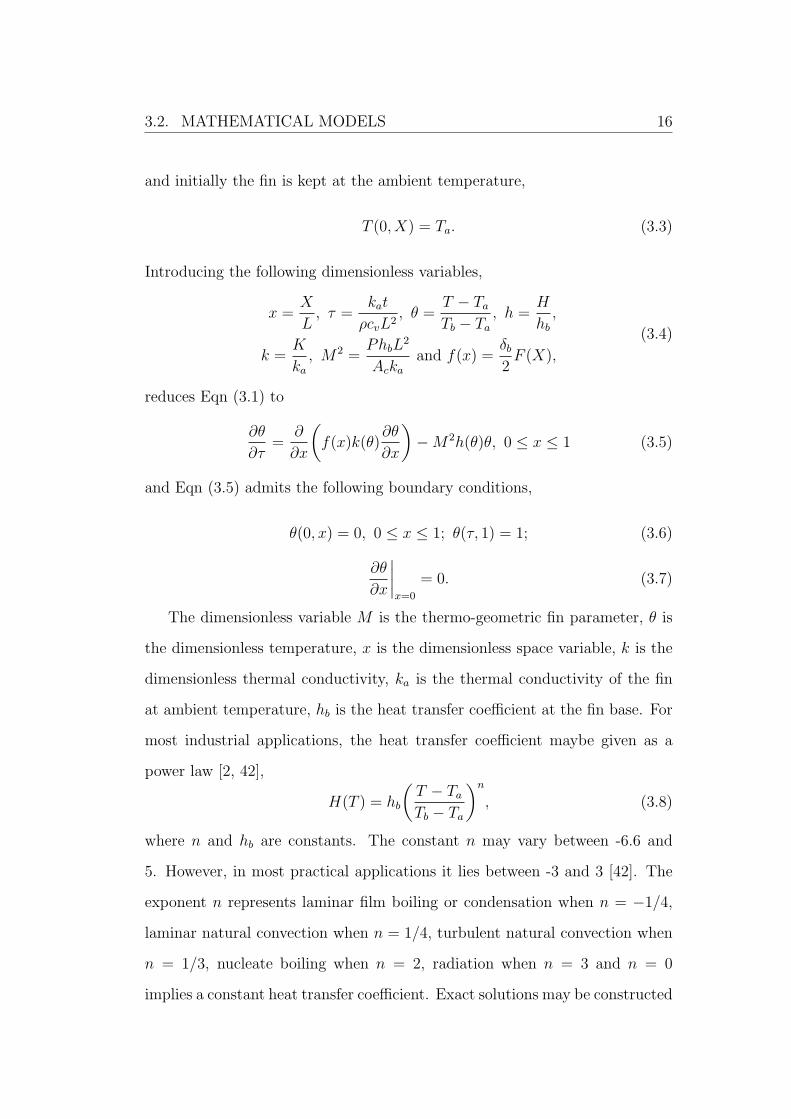
Case (n,m) = (2, 3)
θ(x) = a+M2
2x2 − M4
4ax4 +
M6
4a2x6 − 33M8
122a3x8 +
127M10
336a4x10
− 1889M12
3696a5x12 +
160649M14
224224a6x12 − 7225M16
7007a7x16 + . . . . (4.37)
Case (n,m) = (3, 2)
θ(x) = a+a2M2
2x2 − a3M4
12x4 +
29a4M6
360x6 − 307a5M8
5040x8
+23483a6M10
453600x10 − 125893a7M12
2721600x12 +
1635899a8M14
38102400x14
− 23417113a9M16
571536000x16 + . . . . (4.38)
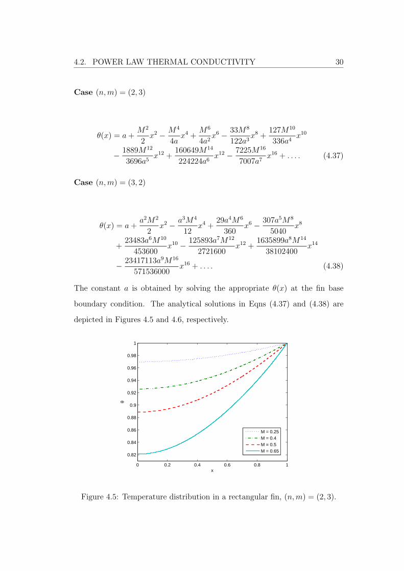
The constant a is obtained by solving the appropriate θ(x) at the fin base
boundary condition. The analytical solutions in Eqns (4.37) and (4.38) are
depicted in Figures 4.5 and 4.6, respectively.
0 0.2 0.4 0.6 0.8 1
0.82
0.84
0.86
0.88
0.9
0.92
0.94
0.96
0.98
1
x
θ
M = 0.25M = 0.4M = 0.5M = 0.65
Figure 4.5: Temperature distribution in a rectangular fin, (n,m) = (2, 3).

4.2. POWER LAW THERMAL CONDUCTIVITY 31
0 0.2 0.4 0.6 0.8 1
0.84
0.86
0.88
0.9
0.92
0.94
0.96
0.98
1
x
θ
M = 0.25M = 0.4M = 0.5M = 0.65
Figure 4.6: Temperature distribution in a rectangular fin, (n,m) = (3, 2).
(iii) The convex profile and power law thermal conductivity
In this section we present solutions for the equation describing the heat transfer
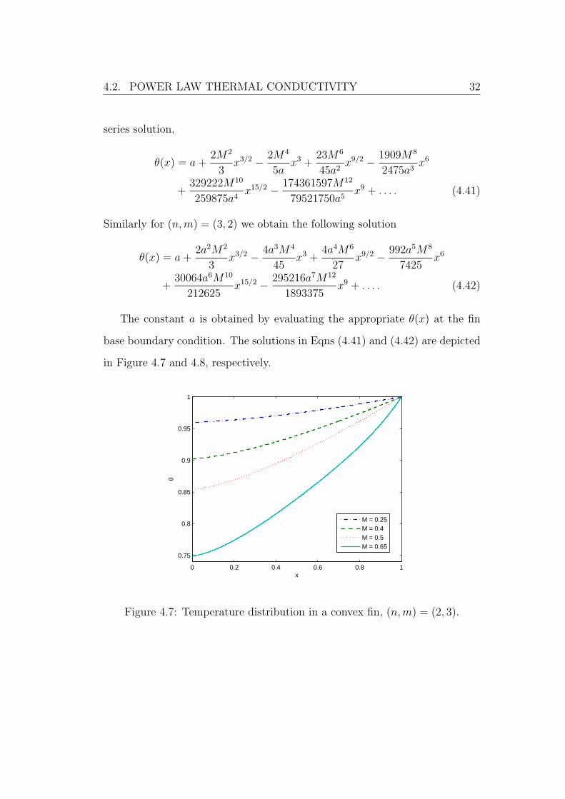
in a fin with convex parabolic profile and power law thermal conductivity. We
consider Eqn (4.2), with the definition y = x1/2. Here we consider the values
{(n,m) = (2, 3); (3, 2)} . With (n,m) = (2, 3), Eqn (4.2) reduces to
d
dy
[θ3dθ
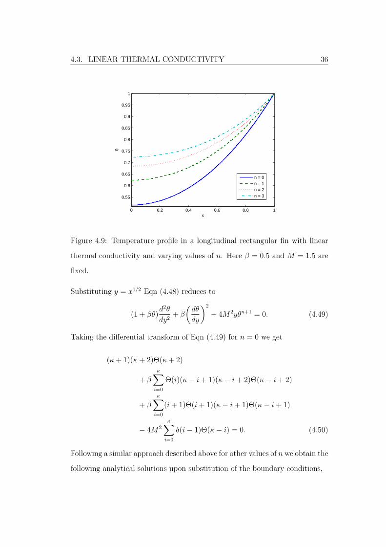
dy
]− 4M2yθ3 = 0. (4.39)
Taking the differential transform of Eqn (4.39) we obtain the following relation
κ∑i=0
κ−i∑l=0
κ−i−l∑p=0
[Θ(p)Θ(l)Θ(i)(κ− i− l − p+ 1)(κ− i− l − p+ 2)×
Θ(κ− i− l − p+ 2) + 3Θ(p)Θ(l)(i+ 1)Θ(i+ 1)×
(κ− i− l − p+ 1)Θ(κ− i− l − p+ 1)
− 4M2δ(p− 1)Θ(l)Θ(i)Θ(κ− i− l − p)
]= 0, (4.40)
and substituting the transformed boundary conditions, we obtain the following
4.2. POWER LAW THERMAL CONDUCTIVITY 32
series solution,
θ(x) = a+2M2
3x3/2 − 2M4
5ax3 +
23M6
45a2x9/2 − 1909M8
2475a3x6
+329222M10
259875a4x15/2 − 174361597M12
79521750a5x9 + . . . . (4.41)
Similarly for (n,m) = (3, 2) we obtain the following solution
θ(x) = a+2a2M2
3x3/2 − 4a3M4
45x3 +
4a4M6
27x9/2 − 992a5M8
7425x6
+30064a6M10
212625x15/2 − 295216a7M12
1893375x9 + . . . . (4.42)
The constant a is obtained by evaluating the appropriate θ(x) at the fin
base boundary condition. The solutions in Eqns (4.41) and (4.42) are depicted
in Figure 4.7 and 4.8, respectively.
0 0.2 0.4 0.6 0.8 1
0.75
0.8
0.85
0.9
0.95
1
x
θ
M = 0.25M = 0.4M = 0.5M = 0.65
Figure 4.7: Temperature distribution in a convex fin, (n,m) = (2, 3).

4.3. LINEAR THERMAL CONDUCTIVITY 33
0 0.2 0.4 0.6 0.8 1
0.82
0.84
0.86
0.88
0.9
0.92
0.94
0.96
0.98
1
x
θ
M = 0.25M = 0.4M = 0.5M = 0.65
Figure 4.8: Temperature distribution in a convex fin, (n,m) = (3, 2).
4.3 Linear thermal conductivity
In many engineering applications and many materials, thermal conductivity
depends linearly on temperature (See e.g [48])
4.3.1 The rectangular profile, f(x) = 1
In this section we present solutions for the equation representing the heat
transfer in a fin with rectangular profile and thermal conductivity depending
linearly on temperature. That is, we consider Eqn (3.11) with f(x) = 1 and
k(θ) = 1+ βθ. With these properties, taking the differential transform of Eqn
(3.11) for n = 0 we get
(κ+ 1)(κ+ 2)Θ(κ+ 2)
+ β
κ∑i=0
[Θ(i)(κ− i+ 1)(κ− i+ 2)Θ(κ− i+ 2)
+ β
κ∑i=0
(i+ 1)Θ(i+ 1)(κ− i+ 1)Θ(κ− i+ 1)]−M2Θ(κ) = 0. (4.43)

4.3. LINEAR THERMAL CONDUCTIVITY 34
Following a similar approach described above for other values of n we obtain the
following analytical solutions upon substitution of the boundary conditions,
Case n = 0
θ(x) = a+M2a
2(1 + βa)x2 − M4a(−1 + 2βa)
24(1 + βa)3x4 +
M6a(1− 16βa+ 28β2a2)
720(1 + βa)5x6
− M8a(−1 + 78βa− 600β2a2 + 896β3a3)
40320(1 + βa)7x8
+M10a(1− 332βa+ 7812β2a2 − 39896β3a3 + 51184β4a4)
3628800(1 + βa)9x10
+ . . . . (4.44)
Case n = 1
θ(x) = a+M2a2
2(1 + βa)x2 − M4a3(−1 + 2βa)
24(1 + βa)3x4
+M6a4(10− 16βa+ 19β2a2)
720(1 + βa)5x6
− M8a5(−80 + 342βa− 594β2a2 + 559β3a3)
40320(1 + βa)7x8
+M10a6(1000− 7820βa+ 24336β2a2 − 36908β3a3 + 29161β4a4)
3628800(1 + βa)9x10
+ . . . . (4.45)

4.3. LINEAR THERMAL CONDUCTIVITY 35
Case n = 2
θ(x) = a+M2a3
2(1 + βa)x2 +
M4a5
8(1 + βa)3x4 +
M6a7(3 + 2β2a2)
80(1 + βa)5x6
+M8a9(49− 20βa+ 66β2a2 − 40β3a3)
4480(1 + βa)7x8
+M10a11(427− 440βa+ 1116β2a2 − 1020β3a3 + 672β4a4)
134400(1 + βa)9x10
+ . . . . (4.46)
Case n = 3
θ(x) = a+M2a4
2(1 + βa)x2 +
M4a7(4 + βa)
24(1 + βa)3x4 +
M6a10(52 + 32βa+ 25β2a2)
720(1 + βa)5x6
+M8a13(1288 + 1020βa+ 1212β2a2 − 95β3a3)
40320(1 + βa)7x8
+M10a16(52024 + 45688βa+ 77184β2a2 − 680β3a3 + 15025β4a4)
3628800(1 + βa)9x10
+ . . . . (4.47)
The constant a may be obtained from the boundary condition on the appro-
priate solution. The solutions in Eqns (4.44), (4.45), (4.46) and (4.47) are
depicted in Figure 4.9.
4.3.2 The convex parabolic profile, f(x) = x1/2
In this section we present solutions for the equation describing the heat transfer
in a fin with convex parabolic profile and the thermal conductivity depending
linearly on temperature. That is, we consider Eqn (4.2) with k(θ) = 1 + βθ
and f(x) = x1/2,
d
dx
[x1/2(1 + βθ)
dθ
dx
]−M2θn+1 = 0. (4.48)
4.3. LINEAR THERMAL CONDUCTIVITY 36
0 0.2 0.4 0.6 0.8 1
0.55
0.6
0.65
0.7
0.75
0.8
0.85
0.9
0.95
1
x
θ
n = 0n = 1n = 2n = 3
Figure 4.9: Temperature profile in a longitudinal rectangular fin with linear
thermal conductivity and varying values of n. Here β = 0.5 and M = 1.5 are
fixed.
Substituting y = x1/2 Eqn (4.48) reduces to
(1 + βθ)d2θ
dy2+ β
(dθ
dy
)2
− 4M2yθn+1 = 0. (4.49)
Taking the differential transform of Eqn (4.49) for n = 0 we get
(κ+ 1)(κ+ 2)Θ(κ+ 2)
+ βκ∑
i=0
Θ(i)(κ− i+ 1)(κ− i+ 2)Θ(κ− i+ 2)
+ βκ∑
i=0
(i+ 1)Θ(i+ 1)(κ− i+ 1)Θ(κ− i+ 1)
− 4M2
κ∑i=0
δ(i− 1)Θ(κ− i) = 0. (4.50)
Following a similar approach described above for other values of n we obtain the
following analytical solutions upon substitution of the boundary conditions,

4.3. LINEAR THERMAL CONDUCTIVITY 37
Case n = 0
θ(x) = a+2M2c
3(1 + βa)x3/2 − 2M4a(−2 + 3βa)
45(1 + βa)3x3
+M6a(2− 25βa+ 33β2a2)
405(1 + βa)5x9/2
− M8a(−10 + 599βa− 3582β2a2 + 4059β3a3)
66825(1 + βa)7x6 + . . . . (4.51)
Case n = 1
θ(x) = a+2M2a2
3(1 + βa)x3/2 − 2M4a3(−4 + βa)
45(1 + βa)3x3
+2M6a4(9− 11βa+ 10β2a2)
405(1 + βa)5x9/2
− 2M8a5(−330 + 1118βa− 1584β2a2 + 1093β3a3)
66825(1 + βa)7x6 + . . . . (4.52)
Case n = 2
θ(x) = a+2M2a3
3(1 + βa)x3/2 +
2M4a5(6 + βa)
45(1 + βa)3x3
+M6a7(16 + 3βa+ 7β2a2)
135(1 + βa)5x9/2
+M8a9(1160− 107βa+ 1116β2a2 − 367β3a3)
22275(1 + βa)7x6 + . . . . (4.53)

4.3. LINEAR THERMAL CONDUCTIVITY 38
Case n = 3
θ(x) = a+2M2a4
3(1 + βa)x3/2 +
2M4a7(8 + 3βa)
45(1 + βa)3x3
+4M6a10(23 + 17βa+ 9β2a2)
405(1 + βa)5x9/2
+2M8a13(5000 + 4868βa+ 4356β2a2 + 363β3a3)
66825(1 + βa)7x6 + . . . . (4.54)
The constant a may be obtained from the boundary condition on the ap-
propriate θ(x). The solutions in Eqns (4.51), (4.52), (4.53) and (4.54) are
depicted in Figure 4.10.
0 0.2 0.4 0.6 0.8 1
0.5
0.6
0.7
0.8
0.9
1
x
θ
n = 0n = 1n = 2n = 3
Figure 4.10: Temperature profile in a longitudinal convex parabolic fin with
linear thermal conductivity and varying values of n. Here β = 0.5 andM = 1.5
are fixed.

4.3. LINEAR THERMAL CONDUCTIVITY 39
4.3.3 The exponential profile, f(x) = eσx
In this section we present solutions for the heat transfer equation in a fin with
exponential profile and thermal conductivity depending linearly on tempera-
ture. That is, we consider Eqn (3.11) with k(θ) = 1 + βθ and f(x) = eσx,
where σ is a constant,
d
dx
[eσx(1 + βθ)
dθ
dx
]−M2θn+1 = 0. (4.55)
Taking the differential transform of Eqn (4.55) for n = 0 we obtain the follow-
ing recurrence relation;
κ∑i=0
σi
i!(κ− i+ 1)(κ− i+ 2)Θ(κ− i+ 2)
+ βκ∑
i=0
κ−i∑t=0
σt
t!(κ− i− t+ 1)(κ− i− t+ 2)Θ(κ− i− t+ 2)
+ σκ∑
i=0
σi
i!(κ− i+ 1)Θ(κ− i+ 1)
+ σβ
κ∑i=0
κ−i∑t=0
σi
i!(κ− i− t+ 1)Θ(i)Θ(κ− i− t+ 1)
+ βκ∑
i=0
κ−i∑t=0
σi
i!(i+ 1)(κ− i− t+ 1)Θ(i+ 1)Θ(κ− i− t+ 1)
−M2Θ(κ) = 0. (4.56)
Following a similar approach described above for other values of n we obtain the
following analytical solutions upon substitution of the boundary conditions,

4.3. LINEAR THERMAL CONDUCTIVITY 40
Case n = 0
θ(x) = a+M2a
2(1 + βa)x2 − σM2a(2 + βa+ β2a)
6(1 + βa)2x3
+M2a(M2(1− 2β2a) + σ2(3 + 3βa+ β3a2 + β4a2 + β2a(3 + a)))
24(1 + βa)3x4
+ . . . . (4.57)
Case n = 1
θ(x) = a+M2a2
2(1 + βa)x2 − σM2a2(2 + βa+ β2a)
6(1 + βa)2x3
+M2a2(M2a(2 + βa− 2β2a) + σ2(3 + 3βa+ β3a2 + β4a2 + β2a(3 + a)))
24(1 + βa)3x4
+ . . . . (4.58)
Case n = 2
θ(x) = a+M2a3
2(1 + βa)x2 − σM2a3(2 + βa+ β2a)
6(1 + βa)2x3
+M2a3(M2a2(3 + 2βa− 2β2a) + σ2(3 + βa(3 + β2a+ β3a+ β(3 + a))))
24(1 + βa)3x4
+ . . . . (4.59)

4.3. LINEAR THERMAL CONDUCTIVITY 41
Case n = 3
θ(x) = a+M2a4
2(1 + βa)x2 − σM2a4(2 + βa+ β2a))
6(1 + βa)2x3
+M2a4(M2a3(4 + 3βa− 2β2a) + σ2(3 + βa(3 + β2a+ β3a+ β(3 + a))))
24(1 + βa)3x4
+ . . . . (4.60)
The constant a may be obtained from the boundary condition on the appropri-
ate θ(x). The solutions in Eqns (4.57), (4.58), (4.59) and (4.60) are depicted
in Figure 4.11.
0 0.2 0.4 0.6 0.8 1
0.7
0.75
0.8
0.85
0.9
0.95
1
x
θ
n = 0n = 1n = 2n = 3
Figure 4.11: Temperature profile in a longitudinal fin of exponential profile
with linear thermal conductivity and varying values of n. Here β = 0.5 and
M = 1.5 are fixed.

4.4. FIN EFFICIENCY AND HEAT FLUX 42
4.4 Fin efficiency and heat flux
4.4.1 Fin efficiency
The heat transfer rate from a fin is given by Newton’s second law of cooling,
Q =
∫ L
0
PH(T )(T − Ta)dx. (4.61)
Fin efficiency is defined as the ratio of the fin heat transfer rate to the rate
that would be if the entire fin were at the base temperature and is given by
(see e.g. [1])
η=Q
Qideal
=
∫ L
0PH(T )(T − Ta)dX
PhbL(Tb − Ta). (4.62)
In dimensionless variables we have
η =
∫ 1
0
θn+1dx. (4.63)
We consider the solutions (4.44), (4.45), (4.46) and (4.47) and depict the fin
efficiency (4.63) in Figure 4.12.
0 0.5 1 1.5 20.55
0.6
0.65
0.7
0.75
0.8
0.85
0.9
0.95
1
M
η
n = 0n = 1n = 2n = 3
Figure 4.12: Fin efficiency of a longitudinal rectangular fin. Here β = 0.75..
4.5. DISCUSSION OF RESULTS 43
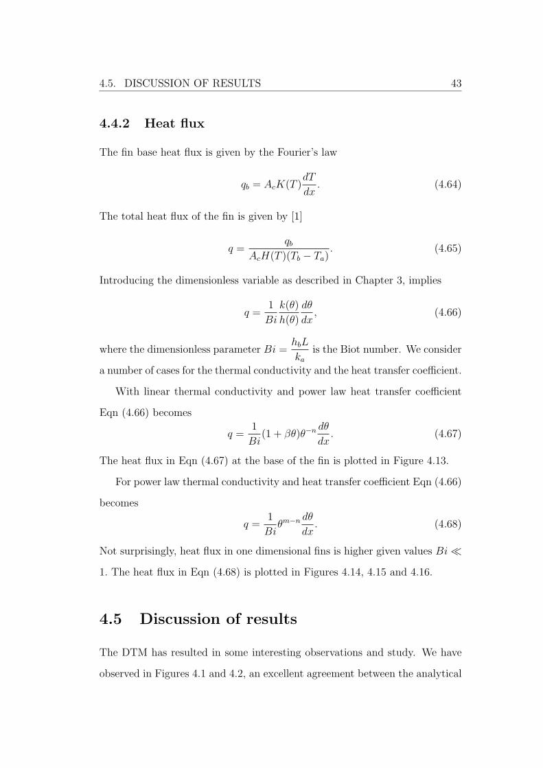
4.4.2 Heat flux
The fin base heat flux is given by the Fourier’s law
qb = AcK(T )dT
dx. (4.64)
The total heat flux of the fin is given by [1]
q =qb
AcH(T )(Tb − Ta). (4.65)
Introducing the dimensionless variable as described in Chapter 3, implies
q =1
Bi
k(θ)
h(θ)
dθ
dx, (4.66)
where the dimensionless parameter Bi =hbL
kais the Biot number. We consider
a number of cases for the thermal conductivity and the heat transfer coefficient.
With linear thermal conductivity and power law heat transfer coefficient
Eqn (4.66) becomes
q =1
Bi(1 + βθ)θ−n dθ
dx. (4.67)
The heat flux in Eqn (4.67) at the base of the fin is plotted in Figure 4.13.
For power law thermal conductivity and heat transfer coefficient Eqn (4.66)
becomes
q =1
Biθm−n dθ
dx. (4.68)
Not surprisingly, heat flux in one dimensional fins is higher given values Bi ≪
1. The heat flux in Eqn (4.68) is plotted in Figures 4.14, 4.15 and 4.16.
4.5 Discussion of results
The DTM has resulted in some interesting observations and study. We have
observed in Figures 4.1 and 4.2, an excellent agreement between the analytical

4.5. DISCUSSION OF RESULTS 44
0 0.5 1 1.5 20
5
10
15
20
25
M
q
n = 0n = 1n = 2n = 3
Figure 4.13: Base heat flux in a longitudinal rectangular fin with linear thermal
conductivity. Here β = 0.1..
0 0.2 0.4 0.6 0.8 1−5
0
5
10
15
20
25
30
35
40
45
x
q
M = 0.25M = 0.4M = 0.5M = 0.65
Figure 4.14: Heat flux across a longitudinal rectangular fin with power law
thermal conductivity. Here n−m > 0, Bi = 0.01..

4.5. DISCUSSION OF RESULTS 45
0 0.2 0.4 0.6 0.8 10
5
10
15
20
25
30
x
q
M = 0.25M = 0.4M = 0.5M = 0.65
Figure 4.15: Heat flux across a longitudinal rectangular fin with power law
thermal conductivity. Here n−m < 0, Bi = 0.01..
0 0.2 0.4 0.6 0.8 10
5
10
15
20
25
30
35
x
q
M = 0.25M = 0.4M = 0.5M = 0.65
Figure 4.16: Base heat flux in a longitudinal rectangular fin with power law
thermal conductivity. Here n−m = 0, Bi = 0.01..
4.5. DISCUSSION OF RESULTS 46
solutions generated by DTM and the exact solution obtained in [5]. In par-
ticular, we considered a fin problem in which both thermal conductivity and
heat transfer coefficient are both given by the same power law. Furthermore,
we notice from Table 4.1 that an absolute error of approximately 3.5e − 005
is produced by DTM of order O(15). In Table 4.2 an absolute error of ap-
proximately 6.5e− 006 is produced for the same order. This confirms that the
DTM converges faster and can provide accurate results with minimum com-
putational effort. As such, a tremendous confidence in the DTM in terms of
the accuracy and effectiveness was built and thus we used this method to solve
other problems for which exact solutions are harder to construct.
In the Figures 4.3, 4.4, 4.5, 4.6, 4.7 and 4.8, we observe that the fin tem-
perature increases with the decreasing values of the thermo-geometric fin pa-
rameter. Here, the values of the exponents are fixed. Also, we observe that
fin temperature is higher when n −m > 0, that is, when heat transfer coeffi-
cient is higher than the thermal conductivity. We observe in Figures 4.9, 4.10
and 4.11, that the fin temperature increases with the increasing values of n.
Furthermore, it appears that the fin with exponential profile performs least
in transferring the heat from the base, since the temperature in such a fin is
much higher than that of the rectangular and the convex parabolic profiles. In
other words, heat dissipation to the fluid surrounding the extended surface is
much faster in longitudinal fins of rectangular and convex parabolic profiles.
In Figure 4.12, fin efficiency decreases with increasing thermo-geometric fin
parameter. Also, fin efficiency increases with increasing values of n. It is easy
to show that the thermo-geometric fin parameter is directly proportional to
the aspect ratio (extension factor) with square root of the Biot number be-
ing the proportionality constant. As such shorter fins are more efficient than
longer ones. The increased Biot number results in less efficient fin whenever

4.5. DISCUSSION OF RESULTS 47
the space is confined, that is where the length of the fin cannot be increased.
Figure 4.13, depicts the heat flux at the fin base. The amount of heat en-
ergy dissipated from the fin base is of immense interest in engineering [49].
We observe in Figure 4.13 that the base heat flux increases with the thermo-
geometric fin parameter for considered values of the exponent n (see also [49]).
Figures 4.14, 4.15 and 4.16 display the heat flux across the fin length. We note
that the heat flux across the fin length increases with increasing values of the
thermo-geometric fin parameter.
The performance of fins is sometimes expressed in terms of the fin effec-
tiveness ε defined as [50],
ε =q
AcH(T )(Tb − Ta), (4.69)
where Ac is cross sectional area at the fin base. q represents the rate of heat
transfer from this area if no fins are attached to the surface. Fin effectiveness
is then the ratio of the fin heat transfer rate to the heat transfer rate of the
object if it had no fin. The physical significance of effectiveness of fin can be
summarized below
◦ An effectiveness of ε = 1 indicates that the addition of a fin to the surface
does not affect heat transfer at all. That is, heat conducted to the fin
through the base area Ac is equal to the heat transferred from the same
area Ac to the surrounding medium.
◦ An effectiveness of ε < 1 indicates that the fin actually acts as an insula-
tion, slowing down the heat transfer from the surface. This situation can
occur when fins made of low thermal conductivity materials are used.
◦ An effectiveness of ε > 1 indicates that the fins are enhancing heat
transfer from the surface, as they should. However, the use of fins cannot

4.6. CONCLUDING REMARKS 48
be justified unless ε is sufficiently larger than 1. Finned surfaces are
designed on the basis of maximizing effectiveness of a specified cost or
minimizing cost for a desired effectiveness.
4.6 Concluding remarks
In this chapter we have successfully applied the 1D DTM to highly nonlinear
problems arising in heat transfer through longitudinal fins of various profiles.
Both thermal conductivity and heat transfer coefficient are given as functions
of temperature. The DTM agreed well with exact solutions when the thermal
conductivity and heat transfer coefficient are given by the same power law. A
rapid convergence to the exact solution was observed. Following the confidence
in DTM built by the results mentioned, we then solved various problems.
Obtained results have been shown in tables and figures listed in this chapter.
The results obtained in this chapter are significant improvements on the
known results. In particular, both the heat transfer coefficient and thermal
conductivity are allowed to be given by the power law functions of temperature,
and also we considered three fin profiles. We note that exact solutions are
difficult if not impossible to construct when the exponents of the power laws
for the heat transfer coefficient and thermal conductivity are distinct.

Chapter 5
Application of the 2D DTM to
transient heat transfer problems
5.1 Introduction
In this Chapter we extend the 1D DTM in order to solve partial differen-
tial equations. The resulting method is referred to as the 2D DTM. We saw
from the previous chapter that the differential transform method offers great
advantages of straightforward applicability, computational efficiency and high
accuracy. In the following sections we attempt to solve transient heat conduc-
tion equation where the thermal conductivity is given by a linear function of
temperature. We consider heat transfer in fins of convex parabolic profile and
the rectangular profile. Using 2D DTM to solve PDEs consists of three main
steps which are; transforming the PDE into algebraic equations, solving the
equations, and inverting the solution of algebraic equations to obtain a series
solution or an approximate solution.
When thermal conductivity depends linearly on temperature, Eqn (3.5) is
49

5.2. RECTANGULAR PROFILE 50
then given by the following nonlinear equation,
∂θ
∂τ=
∂
∂x
(f(x)(1 + βθ)
∂θ
∂x
)−M2θn+1 (5.1)
The initial condition is,
θ(0, x) = 0, 0 ≤ x ≤ 1, (5.2)
the boundary conditions are,
θ(τ, 1) = 1, (5.3)
and
∂θ
∂x
∣∣∣∣x=0
= 0. (5.4)
5.2 Rectangular profile
Here we consider a fin of a rectangular profile f(x) = 1 for transient heat
conduction through fins.
5.2.1 Solution for n = 1
Taking the two-dimensional differential transform of eqn (5.1) with f(x) = 1
and n = 1, we obtain the following recurrence relation
(k + 1)Θ(k + 1, h) = (h+ 1)(h+ 2)Θ(k, h+ 2)
+ βκ∑
i=0
h∑j=0
Θ(κ− i, j)(h+ 1− j)(h+ 2− j)Θ(i, h+ 2− j)
+ βκ∑
i=0
h∑j=0
(j + 1)Θ(κ− i, j + 1)(h+ 1− j)Θ(i, h+ 1− j)
−M2
κ∑i=0
h∑j=0
Θ(i, h− j)Θ(κ− i, j), (5.5)
5.2. RECTANGULAR PROFILE 51
where Θ(κ, h) is the differential transform of θ(τ, x).
Taking the two-dimensional differential transform of the initial condition
(5.2) and boundary condition (5.4) we obtain the following transformations
respectively,
Θ(0, h) = 0, h = 0, 1, 2, . . . (5.6)
Θ(κ, 1) = 0, κ = 0, 1, 2, . . . . (5.7)
We consider the other boundary condition as follows,
Θ(κ, 0) = a, a ∈ R, κ = 1, 2, 3, . . . (5.8)
where the constant a can be determined from the boundary condition (5.7) at
each time step after obtaining the series solution.
Substituting Eqns (5.6)-(5.8) into (5.5) we obtain the following,
Θ(1, 2) = a (5.9)
Θ(2, 2) =1
2(3a− 2βa2 + a2M2) (5.10)
Θ(3, 2) =1
2(4a− 5βa2 + 2β2a3 + 2a2M2 − βa3M2) (5.11)
Θ(1, 4) =1
12(3a− 2βa2 + a2M2) (5.12)
Θ(2, 4) =1
24(12a− 33βa2 + 10β2a3 + 10a2M2 − 5βa3M2) (5.13)
...
Substituting Eqns (5.6)-(5.13) into (2.9) we obtain the following series so-
lution,
θ(τ, x) = aτ + aτ 2 + aτx2 +1
2(3a− 2βa2 + a2M2)τ 2x2
+ aτ 3 +1
2(4a− 5βa2 + 2β2a3 + 2a2M2 − βa3M2)τ 3x2
+ aτ 4 +1
12(3a− 2βa2 + a2M2)τx4
+1
24(12a− 33βa2 + 10β2a3 + 10a2M2 − 5βa3M2)τ 2x4 + . . . (5.14)

5.2. RECTANGULAR PROFILE 52
The constant a can be determined from the boundary condition (5.2) at
each time step. To obtain the value of a, we substitute the boundary condition
(5.2) into (5.14) at the point x = 1. Thus, we have,
θ(τ, 1) = aτ + aτ 2 + aτ +1
2(3a− 2βa2 + a2M2)τ 2
+ aτ 3 +1
2(4a− 5βa2 + 2β2a3 + 2a2M2 − βa3M2)τ 3
+ aτ 4 +1
12(3a− 2βa2 + a2M2)τ
+1
24(12a− 33βa2 + 10β2a3 + 10a2M2 − 5βa3M2)τ 2
+ . . . = 1 (5.15)
We then obtain the expression for θ(τ, x) upon substituting the obtained
value of a into equation (5.14). Using the first 40 terms of the power series
solution we plot the solution (5.14) for various parameters as shown in Figures
5.1,5.2 and 5.3.
5.2.2 Solution for n = 0
θ(τ, x) = aτ + aτ 2 +1
2(2a+ aM2)τx2 +
1
2(3a− 2a2β + aM2 − a2βM2)τ 2x2
+ aτ 3 +1
2(4a− 5a2β + 2a3β2 + aM2 − 2a2βM2 + a3β2M2)τ 3x2
+ aτ 4 +1
24(6a− 4a2β + 4aM2 − 2a2βM2 + aM4)τx4 + . . . (5.16)

5.3. CONVEX PARABOLIC PROFILE 53
5.2.3 Solution for n = 2
θ(τ, x) = aτ + aτ 2 + aτx2 +1
2(3a− 2a2β)τ 2x2 + aτ 3
+1
2(4a− 5a2β + 2a3β2 + a3M2)τ 3x2 + aτ 4
+1
12(3a− 2a2β)τx4 +
1
24(12a− 33a2β + 10a3β2 + 3a3M2)τ 2x4 + . . . .
(5.17)
5.2.4 Solution for n = 3
θ(τ, x) = aτ + aτ 2 + aτx2 +1
2(3a− 2a2β)τ 2x2 + aτ 3
+1
2(4a− 5a2β + 2a3β2)τ 3x2 + aτ 4 +
1
12(3a− 2a2β)τx4
+1
24(12a− 33a2β + 10a3β2)τ 2x4 + . . . (5.18)
Plots of solutions (5.16), (5.17) and (5.18) for various parameters are shown
in Figures 5.4-5.8.
5.3 Convex parabolic profile
Here we consider a fin of a convex profile f(x) = x1/2 for transient heat con-
duction through fins. We make a substitution y = x1/2 to eliminate fractional
powers. Eqn (5.1) then simplifies to
4y∂θ
∂τ= (1 + βθ)
∂2θ
∂y2+ β
(∂θ
∂y
)2
− 4M2yθn+1 (5.19)

5.3. CONVEX PARABOLIC PROFILE 54
5.3.1 Solution for n = 1
Taking the two-dimensional differential transform of eqn (5.19) for n = 1, we
obtain
4κ∑
i=0
h∑j=0
(i+ 1)Θ(i+ 1, h− j)δ(j − 1)δ(k − i) = (h+ 1)(h+ 2)Θ(k, h+ 2)
+ β
κ∑i=0
h∑j=0
Θ(κ− i, j)(h+ 1− j)(h+ 2− j)Θ(i, h+ 2− j)
+ βκ∑
i=0
h∑j=0
(j + 1)Θ(κ− i, j + 1)(h+ 1− j)Θ(i, h+ 1− j)
− 4M2
κ∑i=0
k−i∑t=0
h∑j=0
h−j∑p=0
Θ(i, h− j − p)Θ(t, j)δ(κ− i− t)δ(p− 1) (5.20)
Substituting Eqns (5.6)-(5.8) into Eqn (5.20) we obtain the following,
Θ(1, 3) =4a
3(5.21)
Θ(2, 3) = −2
3(−3a+ 2a2β − a2M2) (5.22)
Θ(3, 3) =2
3(4a− 5a2β + 2a3β2 + 2a2M2 − a3βM2) (5.23)
Θ(4, 3) = −2
3(−5a+9a2β−7a3β2+2a4β3−3a2M2+3a3βM2−a4β2M2) (5.24)
...
Substituting Eqns (5.6)-(5.8) and Eqns (5.21)-(5.24) into Eqn (2.9) we ob-
tain the following series solution,
θ(τ, x) = aτ + aτ 2 +4a
3τx3/2 − 2a
3(−3 + 2aβ − aM2)τ 2x3/2 + aτ 3
+2a
3(4− 5aβ + 2a2β2 + 2aM2 − a2βM2)τ 3x3/2 + aτ 4 + . . . . (5.25)

5.4. DISCUSSION OF RESULTS 55
5.3.2 Solution for n = 0
θ(τ, x) = aτ + aτ 2 +2a
3(2 +M2)τx3/2 − 2a
3(−3 + 2aβ −M2 + aβM2)τ 2x3/2
+2a
3(4− 5aβ + 2a2β2 +M2 − 2aβM2 + a2β2M2)τ 3x3/2 + aτ 3 + . . . .
(5.26)
5.3.3 Solution for n = 2
θ(τ, x) = aτ + aτ 2 +4a
3τx3/2 − 2a
3(−3 + 2aβ − aM2)τ 2x3/2 + aτ 3
+2a
3(4− 5aβ + 2a2β2 + 2aM2 − a2βM2)τ 3x3/2 + aτ 4 + . . . . (5.27)
Plots of solutions (5.25) and (5.27) are shown in Figures 5.9 and 5.10 respec-
tively.
5.4 Discussion of results
Some interesting results were obtained using the 2D DTM. We observe in Fig-
ure 5.1 that the fin temperature increases with time. This transient tempera-
ture profile approaches the steady state solution as time evolves. We observe
in Figures 5.2 and 5.9 that the temperature decreases with increasing values
of the thermo-geometric fin parameter. We note that the thermo-geometric fin
parameter M = (Bi)1/2E, where Bi = hbδ/ka is the Biot number and E = L/δ
is the aspect ratio or the extension factor. Evidently, small values of M cor-
responds to the relatively short and thick fins of high conductivity and high
values of M correspond to longer and thin fins of poor conductivity [48]. A fin
is an excellent dissipater at small values of M. As M increases the convective

5.4. DISCUSSION OF RESULTS 56
0 0.2 0.4 0.6 0.8 10.1
0.2
0.3
0.4
0.5
0.6
0.7
0.8
0.9
1
x
θ
τ = 0.1
τ = 0.2
τ = 1.2steady state
Figure 5.1: Transient temperature distribution in a rectangular fin with linear
thermal conductivity, n = 1, β = 1,M = 6.
0 0.2 0.4 0.6 0.8 10
0.1
0.2
0.3
0.4
0.5
0.6
0.7
0.8
0.9
1
x
θ
M = 0.25M = 10M = 40M = 100
Figure 5.2: Transient temperature distribution in a rectangular fin with linear
thermal conductivity, n = 1, β = 1, τ = 1.2.

5.4. DISCUSSION OF RESULTS 57
0 0.2 0.4 0.6 0.8 10
0.1
0.2
0.3
0.4
0.5
0.6
0.7
0.8
0.9
1
x
θ
β = 1
β = 3
β = 5
β = 7
Figure 5.3: Transient temperature distribution in a rectangular fin with linear
thermal conductivity, n = 1,M = 2.5, τ = 1.2.
0 0.2 0.4 0.6 0.8 10
0.1
0.2
0.3
0.4
0.5
0.6
0.7
0.8
0.9
1
x
θ
M = 0.25M = 10M = 40
Figure 5.4: Transient temperature distribution in a rectangular fin with linear
thermal conductivity, n = 0, β = 1, τ = 1.2.

5.4. DISCUSSION OF RESULTS 58
0 0.2 0.4 0.6 0.8 10
0.1
0.2
0.3
0.4
0.5
0.6
0.7
0.8
0.9
1
x
θ
n = 0n = 1n = 2n = 3
Figure 5.5: Transient temperature distribution in a rectangular fin with linear
thermal conductivity, M = 40, β = 1, τ = 1.2.
0 0.05 0.1 0.15 0.2 0.25 0.3 0.35 0.4 0.450
0.1
0.2
0.3
0.4
0.5
0.6
0.7
0.8
0.9
1
τ
θ
x=0.75x=0.85x=0.95
Figure 5.6: Transient temperature distribution in a rectangular fin with linear
thermal conductivity, M = β = n = 1.

5.4. DISCUSSION OF RESULTS 59
00.2
0.40.6
0.81
0
0.1
0.2
0.3
0
0.2
0.4
0.6
0.8
1
xτ
θ
Figure 5.7: Transient temperature distribution in a rectangular fin with linear
thermal conductivity, M = β = n = 1.
0 0.05 0.1 0.15 0.2 0.25 0.3 0.35 0.40
0.1
0.2
0.3
0.4
0.5
0.6
0.7
0.8
0.9
1
τ
θ
Figure 5.8: Transient temperature distribution in a rectangular fin with linear
thermal conductivity, M = 0.75, β = 1, n = 1.

5.4. DISCUSSION OF RESULTS 60
0 0.2 0.4 0.6 0.8 10
0.1
0.2
0.3
0.4
0.5
0.6
0.7
0.8
0.9
1
x
θ
M = 10M = 5M = 0.75
Figure 5.9: Transient temperature distribution in a convex parabolic fin with
linear thermal conductivity, β = 1, τ = 0.2.
0 0.2 0.4 0.6 0.8 10.1
0.2
0.3
0.4
0.5
0.6
0.7
0.8
0.9
1
x
θ
Convex parabolic profileRectangular profile
Figure 5.10: Transient temperature distribution in a rectangular and convex
parabolic fin with linear thermal conductivity, n = 2,M = 6, β = 1, τ = 1.2.
5.4. DISCUSSION OF RESULTS 61
heat loss increases and the temperature profile becomes steeper reflecting high
base heat flow rates (see e.g. [51]).
We observe in Figure 5.6, that the closer one gets to the base of the fin,
the initial temperature gets to unity, even at small time scale and this cor-
respond to the imposed initial condition. In Figure 5.3, we observe that the
temperature in the fin increases with the increasing values of the thermal con-
ductivity gradient. We note that β = 0 implies that the thermal conductivity
is a constant given by ka. The curves with β > 0, such as those in Figure
5.3, corresponds to the fin material whose thermal conductivity increases as
temperature increases from Ta to Tb [51]. The converse of the curves with
β < 0 holds according to [51]. In Figure 5.7, we plot the three dimensional
distribution of temperature in a rectangular fin. The fin temperature at radi-
ation is much higher than at the nucleate boiling and constant heat transfer
coefficient as observed in Figure 5.5. As such, the temperature distribution
in the fin increase with increasing values of n (this is due to fact that heat
transfer coefficient over the fin with n = 3 is smaller than that for n = 0). The
fin tip temperature gradually increases as time evolves as observed in Figure
5.8. For a fixed value of n we compared the temperature distribution in a
rectangular and convex parabolic fin profiles as depicted in Figure 5.10. We
note that the temperature distribution in a fin is always greater in a convex
profile than in a rectangular profile. Thus the rectangular fin is efficient in
dissipating heat to the ambient fluid. However, the profile for the temperature
in convex parabolic is much steeper than that of the rectangular profile. This
indicates high flow rates in convex parabolic fins.

5.5. CONCLUDING REMARKS 62
5.5 Concluding remarks
We have successfully applied the 2D DTM to transient heat conduction prob-
lems for heat transfer in longitudinal rectangular and convex parabolic fins.
Some interesting results are obtained and heat transfer processes are compared
for the two profiles, namely the rectangular and the convex parabolic. We have
studied the effects of the parameters appearing in the models on the temper-
ature distribution. On the other hand, we obtained solutions which approach
the steady state as time evolves.

Chapter 6
Conservation laws and
associated Lie point symmetries
for equations describing
transient heat transfer in fins
6.1 Introduction
In this Chapter we will derive conservation laws for the two PDEs describing
transient heat transfer through extended surfaces given two cases of the ther-
mal conductivity term. An elegant way of constructing conservation laws is by
use of the Noether’s theorem [52]. This theorem states that for Euler-Lagrange
differential equations, to each Noether symmetry associated with a Lagrangian
there corresponds a conservation law which can be determined explicitly by
means of a formula. The application of Noether’s theorem depends on the
knowledge of a Lagrangian. The considered fin equations in this dissertation
do not have a Lagrangian, thus we stick to the approaches which were briefly
63

6.2. NONLINEAR EQUATION WITH POWER LAW THERMALCONDUCTIVITY 64
introduced in chapter 2. One may follow the approach of partial Lagrangian
and partial Noether as formulated by Kara and Mahomed [28]. The equations
to be considered are;
the nonlinear PDE with power law thermal conductivity
∂θ
∂τ=
∂
∂x
(θm
∂θ
∂x
)−M2θn+1, (6.1)
the nonlinear PDE with linear thermal conductivity
∂θ
∂τ=
∂
∂x
((1 + βθ)
∂θ
∂x
)−M2θn+1. (6.2)
Here m and n are arbitrary constants. Equations (6.1) and (6.2) describe
heat transfer in longitudinal fins of rectangular profile.
6.2 Nonlinear equation with power law ther-
mal conductivity
6.2.1 Direct method
A conservation law for (6.1) satisfies
D1T1 +D2T
2
∣∣∣∣(6.1)
= 0, (6.3)
where D1 and D2 are the total derivatives given by (2.18) and (2.19) respec-
tively.
For simplicity and convenience we seek the conserved vectors of the form
T 1 = (τ, x, θ, θx), T 2 = (τ, x, θ, θx). (6.4)
Conserved vectors which depend on θτ and θxx may also considered but the
computations become laborious. Substituting (6.4) into (6.3) we obtain the

6.2. NONLINEAR EQUATION WITH POWER LAW THERMALCONDUCTIVITY 65
following partial differential equation,(∂T 1
∂τ+ θτ
∂T 1
∂θ+ θxτ
∂T 1
∂θx+
∂T 2
∂x+ θx
∂T 2
∂θ+ θxx
∂T 2
∂θx
)∣∣∣∣(6.1)
= 0. (6.5)
Expanding Eqn (6.5) we obtain,
∂T 1
∂τ+
[mθm−1
(∂θ
∂x
)2
+ θm∂2θ
∂x2−M2θn+1
]∂T 1
∂θ+
θxτ∂T 1
∂θx+
∂T 2
∂x+ θx
∂T 2
∂θ+ θxx
∂T 2
∂θx= 0. (6.6)
Since T 1 and T 2 are independent of the second derivatives of θ, we can separate
(6.6) by second derivatives of θ:
θxx : θm∂T 1
∂θ+
∂T 2
∂θx= 0, (6.7)
θxτ :∂T 1
∂θx= 0, (6.8)
rem :∂T 1
∂τ+mθm−1θ2x
∂T 1
∂θ+
∂T 2
∂x
+ θx∂T 2
∂θ−M2θn+1∂T
1
∂θ= 0. (6.9)
Eqn (6.8) implies that T 1 = T 1(τ, x, θ). Thus, we can integrate (6.7) with
respect to θx to obtain an explicit expression for T 2,
T 2 = −θm∂T 1
∂θθx + A(τ, x, θ). (6.10)
Substituting T 2 into (6.9) and separating by θx:
θ2x : −θm∂2T 1
∂θ2= 0, (6.11)
θx : −θm∂2T 1
∂θ∂x+
∂A
∂θ= 0 (6.12)
rem :∂T 1
∂τ+
∂A
∂x−M2θn+1∂T
1
∂θ= 0. (6.13)
Integrating (6.11) we obtain an explicit expression for T 1,
T 1 = B(τ, x)θ + C(τ, x). (6.14)

6.2. NONLINEAR EQUATION WITH POWER LAW THERMALCONDUCTIVITY 66
Thus, Eqn (6.12) can be written as,
−θm∂B
∂x+
∂A
∂θ= 0. (6.15)
Integrating (6.15) we obtain an explicit expression for A,
A =θm+1
m+ 1
∂B
∂x+D(τ, x), m = −1. (6.16)
Substituting A and T 1 into (6.13), we obtain,
θ∂B
∂τ+
∂C
∂τ+
θm+1
m+ 1
∂2B
∂x2+
∂D
∂x−M2θn+1B = 0 (6.17)
We now consider two cases to separate (6.17) by powers of θ:
Case m = n (m = 0, n = 0, n = −1)
θ :∂B
∂τ= 0, (6.18)
θm+1 :1
m+ 1
∂2B
∂x2= 0, (6.19)
θn+1 : −M2B = 0, (6.20)
rem :∂C
∂τ+
∂D
∂x= 0. (6.21)
Eqn (6.18) implies that B = B(x), Eqn (6.19) implies that B = ax+ b, where
a, b ∈ R, (6.20) implies that M = 0 or if M = 0 then B = 0 and we get
trivial conservation laws. Eqn (6.21) is directly satisfied, which implies that
D(τ, x) = 0, C(τ, x) = 0. For non trivial conservation laws we get,
A =θm+1
m+ 1a. (6.22)
When θ(τ, x) is a solution of (6.1)
Dτ
[(ax+ b)θ
]+Dx
[− θm(ax+ b)θx + a
θm+1
m+ 1
]= 0. (6.23)

6.2. NONLINEAR EQUATION WITH POWER LAW THERMALCONDUCTIVITY 67
A conserved vector of the partial differential equation (6.1) with M = 0 is
therefore a linear combination of the two conserved vectors
T 1 = θ, T 2 = −θmθx, (6.24)
T 1 = xθ, T 2 = −xθmθx +θm+1
m+ 1. (6.25)
The above conserved vectors are for the special case M = 0 otherwise when
M = 0 then we get trivial conservation laws. One may assume
T i = T (τ, x, θ, θx, θτ , θτx, θττ , θxx) (6.26)
which is computationally expensive. We consider the second case below.
Case m = n
θm+1 :1
m+ 1
∂2B
∂x2−M2B = 0, (6.27)
θ :∂B
∂τ= 0, (6.28)
rem :∂C
∂τ+
∂D
∂x= 0. (6.29)
We note that this case applies for m = n = −1 and m = n = 0. The general
solution of Eqn (6.27) is given by,
B(x) = c1e√1+mMx + c2e
−√1+mMx, (6.30)
and thus,
A =θm+1
m+ 1(c1ωe
ωx − c2ωe−ωx), (6.31)
where, ω =√1 +mM .
Dτ
[(c1e
ωx + c2e−ωx)θ
]+
Dx
[− θm(c1e
ωx + c2e−ωx)θx +
θm+1
m+ 1(c1ωe
ωx + c2ωe−ωx)
]= 0. (6.32)

6.2. NONLINEAR EQUATION WITH POWER LAW THERMALCONDUCTIVITY 68
The non trivial conserved vectors are,
T 1 = θeωx, T 2 = eωx(
θm+1
m+ 1ω − θxθ
m
), (6.33)
T 1 = θe−ωx, T 2 = e−ωx
(θm+1
m+ 1ω − θxθ
m
). (6.34)
Equation (6.16) applies only for m = −1. A special case m = −1, results
in extra conserved quantities as follows;
A = ln θ∂B
∂x+D(τ, x). (6.35)
A conserved vector of the PDE (6.1) with m = −1 is a linear combination of
the two conserved vectors,
T 1 = θ, T 2 = −θ−1θx, (6.36)
T 1 = xθ, T 2 = −xθ−1θx + ln θ. (6.37)
We also observe that the separation of Eqn (6.17) requires m = 0, n = 0 and
n = −1. Given n = −1 we obtain the following conserved vectors,
T 1 = θ, T 2 = −θmθx +M2x, (6.38)
T 1 = xθ, T 2 = x
(M2x
2− θmθx
)+
θm+1
m+ 1. (6.39)
6.2.2 Multiplier method
A multiplier Λ(t, x, u) of Eqn (6.1) has the property that
Λ
(∂θ
∂τ− ∂
∂x
(θm
∂θ
∂x
)+M2θn+1
)= D1T
1 +D2T2, (6.40)
6.2. NONLINEAR EQUATION WITH POWER LAW THERMALCONDUCTIVITY 69
for all functions θ(τ, x). We are going to consider multipliers of the form Λ =
Λ(τ, x, θ). Multipliers which depend on the first order and higher derivatives
can also be considered but the calculations become more complicated [53]. The
right hand side of Eqn (6.40) is a divergence expression, thus the determining
equation for the multiplier Λ is
Eθ
[Λ
(∂θ
∂τ− ∂
∂x
(θm
∂θ
∂x
)+M2θn+1
)]= 0 (6.41)
where Eθ is the standard Euler operator given by
Eθ =∂
∂θ−Dx
∂
∂θx−Dτ
∂
∂θτ+D2
x
∂
∂θxx+DxDτ
∂
∂θxτ+D2
τ
∂
∂θττ− . . . . (6.42)
The expansion of Eqn (6.41) yields
θτ∂Λ
∂θ− θmθxx
∂Λ
∂θ+ (n+ 1)M2Λθn +M2θn+1∂Λ
∂θ
− ∂Λ
∂τ− θτ
∂Λ
∂θ− θm
∂2Λ
∂x2− θmθx
∂2Λ
∂θ∂x− 2θxθ
m ∂2Λ
∂θ∂x
− θ2xmθm−1∂Λ
∂θ− θ2xθ
m∂2Λ
∂θ2− θm
∂Λ
∂θ= 0 (6.43)
Since Eqn (6.43) is satisfied for all functions θ(τ, x), it can be separated by
equating the coefficients of the partial derivatives of θ(τ, x). The coefficients
of θxx give
∂Λ
∂θ= 0 (6.44)
and therefore Λ = Λ(τ, x). Equation (6.43) reduces to
(n+ 1)M2θnΛ− ∂Λ
∂τ− θm
∂2Λ
∂x2= 0. (6.45)
We consider two cases when separating Eqn (6.45) by powers of θ:

6.2. NONLINEAR EQUATION WITH POWER LAW THERMALCONDUCTIVITY 70
Case m = n
θn : (n+ 1)M2Λ = 0, (6.46)
θm :∂2Λ
∂x2= 0, (6.47)
θ0 :∂Λ
∂τ= 0. (6.48)
We also note that the case requires m = 0 and n = 0. Thus n = −1, Λ = Λ(x)
where
Λ(x) = c1 + c2x (6.49)
and c1 and c2 are constants. From Eqns (6.40) and (6.49) and by performing
elementary manipulations,
(c1 + c2x)
(∂θ
∂τ− ∂
∂x
(θm
∂θ
∂x
)+M2
)= Dτ
[(c1 + c2x)θ
]+Dx
[− θm(c1 + c2x)θx + c2
θm+1
m+ 1+M2x
(c2x
2+ c1
)](6.50)
for all functions θ(τ, x).
Thus when θ(τ, x) is a solution of Eqn (6.1), then
Dτ
[(c1+ c2x)θ
]+Dx
[−θm(c1+ c2x)θx+ c2
θm+1
m+ 1+M2x
(c2x
2+ c1
)]. (6.51)
A conserved vector of the PDE (6.1) with a multiplier of the form Λ(τ, x, u) is
therefore a linear combination of the two conserved vectors
T 1 = θ, T 2 = −θmθx +M2x, (6.52)
T 1 = xθ, T 2 = x
(M2x
2− θmθx
)+
θm+1
m+ 1. (6.53)
We observe in Eqn (6.53) that m = −1 because m = n and n = −1. The
conserved vectors (6.52) and (6.53) therefore form a basis of conserved vectors

6.3. NONLINEAR EQUATION WITH LINEAR THERMALCONDUCTIVITY 71
of the PDE (6.1) with multipliers of the form Λ(τ, x, θ) for the case where
m = n with n = −1. We note that these conservation laws are the same as
those obtained using the direct method for m = −1. We consider the second
case below.
Case m = n,
θm :∂2Λ
∂x2− (m+ 1)M2Λ = 0, (6.54)
θ0 :∂Λ
∂τ= 0. (6.55)
Thus Λ = Λ(x) where
Λ(x) = c1eωx + c2e
−ωx (6.56)
and c1 and c2 are constants. Substituting Eqn (6.56) into Eqn (6.40) and by
performing elementary manipulations, we obtain the conserved vectors (6.33)
and (6.34).
6.3 Nonlinear equation with linear thermal con-
ductivity
6.3.1 Direct method
A conservation law for (6.2) satisfies
D1T1 +D2T
2
∣∣∣∣(6.2)
= 0, (6.57)
We seek the conserved vectors of the form
T 1 = (τ, x, θ, θx), T 2 = (τ, x, θ, θx). (6.58)

6.3. NONLINEAR EQUATION WITH LINEAR THERMALCONDUCTIVITY 72
Substituting Eqn (6.58) into Eqn (6.57) we obtain the following PDE,
∂T 1
∂τ+ θxx
[(1 + βθ)
∂T 1
∂θ+
∂T 2
∂θx
]+ βθ2x
∂T 1
∂θ
−M2θn+1∂T1
∂θ+ θxτ
∂T 1
∂θx+
∂T 2
∂x+ θx
∂T 2
∂θ= 0. (6.59)
Since T 1 and T 2 are independent of the second derivatives of θ, we can separate
Eqn (6.59) by second derivatives of θ,
θxx : (1 + βθ)∂T 1
∂θ+
∂T 2
∂θx= 0, (6.60)
θxτ :∂T 1
∂θx= 0, (6.61)
rem :∂T 1
∂τ+ βθ2x
∂T 1
∂θ−M2θn+1∂T
1
∂θ+
∂T 2
∂x+ θx
∂T 2
∂θ= 0. (6.62)
Eqn (6.61) implies that T 1 = T 1(τ, x, θ) and we can thus integrate Eqn (6.60)
with respect to θx to obtain an explicit expression for T 2,
T 2 = −(1 + βθ)∂T 1
∂θθx + A(τ, x, θ) (6.63)
where A is an arbitrary function. Substituting T 2 into Eqn (6.62) results in
∂T 1
∂τ−M2θn+1∂T
1
∂θ+
∂A
∂x− (1 + βθ)θx
∂2T 1
∂θ∂x
− θx∂A
∂θ− (1 + βθ)θ2x
∂2T 1
∂θ2= 0. (6.64)
We can then separate (6.64) by first derivatives of θ,
θ2x : (1 + βθ)∂2T 1
∂θ2= 0, (6.65)
θx : (1 + βθ)∂2T 1
∂θ∂x− ∂A
∂θ= 0, (6.66)
rem :∂T 1
∂τ+
∂A
∂x−M2θn+1∂T
1
∂θ= 0. (6.67)
Equation (6.65) implies that
∂2T 1
∂θ2= 0 (6.68)

6.3. NONLINEAR EQUATION WITH LINEAR THERMALCONDUCTIVITY 73
and integrating gives the following expression for T 1,
T 1 = B(τ, x)θ + C(τ, x) (6.69)
where B and C are arbitrary functions. Substituting T 1 into Eqn (6.66) and
integrating we get the following equation for A,
A =
(θ +
β
2θ2)∂B
∂x+D(τ, x) (6.70)
where D is an arbitrary function.
Eqn (6.67) simplifies to
θ∂B
∂τ+
∂C
∂τ+
(θ +
β
2θ2)∂2B
∂x2+
∂B
∂x−M2θn+1B = 0 (6.71)
and Eqn (6.71) can be separated by powers of θ:
θ :∂B
∂τ+
∂2B
∂x2= 0, (6.72)
θ2 :β
2
∂2B
∂x2= 0, (6.73)
θn+1 : −M2B = 0, (6.74)
rem :∂C
∂τ+
∂D
∂x= 0. (6.75)
To obtain Eqns (6.72) to (6.75) the separation requires n = 1, n = 0 and
n = −1. Following a similar approach of constructing conservation laws, we
also investigate these special cases and state the results. Equations (6.72) and
(6.73) imply that B = B(x) and B = c1x + c2, where c1 and c2. From Eqn
(6.74), B = 0 implies that M = 0. Equation (6.75) is directly satisfied, C and
D are both equal to zero. A is then given by
A = c1
(θ + β
θ2
2
). (6.76)
A conserved vector of the partial differential equation (6.2) is therefore a
linear combination of the two conserved vectors
T 1 = θ, T 2 = −θx(1 + βθ), (6.77)
6.3. NONLINEAR EQUATION WITH LINEAR THERMALCONDUCTIVITY 74
T 1 = xθ, T 2 = −xθx(1 + βθ) + θ + βθ2
2. (6.78)
We now investigate the special cases n = −1, n = 0 and n = 1. For n = −1,
separating Eqn (6.71) by powers of θ gives:
θ :∂B
∂τ+
∂2B
∂x2= 0, (6.79)
θ2 :β
2
∂2B
∂x2= 0, (6.80)
rem :∂C
∂τ+
∂D
∂x= M2B. (6.81)
Equations (6.79) and (6.80) imply that B(x) = ax + b where a and b are
constants. Substituting B into (6.81) and setting C to zero, we obtain the
following conserved vectors
T 1 = θ, T 2 = −(1 + βθ)θx +M2x, (6.82)
T 1 = xθ, T 2 = x
(M2x
2− θx(1 + βθ)
)+ θ + β
θ2
2. (6.83)
The other cases gives conserved vectors that were obtained originally for the
general cases.
6.3.2 Multiplier method
A multiplier Λ for Eqn (6.2) has the property that
Λ
(∂θ
∂τ− ∂
∂x
((1 + βθ)
∂θ
∂x
)+M2θn+1
)= D1T
1 +D2T2 (6.84)
for all functions θ(τ, x) and the determining equation is
Eθ
[Λ
(∂θ
∂τ− ∂
∂x
((1 + βθ)
∂θ
∂x
)+M2θn+1
)]= 0, (6.85)

6.3. NONLINEAR EQUATION WITH LINEAR THERMALCONDUCTIVITY 75
where Eθ is the standard Euler operator given by Eqn (6.42). The expansion
of Eqn (6.85) yields
θτ∂Λ
∂θ− θxx
∂Λ
∂θ− βθxxΛ− βθθxx
∂Λ
∂θ− βθ2x
∂Λ
∂θ+M2(n+ 1)θnΛ
+M2θn+1∂Λ
∂θ+ 2βθx
∂Λ
∂x+ 2βθ2x
∂Λ
∂θ+ 2βθxxΛ− ∂Λ
∂τ− θτ
∂Λ
∂θ
− ∂2Λ
∂x2− θx
∂2Λ
∂θ∂x− θx
∂2Λ
∂θ∂x− θ2x
∂2Λ
∂θ2− θxx
∂Λ
∂θ− βθ
∂2Λ
∂x2− βθx
∂Λ
∂x
− βθx∂2Λ
∂θ∂x− βθx
∂Λ
∂x− βθ2x
∂Λ
∂θ− βθxxΛ− βθθx
∂2Λ
∂θ∂x− βθ2x
∂Λ
∂θ
− βθθ2x∂2Λ
∂θ2− βθθxx
∂Λ
∂θ= 0. (6.86)
Since Eqn (6.86) is satisfied for all functions θ(τ, x) it can be separated by
equating the coefficients of the partial derivatives of θ(τ, x). The coefficients
of θxx give
(1 + βθ)∂Λ
∂θ= 0 (6.87)
and (1 + βθ) = 0, thus Λ = Λ(τ, x). Eqn (6.86) reduces to
M2(n+ 1)θnΛ− ∂Λ
∂τ− ∂2Λ
∂x2= 0. (6.88)
Separating Eqn (6.88) by powers of θ gives
θn : (n+ 1)M2Λ = 0, (6.89)
θ0 :∂Λ
∂τ+
∂2Λ
∂x2= 0. (6.90)
We note that the separation requires n = 0. Equation (6.89) implies that
n = −1 or Λ = 0. From Eqn (6.90), setting each term to zero we observe that
Λ = Λ(x) and
Λ(x) = c1x+ c2 (6.91)
where c1 and c2 are constants. From Eqns (6.84) and (6.91) and by performing

6.4. CONSERVED VECTORS AND ASSOCIATED POINTSYMMETRIES 76
elementary manipulations,
(c1 + c2x)
(∂θ
∂τ− ∂
∂x
((1 + βθ)
∂θ
∂x
)+M2
)= Dτ [(c1x+ c2)θ]+
Dx
[− (1 + βθ)(c1x+ c2)θx +
(θ + β
θ2
2
)c1 +M2x
(c1x
2+ c2
)](6.92)
for all functions θ(τ, x). Thus when θ(τ, x) is a solution of (6.2)
Dτ
[(c1x+ c2)θ
]+Dx
[− (1 + βθ)(c1x+ c2)θx +
(θ + β
θ2
2
)c1 +M2x
(c1x
2+ c2
)]= 0.
(6.93)
A conserved vector of the PDE (6.2) with a multiplier of the form Λ(t, x, u)
is therefore a linear combination of the two conserved vectors
T 1 = θ, T 2 = −(1 + βθ)θx +M2x, (6.94)
T 1 = xθ, T 2 = x
(M2x
2− θx(1 + βθ)
)+ θ + β
θ2
2. (6.95)
The conserved vectors (6.94) and (6.95) therefore form a basis of conserved
vectors of the PDE (6.2) with multipliers of the form Λ(τ, x, θ). We note that
the direct method and the multiplier method gives the same results.
6.4 Conserved vectors and associated point sym-
metries
We have derived conserved vectors for the two transient heat conduction equa-
tions. We notice that the conserved vectors obtained using the direct method
for the transient equation with linear thermal conductivity were independent
of the thermo-geometric fin parameter M . Also, for the power law thermal
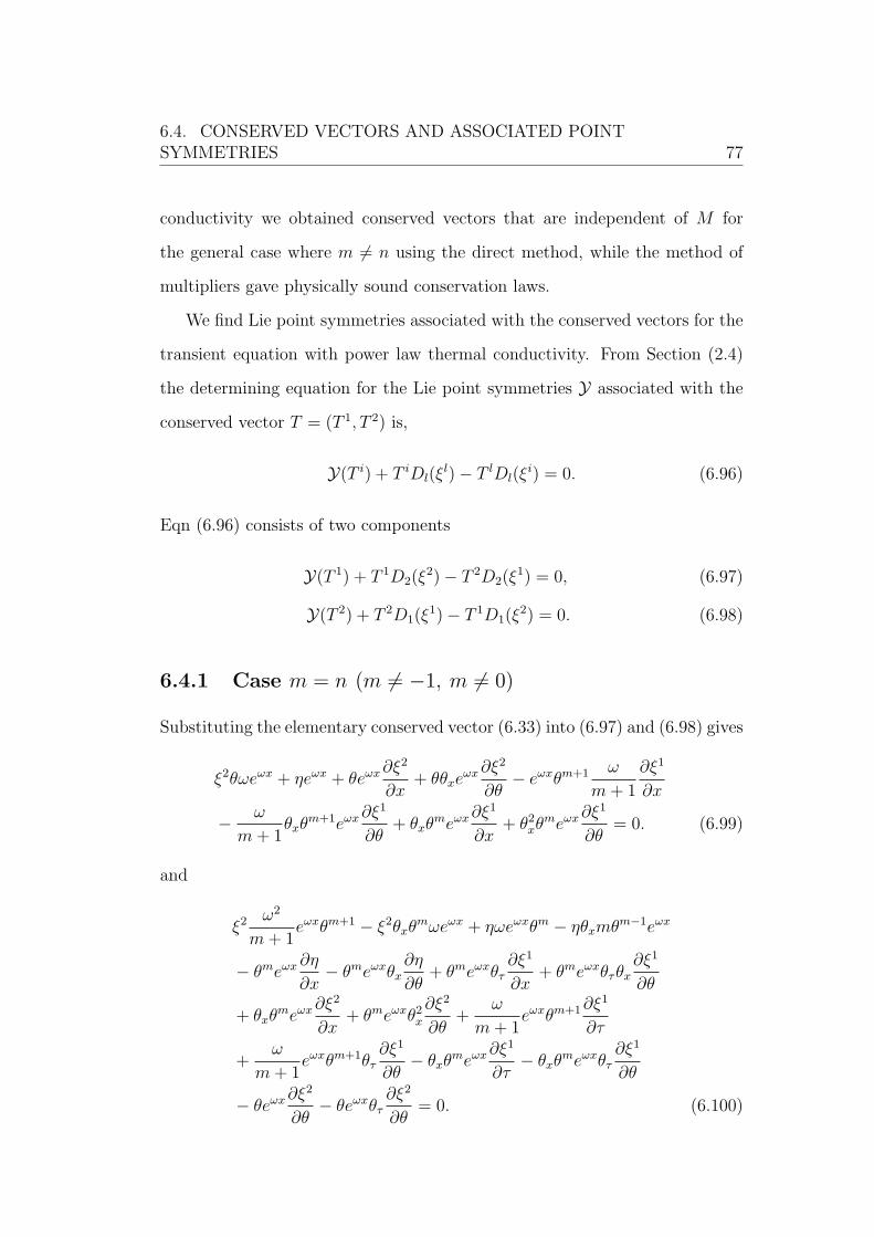
6.4. CONSERVED VECTORS AND ASSOCIATED POINTSYMMETRIES 77
conductivity we obtained conserved vectors that are independent of M for
the general case where m = n using the direct method, while the method of
multipliers gave physically sound conservation laws.
We find Lie point symmetries associated with the conserved vectors for the
transient equation with power law thermal conductivity. From Section (2.4)
the determining equation for the Lie point symmetries Y associated with the
conserved vector T = (T 1, T 2) is,
Y(T i) + T iDl(ξl)− T lDl(ξ
i) = 0. (6.96)
Eqn (6.96) consists of two components
Y(T 1) + T 1D2(ξ2)− T 2D2(ξ
1) = 0, (6.97)
Y(T 2) + T 2D1(ξ1)− T 1D1(ξ
2) = 0. (6.98)
6.4.1 Case m = n (m = −1, m = 0)
Substituting the elementary conserved vector (6.33) into (6.97) and (6.98) gives
ξ2θωeωx + ηeωx + θeωx∂ξ2
∂x+ θθxe
ωx∂ξ2
∂θ− eωxθm+1 ω
m+ 1
∂ξ1
∂x
− ω
m+ 1θxθ
m+1eωx∂ξ1
∂θ+ θxθ
meωx∂ξ1
∂x+ θ2xθ
meωx∂ξ1
∂θ= 0. (6.99)
and
ξ2ω2
m+ 1eωxθm+1 − ξ2θxθ
mωeωx + ηωeωxθm − ηθxmθm−1eωx
− θmeωx∂η
∂x− θmeωxθx
∂η
∂θ+ θmeωxθτ
∂ξ1
∂x+ θmeωxθτθx
∂ξ1
∂θ
+ θxθmeωx
∂ξ2
∂x+ θmeωxθ2x
∂ξ2
∂θ+
ω
m+ 1eωxθm+1∂ξ
1
∂τ
+ω
m+ 1eωxθm+1θτ
∂ξ1
∂θ− θxθ
meωx∂ξ1
∂τ− θxθ
meωxθτ∂ξ1
∂θ
− θeωx∂ξ2
∂θ− θeωxθτ
∂ξ2
∂θ= 0. (6.100)

6.4. CONSERVED VECTORS AND ASSOCIATED POINTSYMMETRIES 78
Separating Eqn (6.99) by derivatives of θ we find
θ2x : θmeωx∂ξ1
∂θ= 0, (6.101)
θx : θeωx∂ξ2
∂θ− ω
m+ 1θm+1eωx
∂ξ1
∂θ+ θmeωx
∂ξ1
∂x= 0, (6.102)
rem : ξ2θωeωx + ηeωx + θeωx∂ξ2
∂x− eωxθm+1 ω
m+ 1
∂ξ1
∂x= 0. (6.103)
Separating Eqn (6.100) by derivatives of θ we find
θ2x : θmeωx∂ξ2
∂θ= 0, (6.104)
θx : −ξ2θmωeωx − ηmθm−1eωx − θmeωx∂η
∂θ
+ θmeωx∂ξ2
∂x− θmeωx
∂ξ1
∂τ= 0, (6.105)
θτ : θmeωx∂ξ1
∂x+
ω
m+ 1eωxθm+1∂ξ
1
∂θ− θeωx
∂ξ2
∂θ= 0, (6.106)
rem : ξ2ω2
m+ 1eωxθm+1 + ηωeωxθm − θmeωx
∂η
∂x
+ω
m+ 1eωxθm+1∂ξ
1
∂τ− θeωx
∂ξ2
∂τ= 0. (6.107)
From Eqns (6.101), (6.102) and (6.104)
ξ1 = ξ1(τ), (6.108)
and
ξ2 = ξ2(τ, x). (6.109)
Equation (6.103) reduces to
ξ2θω + η + θ∂ξ2
∂x= 0, (6.110)
thus
η = −ξ2θω − θ∂ξ2
∂x, (6.111)
and
∂η
∂x= −ωθ
∂ξ2
∂x− θ
∂2ξ2
∂x2. (6.112)

6.4. CONSERVED VECTORS AND ASSOCIATED POINTSYMMETRIES 79
Substituting Eqns (6.111) and (6.112) into Eqn (6.107) gives
ξ2ω2
m+ 1θm+1 − ω2θm+1ξ2 − ωθm+1∂ξ
2
∂x+ ωθm+1∂ξ
2
∂x
+ θm+1∂2ξ2
∂x2+
ω
m+ 1θm+1∂ξ
1
∂τ− θ
∂ξ2
∂τ= 0. (6.113)
Separating Eqn (6.113) by powers of θ gives
θ :∂ξ2
∂τ= 0, (6.114)
θm+1 : ξ2ω2
m+ 1− ω2ξ2 +
∂2ξ2
∂x2+
ω
m+ 1
∂ξ1
∂τ= 0. (6.115)
Differentiating Eqn (6.115) with respect to τ and solving ξ1 gives
ξ1(τ) = a1τ + a2 (6.116)
where a1 and a2 are constants.
Substituting ξ1 into Eqn (6.105) and solving for ξ2 we obtain
ξ2(x) =a1mω
+ a2e−ωmx
2+m , (6.117)
where m = −2. With the explicit expressions for ξ1 and ξ2, substituting into
Eqn (6.111) gives
η = −ωθ
(a1mω
+ a2e−ωmx
2+m
)+ θ
(a2mω
e−ωmx2+m
). (6.118)
The Lie point symmetries are given by
Y1 =∂
∂τ+ e−
ωmx2+m
∂
∂x+
{(1
mω− ω
)θ exp
(− mωx
2 +m
)}∂
∂θ, (6.119)
Y2 = τ∂
∂τ+
1
mω
∂
∂x− θ
m
∂
∂θ. (6.120)
6.4.2 Case m = n (n = −1, m = −1, m = 0)
The method of multipliers gave conserved vectors that depend on the M .
Substituting the elementary conserved vector (6.52) into (6.97) and (6.98)

6.4. CONSERVED VECTORS AND ASSOCIATED POINTSYMMETRIES 80
gives
η + θ∂ξ2
∂x+ θθx
∂ξ2
∂θ+ θmθx
∂ξ1
∂x+ θmθ2x
∂ξ1
∂θ− xM2∂ξ
1
∂x− xM2∂ξ
1
∂θ= 0.
(6.121)
and
ξ2M2 −mηθxθm−1 − θm
∂η
∂x− θmθx
∂η
∂θ+ θτθ
m∂ξ1
∂x− θτθxθ
m∂ξ1
∂θ
+ θxθm∂ξ2
∂x+ θmθ2x
∂ξ2
∂θ− θmθx
∂ξ1
∂τ− θτθxθ
m∂ξ1
∂θ+ xM2∂ξ
1
∂τ
+ xM2θτ∂ξ1
∂θ− θ
∂ξ2
∂τ− θθτ
∂ξ2
∂θ= 0. (6.122)
Separating Eqn (6.121) by derivatives of θ we find
θ2x : θm∂ξ1
∂θ= 0, (6.123)
θx : θ∂ξ2
∂θ+ θm
∂ξ1
∂x− xM2∂ξ
1
∂θ= 0, (6.124)
rem : η + θ∂ξ2
∂x− xM2∂ξ
1
∂x= 0. (6.125)
Separating Eqn (6.122) by derivatives of θ we find
θ2x : θm∂ξ2
∂θ= 0, (6.126)
θx : −mηθm−1 − θm∂η
∂θ+ θm
∂ξ2
∂x− θm
∂ξ1
∂τ= 0, (6.127)
θτ : θm∂ξ1
∂x+ xM2∂ξ
1
∂θ− θ
∂ξ2
∂θ= 0, (6.128)
rem : ξ2M2 − θm∂η
∂x+ xM2∂ξ
1
∂τ− θ
∂ξ2
∂τ= 0. (6.129)
From Eqns (6.123), (6.126) and (6.124)
ξ1 = ξ1(τ), (6.130)
and
ξ2 = ξ2(τ, x). (6.131)
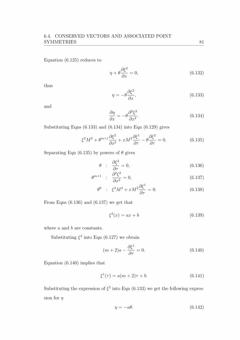
6.4. CONSERVED VECTORS AND ASSOCIATED POINTSYMMETRIES 81
Equation (6.125) reduces to
η + θ∂ξ2
∂x= 0, (6.132)
thus
η = −θ∂ξ2
∂x, (6.133)
and
∂η
∂x= −θ
∂2ξ2
∂x2. (6.134)
Substituting Eqns (6.133) and (6.134) into Eqn (6.129) gives
ξ2M2 + θm+1 ∂ξ2
∂x2+ xM2∂ξ
1
∂τ− θ
∂ξ2
∂τ= 0. (6.135)
Separating Eqn (6.135) by powers of θ gives
θ :∂ξ2
∂τ= 0, (6.136)
θm+1 :∂2ξ2
∂x2= 0, (6.137)
θ0 : ξ2M2 + xM2∂ξ1
∂τ= 0. (6.138)
From Eqns (6.136) and (6.137) we get that
ξ2(x) = ax+ b (6.139)
where a and b are constants.
Substituting ξ2 into Eqn (6.127) we obtain
(m+ 2)a− ∂ξ1
∂τ= 0. (6.140)
Equation (6.140) implies that
ξ1(τ) = a(m+ 2)τ + b. (6.141)
Substituting the expression of ξ2 into Eqn (6.133) we get the following expres-
sion for η
η = −aθ. (6.142)

6.5. CONCLUDING REMARKS 82
The Lie point symmetries are given by
Y1 = (m+ 2)τ∂
∂τ+ x
∂
∂x− θ
∂
∂θ, (6.143)
Y2 =∂
∂τ+
∂
∂x. (6.144)
6.5 Concluding remarks
The two methods considered, namely, the direct method and the method of
multipliers yielded the same results for conservation laws for transient heat
conduction through fins. Two conservation laws were derived for nonlinear
heat equation with power law thermal conductivity, one of which was the
elementary conservation law. Two cases were considered, (i) exponent of the
thermal conductivity being the same as the exponent of the heat transfer
coefficient, (ii) distinct exponents. Conserved vectors which depended on at
most first order partial derivatives were considered [56].
Higher order conservation laws could be investigated by considering con-
served vectors which depend on higher order spatial derivatives. The analysis
will be computationally laborious and may best be done with the aid of com-
puter programs. Furthermore, non trivial conservation laws may be construct-
ed if the thermal conductivity is the same as the heat transfer coefficient. This
is a very ideal/special case and may not always be true for heat transfer in
fins.

Chapter 7
Conclusions
In this dissertation, the DTM was used to construct analytical-series solutions
for nonlinear heat conduction equations for heat transfer in longitudinal fins.
The 1D DTM was used to solve the steady state ordinary differential equations.
A comparison was made between the 1D DTM series solutions of 15 terms and
the exact solutions. It is found that the solutions agreed well with the exact
solution and very small absolute errors were noted. Analytical solutions for
the boundary value problems were obtained for special cases of the exponent
n that signify the types of movement of heat through the fin.
Perhaps the notable advantage of the DTM is the generalization of the
Taylor method to problems involving unusual derivative procedures such as
fractional, fuzzy or q-derivative [54]. Some generalizations have been made by
Obidat et al. [55] and they referred to their new method as the Generalized
Differential TransformMethod (GDTM). This showed great improvement com-
pared to the Fractional Differential Transform Method (FDTM) introduced by
Arikoglu and Ozkol [57].
We note that given differential equations such as Eqns (3.11) and (3.5)
with a power law heat transfer coefficient of a fractional exponent, then one
83

84
can easily remove the fraction by basic exponential rules and employment of
the binomial expansion. However, using the DTM, one runs into difficulty
if the power law thermal conductivity in the same equation is given by the
fractional exponent. We do not know whether these observations call for the
’modified’ DTM to solve problems arising in heat flow through fins with other
profiles, such as longitudinal triangular, concave parabolic and so on, and also
with fractional power law thermal conductivity.
For the transient state problems, we employed the 2D DTM methods and
the effects of thermal parameters appearing in the equation on temperature
have been studied. Finally we sort the conservation laws and associated Lie
point symmetries. We note that the direct method and the multiplier method
gave similar results for some special cases of exponents of power laws. Mhlongo
et al.[58], have shown that exact solutions maybe constructed for these cases.

Bibliography
[1] A.D. Kraus, A. Aziz and J. Welte, Extended surface heat transfer, John
Wiley and Sons, INC, New York, 2001.
[2] D.Q. Kern, A.D. Kraus, Extended Surface Heat Transfer, McGraw-Hill,
New York, 1972.
[3] A. Moradi, Analytical solutions for fin with temperature dependent heat
transfer coefficient, Int. Journal of Engineering and Applied Sciences, 3(2):
1-12, 2011.
[4] M.H. Chowdhury and I. Hashim, On decomposition solutions of fins with
temperature dependent surface heat flux: multi-boiling heat transfer, IMT-
GT, University of Sains Malaysia, Penang, 2006.
[5] R.J. Moitsheki, T. Hayat, M.Y. Malik, Some exact solutions of the fin prob-
lem with a power law temperature-dependant thermal conductivity, Nonlin-
ear Analysis: Real World Applications, 11: 3287-3294, 2010.
[6] R.J. Moitsheki, Steady one-dimensional heat flow in a longitudinal triangu-
lar and parabolic fin, Communications in Nonlinear Science and Numerical
Simulation, 16(10): 3971-3980, 2011.
85

BIBLIOGRAPHY 86
[7] Mo. Miansari, D.D. Ganji, Me. Miansari, Application of He’s variational
iteration method to nonlinear heat transfer equations, Physics Letters A,
372(6): 779-785, 2006.
[8] C.H. Chiu, C.K. Chen, A decomposition method for solving the convective
longitudinal fins with variable thermal conductivity, International Journal
of Heat and Mass transfer, 45(10): 2067-2075, 2002.
[9] A. Rajabi, Homotopy pertubation method for fin efficiency of convective
straight fins with temperature-dependent thermal conductivity, Physics Let-
ters A, 364(1): 33-37, 2007.
[10] G. Dommairy, M. Fazeli, Homotopy analysis method to determine the fin
efficiency of convective straight fins with temperature-dependent thermal
conductivity, Communications in Nonlinear Science and Numerical Simula-
tion, 14(2): 489-499, 2009.
[11] A. Campo, R.J. Spaulding, Coupling of the methods of successive ap-
proximations and undetermined coefficients for the prediction of the ther-
mal behaviour of uniform circumferential fins, Heat and Mass Transfer, 34:
461-468, 1999.
[12] A. Campo, F. Rodriguez, Approximate analytical temperature solution
for uniform annular fins by adapting the power series method, International
Communications in Heat and Mass Transfer, 25(6): 809-818, 1998.
[13] P.L. Ndlovu and R.J. Moitsheki, Analytical solutions for steady heat
transfer in longitudinal fins with temperature dependent properties, sub-
mitted for publication, 2013.
BIBLIOGRAPHY 87
[14] R. Chiba, Application of differential transform method to thermoelastic
problem for annular disks of variable thickness with temperature-dependent
parameters, International Journal of Thermophysics, 33:363-380, 2012.
[15] S. Sadri, M.R. Raveshi, S. Amiri, Efficiency analysis of straight fin with
variable heat transfer coefficient and thermal conductivity, Journal of Me-
chanical Science and Technology, 26(4):1283-1290 (2012).
[16] A.A. Joneidi, D.D. Ganji, M. Babaelahi, Differential transform method
to determine fin efficiency of convective straight fins with temperature de-
pendant thermal conductivity, International Communications in Heat and
Mass Transfer, 36:757-762, 2009.
[17] J.K. Zhou, Differential transform method and its applications for electric
circuits, Huazhong University Press, Wuhan, China, 1986.
[18] H. Jafari, M. Alipour and H. Tajadodi, Two-dimensional differential trans-
form method for solving nonlinear partial differential equations, Internation-
al Journal of Research and Reviews in Applied Sciences, 2(1): 47-52, 2010.
[19] P.L. Ndlovu and R.J. Moitsheki, Applications of the two-dimensional
differential transform method to transient heat conduction problem
for heat transfer in longitudinal rectangular fins, Communication-
s in Nonlinear Science and Numerical Simulation, In Press, doi:
http://dx.doi.org/10.1016/j.cnsns.2013.02.019.
[20] R. Bhadauria, A.K. Singh, D.P Singh, A mathematical model to solve
reaction diffusion equation using differential transformation method, Inter-
national Journal of Mathematics Trends and Technology, 2(2):26-31, 2011.

BIBLIOGRAPHY 88
[21] M.J. Jang, C.L. Chen, Y.C. Liy, Two-dimensional differential transform
for partial differential equations, Applied Mathematics and Computation,
121:261-270, 2001.
[22] M. Merdan and A. Gokdogan, Approximate analytic solution of the heat
equation in the cast-mould heterogeneous domain by differential transfor-
mation method, J. Appl. Comp. Math., 1(3):1-4, 2012.
[23] O.O. Vaneeva, A.G. Johnpillai, R.O. Popovych and C. Sophocleous,
Group analysis of nonlinear fin equations, Applied Mathematics Letters,
21(3): 248-253, 2008.
[24] M. Pakdemirli and A. Z. Sahin, Similarity analysis of a nonlinear fin
equation, Applied Mathematics Letters, 19(4): 378-384, 2006.
[25] R.J. Moitsheki and C. Harley, Transient heat transfer in longitudinal fins
of various profiles with temperature-dependent thermal conductivity and
heat transfer coefficient, PRAMANA Journal of Physics, 77(3): 519-532,
2011.
[26] A.H. Bokhari, A.H. Kara and F.D. Zamana, A note on a symmetry anal-
ysis and exact solutions of a nonlinear fin equation, Applied Mathematics
Letters, 19(12): 1356-1360, 2006.
[27] R. Naz, F.M. Mahomed and D.P. Mason, Comparison of different ap-
proaches to conservation laws for some partial differential equations in fluid
mechanics, Applied Mathematics and Computation, 205(1): 212-230, 2008.
[28] A.H. Kara and F.M. Mahomed, Relationship between symmetries and
conservation laws, International Journal of Theoretical Physics, 39(1):
23-40, 2000.
BIBLIOGRAPHY 89
[29] G. Bluman, Connections between symmetries and conservation laws, Sym-
metry, Integrability and Geometry: Methods and Applications, 1: Pa-
per:011, 2005.
[30] S.C. Anco and G.W. Bluman, Direct construction method for conservation
laws of partial differential equations. Part I: Examples of conservation clas-
sifications, European Journal of Applied Mathematics, 13: 545-566, 2002.
[31] M. Ghafoori, M. Motevalli, M.G. Nejad, F. Shakeri, D.D. Ganji, M. Jalaal,
Efficiency of differential transformation method for nonlinear oscillation:
comparison with HPM and VIM, Current Applied Physics, 11(4): 965-971,
2011.
[32] P.J. Olver, Applications of Lie groups to differential equations, Springer-
Verlag, New York, 1993.
[33] G.W. Bluman ans S.C. Anco, Symmetry and integration methods for
differential equations, Springer-Verlag, New York, 2002.
[34] G.W. Bluman, A.F. Cheviakov and S.C. Anco, Applications of symmetry
methods to partial differential equations, Springer-Verlag, New York, 2010.
[35] H. Stephani, Differential equations: Their solutions using symmetries,
Cambridge University Press, 1989.
[36] J.M. Hill, Differential equations and group methods for scientists and
engineers, CRC Press, Boca Raton, 1992.
[37] N.H. Ibragimov, Elementary Lie group analysis and ordinary differential
equations, John Wiley and Sons, New York, 1999.
[38] A.T.S. Wan, Finding conservation laws for partial differential equations,
M.Sci. Thesis, The University of British Columbia, 2010.
BIBLIOGRAPHY 90
[39] P.D. Lax, Hyperbolic Systems of Conservation Laws and the Mathemat-
ical Theory of Shock Waves, CBMS-NSF Regional Conference in Applied
Math., SIAM, 1973.
[40] A.H. Kara and F.M. Mahomed, A basis of conservation laws for par-
tial differential equations, Journal of Nonlinear Mathematical Physics, 9(2):
60-72, 2002.
[41] P.S. Laplace, (English translation, Celestial Mechanics, New York, 1966),
1798.
[42] H.C. Unal, An analytical study of boiling heat transfer from a fin, Inter-
national Journal of Heat Mass Transfer, 30(2): 341-349, 1987.
[43] A. Aziz, T.Y. Na, Periodic Heat Transfer in Fins with Variable Thermal
Conductivity, Int. J. Heat Transfer, 24(8):1397-1404, 1981.
[44] A. Moradi, H. Ahmadikia, Analytical solution for different profiles of fin
with temperature-dependent thermal conductivity, Mathematical Problems
in Engineering, 2010: Article ID: 568263, 2010.
[45] R.J. Moitsheki, Steady heat transfer through a radial fin with rectangular
and hyperbolic profiles, Nonlinear Analysis: Real World Applications, 12(2):
867-874, 2011.
[46] S. Vitanov, V. Palankovski, S. Maroldt and R. Quay, High temperature
modeling of AlGaN/GaV HEMTs, Solid State Electron 54(10):1105-1112,
2010.
[47] A. Jezowski,B.A. Danilchenko, M. Boekowski, I. Grzegory, S. Krukowski,
T. Suski and T. Paszkiewicz, Thermal conductivity of GaN crystals in 4.2-
300k range, Solid State Communications, 128: 69-73, 2003.

BIBLIOGRAPHY 91
[48] A.F. Mills, Basic heat and mass transfer: Second Edition, Prentice Hall,
1999.
[49] M.-H. Chang, A decomposition solution for fins with temperature depen-
dent surface heat flux, International Journal of Heat and Mass Transfer,
48(9): 1819-1824, 2005.
[50] D.D.Ganji, M.Rahgoshay, M.Rahimi and M.Jafari, Numerical investiga-
tion of fin efficiency and temperature distribution of conductive, convective
and radiative straight fins, International Journal of Research and Reviews
in Applied Sciences, 4:3, Special Issue:1, 2010.
[51] A. Aziz and M. Torabi, Convective-radiative fins with simultaneous varia-
tion of thermal conductivity, heat transfer coefficient, and surface emissivity
with temperature, Heat Transfer - Asian Research, 41(2): 99-113, 2012.
[52] E. Noether, Invariant variation problems, Transport Theory and Statisti-
cal Physics, 1(3):183-207 (1971).
[53] M. Anthonyrajah, D.P. Mason, Conservation laws and invariant solutions
in the Fanno model in turbulent compressible flow, Mathematical and Com-
putational Applications, 15(4): 529-542, 2010.
[54] C. Bervillier, Status of the differential transform method, Applied Math-
ematics and Computation, 218: 10158-10170, 2012.
[55] Z. Obidat, S. Momani, V.S. Erturk, Generalized Differential Transform
Method: application to differential equations of fractional order, Applied
Mathematics and Computation, 197(2): 467-477, 2008.

BIBLIOGRAPHY 92
[56] P.L. Ndlovu and R.J. Moitsheki, Conservation laws and associated Lie
point symmetries admitted by the transient heat conduction problem for
heat transfer in straight fins, submitted for publication, 2013.
[57] A. Arikoglu, I. Ozkol, Solution of fractional differential equations by
using the differential transform method, Chaos, Solitons and Fractals 34:
1473-1481, 2007.
[58] M.D. Mhlongo, R.J. Moitsheki and O.D. Makinde, Transient response of
longitudinal rectangular fins to step change in base temperature and in base
heat flow conditions, International Journal of Heat and Mass Transfer, 57:
117-125, 2013.
Recommended