Analysis of Ethernet-like protocols
Andrey Lukyanenko
University of Kuopio
History of Ethernet
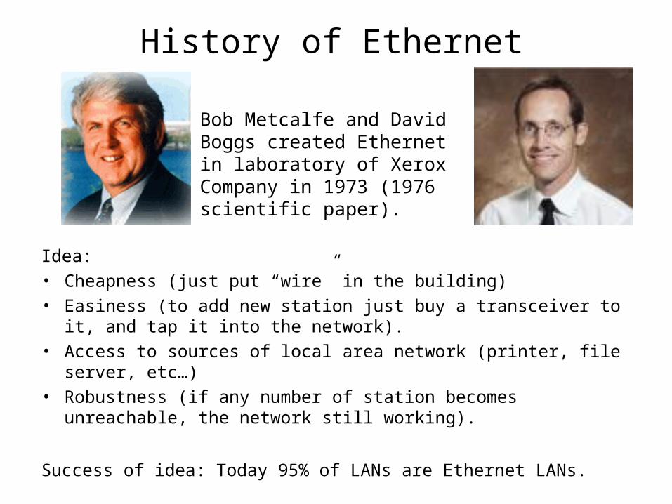
Bob Metcalfe and David Boggs created Ethernet in laboratory of Xerox Company in 1973 (1976 scientific paper).
Idea:• Cheapness (just put “wire” in the building)• Easiness (to add new station just buy a transceiver to it, and tap it
into the network).• Access to sources of local area network (printer, file server, etc…)• Robustness (if any number of station becomes unreachable, the
network still working).
Success of idea: Today 95% of LANs are Ethernet LANs.

The Idea
• Shared medium (bus).– all data simply broadcast over the
medium.
– receivers listen to the network, if there is a message for them.
• Collisions.– If two or more messages broadcast in
the network then collision could happen.
• Backoff protocol from Aloha.– The part of collision resolution protocol.
– Problem of algorithms with fixed retransmission time (Pure Aloha isn’t stable).

Collision resolutionMechanisms to reduce probability and cost of losing packets:1. Carrier detection
• Phase encoded (to remove silent spaces during packet transfer)• If a station wants to transfer a packet it listen to the channel, deferring the packet if
the channel busy.• Collisions only if two or more stations find the Ether silent.
2. Interference detection • each transceiver has detector, which says if the channel has the same signal that it
transmits. If the signal differ then collision.• We define time slot from now as double time to propagate the signal over network
(round trip time).
3. Packet error detection (checksums)4. Truncated packet filtering (reduce processing load).5. Collision consensus enforcement
• When station find it message experenced interference it jams the network, to let all station know about it.

Backoff protocol in Ethernet
• Metcalfe and Boggs took binary exponential backoff protocol for their network.
• Difference that isn’t anymore a constant, now it is a function from the number of successive collisions of a message (backoff counter ).
• In Ethernet this function have the following form .
• If backoff counter exceeds 16, then we discard the message and zero the counter.
• Time delay always is a random number that is taken uniformly from sector We work with time delay before next attempt to send instead of “clear” probability .
f
ib
)10,min(2 ibf
)2,1( )10,min( ib
f

Why do we continue study the Ethernet?
Answer: We can use backoff protocol in the future.
Examples of use:
1. Wireless network (also took binary exponential backoff).
2. OCPC (optical comunication parallel computer)
• h-relation problem currently studied in Kuopio.
• Collisions happen when two or more station transmit to the same station at some moment of time.
• Every station has h messages to send.
• The expected number of messages to some
station is h (some kind of balanced situation).

h-relation problem (closer view)
Tasks:• In h-relation problem backoff protocol may be used.• We need to choose the best one. • In general we can take any kind of backoff function, backoff protocol
wasn’t studied quite well yet (though, but some results say that binary exponential isn’t good choice).

History of researchDifferent authors got different results on backoff. • Kelly
– mathematically formulation of problem (binary), criterion of instability with high input rate, for infinite model.
• Aldous – Ultimate instability of all acknowledge-based protocols, for infinite
model.• Goodman et al
– stability for small incoming rate, for finite model.• Håstad et al
– Instability of binary exponential backoff for big incoming rate (>0.5)– Stability of polynomial backoff.– Instability of linear and sublinear protocols at all.
• Shenker– Denies some results of Håstad et al (according polynomial backoff)

Main Results by now
• For infinite model (when number of station is infinite) the protocol is unstable for all backoffs.
• For finite model polynomial backoff stable, and binary exponential unstable for big incoming rate (>0.5) and stable for small incoming rate, which goes to zero as the number of station grows up.

Our model
• Model was taken from Kwak et al paper.• It’s slightly differ from model in Bianchi.
• Assumptions of the model:– The model is under Saturation conditions.– The model is in steady state (collision probability is the same,
this state we could achieve if let the model work for a long period of time).
– Time slotted model (with slot equal to the double round trip time). Message broadcasts during one time slot and has exactly bounds of the slot (also synchronized).

Calculus (1)
Our first task for this model was to find the dependence
between probability to transmit and probability to collide at
any moment of time. We found that
where
From Bianchi we have that
so solution of this system gives us the exact value for
probability of collision (unfortunately we couldn’t solve it in
general).
Note that function F(z) has all the properties of backoff functions
(combined together).

Calculus (2)
Solving the previous equations we
have, that
The condition to have exactly
one intersection is
0 0.2 0.4 0.6 0.8 10
200
400
500
0
Qf x( )
Lf x( )
Ef x( )
Subf x( )
L x( )
10 x

Calculus (3)
One of the most important characteristic of a network is the delay time
of the system. It’s time that message should wait until successful
transmission:
Combining it with we can find the
value of optimal probability of collision

Calculus (4)
• Existing BEB:
• Optimal EB:
0.34
0.36
0.38
0.4
0.42
0.44
0.46
0.48
0.5
10 20 30 40 50 60 70 80 90 100
f(x)
0.36
0.37
0.38
0.39
0.4
0.41
0.42
0.43
0.44
0.45
0.46
0.47
10 20 30 40 50 60 70 80 90 100
f(x)

Optimality for general function

Leaving saturation condition
Using negative drift we can leave
saturation conditions.
New model is almost the same. New
node which doesn’t affect if number of
messages in the queue greater than
zero.
i = 0 i = 1 i = 2 i = 3cp
1 - pc
cp cp cp
1 - pc 1 - pc
1 - pc
1 - pc
1i =-1

Negative drift (idea).
))(|)()1(( CtQtQtQExp
Zero state
Current state
Negative drift
Q(t) > C
Q(t) < C
The number of steps to return to zero is at most (with positive probability) NtQ
)(
Condition of drift
level)-C from zero return to(P

Repeat results.
• We found optimality conditions for backoff protocol (model with infinite backoff counter).
• Extended the development of backoff to general functionality.
• Showed the performance of known backoff functions.

Future work.
• Make simulation (checking received results).
• Extend the theory on backoff function with finite model backoff counter.
• Check the formulas for small network preload (weakness of the assumption that model in steady state).

Thanks.
Questions?
Recommended