An Outlier in Zipf’s World? A Case Studyof China’s City Size and Urban Growth
The Harvard community has made thisarticle openly available. Please share howthis access benefits you. Your story matters
Citation Yin, Cathy. 2020. An Outlier in Zipf’s World? A Case Study of China’sCity Size and Urban Growth. Bachelor's thesis, Harvard College.
Citable link https://nrs.harvard.edu/URN-3:HUL.INSTREPOS:37364744
Terms of Use This article was downloaded from Harvard University’s DASHrepository, and is made available under the terms and conditionsapplicable to Other Posted Material, as set forth at http://nrs.harvard.edu/urn-3:HUL.InstRepos:dash.current.terms-of-use#LAA

An Outlier in Zipf’s World?
A Case Study of China’s City Size and Urban Growth
Lei (Cathy) Yin
Presented to the Department of Applied Mathematics
in partial fulfillment of the requirements
for a Bachelor of Arts degree with Honors
Harvard College
Cambridge, Massachusetts
April 3, 2020

i
Abstract
This paper examines the population distribution and urban growth patterns of Chinese cities,
motivated by two stylized facts – Zipf’s law and Gibrat’s law for cities. Our findings suggest that
China deviates from both laws from 1991 to 2017. In particular, its population is distributed more
equally than Zipf’s law would otherwise predict, and Chinese cities have experienced a significant
mean reversion, rather than a homogenous growth path.
We develop three hypotheses for explaining why large cities experience slower urban growth in
China, namely, economic productivity slowdown, amenity deterioration, and direct government
interventions. Our results indicate that in China, productivity and amenities promote population
growth, and large cities enjoy higher productivity and better amenities. On the other hand, China’s
population control policies, the one-child policy and the household registration (hukou) system,
are more strictly enforced in large cities than in small and medium-size cities. Therefore, large
cities grow slower due to direct government interventions, despite their higher productivity and
better amenities.

ii
Executive Summary
Zipf’s law is a well-known empirical rule which fits the city size distribution for countries across
the world well generally, but we find that China seems to deviate substantially from it in the past
three decades. In particular, the population is distributed more equally in China than Zipf’s law
would otherwise predict, and there are far fewer megacities despite its huge population. To explain
this departure from the norm, we examine whether Gibrat’s law, the underlying assumption of
Gabaix’s (1999) Zipf’s law model, holds in China. Instead of the homogenous growth path
suggested by Gibrat’s law, we observe a significant mean reversion of city sizes from 1991 to 2017.
This pattern of mean reversion grows weaker over time. Our paper then develops three main
hypotheses for explaining why large cities experience slower urban growth in China, namely,
economic productivity slowdown, amenity deterioration, and direct government interventions. We
exploit city-level urban characteristics data and conduct analyses to test these three hypotheses.
We use a linear regression model for studying how economic productivity and urban amenities
connect to urban growth and population size. We find that although these two factors indeed
promote population growth as suggested by spatial equilibrium models, large cities in China enjoy
both higher productivity and better amenities. Thus, the two urban growth determinants that apply
to most countries cannot explain China’s growth convergence. As for our third hypothesis, we
investigate whether the city-level enforcement intensity of China’s two main population control
policies, the one-child policy and the household registration (hukou) system, increases in
population size. We implement a differences-in-differences approach to quantify the effects of the
nationwide relaxation of the universal one-child policy in 2011 on the rate of natural increase (RNI)
for cities. Empirical evidence shows that relative to small cities, large cities suffered from lower
RNI under the universal one-child policy and experienced a rise in RNI after the policy relaxation.
We run a simple linear regression using the ratio of unofficial migrants to hukou population as a
proxy for the strictness of the hukou system and find that such ratio decreases in population size.
Our results indicate that China’s population control policies are more constraining for large cities
than for small and medium-size cities. Therefore, even though large cities are more appealing in
terms of higher productivity and better amenities, populations grow slower because the
government wants so. One implication for Zipf’s law is that as China continues to loosen its birth
planning and migration control in the 2010s, future convergence to Zipf’s law may be plausible.

iii
Acknowledgments
First and foremost, I would like to express my sincere gratitude to my supervisor Professor
Kenneth Rogoff. Thank you for guiding me and supporting me throughout my research and thesis
writing process. I would not be able to complete this thesis without your patience, encouragement,
enthusiasm, and immense knowledge. Your advice on economic research is truly invaluable for
all my future endeavors.
I would like to thank Professor Edward Glaeser for critiquing my work and providing me with
crucial advice on the methodology for studying urban growth. I would also like to thank Professor
Gabaix Xavier for discussing his works on the topic of Zipf’s law with me.
I would like to thank my thesis seminar instructor, Dr. Judd Cramer, for keeping me on track. I
greatly appreciate your constant feedback and innovative solutions to all the problems I faced
along the way. I would also like to thank Dr. Gregory Bruich for his help with econometrics.
Last, but not least, thank you to my family and friends for your continuous encouragement and
support throughout my college journey. I am beyond grateful that you have all helped shape me
into the person I am today, pushed me to reflect on every single piece of my experiences, and stood
by me even in the hardest of times.

iv
Contents
1 Introduction ............................................................................................................................. 1
2 Background ............................................................................................................................. 5
2.1 Relevant Literature.......................................................................................................... 5
2.2 Overview of China’s Urban Development and Policies ................................................. 7
3 Conceptual Framework ......................................................................................................... 10
3.1 Zipf’s Law Model ......................................................................................................... 10
3.2 Gibrat’s Law Model ...................................................................................................... 13
3.3 Spatial Equilibrium Model ............................................................................................ 14
4 Data ....................................................................................................................................... 18
4.1 Urban Population Data .................................................................................................. 18
4.2 Urban Characteristics Data ........................................................................................... 24
5 Methodology ......................................................................................................................... 27
6 Results ................................................................................................................................... 38
6.1 Repeated Cross-Sectional OLS Regression for Zipf Coefficients ................................ 38
6.2 Correlation between Urban Population Growth and Initial Urban Size ....................... 44
6.3 City Growth Regressions .............................................................................................. 49
6.4 Public Sector Rule Regressions .................................................................................... 65
7 Discussion ............................................................................................................................. 71
8 Appendix ............................................................................................................................... 75
9 Reference .............................................................................................................................. 81

1
1 Introduction
Zipf’s law strikes urban economists with its simplicity and empirical validity in capturing
the distribution of city sizes. Most countries are believed to obey Zipf’s law quite well, but the
majority of studies on China suggest a deviation from it (Song and Zhang, 2002; Anderson and
Ge, 2005; Luckstead and Devados, 2014). Some argue this exception is attributable to a violation
of the homogenous growth process, or Gibrat’s law, by Chinese cities (Chauvin et al., 2017).
Others believe China’s unique urbanization and public policies may explain its departure from
Zipf’s law, albeit with little empirical evidence (Song and Zhang, 2002). Our paper contributes to
the debate by examining economic and policy factors that may cast light on why China’s city size
distribution deviates from Zipf’s law, and in particular, why the large cities do not grow as large
as Zipf’s law predicts. We ultimately find that the stricter enforcement of government’s population
control policies in large cities, rather than the productivity slowdown or rising urban issues, is
responsible for the slower population growth of large cities in China.
Zipf’s law says that graphing the logarithm of city ranks in terms of population size against
the logarithm of city populations, we obtain a straight line with -1 as the slope coefficient. Figure
1 below presents a visualization of Zipf’s law taken from Arshad et al. (2018) using data of the
largest 135 U.S. metropolitan areas in the census year 2010. The slope of the fitted line is −1.019.
In terms of distribution, Zipf’s law states that the probability of a city size being greater than some
threshold S is proportional to 1/S. This is a special case of the well-known Pareto distribution
Prob(size > S) = aS−ζ, with the Pareto coefficient equal to one (ζ = 1).

2
Figure 1. Log Size versus Log Rank of the Largest 135 U. S. Metropolitan Areas in 2010.
Source: Statistical Abstract of the United States (2010).
Empirical testing of Zipf’s law has been conducted for different countries over different
periods and suggests that China may be an exception to Zipf’s law. The majority of studies on the
United States agree that the upper tail of city size distribution conforms to Zipf’s law (Krugman,
1996; Ioannides and Overman, 2003; Levy, 2009; Ioannides and Skouras, 2013). Other Western
matured economies, like Germany (Giesen and Südekum, 2011) and Russia (Rastvortseva and
Manaeva, 2019), have been shown to obey Zipf’s law quite well. Some developing countries, like
India (Luckstead and Devados, 2014) and Brazil (Moura and Ribeiro, 2013; Matlaba et al., 2013),
also converge to Zipf’s law after significant urbanization in recent decades. In contrast, findings
on China’s adherence have been mixed at best, and most studies suggest a rejection of Zipf’s law
(for example, Song and Zhang, 2002; Anderson and Ge, 2005; Luckstead and Devados, 2014).1
1 See Section 2.1 for a detailed summary of previous studies on China.

3
Currently the most populous country in the world, China has long been treating the
population and its distribution as a crucial “issue” to be dealt with. Various policies, including the
family planning program and the household registration system, have been enforced by the central
government since the founding of the People’s Republic of China (PRC) in 1949. Over the past
four decades, China has undergone rapid urbanization, but its city size distribution has yet to
conform to Zipf’s law. Compared with other well-studied countries that adhere to Zipf’s law,
China is unique for the central planning component in its economic and administrative policies.
To obtain a deeper understanding of how China’s policies may affect urban growth and
population distribution, we apply some well-established urban economics models to investigate
China’s case. Gabaix (1999) provides a baseline model for explaining why cities follow Zipf’s law
using a random walk with a lower barrier. One important assumption of his model is the
homogeneity of growth processes, or Gibrat’s law. That is, city growths have the same mean and
the same variance, independent of their initial sizes. Gabaix argues that deviations from Zipf’s law
can be explained by deviations from Gibrat’s law. Given China’s well-recognized deviation from
Zipf’s law, we examine whether a deviation from Gibrat’s law can also be observed and if so, what
economic or policy factors may have facilitated or hindered the convergence of city growth. To
propose potential economic factors, we consult Glaeser and Gottlieb’s (2009) generalized Rosen-
Roback spatial equilibrium framework, which shows that high productivity and high amenities are
the two underlying factors of urban population growth. As for policy factors, we focus on China’s
unique population control policies, the one-child policy and the hukou system. We then design
strategies to test whether these three hypotheses – namely, economic productivity, amenities, and
government’s population control policies - can explain China’s urban growth patterns.

4
Our results suggest that China deviates from Zipf’s law and Gibrat’s law from 1991 to
2017. In particular, large cities in China have smaller population sizes than what Zipf’s law would
grant and grow slower than small and medium-size cities. Among the three hypotheses we propose,
differences in economic productivity and amenities fail to justify why large cities have experienced
slower growth. Instead, we find that the government’s direct interventions through two population
control policies have been effective in constraining population expansion in large cities, which
explains why they grow slower and are not as large as Zipf’s law prediction. In addition, our result
(from incorporating new population data) shows that deviations from Zipf’s law and Gibrat’s law
become weaker in 2011-2017 than previous decades and is in line with China’s recent relaxation
of its population control policies.
The rest of the paper is structured as follows: Section 2 summarizes previous empirical
studies on China and reviews China’s urbanization. Section 3 presents theoretical frameworks for
Zipf’s law, Gibrat’s law, and urban growth. Sections 4 and 5 provide some background on the data
and methodology utilized in this paper to test Zipf’s law and Gibrat’s law and to explain the
population growth of Chinese cities. Empirical results are presented in Section 6. Section 7
discusses the findings in light of China’s economic and administrative policies.

5
2 Background
2.1 Relevant Literature
Previous empirical studies on whether Chinese cities obey Zipf’s law produce mixed
results using population data prior to 2010. Some show evidence of Chinese city sizes converging
to Pareto’s distribution and Zipf’s law, whereas others disagree. For example, Gangopadhyay and
Basu (2009) find that the largest Chinese cities follow a Pareto distribution with coefficient one
using data from 1990 and 2000. In contrast, Song and Zhang (2002) use city-level data from 1991
and 1998 and argue that although a Pareto distribution fits Chinese cities well, Zipf’s law is
rejected with the Pareto coefficient being statistically greater than one; Luckstead and Devadoss
(2014) obtain similar results using data from 2010. These disagreements might be attributable to
the fact that the Pareto coefficient is highly sensitive to the choice of sample size. In particular,
Peng (2010) observes that China’s Pareto coefficient is monotonically decreasing when lower
truncating points are chosen. In addition, Zipf’s law results seem to depend on the choice of city
definition. While most studies of China use the administrative definition, which corresponds to the
official reporting units, Dingel et al. (2019) argue that the night-lights-based metropolitan areas
they construct conform well to Zipf’s law using census data from 2000 and 2010. Anderson and
Ge (2005) and Li et al. (2016), on the other hand, favored a lognormal distribution over the Pareto
distribution for Chinese cities. All relevant studies on Chinese city size distribution use data prior
to 2010 for testing Zipf’s law and Pareto distribution, and our paper extends the time period of
study with new data from 2011 to 2017.
A few studies examine the underlying assumption of Zipf’s law - whether Chinese city
growth is size-independent (Gibrat’s law) - in an attempt to explain China’s deviation from Zipf’s
law; however, they do not provide insights on what factors may have caused Chinese city growth

6
to be size-dependent. Gabaix (1999) identifies the homogeneity of city growths as an important
assumption for explaining why Zipf’s law holds and recognizes that any violation of it may lead
to deviations from Zipf’s law. Evidence is again mixed for whether China’s city growth follows
Gibrat’s law. Cen (2015) and Li et al. (2016) find that Gibrat’s law approximately holds for all
Chinese cities from the 1980s to 2000s. On the contrary, Fang et al. (2017) and Chauvin et al.
(2017) observe that Chinese city growth is size-convergent before 2000 and size-independent after
2000. Gangopadhyay and Basu (2012) argue that Chinese cities experience parallel growth where
small and medium-size cities have grown faster than large cities. Likewise, cities with similar
policy regimes and natural resource endowments grow parallel in the long run (Chen et al., 2013;
Wu and He, 2017).
To explain China’s deviation from Zipf’s law and Gibrat’s law, the existing literature
identifies the role of China’s unique administrative and economic policies, but rarely supports
these hypotheses with empirical evidence. Song and Zhang (2002) and Xu and Zhu (2009) propose
several economic and institutional factors of the Chinese urban system, including rural-urban
migration restrictions imposed by the household registration system (“hukou”), China’s open-door
policy and its subsequent boosts in foreign direct investments (FDI), and government’s
development strategies that favor small and medium-size cities. In addition to the hukou system
and the economic reforms, some scholars emphasize China’s family planning program, based on
the one-child policy, in explaining China’s deviation from Zipf’s law (Anderson and Ge, 2005;
Luckstead and Devadoss, 2014). Yet, past literature discusses these policy factors qualitatively
without empirical evidence, and our paper fills this gap by collecting urban characteristics data at
the city level and designing research strategies to test the effect of each factor.

7
2.2 Overview of China’s Urban Development and Policies
As a socialist economy, the People’s Republic of China has a complex urban system and a
unique path of development since its founding in 1949. China experienced rapid population growth
from 1949 to 1958, during which the average growth rate of the non-agriculture population was
over 10 percent, with the majority of growth happened in large cities (NSB, 2000). The number of
cities also doubled within nine years. Following the initial growth was a period of stagnation from
1958 to 1978 due to the Great Leap Forward and the Cultural Revolution. During these two
decades of political turmoil, the rural population was forced to stay in their birthplace under the
collectivization of agriculture. Urban expansion thus slowed down with little growth in urban
population size and the number of cities. The year 1978 marked a turning point of urban
development when the central government introduced a series of economic reforms that attempted
to liberalize the economy. Policies involved the de-collectivization of agriculture, the opening up
to foreign investments, and the permission for entrepreneurship. As a result, China experienced
rapid urban growth in the past four decades following 1978. The non-agricultural population in
urban areas increased 126 percent from 172 million in 1978 to 389 million in 1999; the number of
officially designated cities increased from 191 to 667, and the urban share of total population
increased from 18 to 31 percent (NSB, 2000). In the last two decades, China continued its
economic reforms albeit with slower urban population growth. Large-scale privatization of
previously state-owned enterprises occurred in the late 1990s and early 2000s, leading to an
increase in total factor productivity and gross regional output levels. Meanwhile, the Chinese
government further brought down trade barriers and reduced tariffs. Such efforts peaked as China
joined the World Trade Organization (WTO) in 2001. As a result, China enjoyed a significant
increase in foreign direct investment inflows, especially to large cities, in the following years.

8
Despite the economic growth that took place in the cities, population growth dropped with the
emergence of many urban issues including crowding, congestion, pollution, and crime.
The most distinct feature of China’s urban development is its direct government
interventions. Chinese governments, from central to local levels, are far more active in planning
and containing city populations than any other country in the world. The two main policy tools
they have been using are the household registration (or “hukou”) system and the one-child policy.
In 1951, the Ministry of Public Security issued the first regulation regarding migration and
formally initiated the household registration system. By 1958, all rural and urban citizens had been
registered with the state, and rigorous control over any transfer of the hukou status had been put
into place. Since the reform and opening up in 1978, the state has loosened its restrictions on
migration from rural areas to small cities but imposed greater limits on migration into big cities
like Beijing and Shanghai. The hukou status specifies the location of residence and is, essentially,
an official permit that allows a person to stay in the designated location. Hukou also divides people
into agricultural and non-agricultural categories, where a non-agriculture hukou status grants
superior welfare benefits. In addition to issuing permits, the government implements
complementary policies that discriminate against unofficial migrants (those without permits) in
areas of job allocation, housing, education, healthcare, and social security in the city (Song, 2014).
Thus, although unofficial migrants can physically stay in the city, it is much harder for them to
live their own lives.
The one-child policy is a birth planning program of one child per family, first introduced
in 1982, to control the rapid growth of the Chinese population. Intended to be applied universally,
the one-child policy was, however, not uniformly followed across the country. It is commonly
believed that urban cities oversaw stricter enforcement with penalties on families with

9
“unauthorized” children, whereas rural families managed to find loopholes and conceive a second
child if their first one was a girl. In urban cities, 91 percent of the mothers had only one child; in
sharp contrast, only 59 percent of rural mothers followed the one-child policy (Li, 1995). Starting
from 2011, the one-child policy was somewhat relaxed across the country as China issued a new
law allowing parents who are both the only child to have a second child; it was formally replaced
by the current universal two-child policy in 2016. However, birth rates in urban areas did not
rebound significantly due to the long-lasting impact the one-child policy had created, including
the imbalanced sex-ratio and the low fertility rate.
10
3 Conceptual Framework
3.1 Zipf’s Law Model
The history of Zipf’s law dates back to Auerbach (1913) and Singer (1936), who first apply
the Pareto law to city size distribution. A mathematical statement of the Pareto law for city size
distribution is as follows
𝑟𝑖 = 𝐴 ⋅ 𝑆𝑖−𝛼 (1)
where 𝑟𝑖 is the number of cities with population 𝑆𝑖 or more, or equivalently, the rank of city i when
cities are ranked from 1 to n by their population size in descending order; 𝑆𝑖 is the population of
the city i, 𝛼 is the Pareto coefficient, and A is a constant. Equation 1 implies a linear relationship
between the logarithm of city rank and the logarithm of city size
𝑙𝑜𝑔(𝑟𝑖) = 𝑙𝑜𝑔(𝐴) − 𝛼 ⋅ 𝑙𝑜𝑔(𝑆𝑖) (2)
Zipf’s law for cities (also referred to as “the rank-size rule”) is a special case of the Pareto
law with the Pareto coefficient 𝛼 = 1 (Zipf, 1949). It states that the rank of a city is inversely
proportional to its size.
𝑟𝑖 =𝐴
𝑆𝑖 (3)
This implies that within a geographical region of cities, the largest city is about twice the size of
the second-largest city, about three times the size of the third-largest city, and so on. The Zipf-
form of Equation 1 is as follows
𝑆(𝑘) = 𝑆(1) ⋅ 𝑘−𝑞 (4)

11
where 𝑞 is equal to 1 under the special case, and 𝑆(𝑘) is the size of the kth largest city. A simple
mathematical derivation can show that 𝑞 =1
𝛼 and 𝑆(1) = 𝐴
1
𝛼. Zipf’s law holds when 𝛼 = 1 and
𝑞 = 1. If 𝛼 → ∞, then 𝑞 → 0, and 𝑆(𝑘) = 𝑆(1), ∀𝑘, suggesting a perfectly even distribution of
population as all cities have the same size.
Gabaix (1999) provides a theoretical framework for studying why some countries converge
to Zipf’s law whereas others fail to. He shows that if different cities in a region have homogenous
random growth processes, then their limit distribution will converge to Zipf’s law. Let 𝑆𝑖,𝑡 denote
the size of city i normalized by the total urban population at time t. City size follows Zipf’s law if
the upper tail distribution of city sizes at time t, 𝐺𝑡(𝑆) ≔ 𝑃(𝑆𝑡 > 𝑆), converges to some steady-
state distribution function 𝐺(𝑆) = 𝑎 ⋅ 𝑆−𝜁, where a is a constant and ζ = 1. Gabaix proves that this
statement is true if we assume all cities grow randomly with the same expected growth rate and
the same variance (Gibrat’s law). In other words, city growth rates are identically distributed and
independent of city sizes.
Gabaix further examines the case where cities grow randomly with expected growth rates
and variances dependent upon city sizes. The size of city i at time t follows the process (according
to Equation 11 ibid., p. 756)
𝑑𝑆𝑡
𝑆𝑡= 𝜇(𝑆)𝑑𝑡 + 𝜎(𝑆)𝑑𝐵𝑡 (5)
where 𝜇(𝑆) is the expected growth rate of the normalized city size 𝑆, 𝜎(𝑆) is its standard deviation,
and 𝐵𝑡 is a reflected geometric Brownian motion. It follows that the limit distribution of city sizes
will converge to Pareto’s law with the following local Zipf coefficient (also, Pareto coefficient)
𝜁(𝑆) = −𝑆
𝑝(𝑆)⋅
𝑑𝑝(𝑆)
𝑑𝑆 (6)

12
where 𝑝(𝑆) is the probability distribution of S. Then integrating the forward Kolmogorov equation
(Equation 12 ibid., p. 757) into Equation 6, Gabaix derives the general form of Zipf coefficient,
ζ(S), as a function of the mean and variance of city growth rates (according to Equation 13 ibid.,
p. 757)
𝜁(𝑆) = 1 − 2 ⋅𝜇(𝑆)
𝜎2(𝑆)+
𝑆
𝜎2(𝑆)⋅
𝜕𝜎2(𝑆)
𝜕𝑆 (7)
This general expression for the Zipf coefficient lays the foundations of our empirical approach to
explain China’s deviation from Zipf’s law. As derived in Equation 7, deviations from Zipf’s law
(ζ(S) ≠ 1) can be explained either by deviations of the expected growth rates for a range of cities
from the overall mean for all city sizes (μ(S) = γ(𝑆) − γ̅ ≠ 0) or by the dependency of the
variance of growth rates on city sizes (∂σ2(S)
∂S≠ 0). When large cities exhibit lower growth rates
(𝛾(𝑆) − �̅� < 0), their size distribution will decay faster than Zipf’s law would predict and their
local Zipf coefficient will be greater than one (ζ(S) > 1). If Gibrat’s law holds precisely, then the
second and the third term in Equation 7 equal to zero, and the Zipf coefficient ζ(S) = 1 regardless
of city size S.

13
3.2 Gibrat’s Law Model
Gibrat’s law, also known as the law of proportional growth, is first proposed by Gibrat
(1931) as an empirical regularity governing the dynamics of firm sizes and later applied to the field
of urban economics to capture city growth processes and explain the resulting population
distribution. Proportional growth states that the expected increment to a city’s size in each period
is proportional to its initial size. Let S𝑖,𝑡 be the population size of city i at time t and δt be the
proportional growth rate between period 𝑡 − 1 and 𝑡. The mathematical expression of proportional
growth is S𝑖,𝑡 − S𝑖,𝑡−1 = 𝛿𝑡 ⋅ S𝑖,𝑡−1, or
𝑆𝑖,𝑡 = 𝑆𝑖,𝑡−1 ⋅ (1 + 𝛿𝑡) (8)
𝑤ℎ𝑒𝑟𝑒 𝛿𝑡 is an i.i.d. random variable with mean 𝑔 and variance 𝜎2. Taking the logarithm of both
sides in Equation 8 and moving terms around, we can obtain an equivalent formulation of Gibrat’s
law
𝑙𝑜𝑔(𝑆𝑖,𝑡) − 𝑙𝑜𝑔(𝑆𝑖,𝑡−1) = 𝑙𝑜𝑔(1 + 𝑔) + 𝑢𝑖,𝑡 (9)
where 𝑢𝑖,t represents the random shocks that the growth rate may suffer. Note that 𝐸(𝑢𝑖,t) = 0 and
𝑉𝑎𝑟(𝑢𝑖,t) = 𝜎2, ∀𝑖, 𝑡.
To capture deviations from Gibrat’s law, we add the term 𝛽 ⋅ 𝑙𝑜𝑔(𝑆𝑖,𝑡−1) to model the
possibility of population growth rate as a function of initial city size. Thus, the general expression
of the growth equation is as follows
𝑙𝑜𝑔(𝑆𝑖,𝑡) − 𝑙𝑜𝑔(𝑆𝑖,𝑡−1) = 𝑙𝑜𝑔(1 + 𝑔) + 𝛽 ⋅ 𝑙𝑜𝑔(𝑆𝑖,𝑡−1) + 𝑢𝑖,𝑡 (10)
In the case of a size-dependent growth path, β will be nontrivial.

14
3.3 Spatial Equilibrium Model
An abundance of static models attempts to characterize the spatial equilibrium across cities.
Among them, Rosen (1979) and Roback (1982) provide a baseline for urban growth analysis.
Based on the Rosen-Roback framework, Glaeser and Gottlieb (2009) construct a detailed three-
sector general equilibrium model that is widely adopted for studying determinants of wages,
housing prices, and population density. We follow their model to solve the three distinct
equilibrium conditions for consumers, producers, and constructors and derive how productivity
and amenities can lead to a larger population size.
We start with the representative consumer’s problem. Consumers receive utility from three
main parts: consumption of traded goods, denoted C, consumption of non-traded housing, denoted
𝐻, and location-specific amenities, denoted 𝜃. Consumers supply one unit of labor inelastically,
receive wage 𝑤, and spend all of their income on either consumer goods or housing. Let 𝑝𝐻 be the
per-unit cost of housing and the price of consumer goods be normalized to 1. It follows that
consumers’ budget constraint is C + 𝑝𝐻 ⋅ 𝐻 = w. Further, assume consumers have Cobb-Douglas
utility functions U(C, H) = θ ⋅ 𝐶1−α ⋅ 𝐻α, where 𝛼 represents the share of labor income workers
spend on housing. Thus, consumers’ utility maximization problem is as follows
𝑀𝑎𝑥𝐶,𝐻 𝑈(𝐶, 𝐻) = 𝑀𝑎𝑥𝐶,𝐻 𝜃 ⋅ 𝐶1−𝛼 ⋅ 𝐻𝛼 = 𝑀𝑎𝑥𝐻 𝜃 ⋅ (𝑤 − 𝑝𝐻 ⋅ 𝐻)1−𝛼 ⋅ 𝐻𝛼 (11)
The first order condition (FOC) with respect to 𝐻 gives:
𝜕𝑈
𝜕𝐻: −𝑝𝐻 ⋅ (1 − 𝛼) ⋅ 𝐻 + 𝛼 ⋅ (𝑤 − 𝑝𝐻 ⋅ 𝐻) = 0 (12)
Intuitively, Equation 12 shows that the marginal utility from consumer goods must equal to the
marginal utility from housing under optimized consumption behaviors. Plugging Equation 12 back
into Equation 11 to get rid of 𝐻 yields the indirect utility function 𝑉, as presented in Equation 13.

15
𝑉 = 𝛼𝛼 ⋅ (1 − 𝛼)(1−𝛼) ⋅ 𝜃 ⋅ 𝑤 ⋅ 𝑝𝐻−𝛼 (13)
In the cross-city context, the standard assumption of free migration creates a spatial equilibrium
where consumers’ utility levels are equalized across all cities. Otherwise, if consumers are not
indifferent between living in one city and living elsewhere, they would simply move to the location
that provides greater utility. Thus, we require the indirect utility in Equation 13 equal to a
reservation utility, denoted �̅�.
As for the production sector, firms take capital and labor as inputs and produce tradable
goods. In the style of Mills (1967), there are two types of capital involved in production: tradable
capital, denoted K , and non-tradable capital, denoted 𝑍 . Tradable capital can be purchased
anywhere at a normalized price of 1, whereas the non-tradable capital comes from a fixed supply
�̅� based on location. The cost of per unit labor is wage w, and let 𝑁 denote the total number of
workers. Firms operate under a city-level Cobb-Douglas production function F(N, K, Z̅) = A ⋅ Nβ ⋅
Kγ ⋅ Z̅1−β−γ, where 𝐴 is the city-specific total-factor productivity. In equilibrium, firms choose
tradable capital K and labor 𝑁 to maximize their total profits Π.
𝑀𝑎𝑥𝑁,𝐾 𝐹(𝑁, 𝐾, �̅�) − 𝑤 ⋅ 𝑁 − 𝐾 = 𝑀𝑎𝑥𝑁,𝐾 𝐴 ⋅ 𝑁𝛽 ⋅ 𝐾𝛾 ⋅ �̅�1−𝛽−𝛾 − 𝑤 ⋅ 𝑁 − 𝐾 (14)
The two FOCs are as follows
𝜕𝛱
𝜕𝑁= 𝛽 ⋅ 𝐴 ⋅ 𝑁𝛽−1 ⋅ 𝐾𝛾 ⋅ �̅�1−𝛽−𝛾 − 𝑤 = 0 (15)
𝜕𝛱
𝜕𝐾= 𝛾 ⋅ 𝐴 ⋅ 𝑁𝛽 ⋅ 𝐾𝛾−1 ⋅ �̅�1−𝛽−𝛾 − 1 = 0 (16)
Equations 15 and 16 give the standard conditions that the marginal productivity of labor or capital
is equal to their marginal cost. We derive the inverse labor demand curve by substituting Equation
16 into Equation 15 to get rid of K.

16
𝑤 = 𝛽 ⋅ 𝐴1
1−𝛾 ⋅ 𝛾𝛾
1−𝛾 ⋅ 𝑁𝛽+𝛾−1
1−𝛾 ⋅ �̅�1−𝛽−𝛾
1−𝛾 (17)
Finally, for the construction sector, firms choose height, denoted ℎ, and land, denoted 𝐿,
which supply a total housing of 𝐻 = ℎ ⋅ 𝐿, to maximize profits. Let 𝑝𝐻 be the price for housing
and 𝑝𝐿 be the cost of land. The cost of producing ℎ ⋅ 𝐿 units of housing on top of 𝐿 units of land is
assumed to be c0 ⋅ ℎ𝛿 ⋅ 𝐿 for some 𝛿 > 1. Thus, the profit maximization problem of constructing
firms is summarized in Equation 18.
𝑀𝑎𝑥ℎ,𝐿 𝑝𝐻 ⋅ ℎ ⋅ 𝐿 − 𝑐0 ⋅ ℎ𝛿 ⋅ 𝐿 − 𝑝𝐿 ⋅ 𝐿 (18)
The two FOCs are as follows
𝜕𝛱
𝜕ℎ= 𝑝𝐻 ⋅ 𝐿 − 𝛿 ⋅ 𝑐0 ⋅ ℎ𝛿−1 ⋅ 𝐿 = 0 (19)
𝜕𝛱
𝜕𝐿= 𝑝𝐻 ⋅ ℎ − 𝑐0 ⋅ ℎ𝛿 − 𝑝𝐿 = 0 (20)
Assume there is a fixed quantity of land, denoted �̅�, available at each location. Since the housing
market must clear in equilibrium, then the total supply equals total demand h ⋅ �̅� =α⋅N⋅𝑤
𝑝𝐻 . (We can
show from Equation 12 the units of housing demanded by each consumer is 𝛼⋅𝑤
𝑝𝐻, and there are 𝑁
consumers in total.) Thus, substituting h =α⋅N⋅𝑤
𝑝𝐻⋅�̅� into Equation 19, we obtain the housing price
equation as a function of population 𝑁 and income 𝑤.
𝑝𝐻 = 𝛿1
𝛿 ⋅ 𝑐0
1
𝛿 ⋅ (𝛼⋅𝑁⋅𝑤
�̅�)
𝛿−1
𝛿 (21)
Together, expressions of the indirect utility (Equation 13), the inverse labor demand (Equation 17),
and the housing price (Equation 21) characterize the spatial equilibrium. The three endogenous
variables are population 𝑁, wage 𝑤, and housing price pH. Thus, we solve the system of equations
and obtain the following expression for population size

17
𝑙𝑜𝑔(𝑁) = 𝐾𝑁 +(𝛿+𝛼−𝛼𝛿)𝑙𝑜𝑔(𝐴)+(1−𝛾)𝛿𝑙𝑜𝑔(𝜃)
𝛿(1−𝛽−𝛾)+𝛼𝛽(𝛿−1) (22)
where KN is a constant term that includes parameters other than 𝐴 and θ . We can then take
comparative statics of Equation 22 with respect to the logarithm of productivity 𝐴 and amenities
θ.
𝜕𝑙𝑜𝑔(𝑁)
𝜕𝑙𝑜𝑔(𝐴)=
(1−𝛼)𝛿+𝛼
𝛿(1−𝛽−𝛾)+𝛼𝛽(𝛿−1)> 0 (23)
𝜕𝑙𝑜𝑔(𝑁)
𝜕𝑙𝑜𝑔(𝜃)=
(1−𝛾)𝛿
𝛿(1−𝛽−𝛾)+𝛼𝛽(𝛿−1)> 0 (24)
As we can see, population size rises in productivity and amenities. Therefore, the spatial
equilibrium framework provides us with two hypotheses - the economic productivity and the urban
amenities - in explaining population growth.

18
4 Data
4.1 Urban Population Data
Urban studies require at a minimum an appropriate definition of “city” and a consistent
measure of the urban population, both of which are somewhat elusive in China’s case. In China,
“cities” are urban areas defined according to administrative divisions. There are three different
administrative levels of cities in the Chinese urban system: province-level cities (or municipalities),
prefecture-level cities, and county-level cities. As of January 2019, there are 4 province-level cities,
namely Beijing, Chongqing, Shanghai, Tianjin, 293 prefecture-level cities, including Chengdu,
Guangzhou, Baoding, Wuhan, and 375 county-level cities. We recognize this administrative
definition of cities does not exactly correspond to the popular commuting-based definition, the
Metropolitan Statistical Areas (MSAs), which merges administratively defined entities based on
their social and economic ties. Yet, the ideal economic units for urban studies are still widely
debated. Holmes and Lee (2010) point out that Zipf’s law results and other empirical studies in
urban economics are sensitive to the definition of city boundaries. They find that while the MSAs
in the U.S. follow Zipf’s law quite well, the six-by-six-mile squares they propose do not. Another
alternative is the lights-based city definition. Dingel et al. (2019) construct night-lights-based
metropolitan areas for China and India and find that they conform well to Zipf’s law despite the
deviation of administrative cities. Unfortunately, commuting data or night lights data are not
readily available to us, so we stick with the administrative units, which are also widely adopted in
urban studies of China, for example, Anderson and Ge (2005) and Chauvin et al. (2017). We realize
the potential limitation of our study caused by our choice of city boundary definition. Nevertheless,
a study using the administrative units has its advantaging in examining how government

19
regulations may have affected urban growth and city size distribution, given many population
control policies are implemented based on administrative units.
To examine China’s city size distribution, we collect population data from the National
Bureau of Statistics (NSB). Information on city populations from 1949 to 1999 is reported in Fifty
Years of Urban Development (NSB, 2000). We use this source for population data from 1949 to
1978. Information on city populations from 1984 to 2017 is compiled from Chinese Urban
Statistical Yearbooks (NSB, 1984-2017). In both sources, cities at all administrative levels are
reported. For cities at prefecture level and above, populations of both urban areas (“Shiqu”) and
urban areas plus rural counties (“Diqu”) are reported, where rural counties refer to the suburban
and rural areas surrounding the urban areas. County-level cities and rural counties are very small
in size and relatively underdeveloped, and their definitions vary from province to province. As
such, we disregard these counties and focus on cities at prefecture level and above. Moreover, two
main statistics are published officially as measures of the urban population in each city: the total
city and town population and the non-agricultural population. Neither accurately reflect the actual
urban population based on the residence principle according to international practice. Total city
and town population counts all people within the administrative region of a city according to the
household registration system; the non-agricultural population is a subset of the total city and town
population consisting of those with non-agricultural hukou status. As discussed in Section 2.2,
hukou is a part of Chinese government’s planned economic system; it does not include migrant
workers who do not have an official permit to stay in the city. Since our study mainly focuses on
cities at prefecture level and above, where most agricultural population live in urban and
surrounding suburban areas rather than actual rural areas, we choose the total city and town

20
population as an estimate of the actual urban population. Yet, this measure may still underestimate
city population due to unofficial migrations.
We choose 1949, the founding year of the People’s Republic of China, as a natural starting
point of our Zipf’s law analysis. Yet, China did not systematically collect and report its urban
population data until the economic reforms and the rapid urbanization that began in the early 1980s.
In the three decades before 1984, China reported its urban population data in only four years,
namely, 1949, 1957, 1965, and 1978; the number of cities designated and reported is also much
lower compared to the post-reform period. As a result, our time series analysis of city growth and
size distribution for the pre-reform period may be incomprehensive and biased due to these
constraints. In addition, the administrative boundary of cities changes over time due to central and
local governments’ strategic planning, causing some populations to jump discontinuously from
one year to another. Table 1 presents the summary statistics of city population data. Table 2
summarizes the average annual growth rates of city populations from 1991 to 2017 by rank groups.
We calculate the average annual growth rate by taking the geometric mean of annual population
growth rates and group cities based on their ranks in the initial year 1991. Finally, we graph the
total population of all cities at prefecture level and above in Figure 2 to visualize China’s overall
urban growth.

21
Table 1. Summary Statistics for Provincial and Prefecture City Population, 1949-2017.
Year Num. Obs. Avg. Size
(10,000s)
Std. Dev.
(10,000s)
Min. Size
(10,000s)
Max. Size
(10,000s)
1949 51 49.056 69.558 5.46 418.94
1957 55 80.375 100.427 8.94 609.83
1965 58 102.168 121.335 10.07 643.07
1978 87 99.115 102.233 6.81 557.38
1984 147 91.417 99.279 8.76 688.13
1985 165 90.688 96.024 10.21 698.3
1986 169 90.212 97.425 10.27 710.16
1987 173 91.37 101.378 9.8 721.77
1988 184 91.692 100.154 9.86 732.65
1989 187 93.693 102.043 9.98 777.79
1990 188 95.42 102.841 10.19 783.48
1991 189 96.616 103.325 10.53 786.18
1992 193 98.031 103.019 10.93 792.75
1993 198 99.736 109.354 11.4 948.01
1994 207 102.21 108.339 11.97 953.04
1995 212 104.725 112.62 12.44 956.66
1996 221 104.289 112.139 12.91 961.02
1997 223 107.197 119.694 13.09 1018.59
1998 229 108.99 128.122 14.29 1070.62
1999 236 110.248 134.486 14.55 1127.22
2000 262 109.096 131.542 15.96 1136.82
2001 266 114.289 138.797 16.1 1262.41
2002 278 118.431 144.655 14.29 1270.22
2003 284 120.412 146.669 14.08 1278.23
2004 286 122.657 148.202 14.35 1289.13
2005 286 126.871 153.576 14.62 1290.14
2006 286 128.157 161.072 14.93 1510.99
2007 286 129.915 162.96 15.3 1526.02
2008 287 131.078 164.219 15.33 1534.5
2009 287 132.924 165.841 15.33 1542.77
2010 286 135.895 168.558 15.23 1542.77
2011 287 138.732 176.871 15.3 1770.6
2012 287 140.488 179.124 15.1 1779.1
2013 289 143.343 180.155 15.2 1787
2014 289 148.631 187.576 15.3 1943.9
2015 289 154.459 201.712 15.36 2129.09
2016 295 159.685 216.628 4 2449
2017 292 163.856 223.197 5 2451 Source: NSB (2000, 1984-2017).

22
Figure 2. Growth in Total Urban Population of Prefecture-Level Cities or Above, 1949-2017.
Source: Author’s calculation using population data from NSB (2000, 1984-2017).
Table 2. Summary Statistics for Average Annual Population Growth Rates, 1991–2017.
Rank Avg. (%) Std. Dev. (%) Min. (%) Max. (%)
1-50 1.607 2.573 -7.497 8.4
51-100 1.667 1.845 -2.193 7.394
101-150 2.106 2.044 -2.541 6.815
151-200 3.093 2.258 .258 9.725
201-250 4.505 2.665 .627 9.788 Note: Average annual population growth rate is the geometric mean of annual growth rates, calculated using
population data from NSB (1991-2017). Groups are based on ranks of city sizes in the initial year 1991.
Census data provides a better measure of the residence-based population but is only
available in the census years 2000 and 2010. As highlighted before, annual population data are
compiled from the household registration system and neglect the unofficial migrants who also live

23
in the city. This problem can be solved if we use the census data from the household survey, which
is conducted every ten years since 2000. So far, we only have two years of census data, which limit
the scope of our study, but still provide us a more accurate measure of city size. Furthermore, by
examining the numerical difference between the census data and the hukou data, we can obtain a
measure of the enforcement level of the hukou system across different cities, which enables us to
study the effect of administrative control on city growth. Table 3 below presents the summary
statistics of the census population data. To get a better sense of Chinese cities and their sizes, we
summarize the largest 10 cities along with their population according to the 2000 and 2010 census
in Table 4.
Table 3. Summary Statistics for Census Population Data, 2000 & 2010.
Census Year Num. Obs. Avg. size
(10,000s)
Std. Dev.
(10,000s)
Min. Size
(10,000s)
Max. Size
(10,000s)
2000 337 135.051 153.154 1.287 1448.992
2010 337 197.392 224.358 2.191 2055.51 Source: Tabulation on the Population Census of China (NSB, 2000 & 2010).
Table 4. Population of the Largest Ten Cities, 2000 & 2010.
Rank City Name Population Size Rank City Name Population Size
1 Shanghai 14,489,919 1 Shanghai 20,555,098
2 Beijing 10,522,464 2 Beijing 16,858,692
3 Chongqing 10,095,512 3 Chongqing 15,295,803
4 Guangzhou 8,090,976 4 Guangzhou 10,641,408
5 Tianjin 7,089,812 5 Shenzhen 10,358,381
6 Wuhan 6,787,482 6 Tianjin 10,277,893
7 Shenzhen 6,480,340 7 Chengdu 9,237,015
8 Chengdu 5,967,819 8 Wuhan 7,541,527
9 Harbin 5,370,174 9 Suzhou 7,329,514
10 Shenyang 5,066,072 10 Dongguan 7,271,322 Note: Residence-based urban population is reported in absolute values (2000 on the left, 2010 on the right).
Source: Tabulation on the Population Census of China (NSB, 2000 & 2010).

24
4.2 Urban Characteristics Data
To study the underlying factors for China’s urban growth, we compile the following
variables at the city level, as shown in Table 5, Table 6, and Table 7, from Chinese Urban
Statistical Yearbooks (NSB, 1991-2017), Tabulation on the Population Census of China (NSB,
2000 & 2010), and China Housing Price Data (CREA, 2017).
Table 5. Summary Statistics for Urban Characteristics Data in 1991.
Variable Unit Obs Mean Std.Dev. Min Max
Population density Per square km 252 1162.345 1185.1 3 10482
Employment rate Percent 250 57.289 9.939 31.603 157.163
Gross regional product CNY per capita 249 3486.955 2964.228 810.661 31358.48
Gross industrial output value CNY per capita 250 6323.5 5649.1 414.671 54930.39
Amount of foreign capital
utilized
USD per capita 184 36.555 113.799 .042 1186.114
Local government budget
expenditure
CNY per capita 249 466.921 528.47 26.978 5914.534
Residential savings per capita CNY per capita 250 1816.29 1340.648 152.333 14782.74
Average wage CNY 250 2377.17 498.404 1416.2 5199.7
Number of hospital beds Per 10,000 persons 250 52.979 22.442 6.306 113.766
Area of paved roads Square m per capita 250 3.061 2.171 .1 14.7
Rate of natural increase Percent 250 .8 .351 -.007 2.063
Wastewater 1,000 tons per
square m
247 10.61 18.652 .018 176.909
Waste gas 1,000,000 mark per
square m
245 .404 .697 .001 6.164
Dust Tons per square m 241 21.463 91.376 .004 1322.711
Solid waste 1,000 tons per
square m
245 .191 .385 0 3.237
Note: We calculate the employment rate by dividing total person employed by total population and record in
percentage terms. All data are compiled from Chinese Urban Statistical Yearbooks (NSB, 1991).

25
Table 6. Summary Statistics for Urban Characteristics Data in 2017.
Variable Unit Obs Mean Std.Dev. Min Max
Population density Per square km 253 846.687 721.513 5.024 5654.008
Employment rate Percent 249 40.646 27.052 3.508 216.355
Gross regional product CNY per capita 252 84086.03 56894.96 7998.31 517000
Gross industrial output value CNY per capita 250 119000 103000 855.167 709000
Amount of foreign capital
utilized
USD per capita 209 297.089 406.262 .107 2952.647
Local government budget
expenditure
CNY per capita 253 13401.82 9119.554 925.278 106000
Residential savings per capita CNY per capita 247 66493.96 34782.64 17197.1 249000
Average wage CNY 245 67343.7 12702.69 40180 135000
Number of hospital beds Per 10,000 persons 247 76.685 29.376 7.393 192.328
Area of paved roads Square m per capita 234 14.174 7.002 2.354 51.454
Rate of natural increase Percent 253 .264 .69 -1.677 2.933
Wastewater 1,000 tons per
square m
214 11.985 27.881 .002 248.046
Waste gas Tons per square m 216 36.641 59.065 .041 474.108
Dust Tons per square m 215 36.098 57.115 .091 378.438
Public green space Square m per capita 250 14.073 4.365 2.45 51.66
Average house price CNY per square m 253 8148.032 7455.582 2214 62252
Note: We calculate the employment rate by dividing total person employed by total population and record in
percentage terms. House price data are from CREA (2017) and the rest from Chinese Urban Statistical Yearbooks
(NSB, 2017).
Table 7. Summary Statistics for Urban Characteristics Data in 2000 and 2010.
Note: We calculate the number unofficial migrants by subtracting the hukou population reported in Chinese Urban
Statistical Yearbooks from the residence-based population reported in Tabulation on the Population Census of China
(NSB, 2000 & 2010).
We group these variables into three categories, namely, economic variables, measures of amenities
and disamenities, and proxies for policy effects.
Similar to Glaeser et al. (1995), we look at urban characteristics such as the employment
rate, gross regional product, amount of foreign capital utilized, residential savings, and average
wage for measures of a city’s overall economic performance. It is worth noting that the amount of
Census
Year
Variable Num.
Obs.
Avg. size
(10,000s)
Std. Dev.
(10,000s)
Min. Size
(10,000s)
Max. Size
(10,000s)
2000 Unofficial migrant
population
238 51.993 84.212 -489.852 523.114
Population with BA
degrees or higher
333 0.449 1.06 0.003 12.549
2010 Unofficial migrant
population
245 92.353 111.873 -147.775 775.968
Population with BA
degrees or higher
334 1.451 3.198 0.031 37.998

26
foreign capital utilized is a plausible measure of the extent to which a city has “opened up” after
the economic reforms. In addition, we use the share of population with a Bachelor of Arts (BA)
degree or higher from the census data as a measure of labor skills and human capital within the
city.
As for amenities, we consider the number of hospital beds as a measure of healthcare
quality, the area of paved roads as a measure of infrastructure quality, and the area of public green
space as a measure of leisure facilities. We use all variables in per capita terms, as opposed to in
total terms, to better capture the individual utility gain from these urban amenities. Respecting
disamenities, we collect data on the total amount of wastewater, waste gas, dust, and solid waste
emitted per year and divide them by the total urban area to approximate the level of pollution
within each city in per square meter terms. Ideally, we would want more data on air pollution and
traffic congestion for estimating how close a city is to its carrying capacity, but such data are only
available for the 30 provincial capitals starting in the year 2006. Population density can potentially
be considered as a measure of how saturated a city is since crowding entails higher risks of
epidemic, violence, crime, and psychological distress.
Lastly, we have the rate of natural increase and the unofficial migrant population as policy-
pertaining variables. We use the rate of natural increase as a proxy for the effectiveness of the one-
child policy. As for the migration control policy, we calculate the number unofficial migrants by
subtracting the hukou population reported in Chinese Urban Statistical Yearbooks (NSB, 2000 &
2010) from the residence-based population reported in Tabulation on the Population Census of
China (NSB, 2000 & 2010). Preferably, we would also want the quotas of new hukou status (or
permits to live in a city) that local governments issue per year as a supplementary measure of how
restraining the hukou system is; unfortunately, such information is not publicly available.

27
5 Methodology
We first conduct repeated cross-sectional ordinary least squares (OLS) regression for
testing whether China’s city size distribution obeys Zipf’s law. As discussed in Section 3.1, the
relationship between the logarithm of city rank and the logarithm of city size is linear as shown in
Equation 2, where α is the Zipf (or Pareto) coefficient. We could thus run the following OLS
regression and obtain a consistent estimate of the Zipf coefficient at time t, β1,�̂�.
𝑙𝑜𝑔(𝑟𝑎𝑛𝑘𝑖,𝑡) = 𝛽0,𝑡 + 𝛽1,𝑡 ⋅ 𝑙𝑜𝑔(𝑠𝑖𝑧𝑒𝑖,𝑡) + 𝑢𝑖,𝑡 (25)
However, Gabaix and Ibragimov (2011) argue that this procedure specified above is strongly
biased in small samples. Alternatively, they propose a modified approach by subtracting 1/2 from
the rank, as presented in Equation 26 below.
𝑙𝑜𝑔 (𝑟𝑎𝑛𝑘𝑖,𝑡 −1
2) = 𝛽0,𝑡 + 𝛽1,𝑡 ⋅ 𝑙𝑜𝑔(𝑠𝑖𝑧𝑒𝑖,𝑡) + 𝑢𝑖,𝑡 (26)
Gabaix and Ibragimov (2011) prove the shift of 1/2 is optimal for bias reduction and further show
that the standard error on the Zipf coefficient α in this modified OLS regression is asymptotically
(2
𝑛)
1
2⋅ α.
We implement the regression in Equation 26 with two different sample sizes to test the
robustness of our results, since previous literature suggests that truncating points may affect the
value of the Zipf coefficient (Eeckhout, 2004; Peng, 2010). We first include all cities (with
observations) at prefecture level and above in the regression and then truncate the sample to the
largest 100 cites. By looking at the largest 100 cities, we obtain a local linear relationship between
the logarithm of city rank and the logarithm of city size and a local Zipf coefficient for large cities.
Large cities are of particular interest to us because they are not as large as what Zipf’s law predicts

28
(as shown in Table 4 or Figure 3), and we want to find out what keeps them from growing large
enough to grant convergence to Zipf’s law.
In addition, we test Zipf’s law (Equation 26) within each of the four economic regions of
China to check for the robustness of our findings. Theoretically, as long as the basic assumptions
of Gabaix (1999) are valid, Zipf’s law will hold not only at national levels but also at regional
levels or at the world level (Pasciuti, 2014). A regional study is important because if the overall
pattern of city size distribution is salient even at regional levels, we can attribute China’s deviation
from Zipf’s law to factors that are size-dependent instead of regional imbalances. We choose the
four economic regions over other divisions, like the seven geographical regions or the
administrative provinces, such that each region has a sufficient number of cities for possible
statistical significance. Also, this choice is prudent because many urban development policies
made by the central government target at a particular economic region as a whole, and we expect
migrations across economic regions to be relatively low such that the population distribution
within each region can be approximated using Gabaix’s model.
As shown in Figure 4 (and Figure a. 3), China deviates from Zipf’s law with a coefficient
significantly greater than one since 1980, regardless of the sample size we choose; we then intend
to understand if this result derives from China violating the homogenous growth assumption of
Zipf’s law. We first test whether the initial city sizes are correlated with cities’ subsequent growth
based on the general growth equation specified in Equation 10. We run the following OLS
regression
𝑙𝑜𝑔(𝑆𝑖,2017) − 𝑙𝑜𝑔(𝑆𝑖,1991) = 𝛾0 + 𝛾1 ⋅ 𝑙𝑜𝑔(𝑆𝑖,1991) + 𝑢𝑖 (27)

29
where 𝑙𝑜𝑔(𝑆𝑖,2017) − 𝑙𝑜𝑔(𝑆𝑖,1991) = 𝑙𝑜𝑔(𝑆𝑖,2017/𝑆𝑖,1991) = 𝑙𝑜𝑔(1 + 𝑔) is the logarithm of gross
population growth rate of city i from 1991 to 2017 and 𝑆𝑖,1991 is the initial population size in 1991.2
Coefficient 𝛾1 is the predicted effect of initial size on subsequent growth. Gibrat’s law implies that
this coefficient should be indistinguishable from zero. If China does not obey Gibrat’s law, we
would expect 𝛾1 to be significantly different from zero. In particular, 𝛾1 > 0 implies divergent
growth as city growth depends positively on initial size, whereas 𝛾1 < 0 implies convergent
growth. Secondly, we test whether the variance of growth rates is independent of the initial size.
As suggested by Gabaix in his Footnote 10 (1999, p. 742), we divide cities into groups based on
their ranks in the initial year to calculate a variance of growth rates for each group. For the optimal
balance between the number of cities within each group and the number of groups, we use decile
ranks to split up cities, and each group has about 25 observations. We then implement the following
OLS regression to test for any difference in variances of growth rates across decile groups.
𝑉𝑎𝑟(𝑔𝑖) = 𝛾0 + 𝛾1 ⋅ 𝐷𝑒𝑐𝑖𝑙𝑒(𝑆𝑖,1991) + 𝑢𝑖 (28)
Note that the choice of 1991 as the starting point of our analysis is largely due to limitations
in data availability, as most Chinese cities started collecting urban characteristics data since that
year. Yet, we believe this choice also has its advantage despite a limited scope of study: China has
enjoyed relatively stable economic growths and carried out consistent policies since 1991; our Zipf
coefficient plots (Figure 4) also show that China has consistently experienced a more even city
size distribution than Zipf’s law prediction. Thus, a study of China’s urban growth from 1991
onwards excludes the political turmoil in the 60s and 70s and the radical economic reforms in the
80s and focuses instead on steady growth.
2 We also run the population growth and initial size regression specified in Equation 27 using census data, where 2000
is the starting year and 2010 the end year, and obtain similar mean reversion results.

30
After observing significant mean reversion for Chinese cities (Figure 6 and Table 8), we
analyze the potential reasons as to why large cities have experienced slower population growth.
There are three main hypotheses: productivity slowdown, rising disamenities, and government’s
direct population control policies. We start our analysis by testing the two hypotheses that are
universal to urban studies of any country, as derived in Equations 23 and 24. To explain the size-
dependent growth process, we first examine how the growth experiences of Chinese cities relate
to initial urban measures of economic productivity and local amenities. We then identify whether
these initial urban characteristics are correlated with the initial city size.
To understand how economic productivity and amenities affect urban growth in China, we
conduct OLS regressions of city growth on initial growth conditions in the manner of Glaeser et
al. (1995). Our dependent variable is the logarithm of population growth from 1991 to 2017, and
explanatory variables are initial population and urban characteristics that capture the degree of
economic productivity, amenities, and disamenities at the city level. We use average wage and per
capita gross regional product as measures of productivity. As shown in Equation 15, average wage
indicates the marginal productivity of labor; the per capita gross regional product, on the other
hand, measures the average labor productivity if we assume labor is a constant share of the total
urban population. Note that this assumption may be weakened if the labor force participation rate
and age structure differ notably across cities. We propose per capita local government budget
expenditure as a proxy for the overall level of urban amenities. Since a significant portion of city-
level government spending goes to infrastructure maintenance, public healthcare and education
subsidy, and the provision of public open space, all of which are important aspects of urban
amenities, we expect cities with more government spending to provide better amenities. For an

31
empirical justification, we run the following OLS regression to examine the connection between
government spending and specific measures of urban amenities
𝑙𝑜𝑔(𝑌𝑖,𝑡) = 𝜗𝑡 + ∑ 𝜃𝑗,𝑡𝑗 ⋅ 𝑙𝑜𝑔(𝑍𝑖,𝑡𝑗
) + 𝑢𝑖,𝑡 (29)
where our dependent variable 𝑌𝑖,𝑡 is the per capita local government budget expenditure and our
explanatory variables 𝑍𝑖,𝑡𝑗
include the number of hospital beds, paved road area, and public green
space area (all in per capita terms). We can further add geographical dummies (one for each
economic region) to control for regional differences in government spending. For a persuasive
argument of using government spending as a proxy for amenities, we would want 𝜃𝑗,𝑡 to be
significantly positive for all variable 𝑍𝑗 consistently over time 𝑡. We first implement the regression
for the initial year 𝑡 = 1991 and then check for the robustness of our results using data from 2005,
which is roughly the midpoint of the period from 1991 to 2017. We recognize that using
government spending as a proxy for urban amenities has a significant drawback as it fails to
indicate any natural amenities, such as temperature and humidity. Yet, we believe that the majority
of migrations in China are not driven by the attraction of natural resources, so we do not
incorporate data on landscape or climate in our analysis. Nevertheless, a more comprehensive
amenity index is desirable to account for a wide range of variables discussed by Roback (1982),
Gyourko and Tracy (1991), and Glaeser et al. (2001). Similarly, we propose population density as
a proxy for the disamenities or urban issues, such as overcrowding, pollution, traffic, and crime.
We test the validity of this proxy using the same Equation 29 specified before. Our dependent
variable 𝑌𝑖,𝑡 is the population density and our explanatory variables 𝑍𝑖,𝑡𝑗
include the amount of
wastewater, waste gas, dust, and solid waste emitted per square meter. Once again, despite being
highly correlated, population density is limited in reflecting the exact severity of urban issues, but
32
it is the second best we can obtain due to a lack of data on many disamenities measures at the city
level, such as traffic and crime. All in all, the city growth regression model is set up as follows:
𝑙𝑜𝑔(𝑆𝑖,2017) − 𝑙𝑜𝑔(𝑆𝑖,1991) = 𝛾0 + 𝛾1 ⋅ 𝑙𝑜𝑔(𝑆𝑖,1991) + ∑ 𝛽𝑗𝑗 ⋅ 𝑙𝑜𝑔(𝑋𝑖,1991𝑗 ) + ∑ 𝜙𝑟𝑟 ⋅ 1{𝑖 ∈ 𝑟} + 𝑢𝑖 (30)
where explanatory variables 𝑋𝑖,1991𝑗
include measures of economic productivity (average wage or
per capita GRP), amenities (per capita local government budget expenditure), and disamenities
(population density) and indicator variables 1{𝑖 ∈ 𝑟} are geographical dummies to control for
region-specific effects. The coefficients of interest in this long regression are the 𝛽𝑗’s that represent
the partial effect of each explanatory variable on urban growth.
Next, we test what urban characteristics 𝑍𝑖,𝑡 correlate with initial population size 𝑆𝑖,𝑡 using
the following simple linear regression model.
𝑍𝑖,𝑡 = 𝛽0,𝑡 + 𝛽1,𝑡 ⋅ 𝑙𝑜𝑔(𝑆𝑖,𝑡) + 𝑢𝑖,𝑡 (31)
The coefficient of interest 𝛽1,𝑡 has the form of the covariance of the log of initial size and the initial
urban condition divided by the variance of the log of initial size. If 𝛽1 is indistinguishable from
zero, then the corresponding urban condition 𝑍 is independent of the urban population size.
Otherwise, a significantly positive 𝛽1 suggests that 𝑍 increases in population size, and vice versa.
Apart from the explanatory variables in Equation 30 and measures of urban amenities and
disamenities already discussed, we also test the relationship between urban size and other relevant
urban characteristics that capture the economic well-being of cities, such as employment rate,
industrial output, residential savings, and foreign direct investment. Additionally, since plenty of
studies (Moretti, 2003; Bacolod et al., 2009) emphasize the close connection between human
capital, total factor productivity, and urban success, we look at the relationship between urban size
and the share of population with a Bachelor of Arts (BA) degree or higher, which we regard as an

33
indicator of labor skills. We repeatedly implement these regressions as specified in Equation 31
using data from different years to check for the robustness of these correlations.
One additional exercise on the amenity and urban size connection is to use house prices to
form an “amenity index,” as proposed by Glaeser et al. (2001, p. 36). House price can be seen as
a rough measure of the present value of the rental cost of housing. For each city, we regress the
logarithm of average house price on the logarithm of average wage, as specified in Equation 32
below, and regard the residuals of this simple linear regression ui as reflecting the demand for
local amenities. A larger residual suggests that there is a higher level of amenities in the city to
compensate for the greater cost of living relative to income under the spatial equilibrium. We then
regress the house price residual on the logarithm of city size using Equation 33 (in the same vein
as Equation 31). If the coefficient 𝜌1 is significantly positive, then amenities rise in city size.
𝑙𝑜𝑔(𝑃𝑖,𝑡) = 𝜑 + 𝛼 ⋅ 𝑙𝑜𝑔(𝑊𝑖,𝑡) + 𝑢𝑖,𝑡 (32)
𝑢𝑖,𝑡 = 𝜌0,𝑡 + 𝜌1,𝑡 ⋅ 𝑙𝑜𝑔(𝑆𝑖,𝑡) + 𝜀𝑖,𝑡 (33)
The advantage of this alternative approach over our previous proposal of using the per capita local
government budget expenditure lies in the fact that the house price residual is a more
comprehensive measure that reflects both social and natural amenities. Unfortunately, our urban
growth analysis using this house price residual is restricted due to a lack of Chinese housing data
at the city level prior to 2005. Since we do not have data on housing prices for the initial year 1991,
we test the relationship between house price residual and city size in 2017.
If the two main hypotheses that the productivity slowdown and urban disamenities account
for large cities’ lower population growth hold, we would expect the following empirical results:
The coefficient 𝛽𝑗 in Equation 30 would be significantly positive for measures of economic
productivity (average wage or per capita GRP) and amenities (per capita local government budget

34
expenditure) and significantly negative for disamenities (population density), in order to support
the popular view that higher productivity and better amenities promote urban growth. Moreover,
the coefficient 𝛽1,𝑡 in equation 31 and 𝜌1,t in Equation 33 would be significantly negative for
measures of economic well-being and amenities and positive for disamenities. We could then
conclude that as cities become larger, productivity slows down, amenities are diluted, and urban
issues pile up such that population growth is deterred, and therefore our hypotheses on productivity
and amenities may help explain the mean reversion of Chinese cities.
Now that we have tested the first two hypotheses, we turn to the third hypothesis that
China’s unique population control policies, mainly the one-child policy and the hukou system, are
responsible for the slower growth of large cities. These intervention strategies target containing
the population size, so the degree of enforcement directly reflects their effects on urban growth. In
particular, the one-child policy aims at reducing the birth rate, or the rate of natural increase, and
the hukou system intends to lower the net migration rate, where the sum of these two rates equals
the total population growth rate. In order for the hypothesis to hold, we need to prove that these
two population control policies are not uniformly enforced across the country, and in particular,
the intensity of enforcement increase in population size. If that is the case, we could argue that
Chinese government’s direct population control constrains the growth of large cities much more
than that of small and medium-size cities.
To study the enforcement difference of the one-child policy on cities of different sizes, we
adopt a differences-in-differences (DID) estimation approach. We consider the birth rate as a proxy
of how strict the one-child policy is enforced. Unfortunately, China does not consistently provide
such data at the city level, so instead, we use the rate of natural increase (RNI), which equals birth
rate minus death rate. If we believe death rates are relatively constant either across time or among

35
cities, which is a plausible assumption, then RNI can substitute for birth rate in our DID analysis.
One might also argue that people’s fertility decisions depend on many factors other than the policy,
like parents’ education backgrounds, so birth rate does not exclusively reflect the enforcement of
the one-child policy. Yet, we believe most of those potential factors are city fixed effects that
remain relatively stable through time, so they will not pose a major threat to our identification
strategy. As discussed in Section 2.2, the one-child policy was officially introduced in 1982 and
relaxed in 2011 to allow parents who are both the only child in their families to have two children.
Unfortunately, we do not have city-level RNI data prior to 1991, so we cannot study the effect of
introducing the one-child policy on impact; instead, we focus on the effect of relaxing the universal
one-child policy in 2011 by comparing the differences in RNI between large cities and small cities
before 2011 to after 2011. If the RNI was lower for large cities prior to 2011 and the relaxation of
one-child policy indeed raised the RNI for large cities relative to small cities afterward, then we
may infer that large cities experienced stricter enforcement of the universal one-child policy from
1991 to 2011.
To test whether such conjecture is the case, we implement the following DID regressions
𝑅𝑁𝐼𝑖,𝑡 = 𝛽0 + 𝛽1 ⋅ 𝑃𝑜𝑠𝑡2011 + 𝛽2 ⋅ 𝐿𝑎𝑟𝑔𝑒 + 𝛽3 ⋅ (𝑃𝑜𝑠𝑡2011 ⋅ 𝐿𝑎𝑟𝑔𝑒) + 𝛾𝑖 + 𝜓𝑡 + 𝑢𝑖,𝑡 (34)
𝑅𝑁𝐼𝑖,𝑡 = 𝛽0+ 𝛽1 ⋅ 𝑃𝑜𝑠𝑡2011 + 𝛽2 ⋅ 𝐿𝑎𝑟𝑔𝑒 + 𝛽3 ⋅ (𝑃𝑜𝑠𝑡2011 ⋅ 𝐿𝑎𝑟𝑔𝑒) + 𝛽4 ⋅ 𝑋𝑖,𝑡 + 𝛾𝑖 + 𝜓𝑡 + 𝑢𝑖,𝑡 (35)
where 𝑅𝑁𝐼𝑖,𝑡 is the annual rate of natural increase (in percentage points) for city i in year t,
𝑃𝑜𝑠𝑡2011 is a dummy variable indicating whether year t is before or after the nationwide
relaxation of the one-child policy in 2011, 𝐿𝑎𝑟𝑔𝑒 is a dummy variable that takes on value one if
the city ranked from 1 to 50 and zero if ranked from 151 to 200 by population size in the year 1991,
𝑋𝑖,𝑡 is a continuous variable measuring the quality of healthcare, 𝛾𝑖 is the city fixed effect, and 𝜓𝑡
is the time fixed effect. We add the number of hospital beds per person as a control variable for

36
healthcare quality to check for the robustness of our results. We generally expect cities with better
healthcare to experience higher natural population growth. The city fixed effect controls for bias
that may arise from city-specific characteristics that do not vary across time, such as family values
and parents’ education levels; time fixed effect controls for bias that vary from year to year, such
as nationwide economic shocks that may affect RNI uniformly across all cities. Because
observations may be more highly correlated within each city than across cities, we cluster standard
errors by city. Our control group is a group of small cities and treatment group the large cities; 3
our treatment is the policy relaxation that happened in 2011. This method assumes homogeneous
policy effects among large cities and among small cities, which may not be the case if we believe
the policy effect to be a continuous function of initial city size. Also, it requires a parallel trend
assumption in the absence of treatment. We test that the pre-trends are indeed parallel, as shown
in Figure 11.4 Also, given that there are no other birth planning policies or natural disaster shocks
that would directly affect RNI asymmetrically, and our treatment (large cities) and control (small
cities) groups have similar geographical distributions, we argue the parallel trends should apply.
𝛽3 in Equations 34-35 is the coefficient of interest that estimates the difference of policy relaxation
effects on the rates of natural increase for large cities versus small cities. 𝛽1, on the other hand,
estimates the difference of RNI between large cities and small cities under the universal one-child
policy. A significantly positive 𝛽3 and negative 𝛽1 would support our hypothesis that large cities
grew slower because they were more constrained by the one-child policy during 1991-2011.
3 Note that our selection of the two groups, large cities as those ranked from 1 to 50 and small cities as those ranked
from 151 to 200, takes into account the need for the two groups to be relatively distinct in city sizes and to have enough
observations at the same time. We check the robustness of our results using other grouping choices and obtain similar
findings.
4 We run the following OLS regression: RNIi,t = β0 ⋅ 𝐿arge + ∑ β1,t2010t=1991 ⋅ 1{year = t} + ∑ 𝛽2,𝑡
2010𝑡=1991 ⋅ 𝐿arge ⋅
1{year = t} + 𝛾𝑖 + ui,t, where 1{year = t} is a dummy variable for each year before the policy relaxation in 2011
and 𝛾𝑖 is the city fixed effect. We observe that the coefficient β2,𝑡 is indistinguishable from zero for all years 1991-
2010.

37
Finally, to examine the enforcement difference of the hukou system across cities, we use
the ratio of unofficial migrants to the hukou population as a proxy of the degree to which the hukou
system is imposed and affects migration. Recall from Section 2.2 that the hukou system is an
umbrella term referring to not only the permits government issues to register the official residential
status but also the supportive policies that discriminate against the unofficial migrants in cities. As
such, we expect that the stricter enforcement of the hukou system, the fewer unofficial migrants a
city has relative to its total population. We calculate the number unofficial migrants by subtracting
the hukou population reported in Chinese Urban Statistical Yearbooks (NSB, 2000 & 2010) from
the residence-based population reported in Tabulation on the Population Census of China (NSB,
2000 & 2010). To see whether the population share of unofficial migrants correlates with city size,
we run a similar OLS regression as specified in Equation 31:
𝑅𝑖,𝑡 = 𝛽0,𝑡 + 𝛽1,𝑡 ⋅ 𝑙𝑜𝑔(𝑆𝑖,𝑡) + 𝑢𝑖,𝑡 (36)
where our dependent variable Ri,t is the ratio of unofficial migrants to the hukou population and
our independent variable is the logarithm of the hukou population. If 𝛽1,𝑡 is significantly negative,
we may conclude that the hukou system contributes to the mean reversion of city sizes. Since
China only reports the residence-based population in census years 2000 and 2010, we repeat this
regression with data from these two years to check for the robustness of our results.

38
6 Results
6.1 Repeated Cross-Sectional OLS Regression for Zipf Coefficients
Figure 3 below shows the results of Zipf’s law regression specified in Equation 26 for all
cities at prefecture level and above in the year 1949, 1991, 2005, and 2017. We choose these four
years to provide a visualization of the relationship between the log of population size and the log
of population rank throughout our period of analysis. The rank-size scatter plots exhibit some
concavity, which suggests that the regression function may be better approximated using quadratic
terms of the log size to capture the non-linear relationship. This pattern becomes more obvious
over time, with the 2017 plot demonstrating the most concavity and the lowest R-squared for the
best linear fit line. Thus, a Pareto distribution may not describe the upper-tail distribution of city
sizes very well for the entire sample of prefecture cities and above, in contrast to the United States,
for example. The fact that the log of the population rank is concave down in the log of population
size suggests large cities are smaller in size than what a Pareto distribution would predict.
Figure a. 2 in the Appendix truncates the city sample to the largest 100 cities ranked by
population size in each year. As we reduce our sample size, we observe that a straight line becomes
a better linear fit for the scatter plot of log size versus log rank, and the R-squared rises
substantially (for instance, from 0.85 to 0.99 in 2017).

39
Figure 3. Zipf’s Law: Urban Population and Urban Population Ranks, 1949, 1991, 2005 & 2017.
Note: Regression specifications and standard errors are based on Gabaix and Ibragimov (2011). Samples restrict to
cities at prefecture level and above. Population data are from NSB (various years) measured in 10,000s.
1949 1991
2005 2017

40
Figure 4 displays the value of the Zipf coefficient in each year, which we obtain by taking
the absolute value of the coefficient 𝛽1,𝑡 in the repeated OLS regression specified in Equation 26.
(Note that it is also the absolute value of the slope of the best linear fit line in the rank-size plot,
as shown in Figure 3). A detailed report of the numerical values of Zipf coefficient, along with the
standard error and R-squared can be found in Table a. 1 in the Appendix. The Zipf coefficient is
consistently greater than 1 with statistical significance from 1984 to 2015. Thus, even during years
when convergence to Pareto’s law is plausible (for example, around 2005), the logarithm of
population rank and the logarithm of population size do not demonstrate a perfect Zipf’s law
relationship.
Overall, we conclude that China has deviated from Zipf’s law in the past three decades. In
particular, China’s Zipf coefficient has been consistently higher than one, which indicates a more
equal distribution of city size than Zipf’s law would grant. This agrees with the intuition we obtain
from the summary statistics for the largest ten cities (Table 4). For instance, in the census year
2010, the largest city in China, Shanghai, has approximately 1.2 times the size of the second-
largest city, Beijing, which is much lower than the scale factor of two predicted by Zipf’s law.
Likewise, we observe that the fourth-, fifth-, and sixth-largest cities have roughly the same size of
ten million people, suggesting that the population is distributed fairly evenly across the top large
cities in China. Simply put, large cities are not “sufficiently large” for Zipf’s law to hold. This
result accords with Chauvin et al.’s (2017) finding that China has far fewer ultra-large cities than
Zipf’s law would suggest.
Such departure from Zipf’s law is robust even at a regional level. If we restrict the sample
to cities within each of the four economic regions, the Zipf coefficient for each region has also
been consistently greater than 1 with the mere exception of the Western economic zone (See Figure
41
a. 3 in Appendix). One possible reason for the Western economic zone being an outlier is its lack
of population data, which gives rise to huge standard errors and wide confidence intervals. As for
the rest of the three regions, the Central, Northeastern, and Eastern economic zones have
demonstrated significant deviations from Zipf’s law at local levels since 1980. Therefore, cities
are more evenly distributed across the country regardless of their geographical locations.
There are several other patterns we can draw from the graphs. In the 1950s and 1960s, the
Zipf coefficient for all cities at prefecture level or above has been slightly lower than one; yet,
because of the large standard errors, there is not sufficient evidence to conclude convergence to
Zipf’s law prior to 1984. Instead, one might propose a Pareto distribution that is less even than the
special case with Zipf’s law. The big difference in Zipf coefficients before and after 1980 might
be attributable to the rapid urbanization that occurred with the economic reforms starting in the
1980s, or simply to the lack of urban population data from 1949 to 1984. Unfortunately, we do not
have sufficient data to conclude on the cause of the “big jump” of the Zipf coefficient around 1980.
Another observation in the time trend of the Zipf coefficient is the turning point that occurred in
2001 in Figure 4. Zipf coefficient increases consistently over time until 2000 but reverses its course
in 2001, implying that the distribution of prefectures has been gradually converging to Zipf’s law
since then. The intriguing question of whether the coefficient will continue to converge to one
remains uncertain, but our Gibrat’s law results and one-child policy discussion in the following
subsections attempt to shed light on this matter. Finally, if we compare the Zipf coefficients across
different sample sizes, we obtain larger Zipf coefficients for higher truncate points. This
observation accords with previous literature (Peng, 2010).
Figure 5 below shows the results from the Zipf’s law regression specified in Equation 26
using residence-based population data from the census in 2000 and 2010. Similar to before, the

42
upper-tail distribution of city size fails to converge to both Pareto’s law and Zipf’s law since we
observe suspect linear fits with the absolute values of the slopes greater than one (1.10 for 2000
and 1.02 for 2010). Moreover, the value of Zipf coefficient drops over time from 2000 to 2010,
mirroring the pattern of the hukou-based Zipf coefficient. Nevertheless, the census Zipf
coefficients are lower in both years than the ones calculated using hukou data, as shown in Table
a. 1 (1.358 for 2000 and 1.259 for 2010). Therefore, our previous findings on China’s deviation
from Zipf’s law hold regardless of the population measure we choose, even though the residence-
based population distributes less equally than the hukou-based population.

43
Figure 4. Zipf Coefficients for All Cities at Prefecture Level and Above, 1949-2017.
Note: Regression specifications and standard errors are based on Gabaix and Ibragimov (2011). Samples restrict to
cities at prefecture level and above in each year. Population data are from NSB (various years) measured in 10,000s.
The horizontal line at 1 indicates convergence to Zipf’s law.
Figure 5. Zipf’s Law: Urban Population and Urban Population Ranks, 2000 & 2010.
Note: Regression specifications and standard errors are based on Gabaix and Ibragimov (2011). Samples restrict to
cities at prefecture level and above. Population data are from NSB (2000 & 2010) measured in 10,000s.
2000 2010

44
6.2 Correlation between Urban Population Growth and Initial Urban Size
The main results of testing homogeneous growth paths (or Gibrat’s law) are presented in
Figure 6 and Figure 7. Figure 6 shows the OLS regression of the logarithm of gross growth rates
on the logarithm of initial population size, as specified in Equation 27, over the entire period from
1991 to 2017. The scatter plot and the negative slope of the regression line suggest a strong mean
reversion of city populations in the past three decades. On average, large cities grow slower than
small and medium-size cities. From the estimated value of the coefficient β1 , a one percent
increase in initial city size in 1991 predicts a 0.3 percent decrease subsequent population growth
over the subsequent 26 years, which is a relatively substantial drop in the context of urban growth.
This result implies that urban growth is negatively correlated with initial city size. In the context
of Equation 7 in the Zipf’s law model, mean growth rate μ(S) decreases in city size S, which leads,
ceteris paribus, the absolute value of the local Zipf coefficient, ζ(S) , to increase in S. This
implication of mean reversion coincides with the concave shape of the rank-size scatter plot. As
shown in Figure 3, the first derivative at data points closer to the vertical axis (which represent
smaller cities) is lesser in magnitude compared to that at data points closer to the horizontal axis
(which represent larger cities). Therefore, China’s mean reversion over the past three decades may
well account for its deviation from Zipf’s law.

45
Figure 6. Gibrat’s law: Urban Population Growth and Initial Urban Population, 1991-2017.
Note: Sample restricts to cities at prefecture level and above. Robust standard errors are in parentheses. Log of
subsequent growth rate is calculated by subtracting the logarithm of population size in 1991 from the logarithm of
population size in 2017. Population data are from NSB (2017) measured in 10,000s.
Table 8. Gibrat’s law: Urban Population Growth and Initial Urban Population.
(1)
1991-2017
(2)
1991-2000
(3)
2001-2010
(4)
2011-2017
Coef. -0.3009 -0.2071 -0.0963 -0.0669
Std. Error (0.0673)*** (0.0456)*** (0.0385)* (0.0287)*
Adj. R-squared 0.1254 0.1166 0.0411 0.0203
N 252 240 242 246
* p<0.05; ** p<0.01; *** p<0.001
Note: All figures reported correspond to city-level regressions of the logarithm change in urban population on the
logarithm of initial urban population in the specified periods. Samples restrict to cities at prefecture level and above.
Robust standard errors are in parentheses. Population data are from NSB (1991-2017).

46
Further, we break down the growth over the entire time period into the three individual
decades and summarize the estimated values of the coefficient of interest, β1, in Table 8 Columns
2-4. The strong mean reversion in the 1990s accounts for the majority of mean reversion over the
entire period, with the estimated coefficient equal to -0.2071 and R-squared around 0.12. However,
this pattern of mean reversion wears off over the past two decades. In the 2000s and the 2010s, the
magnitude of coefficients drops to below 0.1 with both 99 percent confidence intervals containing
zero. R-squared also decreases over time from 0.12 to 0.02, reinforcing that mean reversion
becomes less obvious over time. We thus reject Gibrat’s law for Chinese cities in the 1990s; yet,
we cannot reject the hypothesis that Gibrat’s law hold in the 2000s and the 2010s. Such departure
from Gibrat’s law in the 1990s may explain the simultaneous deviation from Zipf’s law and the
rising Zipf coefficient during that period. Moreover, in the most recent two decades, the failure to
reject Gibrat’s law may help explain the slow conversion of Zipf coefficient to 1 as shown in
Figure 4. If Chinese cities continue to shift from mean reversion to an independent growth path,
we may expect China to conform to Zipf’s law in the future.
In addition to the average growth over the past three decades, results regarding the second
aspect of Gibrat’s law - whether the variance of growth is size-independent – are shown in Figure
7. Overall, the larger half of all provincial and prefecture cities experience greater variances of
urban growth than the smaller half. However, variation in growth rates does not exhibit a linear
association with the initial population size. Cities in the third and fourth decile groups, which
correspond to the medium-large cities, have the highest variances of growth rates, whereas cities
in the sixth, seventh, and eighth decile groups, which correspond to the small-medium cities, have
lower variances than those in the ninth decile group. Among the largest 100 cities, the larger the
initial population size, the lesser the variance of growth rates. This result is robust even if we divide

47
cities into rank groups using other quantiles, like ventiles. We present the results from decile ranks
such that each group has a sufficient number of observations to calculate a sensible variance.
Though we may not conclude on a straightforward linear relation, we may still reject the hypothesis
that the variance of growth rates is independent of the initial population size, given that the larger
half of all prefecture cities have significantly higher variances than the smaller half. Thus, now
that we have shown that overall ∂σ2(S)
∂S> 0, the third term in Equation 7, +
S
σ2(S)⋅
∂σ2(S)
∂S, is
nontrivial and contributes positively to a higher local Zipf coefficient in absolute value, which
accords with the more evenly distributed city sizes. Yet, the result of variance test in China
disagrees with the common observation that variance of growth rates depends negatively on city
size using U.S. data (González-Val, 2010; González-Val et al., 2014). One possible explanation to
reconcile the difference is that the small cities in China are underdeveloped and thus medium-size
cities in China behave more like the small cities in the United States with significantly larger
variances of growth.

48
Figure 7. Gibrat’s Law: Variance of Urban Population Growth and Initial Population Size, 1991-
2017.
Note: Sample restricts to cities at prefecture level and above. Robust standard errors are in parentheses. Cities are
divided into ten decile groups based on their size ranks in 1991 in descending order. Variance within each decile group
is calculated using annualized rates of population growth from 1991 to 2017. Population data are from NSB (1991-
2017).

49
6.3 City Growth Regressions
Our main results on urban population growth and initial urban conditions are shown in
Table 9 below. Columns 1-3 test the framework as laid out in Equation 30 using average wage as
a measure of city-level economic productivity, whereas Columns 4-6 replace average wage with
per capita gross regional product for an alternative measure of the economic well-being and labor
productivity of cities. Columns 1 and 4 show the positive partial effect of economic productivity
on subsequent urban growth holding geographical location and initial population fixed; Columns
2 and 5 add local government budget expenditure as a proxy for urban amenity provisions and
show that better amenity provisions contribute to future urban growth; Columns 3 and 6 further
include initial population density as a proxy for disamenities and show that higher disamenity
levels do not appear to be negatively associated with population growth. In addition, the coefficient
of the initial population size in 1991 is significantly negative in all six columns even after we
control for omitted variables, which checks the robustness of the previous mean reversion results
(Table 8). Finally, the coefficients of geographical dummies reveal that (the omitted) Eastern cities
grow the fastest, followed by Western and Central cities, and Northeastern cities grow the slowest
during the sample period.
Results of whether economic productivity promote population growth are mixed. In
Columns 1-3, the coefficient of average wage turns from positive to negative after we add
government budget expenditure and population density as explanatory variables, though lacking
statistical significance. At first glance, these coefficients appear to suggest that higher productivity
discourages subsequent urban growth if we consider average wage a measure of economic
productivity. However, this interpretation contradicts the positive coefficients in front of per capita
gross regional product in Columns 4-6. In particular, a ten percent increase in per capita gross

50
regional product predicts a 1.5 percent rise in subsequent population growth, holding initial
population size, population density, local government budget expenditure, and geographical
regions constant. If we interpret per capita gross regional product as the average productivity of
labor, then higher productivity seems to promote future urban growth moderately. One possible
explanation to reconcile these two contradicting results is that China’s average wage in 1991 does
not reflect the marginal productivity as derived in the basic spatial equilibrium model. Although
the central economic planning waned in the 1980s, the dual-track pricing system still affected a
large portion of wages, especially those paid by the state-owned enterprises, and employees enjoy
a significant amount of social transfers, including subsidized public housing, in lieu of wage
income as employee benefits (Gu, 2002). Thus, per capita gross regional product may serve as a
better measure of economic productivity. In general, we expect higher productivity to be positively
associated with urban growth, as supported by the regression results of per capita gross regional
product. By all means, there may be omitted variables in the long regression that preclude us from
a conclusion on whether higher economic productivity causes greater population growth.

51
Tab
le 9
. U
rban
Popula
tion G
row
th a
nd I
nit
ial
Urb
an C
ondit
ions,
199
1-2
017.
(1
)
Log p
op g
row
th
(19
91-2
017)
(2)
Log p
op g
row
th
(19
91-2
017)
(3)
Log p
op g
row
th
(19
91-2
017)
(4)
Log p
op g
row
th
(19
91
-2017)
(5)
Log p
op g
row
th
(19
91-2
017)
(6)
Log p
op g
row
th
(19
91-2
017)
Popula
tion s
ize
-0.0
015
-0.0
016
-0
.0018
-0
.001
5
-0.0
016
-0.0
018
(0
.00
03
)**
*
(0.0
00
2)*
**
(0.0
00
2)*
**
(0.0
00
2)*
**
(0.0
00
2)*
**
(0.0
00
2)*
**
Aver
age
wag
e
0.3
040
-0.6
838
-0
.3368
(0
.25
30
) (0
.26
78
)*
(0.2
34
5)
Per
cap
ita
GR
P
0.4
34
1
0.1
471
0.1
520
(0.0
58
8)*
**
(0.0
85
6)
(0.0
67
7)*
Loca
l gov b
udg
et
0.3
956
0.2
525
0.2
433
0.1
271
ex
pen
dit
ure
(0.0
50
9)*
**
(0.0
45
3)*
**
(0
.06
27
)**
*
(0.0
54
2)*
Popula
tion d
ensi
ty
0.2
161
0.2
280
(0
.03
81
)**
*
(0.0
386)*
**
Geo
gra
phic
al
dum
mie
s
Cen
tral
-0
.2344
-0.3
022
-0
.2703
-0
.124
7
-0.1
562
-0.1
838
(0
.09
62
)*
(0.0
83
6)*
**
(0.0
76
0)*
**
(0.0
88
3)
(0.0
86
0)
(0.0
74
2)*
Nort
hea
st
-0.6
514
-0.7
168
-0
.5463
-0
.627
4
-0.6
311
-0.4
910
(0
.09
33
)**
*
(0.0
89
9)*
**
(0.0
930)*
**
(0
.08
19
)**
*
(0.0
83
2)*
**
(0.0
87
6)*
**
Wes
t -0
.3800
-0.3
293
-0
.1230
-0
.174
4
-0.2
358
-0.0
412
(0
.09
88
)**
*
(0.0
85
0)*
**
(0.0
87
8)
(0.0
93
6)
(0.0
88
5)*
*
(0.0
85
4)
Adj.
R-s
quar
ed
0.1
928
0.4
038
0.4
942
0.3
42
8
0.3
811
0.4
903
N
249
248
248
249
248
248
* p
<0.0
5;
** p
<0.0
1;
*** p
<0.0
01
Note
: R
egre
ssio
ns
are
at c
ity l
evel
res
tric
ted t
o c
itie
s at
pre
fect
ure
lev
el o
r ab
ove.
Robust
sta
ndar
d e
rrors
are
in p
aren
thes
es. A
ll r
egre
ssio
ns
incl
ude
a co
nst
ant. A
ll
expla
nat
ory
var
iable
s ar
e in
logar
ithm
form
. G
ross
reg
ional
pro
duct
and l
oca
l g
over
nm
ent
budget
expen
dit
ure
are
in p
er c
apit
a te
rms.
Geo
gra
phic
al d
um
mie
s ar
e
bas
ed o
n t
he
four
econom
ic r
egio
ns
of
Chin
a. U
nit
s ar
e as
pre
sente
d i
n T
able
5. D
ata
are
from
NS
B (
1991
-201
7).

52
As for urban amenities and disamenities, both contribute positively to urban growth. Table
10 and Table 11 below test the validity of using local government budget expenditure and
population density as proxies for urban amenities and disamenities, respectively. Table 10
examines the relationship between local government budget expenditure and some urban amenity
measures. Columns 1 and 2 present the regression results using urban data in 1991, and Columns
3 and 4 use data in 2005. We observe strong positive correlations between government budget
expenditure and the three amenity measures, number of hospital beds, area of paved road, and area
of public green space. In particular, a one percent increase in the total number of hospital beds is
associated with a nearly one percent increase in the total government expenditure; a one percent
increase in the area of paved road is associated with a 0.06-0.09% increase in the total government
expenditure; a one percent increase in the area of public green space is associated with a 0.03%
increase in the total government expenditure. This result holds across different periods. Variations
in the three urban amenity provisions account for a moderately large degree of variations in local
government expenditure, as justified by values of R-squared above 0.5. There are no striking
results on the relationship between urban amenity provisions and local government budget
expenditure as we expect a large portion of government spending is devoted to maintaining the
current level of amenity provisions. These results suggest that the proposal of using government
budget expenditure as a proxy for the level of urban amenity provisions is quite plausible. In
addition, it is noteworthy that local government expenditure exhibits significant geographical
differences. From the coefficients of the geographical controls, we observe that cities in the Central
economic region and the Western economic region consistently enjoy a lesser amount of

53
government spending than the Eastern economic region, which implies lower levels of urban
amenities.
Similarly, Table 11 examines the relationship between population density and some urban
disamenity measures. We observe positive partial correlations between the population density and
the majority of pollution measures, such as the amount of wastewater, waste gas, and dust emitted
per square meter. Among them, the emissions of wastewater are significantly correlated with the
population density, where a one percent increase in the total amount emitted is associated with a
0.2–0.4% increase in population size, holding all else equal.5 However, the amount of solid waste
emitted in 1991 is an exception that is negatively correlated with population density. One possible
excuse may be that different waste emissions are highly correlated among themselves. Variations
in the pollution measures explain a decent amount of variations in population density, as justified
by values of R-squared around 0.4–0.6. Overall, the positive partial correlations between urban
pollution and population density are intuitive as we expect the heavily populated cities to discharge
more domestic and industrial waste due to higher production and consumption levels. Thus, our
findings suggest that the proposal of using population density as a proxy for the severity of urban
problems may be sensible.
Back to the long regressions in Table 9, the coefficients in front of the per capita
government budget expenditure and the population density are positive and statistically significant.
In particular, from Column 6, a ten percent increase in initial per capita government budget
expenditure has a partial effect of a 1.3 percent increase in subsequent urban population growth,
and a ten percent increase in initial population density predicts a 2.3 percent increase in urban
5 Note that since the dependent and explanatory variables are both in logarithm of variable and in per square meter
terms, the coefficients shown in Table 11 are equal to the coefficients representing partial correlations between the
corresponding variables in total terms.
54
growth. In the case of government expenditure, it seems likely to interpret the positive coefficient
as a positive effect of urban amenities on population growth. Cities starting with higher levels of
amenities enjoy greater population growth in the following years since they attract more migrants
as well as newborns. However, it is counterintuitive that disamenities and urban issues also
promote urban growth. There are several possible explanations due to using a proxy for the elusive
concept of disamenities. To name but a few, greater emissions and pollution may as well indicate
the vibrancy of urban life and urban economy in addition to reflecting the disamenity levels in the
city, so cities with higher population density and greater pollution may grow faster if the benefits
of these waste-producing economic activities outweigh the costs of pollution. Alternatively, one
could argue that population density itself embodies the agglomeration effect, where urban
agglomerations give rise to clusters of businesses, accumulation of knowledge and innovations,
which, in turn, facilitate urban growth. Thus, it remains unclear whether urban disamenities
discourage future population growth. Nevertheless, the results for local government budget
expenditure in Table 9 together with Table 10 suggest that a higher level of amenities is positively
associated with urban population growth, which accords with comparable studies on the U.S. cities
(Glaeser et al., 2001; Glaeser and Gottlieb, 2006).

55
Tab
le 1
0. A
men
itie
s R
egre
ssio
ns.
(1
)
Gov b
dgt
exp 1
991
(2)
Gov b
dgt
exp 1
991
(3)
Gov b
dgt
exp 2
005
(4)
Gov b
dgt
exp 2
005
Num
. h
osp
ital
bed
s 0.9
706
1.0
946
0.6
375
0.6
727
(0
.07
65
)**
*
(0.0
78
3)*
**
(0.0
61
2)*
**
(0.0
67
9)*
**
Pav
ed r
oad
are
a
0.1
122
0.0
888
0.0
616
0.0
563
(0
.02
68
)**
*
(0.0
25
6)*
**
(0.0
070)*
**
(0
.00
81
)**
*
Publi
c gre
en a
rea
0.0
333
0.0
261
(0
.00
93
)**
*
(0.0
08
9)*
*
Geo
gra
phic
al dum
mie
s
Cen
tral
-0.5
432
-0
.2949
(0.0
92
1)*
**
(0
.06
97
)**
*
Nort
hea
ster
n
-0
.4692
0.0
390
(0.1
10
5)*
**
(0
.08
90
)
Wes
tern
-0.3
222
-0
.3840
(0.0
993)*
*
(0
.09
11
)**
*
Adj.
R-s
quar
ed
0.5
309
0.5
868
0.5
645
0.6
214
N
2
49
2
49
2
43
2
43
* p
<0.0
5;
** p
<0.0
1;
*** p
<0.0
01
Note
: R
egre
ssio
ns
are
at c
ity l
evel
res
tric
ted t
o c
itie
s at
pre
fect
ure
lev
el o
r ab
ove.
Robust
sta
ndar
d e
rrors
are
in p
aren
thes
es. A
ll r
egre
ssio
ns
incl
ude
a co
nst
ant. A
ll
dep
enden
t an
d e
xpla
nat
ory
var
iable
s ar
e in
log
arit
hm
form
. G
over
nm
ent
budget
expen
dit
ure
, n
um
ber
of
hosp
ital
bed
s, p
aved
road
are
a, a
nd p
ubli
c gre
en a
rea a
re
in p
er c
apit
a te
rms.
Geo
gra
phic
al d
um
mie
s ar
e bas
ed o
n t
he f
ou
r ec
onom
ic r
egio
ns
of
Chin
a. U
nit
s ar
e as
pre
sente
d i
n T
able
5. D
ata
are
from
NS
B (
1991
& 2
005).

56
Tab
le 1
1. D
isam
enit
ies
Reg
ress
ions.
(1
)
Popula
tion d
ensi
ty 1
991
(2)
Popula
tion d
ensi
ty 1
991
(3)
Popula
tion d
ensi
ty 2
005
(2)
Popula
tion d
ensi
ty 2
00
5
Was
tew
ater
0.4
629
0.3
997
0.2
204
0.1
544
(0
.05
57
)**
*
(0.0
54
3)*
**
(0.0
49
9)*
**
(0.0
53
7)*
*
Was
te g
as
0.1
310
0.1
367
0.0
492
0.0
640
(0
.06
77
) (0
.06
35
)*
(0.0
75
4)
(0.0
76
0)
Dust
0.0
378
0.0
412
0.1
034
0.1
199
(0
.02
47
) (0
.02
45
) (0
.09
25
) (0
.09
94
)
Soli
d w
aste
-0
.1500
-0
.1237
(0
.05
57
)**
(0.0
535)*
Geo
gra
phic
al
dum
mie
s
Cen
tral
-0.2
288
-0
.0963
(0.0
90
0)*
(0.1
20
4)
Nort
hw
est
-0
.4915
-0
.1861
(0.1
57
3)*
*
(0
.16
64
)
Wes
t
-0.5
768
-0
.4575
(0.1
26
3)*
**
(0
.13
85
)**
Adj.
R-s
quar
ed
0.5
989
0.6
353
0.3
981
0.4
207
N
2
37
2
37
2
38
2
38
* p
<0.0
5;
** p
<0.0
1;
*** p
<0.0
01
Note
: R
egre
ssio
ns
are
at c
ity l
evel
res
tric
ted t
o c
itie
s at
pre
fect
ure
lev
el o
r ab
ove.
Robust
sta
ndar
d e
rrors
are
in
par
enth
eses
. A
ll r
egre
ssio
ns
incl
ude
a co
nst
ant. A
ll
dep
enden
t an
d e
xpla
nat
ory
var
iable
s ar
e in
log
arit
hm
form
. W
aste
wat
er, w
aste
gas
, dust
, an
d s
oli
d w
aste
are
in p
er s
quar
e m
eter
ter
ms.
Geo
gra
phic
al d
um
mie
s ar
e
bas
ed o
n t
he
four
econom
ic r
egio
ns
of
Chin
a. U
nit
s ar
e as
pre
sente
d i
n T
able
5. D
ata
are
from
NS
B (
1991
& 2
005).

57
Our next main findings on urban characteristics and population sizes are presented in Table
12 and Table 13 below, which show the results of single variable regressions as specified in
Equation 31 for 1991 and 2017, respectively. Large cities have better economic performances, as
evaluated by per capita gross regional product, per capita industrial output value, and employment
rate; on the other hand, large cities suffer more from urban issues like overcrowding, as captured
by population density, and pollution, as measured by wastewater, waste gas, dust, and solid waste
in per square meter terms. As for amenities, although per capita local government expenditure and
public green space increase in population size, per capita number of hospital beds and paved road
areas decrease as city size increases. It seems striking that large cities have more spending on
infrastructure, healthcare, and education, but the outcome of these amenity provisions is worse
compared to smaller cities. However, this may be the case if we believe amenity provisions have
decreasing returns to scale: Even though a large city has fewer hospital beds and paved roads per
person, its huge population indicates that the total amount is much higher than that of small and
medium-size cities, so more investment is needed to maintain the current level of public services
and facilities. Another notable finding is that the amount of foreign capital utilized increases in
city size, and such relationship grows stronger over time as illustrated by a higher coefficient and
a lower p-value in 2017. This result implies that large cities are more affected by the open-door
policies, which benefit their economic well-being. Comparing the two tables for 1991 and 2017,
we observe that the signs of the coefficients are consistent (except for residential savings), and
thus these correlations are robust throughout the time frame. It is noteworthy that the probability
values for all but hospital beds and paved roads decrease from 1991 to 2017 whereas the magnitude

58
of coefficients increases, suggesting a greater statistical and economic significance of the
correlations between urban characteristics and population sizes over time.

59
Table 12. Urban Characteristics and Population Size, 1991.
Dependent Var Coef Stderr Pval N
Population density 0.357 0.115 0.002 252
Employment rate 0.242 0.692 0.727 250
Gross regional product 0.022 0.053 0.680 249
Gross industrial output value 0.042 0.067 0.534 250
Foreign capital utilized 0.126 0.195 0.521 184
Local government budget expenditure 0.053 0.074 0.476 249
Residential savings -0.048 0.058 0.410 250
Average wage 0.034 0.017 0.049 249
Hospital beds -0.094 0.041 0.024 250
Paved roads -0.395 0.169 0.020 250
Wastewater 0.254 0.151 0.094 246
Waste gas 0.435 0.144 0.003 244
Dust 0.546 0.159 0.001 241
Solid waste 0.397 0.140 0.005 244 Note: All figures reported correspond to city-level single variable regressions of the specified dependent variables on
a constant and the logarithm of urban population size in 1991. Samples restrict to cities at prefecture level or above.
Robust standard errors are recorded. All explanatory variables except employment rate are in logarithm form. Gross
regional product, gross industrial output value, foreign capital utilized, local government budget expenditure,
residential savings, hospital beds, and paved roads are in per capita terms; wastewater, waste gas, dust, and solid waste
are in per square meter terms. Units are as presented in Table 5. Data are from NSB (1991).
Table 13. Urban characteristics and Population Size, 2017.
Dependent Var Coef Stderr Pval N
Population density 0.556 0.087 0.000 253
Employment rate 6.669 2.848 0.020 249
Gross regional product 0.244 0.049 0.000 252
Gross industrial output value 0.304 0.089 0.001 251
Foreign capital utilized 0.681 0.139 0.000 217
Local government budget expenditure 0.053 0.053 0.315 253
Residential savings 0.144 0.044 0.001 247
Average wage 0.102 0.017 0.000 245
Hospital beds -0.016 0.044 0.717 247
Paved roads -0.494 0.571 0.388 237
Wastewater 1.048 0.166 0.000 214
Waste gas 0.546 0.163 0.001 216
Dust 0.509 0.144 0.000 215
Public green space 0.032 0.402 0.937 250
Average house price 0.419 0.046 0.000 253 Note: All figures reported correspond to city-level single variable regressions of the specified dependent variables on
a constant and the logarithm of urban population size in 2017. Samples restrict to cities at prefecture level or above.
Robust standard errors are recorded. All explanatory variables except employment rate are in logarithm form. Gross
regional product, gross industrial output value, foreign capital utilized, local government budget expenditure,
residential savings, hospital beds, paved roads, and public green space are in per capita terms; wastewater, waste gas,
dust, and house price are in per square meter terms. Units are as presented in Table 6. Data are from NSB (2017) and
CREA (2017).

60
In addition to the correlations presented above, Figure 8 visualizes the connection between
house price residuals, a potential “amenity index,” and city sizes. Results of the house price wage
regression specified in Equation 32 are shown in Figure a. 6 in the Appendix. We observe a
positive correlation between house prices and wages in 2017. On average, a one percent increase
in wages is associated with a 2% increase in house prices. In line with the spatial equilibrium
model prediction, higher nominal income is offset by higher housing costs. On a side note, we
observe that large cities tend to have both higher wages and higher house prices, as supported by
results in Figure a. 4 and Figure a. 5 in the Appendix. We then estimate amenities using the
residuals from regressing average house prices on average wages. Figure 8 shows that the
estimated amenities are positively associated with urban population size in 2017. This result agrees
with the relationship between amenities and urban population size that we obtain while using local
government budget expenditure as a proxy for amenities (see the positive coefficient of regressing
government budget expenditure on population size in Table 13). Thus, we conclude that amenities
are higher in large cities than in small cities in 2017.
Figure 9 visualizes the coefficients of labor productivity recorded in Table 12 and Table
13. In particular, there does not seem to be an obvious linear relationship between per capita gross
regional product and urban population size in 1991 but exists a significantly positive correlation
in 2017. Nonetheless, it seems rather suspect that labor productivity declines in population size.
Further evidence on labor skills and urban population size is shown in Figure 10, which supports
the common view that large cities enjoy higher productivity as they attract more skilled and
productive workers. As we can see from the scatter plot and the best linear fit line, labor skills,
proxied by the share of university graduates in urban population, increase in population size.
Although the relationship may not be perfectly linear, it is clear that more large cities enjoy an

61
abundance of skilled labor than small cities given the shape of the scatter plots. This result is robust
over time as we obtain similar trends in both census years 2000 and 2010.
Overall, empirical evidence suggests that large cities experience consistently higher
economic productivity (Figure 9 and Figure 10) and higher amenities at least in 2017 (Table 13
and Figure 8). Contrary to the predictions of the spatial equilibrium model where the high
productivity of large cities must be offset by worse amenities, residents of large cities in China
seem to reap both benefits. This striking result suggests that spatial equilibrium may be violated.
In a nutshell, results from city growth regressions do not explain why Chinese urban
population growth experiences significant mean reversion. Although large cities have greater
disamenities like pollution, they do not appear to have hindered further population growth.
Moreover, while higher amenities help promote urban population growth, large cities enjoy higher
levels of amenities proxied by either government spending or house price residuals. As for
economic productivity, large cities exhibit significantly better economic performance in 2017, and
higher productivity appears to have a slightly positive effect on population growth. Based on these
observations, we would expect large cities to grow at least as fast as, if not faster than, small and
medium-size cities, which contradicts the mean reversion results in Section 6.2. This leads us to
our third hypothesis that the population growth of large cities is bindingly constrained by the public
policy rule, such as the hukou system and the one-child policy.

62
Figure 8. House Price Residual and Urban Population Size, 2017.
Note: Sample restricts to cities at prefecture level and above. Robust standard errors are in parentheses. Population
data are from NSB (2017) measured in 10,000s. House price residuals are estimated from a city-level regression, in
which the logarithm of average house price is regressed on the logarithm of average wage. Data on average house
prices and wages are from NSB (2017).

63
Fig
ure
9. P
roducti
vit
y a
nd U
rban
Popula
tion S
ize,
19
91 &
2017.
N
ote
: S
ample
s re
stri
ct t
o c
itie
s at
pre
fect
ure
lev
el a
nd a
bove.
Robust
sta
ndar
d e
rrors
are
in p
aren
thes
es.
Popu
lati
on d
ata
are
mea
sure
d i
n 1
0,0
00s
and p
er c
apit
a
gro
ss r
egio
nal
pro
duct
in C
hin
ese
Yuan
. A
ll d
ata
are
from
NS
B (
1991
& 2
017).

64
Fig
ure
10
. L
abor
Skil
ls a
nd U
rban
Pop
ula
tion S
ize,
2000
& 2
010.
N
ote
: S
ample
s re
stri
ct t
o c
itie
s at
pre
fect
ure
lev
el a
nd a
bove.
Robust
sta
ndar
d e
rrors
are
in p
aren
thes
es.
Po
pula
tion d
ata
are
resi
den
ce-b
ased
and m
easu
red i
n
10,0
00s.
The
shar
e o
f p
opula
tion w
ith B
A d
egre
es o
r hig
her
is
calc
ula
ted b
y d
ivid
ing p
opula
tion w
ith B
A d
egre
es o
r hig
her
by t
ota
l popula
tion a
nd m
easu
red i
n
per
centa
ge.
All
dat
a ar
e fr
om
Tabula
tion o
n t
he
Popula
tion C
ensu
s of
Chin
a (
NS
B, 2000
& 2
010).
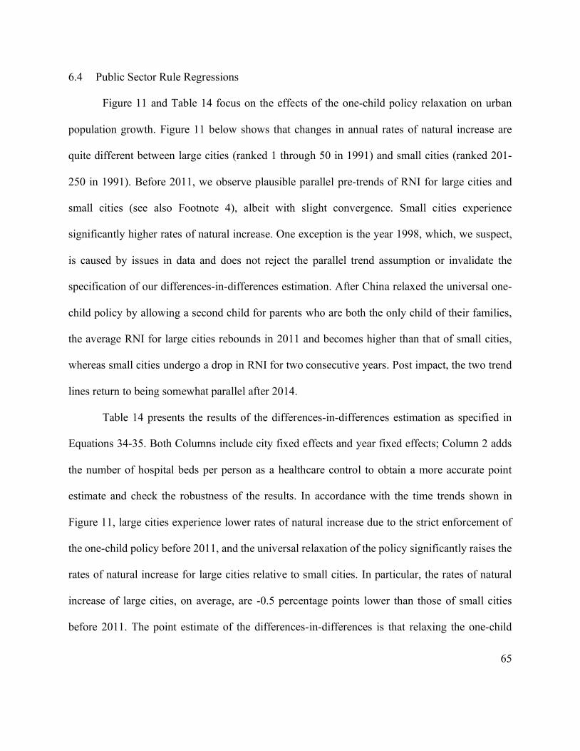
65
6.4 Public Sector Rule Regressions
Figure 11 and Table 14 focus on the effects of the one-child policy relaxation on urban
population growth. Figure 11 below shows that changes in annual rates of natural increase are
quite different between large cities (ranked 1 through 50 in 1991) and small cities (ranked 201-
250 in 1991). Before 2011, we observe plausible parallel pre-trends of RNI for large cities and
small cities (see also Footnote 4), albeit with slight convergence. Small cities experience
significantly higher rates of natural increase. One exception is the year 1998, which, we suspect,
is caused by issues in data and does not reject the parallel trend assumption or invalidate the
specification of our differences-in-differences estimation. After China relaxed the universal one-
child policy by allowing a second child for parents who are both the only child of their families,
the average RNI for large cities rebounds in 2011 and becomes higher than that of small cities,
whereas small cities undergo a drop in RNI for two consecutive years. Post impact, the two trend
lines return to being somewhat parallel after 2014.
Table 14 presents the results of the differences-in-differences estimation as specified in
Equations 34-35. Both Columns include city fixed effects and year fixed effects; Column 2 adds
the number of hospital beds per person as a healthcare control to obtain a more accurate point
estimate and check the robustness of the results. In accordance with the time trends shown in
Figure 11, large cities experience lower rates of natural increase due to the strict enforcement of
the one-child policy before 2011, and the universal relaxation of the policy significantly raises the
rates of natural increase for large cities relative to small cities. In particular, the rates of natural
increase of large cities, on average, are -0.5 percentage points lower than those of small cities
before 2011. The point estimate of the differences-in-differences is that relaxing the one-child

66
policy raises the rate of natural increase by 0.4 percentage points for large cities relative to small
cities, which is a considerable effect given that the average annual rate of natural increase for large
cities is only about 0.5 percent. It is also worth noting that the coefficient before the healthcare
control in Column 2 is positive with 99 percent statistical significance, suggesting that better
healthcare facilities have a positive partial effect on the rate of natural increase.
These results imply that the one-child policy was not uniformly enforced and, accordingly,
relaxed across China. It was more strictly enforced in cities with larger populations before 2011,
as they experienced lower rates of natural increase and thus lower birth rates if we assume death
rates to be relatively constant. It follows that, unsurprisingly, the relaxation of the one-child policy
affected large cities more positively than small cities in 2011 as the rates of natural increase for
large cities significantly increased relative to small cities. Since urban population growth consists
of natural increase and migration, we can infer that the enforcement of the one-child policy during
the 1990s and the 2000s restricted population expansion and resulted in somewhat slower urban
growth for large cities. Therefore, the different degrees to which the one-child policy was enforced
among cities provide one possible explanation for the mean reversion of city size obtained in
Section 6.2. As China gradually rescinds its one-child policy in the 2010s, we observe weaker
mean reversion than the previous two decades, as shown in Table 8 Column 4. Taking a step further,
it seems possible for large cities to catch up with small and medium-size cities on the population
growth rates in the future, which may be favorable for potential convergence to Zipf’s law.

67
Figure 11. Impact of the One-Child Policy Relaxation on Annual Rate of Natural Increase.
Note: Large cities refer to cities ranked from 1 to 50 and small cities refer to cities ranked from 151 to 200 by
population size in the year 1991. Annual Rate of Natural Increase (RNI) for each city are from NSB (1991-2017). We
take the simple average of annual RNI over all cites in the group (large or small) in any given year. 2010 represents
the last year during which China maintained the universal one-child policy before introducing a nationwide relaxation
in 2011.
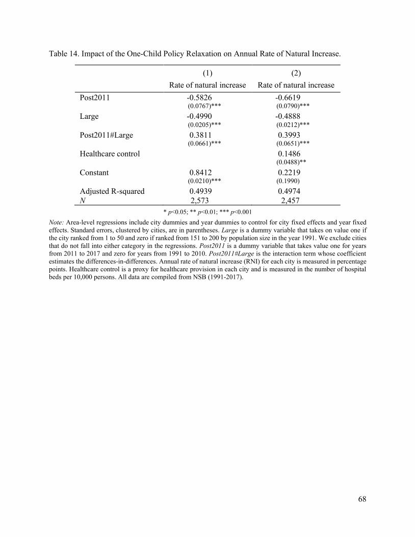
68
Table 14. Impact of the One-Child Policy Relaxation on Annual Rate of Natural Increase.
(1)
Rate of natural increase
(2)
Rate of natural increase
Post2011 -0.5826 -0.6619
(0.0767)*** (0.0790)***
Large -0.4990 -0.4888
(0.0205)*** (0.0212)***
Post2011#Large 0.3811 0.3993
(0.0661)*** (0.0651)***
Healthcare control 0.1486
(0.0488)**
Constant 0.8412 0.2219
(0.0210)*** (0.1990)
Adjusted R-squared 0.4939 0.4974
N 2,573 2,457
* p<0.05; ** p<0.01; *** p<0.001
Note: Area-level regressions include city dummies and year dummies to control for city fixed effects and year fixed
effects. Standard errors, clustered by cities, are in parentheses. Large is a dummy variable that takes on value one if
the city ranked from 1 to 50 and zero if ranked from 151 to 200 by population size in the year 1991. We exclude cities
that do not fall into either category in the regressions. Post2011 is a dummy variable that takes value one for years
from 2011 to 2017 and zero for years from 1991 to 2010. Post2011#Large is the interaction term whose coefficient
estimates the differences-in-differences. Annual rate of natural increase (RNI) for each city is measured in percentage
points. Healthcare control is a proxy for healthcare provision in each city and is measured in the number of hospital
beds per 10,000 persons. All data are compiled from NSB (1991-2017).

69
The main results on the enforcement of the hukou system are presented in Figure 12. The
scatter plots and the best linear fit lines suggest an inverse relationship between urban population
size and the unofficial migration share of the urban population. In particular, a ten percent increase
in the hukou population is associated with a 0.06 unit increase in the ratio of unofficial migrants
to hukou population. Although the magnitude of the coefficients is not as major, the negative
correlation is statistically significant, and the high values of R-squared suggest a linear relationship
is plausible. From the scatter plots, we can see that the top large cities have roughly the same
limited degrees of migration shares; small and medium-size cities, in contrast, differ greatly among
themselves, and unofficial migrants even constitute the majority of residential population in many
cities (as the ratio of unofficial migrants to hukou population is greater than one). Note that data
points with negative ratios represent a net outflow of migrants, which is the case for a handful of
medium-size cities. These observations are consistent in both census years, 2000 and 2010. Thus,
these results suggest that large cities experience greater control over unofficial migrations. As
discussed in Section 2.2, measures to achieve such stricter enforcement include limiting unofficial
migrants’ access to healthcare and education resources, housing supplies, and the local job market,
thus making it rather hard for those without hukou status to stay in the city. In addition to
minimizing unofficial migration, it is likely that large cities also issue fewer new permits each year
compared to small and medium-size cities to contain the hukou population (Zhang and Tao, 2012).
Consequently, stricter hukou control in large cities hinders urban growth both in terms of
residence-based population and in terms of hukou population, which gives us another important
policy factor that sheds light on the mean reversion of Chinese city sizes.

70
Fig
ure
12
. U
noff
icia
l M
igra
tion a
nd U
rban
Popula
tio
n S
ize,
2000
& 2
010.
N
ote
: S
ample
s re
stri
ct to
cit
ies
at p
refe
cture
lev
el a
nd a
bove. R
obust
sta
ndar
d e
rrors
are
in p
aren
thes
es. W
e ca
lcula
te t
he
num
ber
unoff
icia
l m
igra
nts
by s
ubtr
acti
ng
the
hukou p
opula
tion r
eport
ed i
n C
hin
ese
Urb
an S
tati
stic
al
Yea
rbooks
fro
m t
he
resi
den
ce-b
ased
popula
tion r
eport
ed i
n T
abula
tion o
n t
he
Popula
tion C
ensu
s of
Chin
a (
NS
B, 2000
& 2
010).

71
7 Discussion
The goal of this paper is to analyze why China’s city size distribution deviates from Zipf’s
law, and in particular, why the large cities do not grow as large as Zipf’s law predicts. First, we
find that China’s city size distribution deviates consistently from Zipf’s law over the past three
decades. In particular, the Zipf coefficient has been significantly larger than one, suggesting a more
even distribution of the population. There is some evidence suggesting potential convergence to
Zipf’s law in the most recent years from the time series plot, though this observation is sensitive
to the truncating point of our sample. Moreover, we find that the city size distribution based on
residence, which includes unofficial migrants, does not provide significantly different results from
the distribution based on hukou status in terms of the Zipf coefficient.
To explain such deviation from Zipf’s law, we find that the assumption of a homogeneous
growth process fails in Chinese cities. Instead, the urban growth rate decreases in the initial
population size whereas the variance of growth rates increases in size. These observations can
explain why the local Zipf coefficient for large cities are greater than one using Gabaix’s (1999)
general expression (Equation 7). Intuitively, the top large cities grow slower, allowing other small
or medium-size cities with higher growth rates to catch up, leading to a more even city size
distribution. This pattern of growth fits well with Chinese government’s overall urban
development strategy, which focuses on promoting growth for small and medium-size cities and
containing any further expansion of metropolitan cities. In comparison with other countries,
China’s mean reversion of city sizes appears to be much stronger, especially in the 1990s.
Concurrently, Gibrat’s law has been shown to hold in most countries, such as the United States
72
(Eeckhout, 2004; Chauvin et al., 2017), France (Eaton and Eckstein, 1997), Japan (Eaton and
Eckstein, 1997), and Brazil (Resende, 2004). Even though India also exhibits mean reversion from
1980 to 2010, the degree is much smaller with a corresponding coefficient of -0.05 (Chauvin et al.,
2017) compared to the -0.30 for China (Figure 6). Such comparison helps explain why China may
be an outlier to Zipf’s law. Another interesting finding is that China’s mean reversion becomes
weaker over time, as the regression coefficient drops to -0.07 in the 2010s and loses statistical
significance (Table 8). We may expect this trend of diminishing mean reversion to continue and
eventually support convergence to Zipf’s law.
Among our three main hypotheses for explaining why large cities experience slower urban
growth in China, namely, economic productivity slowdown, amenity deterioration, and direct
government interventions, we find that large cities are more appealing in terms of higher
productivity and better amenities, but populations grow slower due to stricter enforcement of the
one-child policy and the hukou system. Productivity and amenities are universal to other countries
in explaining urban growth patterns (Glaeser et al., 2001; Glaeser and Gottlieb, 2006). We study
how economic productivity and urban amenities connect to urban growth and population size in
China using a linear regression model and find that these two urban characteristics indeed promote
urban growth as observed in other countries, and large cities in China enjoy both higher
productivity and better amenities. The better economic performance of large cities implies that
many of the economic reforms happened during 1991-2017 benefit the large cities more than small
and medium-size cities. For instance, China’s accession to the WTO brings in more foreign capital
for large cities (see the significantly positive coefficient of 0.68 in Table 13) and opens up more
opportunities to foreign trade for large companies that mostly reside in the highly populated areas.
In addition, large cities see greater government expenditure and house price residuals, which are

73
indicators of urban amenities. As for urban issues, while large cities experience more pollution,
such disamenities are byproducts that have been overshadowed by the benefits of economic
prosperity. Thus, we do not observe any deterrence of population growth caused by crowding in
large cities. Also, China has been making special efforts to ensure better air and water quality by
moving heavy industries out of large cities like Beijing and Shanghai. Overall, it is plausible that
large cities are not yet close to their carrying capacities and still have the potential to grow further
larger given their economic well-being and social amenities. Such potential could lead to
convergence to Zipf’s law should there be free labor mobility across cities.
Finally, we justify the mean reversion of Chinese cities with government’s direct
interventions in population growth, a unique factor in China’s case. From our differences-in-
differences analysis for the one-child policy, we find that compared to small cities, large cities
suffered from lower natural increase under the universal one-child policy from 1991 to 2011 and
experienced a significant relative rise in the rate of natural increase after China’s first nationwide
relaxation of the policy in 2011, which allow parents who are both the only child to have a second
child. Likewise, our regression result of the hukou system shows that the ratio of unofficial
migrants to hukou population decreases in population size. Both results indicate that in the past,
China’s population regulations were more constraining for large cities than for small and medium-
size cities. Yet, in the most recent decade, China continues to loosen its birth planning program by
replacing the one-child policy with a universal two-child policy in 2016, whose impact may further
reduce the disadvantages in natural increase for large cities; meanwhile, China published new
regulations regarding its migration restrictions in 2014, which abolish the official distinction
between agriculture and non-agricultural hukou and extend more social welfare to unofficial

74
migrants living in the cities. As China reduces the intensity of its direct population control through
these reforms, future convergence of city sizes to Zipf’s law may be expected.
One avenue for further research on China’s population policies and city sizes is an
exploration into the effect of China’s migration control on the economic units of cities. Since
China’s heavy population regulations are imposed within the administrative boundary of each city,
many satellite towns emerge around large cities in recent years, and new migrants move to these
border towns to take advantage of the positive spillover effects of the neighboring city and
circumvent issues with official permits. This new phenomenon leads to the question of how
effective migration control really is. One may construct metropolitan areas for China using
commuting data or night lights data and examine whether the size dependency of the enforcement
intensity of the hukou system that we observe using administrative units is salient in metropolitan
areas as well. If that is the case, then China’s migration control has a far-reaching effect on
migration behaviors and population distribution beyond administrative purposes. Yet, given that
China’s lights-based metropolitan areas obey Zipf’s law (Dingel et al., 2019), we might suspect
that the hukou system is effective only in constraining population growth within administrative
boundaries but fails to impede the formation of ultra-large urban agglomerations.

75
8 Appendix
Table a. 1. Values of Zipf Coefficients, 1949-2017.
Year Zipf Coefficient Standard Error R-Squared
2017 1.061 0.068 0.846
2016 1.075 0.069 0.847
2015 1.179 0.051 0.896
2014 1.211 0.050 0.905
2013 1.232 0.049 0.914
2012 1.236 0.049 0.918
2011 1.242 0.049 0.916
2010 1.259 0.049 0.919
2009 1.248 0.050 0.912
2008 1.246 0.051 0.910
2007 1.259 0.050 0.915
2006 1.256 0.050 0.914
2005 1.244 0.050 0.915
2004 1.259 0.051 0.913
2003 1.258 0.050 0.914
2002 1.282 0.051 0.918
2001 1.321 0.051 0.921
2000 1.358 0.051 0.925
1999 1.322 0.054 0.920
1998 1.309 0.057 0.913
1997 1.295 0.061 0.903
1996 1.274 0.064 0.894
1995 1.286 0.068 0.893
1994 1.275 0.070 0.884
1993 1.274 0.067 0.898
1992 1.284 0.069 0.898
1991 1.249 0.070 0.892
1990 1.243 0.070 0.892
1989 1.231 0.069 0.892
1988 1.214 0.068 0.891
1987 1.180 0.069 0.887
1986 1.198 0.072 0.883
1985 1.228 0.077 0.882
1984 1.194 0.078 0.888
1978 1.066 0.103 0.845
1865 0.959 0.089 0.881
1957 0.977 0.089 0.891
1949 0.944 0.076 0.916
Note: Regression specifications and standard errors are based on Gabaix and Ibragimov (2011). Samples restrict to
cities at prefecture level and above in each year.
Source: Author’s calculation using population data from NSB (2000, 1984-2017).

76
Figure a. 1. Illustration of the Four Economic Regions of China.
Source: Author’s compilation.

77
Figure a. 2. Zipf’s Law: Urban Population and Urban Population Ranks (Largest 100 Cities).
Note: Regression specifications and standard errors are based on Gabaix and Ibragimov (2011). Samples restrict to
cities at prefecture level and above. Population data are from NSB (various years) measured in 10,000s.
1949 1991
2005 2017

78
Figure a. 3. Zipf Coefficients for the Four Economic Regions, 1949-2017.
Note: Regression specifications and standard errors are based on Gabaix and Ibragimov (2011). Samples restrict to
cities at prefecture level and above in each year. Population data are from NSB (various years) measured in 10,000s.
The horizontal line at 1 indicates convergence to Zipf’s law.
Central Northeastern
Western Eastern

79
Fig
ure
a.
4. A
ver
age
Wag
e an
d P
opula
tion S
ize,
201
7.
Note
: S
ample
res
tric
ts to
cit
ies
at p
refe
cture
lev
el a
nd a
bove.
Robust
sta
ndar
d
erro
rs ar
e in
par
enth
eses
. P
opula
tion dat
a ar
e m
easu
red in
10,0
00s
and
aver
age
wag
e m
easu
red i
n C
hin
ese
Yuan
. A
ll d
ata
are
from
NS
B (
2017).
Fig
ure
a.
5. A
ver
age
House
Pri
ce a
nd P
opula
tion S
ize,
2017.
N
ote
: S
ample
res
tric
ts to c
itie
s at
pre
fect
ure
lev
el a
nd a
bove.
Robust
sta
ndar
d
erro
rs a
re in p
aren
thes
es. P
opula
tion d
ata
are
from
NS
B (
2017)
and m
easu
red
in 1
0,0
00s.
House
pri
ce d
ata
are
com
pil
ed f
rom
CR
EA
(2017)
and m
easu
red
in C
hin
ese
Yuan
per
squar
e m
eter
.

80
Figure a. 6. House Price and Wage, 2017.
Note: Sample restricts to cities at prefecture level and above. Robust standard errors are in parentheses. Data on
average wages are from NSB (2017) and measured in Chinese Yuan. House prices are from CREA (2017) and
measured in Chinese Yuan per square meter.

81
9 Reference
Anderson, G., & Ge, Y. (2005). The Size Distribution of Chinese Cities. Regional Science and
Urban Economics, 35(6), 756-776.
Arshad, S., Hu, S., & Ashraf, B. (2018). Zipf’s Law and City Size Distribution: A Survey of the
Literature and Future Research Agenda. Physica A: Statistical Mechanics and Its
Applications, 492, 75-92.
Auerbach, F. (1913). Das Gesetz der Bevölkerungskonzentration. Petermann's Mitteilungen, 59,
74–76.
Bacolod, M., Blum, B., & Strange, W. (2009). Skills in the City. Journal of Urban Economics,
65(2), 136-153.
Chauvin, J., Glaeser, E., Ma, Y., & Tobio, K. (2017). What is Different about Urbanization in Rich
and Poor Countries? Cities in Brazil, China, India and the United States. Journal of Urban
Economics, 98(C), 17-49.
Chen, Z., Fu, S., & Zhang, D. (2013). Searching for the Parallel Growth of Cities in China. Urban
Studies, 50(10), 2118-2135.
CREA (China Real Estate Association). (2017). China Housing Price Data. Big Data Platform of
Chinese Real Estate. Retrieved from https://www.creprice.cn/solution/a_platform.html.
Dingel, J., Miscio, A., & Davis, D. (2019). Cities, Lights, and Skills in Developing Economies.
Journal of Urban Economics.

82
Eaton, J., & Eckstein, Z. (1997). Cities and Growth: Theory and Evidence from France and Japan.
Regional Science and Urban Economics, 27(4), 443-474.
Eeckhout, J. (2004). Gibrat’s Law for (All) Cities. American Economic Review, 94(5), 1429-1451.
Fang, L., Li, P., & Song, S. (2017). China’s Development Policies and City Size Distribution: An
Analysis based on Zipf’s Law. Urban Studies, 54(12), 2818-2834.
Gabaix, X. (1999). Zipf's Law for Cities: An Explanation. The Quarterly Journal of Economics,
114(3), 739-767.
Gabaix, X., & Ibragimov, R. (2011). Rank − 1 / 2: A Simple Way to Improve the OLS Estimation
of Tail Exponents. Journal of Business & Economic Statistics, 29(1), 24-39.
Gangopadhyay, K., & Basu, B. (2009). City Size Distributions for India and China. Physica A:
Statistical Mechanics and Its Applications, 388(13), 2682-2688.
Gangopadhyay, K., & Basu, B. (2012). Evolution of Zipf’s Law for Indian Urban Agglomerations
Vis-à-vis Chinese Urban Agglomerations. ArXiv.org, 13, 119-129.
Glaeser, E. (2008). Cities, Agglomeration, and Spatial Equilibrium (Lindahl lectures). New York:
Oxford University Press.
Glaeser, E., & Gottlieb, J. (2009). The Wealth of Cities: Agglomeration Economies and Spatial
Equilibrium in the United States. Journal of Economic Literature, 47(4), 983-1028.
Glaeser, E., & Gottlieb, J. (2006). Urban Resurgence and the Consumer City. Urban Studies, 43(8),
1275-1299.

83
Glaeser, E., Kolko, J., & Saiz, A. (2001). Consumer City. Journal of Economic Geography, 1(1),
27-50.
Glaeser, E., Scheinkman, J., & Shleifer, A. (1995). Economic Growth in a Cross-Section of Cities.
Journal of Monetary Economics, 36(1), 117-143.
Gibrat, R. (1931). Les Inégalités Économiques. Paris: Recueil Sirey.
Giesen, K., & Südekum, J. (2011). Zipf’s Law for Cities in the Regions and the Country. Journal
of Economic Geography, 11(4), 667-686.
González-Val, R. (2010). The Evolution of U.S. City Size Distribution from a Long-Term
Perspective (1900–2000). Journal of Regional Science, 50(5), 952-972.
González-Val, R., Lanaspa, L., & Sanz-Gracia, F. (2014). New Evidence on Gibrat’s Law for
Cities. Urban Studies, 51(1), 93-115.
Gu, E. (2002). The State Socialist Welfare System and the Political Economy of Public Housing
Reform in Urban China. Review of Policy Research, 19(2), 179-211.
Gyourko, J. & Tracy, J. (1991). The Structure of Local Public Finance and the Quality of Life. The
Journal of Political Economy, 99(4), 774-806.
Holmes, T. & Lee, S. (2010). Cities as Six-by-Six-Mile Squares: Zipf’s Law? In E. Glaeser,
(Eds.), Agglomeration Economics (pp. 105-131). University of Chicago Press.
Ioannides, Y., & Overman, H. (2003). Zipf’s Law for Cities: An Empirical Examination. Regional
Science and Urban Economics, 33(2), 127-137.

84
Ioannides, Y., & Skouras, S. (2013). US City Size Distribution: Robustly Pareto, but Only in the
Tail. Journal of Urban Economics, 73(1), 18-29.
Krugman, P. (1996). The Self-Organizing Economy. Malden, MA: Blackwell.
Li, H., Wei, Y., & Ning, Y. (2016). Spatial and Temporal Evolution of Urban Systems in China
during Rapid Urbanization. Sustainability, 8(7), 651.
Li, J. (1995). China’s One-Child Policy: How and How Well Has It Worked? A Case Study of
Hebei Province, 1979-1988. Population and Development Review, 21(3), 563.
Luckstead, J., & Devadoss, S. (2014). A Comparison of City Size Distributions for China and India
from 1950 to 2010. Economics Letters, 124(2), 290-295.
Matlaba, V., Holmes, M., McCann, P., & Poot, J. (2013). A Century of the Evolution of the Urban
System in Brazil. Review of Urban & Regional Development Studies, 25(3), 129-151.
Mills, E. (1967). An aggregative model of resource allocation in a metropolitan area. American
Economic Review, 57(2), 197-210.
Moretti, E. (2003). Human Capital Externalities in Cities. NBER Working Paper Series, 9641.
Moura, N., & Ribeiro, M. (2013). Testing the Goodwin Growth-Cycle Macroeconomic Dynamics
in Brazil. Physica A: Statistical Mechanics and Its Applications, 392(9), 2088-2103.
NSB (National Bureau of Statistics). (1984-2017). Chinese Urban Statistical Yearbooks. Beijing:
China Statistical Press.
NSB. (2000). Fifty Years of Urban Development. Beijing: China Statistical Press.
85
NSB. (2000 & 2010). Tabulation on the Population Census of China. Beijing: China Statistical
Press.
Pasciuti, D. (2014). Reexamining Zipf’s Law from a World Historical Perspective: Urbanization,
Complexity, and the Rank-Size Rule. The International Journal of Interdisciplinary Global
Studies, 7(4), 29-40.
Peng, G. (2010). Zipf’s Law for Chinese Cities: Rolling Sample Regressions. Physica A: Statistical
Mechanics and Its Applications, 389(18), 3804-3813.
Rastvortseva, S., & Manaeva, I. (2019). Estimation of Temporal Growth Rate of Russian Cities.
Regional Economics: Theory and Practice, 17(3), 402-417.
Resende, M. (2004). Gibrat’s Law and the Growth of Cities in Brazil: A Panel Data Investigation.
Urban Studies, 41(8), 1537-1549.
Singer, H. (1936). The “Courbe des Populations.” A Parallel to Pareto's Law. The Economic
Journal, 46(182), 254-263.
Song, S., & Zhang, K. (2002). Urbanisation and City Size Distribution in China. Urban Studies,
39(12), 2317-2327.
Song, Y. (2014). What Should Economists Know about the Current Chinese Hukou System?
China Economic Review, 29, 200-212.
Wu, J., & He, L. (2017). How Do Chinese Cities Grow? A Distribution Dynamics Approach.
Physica A: Statistical Mechanics and Its Applications, 470(C), 105-118.

86
Xu, Z., & Zhu, N. (2009). City Size Distribution in China: Are Large Cities Dominant? Urban
Studies, 46(10), 2159-2185.
Zhang, L. & Tao, L. (2012). Barriers to the Acquisition of Urban Hukou in Chinese Cities.
Environment and Planning A, 44(12), 2883-2900.
Zipf, G. (1949). Human Behavior and the Principle of Least Effort: An Introduction to Human
Ecology. Cambridge, Mass.: Addison-Wesley Press.
Recommended