AN ECONOMETRIC ANALYSIS OF
AUSTRALIAN DOMESTIC TOURISM
DEMAND
Ghialy Choy Lee Yap
2010
Doctor of Philosophy

ii
Use of Thesis
This copy is the property of Edith Cowan University. However, the literary rights of the
author must also be respected. If any passage from this thesis is quoted or closely
paraphrased in a paper of written work prepared by the user, the source of the passage
must be acknowledged in the work. If the user desires to publish a paper or written work
containing passages copied or closely paraphrased from this thesis, which passages
would in total constitute an infringing copy for the purpose of the Copyright Act, he or
she must first obtain the written permission of the author to do so.

iii
A Statement of Confidential
Information
I, Ghialy Yap, have accessed information which is provided by Tourism Research
Australia, the Australian Bureau of Statistics and the Reserve Bank of Australia for the
purpose of undertaking research and writing a thesis. The data employed are available in
the websites of the above-mentioned government agencies.
In Chapter 4 of this thesis, the tourism data used in the tables and graphs are extracted
from the quarterly reports of Travel by Australians, from March 1999 to December
2007, by Tourism Research Australia in Canberra. Copyright 2010 Commonwealth of
Australia reproduced by permission.
Signed by,
______________________
Ghialy Choy Lee Yap
PhD Scholar
Faculty of Business and Law
Edith Cowan University
Date: 5th
March 2010

iv
Preface
Several parts of this PhD research have been accepted for journal publications and
academic conferences, as follows.
(i) “Modelling interstate tourism demand in Australia: A cointegration analysis”,
Mathematics and Computers in Simulation vol. 79 (2009) pp. 2733-2740.
(ii) “An empirical analysis of interstate and intrastate tourism demand in
Australia”, a peer-reviewed conference paper in the 2007 CAUTHE
Conference.
(iii) “Modelling Australian domestic tourism demand: A panel data analysis”, a
peer-reviewed conference paper for the 18th
IMACS World Congress-
MODSIM09 International Congress on Modelling and Simulation.
(iv) “Investigating other factors influencing Australian domestic tourism
demand”, a peer-reviewed conference paper for the 18th
IMACS World
Congress-MODSIM09 International Congress on Modelling and Simulation.

v
Abstract
In 2007, the total spending by domestic visitors was AUD 43 billion, which was 1.5
times higher than the aggregate expenditure by international tourists in Australia.
Moreover, domestic visitors consumed 73.7% of the Australian produced tourism goods
and services whereas international tourists consumed 26.3%. Hence, this shows that
domestic tourism is an important sector for the overall tourism industry in Australia.
This present research determines the factors that influence domestic tourism demand in
Australia and examines how changes in the economic environment in Australia could
influence this demand. The main aim of this research is to achieve sustainability of
domestic tourism businesses in Australia.
In Chapters Two and Three, a review of the tourism demand literature is conducted.
Most of the empirical papers argued that household income and travel prices are the
main demand determinants. However, the literature has largely neglected other possible
indicators, namely consumers‟ perceptions of the future economy, household debt and
working hours, which may play an important role in influencing domestic tourism
demand in Australia.
The PhD thesis is divided into three parts. For the initial phase, a preliminary study is
conducted using Johansen‟s cointegration analysis to examine the short- and long-run
coefficients for the determinants of Australian domestic tourism demand. In the next
section of this thesis, an alternative approach using panel data analysis to estimate the
income and price elasticities of the demand is applied, as a panel data framework
provides more information from the data and more degrees of freedom. In the final
section, this thesis also investigates whether other factors (such as the consumer
sentiment index, and measures of household debt and working hours) influence
Australians‟ demand for domestic trips.
This study reveals several distinct findings. First, the income elasticity for domestic
visitors of friends and relatives (VFR) and interstate trips is negative, implying that
Australian households will not choose to travel domestically when there is an increase
in household income. In contrast, the study finds that the income variables are positively

vi
correlated with domestic business tourism demand, indicating that the demand is
strongly responsive to changes in Australia‟s economic conditions. Second, an increase
in the current prices of domestic travel can cause the demand for domestic trips to fall in
the next one or two quarters ahead. Third, the coefficients for lagged dependent
variables are negative, indicating perhaps, that trips are made on a periodic basis.
Finally, to a certain extent, the consumer sentiment index, household debt and working
hours have significant influences on domestic tourism demand.
The current econometric analysis has significant implications for practitioners. A better
understanding of income and travel cost impacts on Australian households‟ demand
allows tourism companies to develop price strategies more effectively. Moreover,
tourism researchers can use these indicators (such as measures of consumers‟
confidence about their future economy, household debt and working hours) to
investigate how changes in these factors may have an impact on individual decisions to
travel.

vii
Declaration
I certify that this thesis does not, to the best of my knowledge and belief:
(i) incorporate without acknowledgement any material previously submitted for
a degree of diploma in any institution of higher education;
(ii) contain any material previously published or written by another person
except where due reference is made in the text; or
(iii) contain any defamatory material.
I also grant permission for the library at Edith Cowan University to make duplicate
copies of my thesis as required.
Signed by,
_________________________
Ghialy Choy Lee Yap
PhD Scholar
Faculty of Business and Law
Edith Cowan University
Date: 5th
March 2010

viii
Acknowledgements
The journey from the beginning to the completion of this thesis was full of challenges,
but the experience was rewarding. I encountered many nice and kind people who gave
me good advice and courage to go through this journey. Hence, this thesis would not be
completed successfully without their support.
First and foremost, I would like to thank my principal supervisor, Professor David
Allen, for his emotional support and sharp intellect. As English is not my first language,
he always listened to my queries with empathy and explained his ideas and comments
patiently. More importantly, I am indebted to his time and efforts for editing numerous
versions of my thesis. I would also like to thank my associate supervisor, Dr. Riaz
Shareef, who has a high level of knowledge in tourism literature. I am gratitude for his
guidance in constructing the literature review chapters, and his motivating conversations
whenever I was depressed.
Since the commencement of my PhD candidature, I have been in receipt of a Three-and-
a half years joint scholarship from Sustainable Tourism Cooperative Research Centre
(STCRC) and Edith Cowan University (ECU). This scholarship has supported my life
throughout the candidature. Given this opportunity, I would like to thank Professor
Beverly Sparks, the Director of the STCRC education program, and Professor Marilyn
Clark-Murphy, the Head of School (in 2006), for granting this scholarship for my
research project.
I would like to dedicate my thanks to Dr. Greg Maguire and Dr. Jo Mcfarlane (the
writing consultants), who provided guidance on my English writing styles and grammar.
Similarly, I would like to thank Associate Professor Zhaoyong Zhang and Dr. Lee Kian
Lim for providing positive criticisms of my research proposals. Also, I am grateful to
several ECU staff: To Kathryn Peckham, who did an excellent job in maintaining good
conditions of the office facilities for postgraduate students and in handling my
scholarship issues; to Sue Stenmark and Sharron Kent (then), who were efficient in
dealing with my conference travelling expenses; as well as to Dr. Susan Hill, who

ix
organised research training programs and workshops for postgraduate students at the
university.
During my PhD years, I was very fortunate to be able to travel and present my research
in international academic conferences. The travel experience was priceless as I had the
best opportunities to network with senior researchers from around the world. I would
like to acknowledge STCRC and ECU for funding my conference travelling expenses.
Also, I would like to express my appreciation to Professor Christine Lim, Professor
Lindsay Turner, Associate Professor Kevin Wong, anonymous paper reviewers and
other conference participants, for contributing their useful comments.
I would like to thank Erin Boyce from Tourism Research Australia, for her excellent
customer service in providing domestic tourism datasets. Also, I am grateful to Dr.
Suhejla Hoti who gave me good advice on how to construct my research topic.
I am indebted to my close friends who had shown their compassion throughout the
journey. Especially, I would like to thank Dr. Abdul Hakim for his positive thinking,
great sense of humour, kindness, and encouraging words. I could not have completed
this thesis without all the support he gave me. I am also grateful to Anthony Chan,
Alfred Ogle, Daphnie Goh, Dr. Duc Vo, Imbarine Bujang, Mandy Pickering, Meiyan
Wong, Michelle Rowe, Dr. Mun Woo, Sharon Tham, Yiwei Ang and Thameena
Khares, my colleagues and friends who had been giving their continuous support and
advice.
Last but not least, I would like to dedicate my special thanks to my parents, my
grandmother and my sister. Their unconditional love and tolerance have earned my
respect. Especially my parents, my mom has been travelling to Perth occasionally to
visit and accompany me; and my dad always reminded me to enjoy whatever I do. As
for my beloved sister, she always called and asked about me despite that she was busy
with her job in Malaysia. Thank you for being so supportive.

x
Table of Contents
List of Tables…………………………………………………………………………xiii
List of Figures………………………………………………………………………..xvii
Chapter 1 Introduction
1.1 The impacts of tourism on the Australian economy: An overview ......................... 1
1.2 Tourism development in Australia........................................................................... 3
1.2.1 Promoting and marketing Australian tourism ................................................... 4
1.2.2 Developing new tourism markets ..................................................................... 4
1.2.3 Expanding tourism businesses .......................................................................... 5
1.2.4 Upgrading the transport and infrastructure facilities ........................................ 6
1.3 The importance of domestic tourism in Australia.................................................... 6
1.4 Australian domestic tourism demand: its challenges ............................................... 8
1.5 An overview of this thesis...................................................................................... 11
Chapter 2 A review of the tourism demand literature
2.1 Tourism demand research: Its developments and critical issues ........................... 13
2.1.1 The application of advanced econometric techniques .................................... 13
2.1.2 Reliable disclosure of empirical findings after 1995 ...................................... 15
2.1.3 Significant dearth of empirical research on domestic tourism demand .......... 16
2.1.4 Critical issues in the domestic tourism literature ............................................ 17
2.2 Theoretical development of tourism demand drivers ............................................ 20
2.2.1 The application of consumer demand theory in modelling tourism demand.. 20
2.2.2 The use of leading economic indicators in tourism demand studies .............. 22
2.3 The study of Australian domestic tourism demand: A review of the empirical
literature ..................................................................................................... 25
2.4 Further extension of the existing literature ............................................................ 28
2.5 Conclusion ............................................................................................................. 29
Appendix 2.1 A summary of empirical research on international tourism demand......30
Appendix 2.2 A summary of empirical research on domestic tourism demand...........98

xi
Chapter 3 The determinants of domestic and international tourism: A review and
comparison of findings
3.1 Income ................................................................................................................. 120
3.2 Tourism prices ..................................................................................................... 125
3.3 Other demand determinants................................................................................. 136
3.3.1 The effects of positive and negative events ................................................. 136
3.3.2 Lagged dependent variables ......................................................................... 140
3.3.3 Destination preference index (DPI).............................................................. 142
3.3.4 Trade volume or openness to trade .............................................................. 143
3.3.5 Marketing expenditure ................................................................................. 145
3.3.6 Tourism supply ............................................................................................. 145
3.3.7 Working hours .............................................................................................. 147
3.4 Conclusion ........................................................................................................... 147
Chapter 4 Australian domestic tourism demand: Data and seasonality analyses
4.1 Introduction: Australian domestic tourism markets ............................................ 149
4.2 Domestic tourism performance by state .............................................................. 156
4.2.1 Australian Capital Territory (ACT).............................................................. 157
4.2.2 New South Wales (NSW) ............................................................................ 160
4.2.3 Northern Territory (NT) ............................................................................... 167
4.2.4 Queensland (QLD) ....................................................................................... 172
4.2.5 South Australia (SA) .................................................................................... 177
4.2.6 Tasmania (TAS) ........................................................................................... 182
4.2.7 Victoria (VIC) .............................................................................................. 188
4.2.8 Western Australia (WA)............................................................................... 193
4.3 Conclusion ........................................................................................................... 198
Chapter 5 Modelling Australian domestic tourism demand (I): A preliminary
study
5.1 Motivation ........................................................................................................... 201
5.2 Modelling Interstate Domestic Tourism Demand in Australia ........................... 201
5.2.1 Unit root tests .................................................................................................... 203
5.2.2 Cointegration analysis ....................................................................................... 204

xii
5.3 An empirical analysis of domestic intrastate and interstate tourism demand in
Australia ................................................................................................... 210
5.4 Conclusion ........................................................................................................... 216
Chapter 6 Modelling Australian domestic tourism demand (II): A panel data
approach
6.1 Motivation ............................................................................................................ 219
6.2 Estimation of Australian domestic tourism demand ............................................ 219
6.3 Panel unit root tests .............................................................................................. 223
6.4 Panel data static regressions................................................................................. 226
6.5 Panel data dynamic models .................................................................................. 240
6.6 Investigating other related factors affecting Australian domestic tourism demand
.................................................................................................................. 243
6.7 Cdonclusion ......................................................................................................... 256
Chapter 7 Conclusion: Discussion, limitation and implications
7.1 Introduction .......................................................................................................... 260
7.2 Discussion ............................................................................................................ 260
7.3 Limitations ........................................................................................................... 262
7.4 Future directions .................................................................................................. 264
References....................................................................................................................268

xiii
List of Tables
Table 1.1 Real tourism gross value added (GVA) in each Australian State for
the year ended 30 June 2007.................................................................. 2
Table 1.2 The share of tourism income relative to total state income in each
Australian State for the year ended 30 June 2007.................................. 2
Table 1.3 Number of persons employed in tourism-related industries („000),
2004-2007.............................................................................................. 3
Table 1.4 Domestic international visitors in Australia, 2000-2003....................... 7
Table 1.5 Average contribution of tourist expenditure to each person employed,
2004-2007.............................................................................................. 8
Table 1.6 Domestic and outbound visitors in Australia, 2004-2007...................... 9
Table 1.7 Forecast of the growth of domestic visitor nights and Australians
travelled overseas for the year 2010-2016............................................. 9
Table 1.8 Main indicators of the Australian economy for 2000 and 2006............ 10
Table 3.1 Income elasticities of international tourism demand............................. 121
Table 3.2 Income elasticities of domestic tourism demand................................... 125
Table 3.3 Relative price elasticities of international tourism demand................... 127
Table 3.4 Exchange rate elasticities of international tourism demand................... 130
Table 3.5 Transportation cost elasticities of international tourism demand.......... 131
Table 3.6 Substitute price elasticities of international tourism demand................ 133
Table 3.7 Tourism price elasticities of domestic tourism demand........................ 135
Table 3.8 Effects of negative events on international tourism demand................. 138
Table 3.9 Effects of positive events on international tourism demand.................. 139
Table 3.10 Effects of negative and positive events on domestic tourism demand.. 139
Table 3.11 Coefficients of the lagged dependent variable in international tourism
demand studies....................................................................................... 140
Table 3.12 Coefficients of lagged dependent variable in domestic tourism
demand................................................................................................... 142
Table 3.13 Coefficients of destination preference index in international tourism
demand studies....................................................................................... 143
Table 3.14 Coefficients of trave volume in international tourism demand studies. 144
Table 3.15 Coefficients of marketing expenditure in international tourism
demand studies....................................................................................... 145
Table 3.16 Coefficients of tourism supply in international tourism demand
studies..................................................................................................... 146
Table 3.17 Coefficients of working hours in domestic tourism demand studies..... 147

xiv
Table 4.1 Top ten ranking of the most consumed Australian household items,
2006-2007.............................................................................................. 150
Table 4.2 Domestic visitor nights in Australia from 2005 to 2008, by purpose of
visits....................................................................................................... 151
Table 4.3 Average expenditure per domestic visitor night from 2005 to 2008,
by purpose of visits................................................................................ 151
Table 4.4 Domestic day visitors in Australia from 2005 to 2008, by purpose of
visits....................................................................................................... 152
Table 4.5 Average expenditure per domestic overnight and day visitors from
2005 to 2008, by purpose of visits (AUD)............................................. 154
Table 4.6 Descriptive statistics of domestic visitor nights („000) in ACT for
quarterly data from 1999 to 2007.......................................................... 158
Table 4.7 Visitor nights („000) in ACT by purpose of visits in each quarter........ 160
Table 4.8 Descriptive statistics of domestic tourist markets in NSW („000)......... 162
Table 4.9 Average domestic tourism demand in NSW in each quarter of the
year („000).............................................................................................. 166
Table 4.10 Descriptive statistics of domestic tourist markets in NT („000)............ 167
Table 4.11 Average domestic tourism demand in NT in each quarter of the year
(„000)...................................................................................................... 172
Table 4.12 Descriptive statistics of domestic tourist markets in QLD („000)......... 173
Table 4.13 Average domestic tourist demand in QLD in each quarter of the year
(„000)...................................................................................................... 177
Table 4.14 Descriptive statistics of domestic tourist markets in SA („000)............. 178
Table 4.15 Average domestic tourism demand in SA in each quarter of the year
(„000)...................................................................................................... 182
Table 4.16 Descriptive statistics of domestic tourist markets in TAS („000).......... 183
Table 4.17 Average domestic tourism demand in TAS in each quarter of the year
(„000)...................................................................................................... 188
Table 4.18 Descriptive statistics of domestic tourist markets in VIC („000)........... 189
Table 4.19 Average domestic tourism demand in VIC in each quarter of the year
(„000)...................................................................................................... 193
Table 4.20 Descriptive statistics of domestic tourist markets in WA („000)........... 194
Table 4.21 Average domestic tourism demand in WA in each quarter of the year
(„000)...................................................................................................... 198
Table 4.22 A summary of domestic overnight tourism demand in each Australian
States...................................................................................................... 199
Table 5.1 Unit root test statistics for economic variables in logarithms................ 204
Table 5.2 Unit root test statistics for economic variables in log-differences......... 204
Table 5.3 Test statistics for the length of lags of VAR model............................... 207
xv
Table 5.4 Cointegration test................................................................................... 207
Table 5.5 Error-correction model........................................................................... 208
Table 5.6 Long-run coefficients for interstate tourism demand............................. 209
Table 5.7 A summary results of model specification, the significance of error
correction term and diagnostic tests....................................................... 213
Table 5.8 Estimated short-run coefficients............................................................ 214
Table 5.9 Estimated long-run coefficients............................................................. 216
Table 6.1 List of proxy variables........................................................................... 220
Table 6.2 IPS panel unit root test for the dependent variables.............................. 224
Table 6.3 IPS panel unit root test for the independent variables........................... 225
Table 6.4 Estimate of the double-log static panel model [Dependent variable:
Holiday visitor nights (HOL)]................................................................ 231
Table 6.5 Estimate of the double-log static panel model [Dependent variable:
Business visitor nights (BUS)................................................................ 232
Table 6.6 Estimate of the double-log static panel model [Dependent variable:
VFR visitor nights]................................................................................. 233
Table 6.7 Estimate of the double-log static panel model [Dependent variable:
OTH visitor nights]................................................................................ 234
Table 6.8 Estimate of the double-log static panel model [Dependent variable:
Interstate visitor nights (NV)]................................................................ 235
Table 6.9 Estimate of the double-log static panel model [Dependent variable:
Intrastate visitor nights (NVI)]............................................................... 236
Table 6.10 Estimate of the double-log static panel model [Dependent variable:
Number of interstate visitors (OV)]....................................................... 237
Table 6.11 Estimate of the double-log static panel model [Dependent variable:
Number of intrastate visitors (OVI)]...................................................... 238
Table 6.12 Estimate of the double-log panel model with dynamic [Dependent
variable: Holiday visitor nights (HOL)]................................................. 243
Table 6.13 Estimate of the double-log panel model with dynamic [Dependent
variable: Business visitor nights (BUS)]................................................ 244
Table 6.14 Estimate of the double-log panel model with dynamic [Dependent
variable: VFR visitor nights]………….................................................. 245
Table 6.15 Estimate of the double-log panel model with dynamic [Dependent
variable: OTH visitor nights]…………................................................. 246
Table 6.16 Estimate of the double-log panel model with dynamic [Dependent
variable: Interstate visitor nights (NV)]................................................. 247
Table 6.17 Estimate of the double-log panel model with dynamic [Dependent
variable: Intrastate visitor nights (NVI)]................................................ 248
Table 6.18 Estimate of the double-log panel model with dynamic [Dependent
variable: Number of interstate visitors (OV)]........................................ 249
xvi
Table 6.19 Estimate of the double-log panel model with dynamic [Dependent
variable: Number of intrastate visitors (OVI)]....................................... 250
Table 6.20 List of additional variable used……………………………………….. 252
Table 6.21 Empirical results of Australian domestic tourism demand……..…….. 257

xvii
List of Figures
Figure 4.1 Visitor expenditure in each State/Territory for the year ended 31
March 2008………………………………………………………….. 155
Figure 4.2 Visitor nights by purpose of visits in ACT………………………….. 159
Figure 4.3 Numbers of visitor nights by purpose of visits and numbers of
interstate and intrastate visitors in NSW……………………………. 162
Figure 4.4 Numbers of visitor nights by purpose of visits and numbers of
interstate and intrastate visitors in NT………………………………. 168
Figure 4.5 Numbers of visitor nights by purpose of visits and numbers of
interstate and intrastate visitors in QLD..…………………………. 174
Figure 4.6 Numbers of visitor nights by purpose of visits and numbers of
interstate and intrastate visitors in SA………………………………. 179
Figure 4.7 Numbers of visitor nights by purpose of visits and numbers of
interstate and intrastate visitors in TAS..……………………………. 184
Figure 4.8 Numbers of visitor nights by purpose of visits and numbers of
interstate and intrastate visitors in VIC..……………………………. 190
Figure 4.9 Numbers of visitor nights by purpose of visits and numbers of
interstate and intrastate visitors in WA…………..…………………. 195


1
Chapter 1 Introduction
1.1 The impacts of tourism on the Australian economy: An overview
Tourism in Australia has grown strongly over the past ten years. Tourism gross value
added1 (GVA) has climbed gradually from AUD22 billion in 1998 to AUD31 billion in
2006, implying that tourism producers in Australia have increased their production of
goods and services by 43%. Furthermore, the gross domestic product for the tourism
industry (or tourism GDP2) generated AUD38 billion in 2006, which was a rise of 53%
compared to 1998.
In addition, the tourism industry in each Australian State has performed well in 2007.
Table 1.1 reveals that all Australian States have shown positive growth in real tourism
GVA. In particular, real tourism GVA in Western Australia has shown the most
significant growth. Moreover, the table shows that New South Wales, Victoria and
Queensland generated the highest values of real tourism GVA, indicating that tourism is
one of the important sources of revenue for these states.
Table 1.2 exhibits the share of tourism revenue relative to total state income in each
Australian State. In 2007, Queensland recorded the highest share of tourism income, in
which the income source was mostly generated from its famous theme parks as well as
sun and beach destinations, such as Brisbane, the Gold Coast and the Sunshine Coast.
However, the share of tourism revenue in Queensland grew less than 1% in 2007
compared to 1998, indicating that tourism in Queensland has become a mature tourism
product in Australia. Table 1.2 also shows that tourism in South Australia, Tasmania
and Victoria have contributed significantly to state income. Particularly for Victoria and
South Australia, the tourism revenue shares in 2007 have increased by 12.31% and
12.07%, respectively (Table 1.2).
1 Tourism GVA shows the value of output in tourism industry minus the input used to produce the output.
It indicates how much extra tourism goods and services have been produced by Australian tourism
producers. 2 Tourism GDP measures the value added of the tourism industry at purchasers‟ (market) prices. The
difference between tourism GDP and GVA is that the output value for GDP includes any taxes and/or
subsidies on tourism products whereas the output value for GVA excludes them.

2
Table 1.1. Real tourism gross value added (GVA) in each Australian State for the year
ended 30 June 2007
State Real tourism GVA
(AUD billion) % change
Australian Capital Territory 2.31 3.26
Northern Territory 1.64 4.67
Tasmania 2.99 3.86
Western Australia 15.49 8.07
South Australia 9.15 3.53
Queensland 30.85 4.09
Victoria 32.11 4.53
New South Wales 43.90 3.68
Note: Real tourism GVA (RGVA) is the net value of output in tourism industry after adjusted
with inflation rate. The % change is based on the equation:
% change = RGVA(t) − RGVA(t − 1)
RGVA(t − 1) × 100
where t = time. It measures by how much the current RGVA has changed compared to previous
year. The data above are extracted from the Australian National Accounts: State Accounts 2006-
07(Cat. No.: 5220.0), the Australian Bureau of Statistics (ABS).
Table 1.2. The share of tourism income relative to total state income in each Australian
State for the year ended 30 June 2007
State Share of tourism income to
total state income (%) % change since June 1998
Australian Capital Territory 11 -4.18
Northern Territory 12.21 -5.86
Tasmania 15.52 9.14
Western Australia 12.12 1.00
South Australia 13.93 12.07
Queensland 16.47 0.67
Victoria 13.23 12.31
New South Wales 13.66 3.96
Note: Tourism income is calculated based on the revenue earned in the selected tourism-related
industries, namely accommodation, cafes and restaurants, cultural and recreational services, and
transport and storage. The share of tourism income to total state income is the ratio of tourism
income and the overall state revenue, and the ratio is expressed in percentage. The % change is
computed to measure how much the ratio has increased or decreased since 1998. All data are
extracted from the Australian National Accounts: State Accounts 2006-07 (Cat. No.: 5220.0),
ABS.

3
In addition, employment opportunities in tourism have increased steadily over the last
four years. Compared to 2004, the number of persons employed in the tourism sectors
has risen about 6.8% in 2007 (Table 1.3). Within the industry itself, the retail trade
employed the highest number of staff. Furthermore, there was a gradual growth in job
opportunities in transport and storage, and cultural and recreation services during 2004
and 2007. For the accommodation, café and restaurants sectors, there was a decline of
4.3% in the number of persons employed in 2006; but in the following year, the job
opportunities in these sectors surged by approximately 5.6%.
Table 1.3. Number of persons employed in tourism-related industries („000), 2004-2007
Year Retail trade Accommodation,
café and
restaurants
Transport and
storage
Cultural and
recreation
services
Total persons
employed in
tourism
2004 1,436.5 469.1 431.7 238.8 2,576.1
2005 1,485.9 501.4 453.6 260.2 2,701.1
2006 1,497.9 479.9 461.4 274.3 2,713.5
2007 1,492.5 506.9 471.0 280.6 2,751.0
Note: The source of data is obtained from the Labour Force, Australia (Cat. No.:
6291.0.55.003), ABS. The figures are based on the annual time-series data for the employed
persons by industry. The data on total persons employed in tourism industry are the summation
of people employed in tourism-related industries, namely retail trade, accommodation, cafe and
restaurants, transport and storage, and cultural and recreation services.
1.2 Tourism development in Australia
Given the importance of tourism to the Australian economy, particularly in generating
job opportunities and tourism revenue, the Australian Government released the
AUD235 million Tourism White Paper (TWP) in 2003, which is a ten-year plan to
develop and sustain the tourism industry in Australia. The key contribution of the TWP
is that the government has established a new government body, Tourism Australia, to
bring together the former Australian Tourist Commission, the Bureau of Tourism
Research, See Australia and the Tourism Forecasting Council under one umbrella.
In the TWP, the government has outlined several strategies to increase awareness of
Australian tourism domestically and globally as well as to improve tourism products in
Australia. The strategies focus on four main areas, namely promoting and marketing

4
Australian tourism, developing new tourism markets, expanding tourism businesses,
and upgrading transport and infrastructure facilities.
1.2.1 Promoting and marketing Australian tourism
One of the goals in the TWP is to promote Australian tourism to domestic and
international markets. To do so, the government has provided AUD120.6 million for
funding overseas advertisement and marketing expenses. Furthermore, an additional
funding of AUD45.5 million has been allocated to implement a domestic marketing
campaign [Commonwealth of Australia (2007)].
On 23 February 2006, Tourism Australia launched an advertising campaign entitled as
“A uniquely Australian invitation” in overseas markets. The immediate effect of the
advertisement was that the visitation of the Australia website increased by 40% at the
end of 2006 compared to previous year [Tourism White Paper, Annual Progress Report
(2006)].
In addition, Tourism Australia has contributed AUD7 million for broadcasting the
uniqueness of Australia in global media channels such as the National Geographic and
Discovery channels. The main aim is to publicize Australia as a tourist destination to the
target market such as the Experience Seeker, through the partnerships with these
channels.
Apart from international marketing, Tourism Australia has launched a domestic
marketing campaign, namely “My Australia”, on 26 October 2006, in partnership with
the Seven Network in Australia. Furthermore, more advertisement campaigns have been
implemented in 2007, cooperating with the Australia‟s major publication company,
namely Fairfax. The prime purpose of such campaigns is to build awareness of the
Australian holiday experience to local residents.
1.2.2 Developing new tourism markets
In the announcement of the 2006-07 Budget, the Australian Government provided
AUD752 million over five years from 2007-08 to the Export Market Development

5
Grants (EMDG) scheme. One of the incentives is to provide grants to Australian
tourism operators for implementing a marketing strategy in emerging tourism markets
such as China and India.
Furthermore, the government allocated AUD0.5 million per annum from 2004-05 to
2007-08 to fund tourism research, and one of the projects is to examine the potential for
increasing the number of tourists from China and India.
On the other hand, the Australian Government has allocated AUD14.7 million to
develop niche markets, such as the backpackers, wine tourism, caravan and camping,
indigenous tourism, nature based tourism, culinary tourism, cultural and heritage
tourism and mature-age travellers. The main intention is to improve the quality of
holidays in Australia for Australian travellers.
1.2.3 Expanding tourism businesses
To increase the variety of tourism activities and experience in Australia, the government
of Australia has invested AUD19.5 million for five tourism-related projects in selected
regional areas in Australia. These projects are the Buchanan Rodeo Park in Mount Isa,
Queensland; the Tamworth Equine Centre, New South Wales; the Hinkler Hall of
Aviation in Bundaberg, Queensland; the Eidsvold Sustainable Agriforestry Complex in
Eidsvold, Queensland; and the Dalby Wambo Covered Arena, Queensland
[Commonwealth of Australia (2007)]. In addition, the government has funded a total of
AUD53 million in 226 approved tourism and recreational facilities projects. By doing
this, the government aimed to improve the quality of regional tourism products and
services, and increase access to these products.
Moreover, Tourism Australia has developed a new tourism product, namely Indigenous
Tourism. This type of tourism can attract visitors who are interested in culture learning
and in experiencing the life of the Aboriginal people. Hence, to sustain this tourism, the
Australian Government allocated AUD3.8 million in the Business Ready Program for
Indigenous Tourism. This program not only assists the indigenous people in developing
indigenous tourism products, but also aims to improve their business skills.

6
For the existing tourism business in Australia, the government provided more than
AUD31 million over the four years from 2004-05 to 2007-08, to support the
developments of new facilities in the business.
1.2.4 Upgrading the transport and infrastructure facilities
In recent years, the Australian Government has liberalised international air service to
open access for international airlines to regional Australia. For instance, charter flight
services in Queensland allow Korea Air to access directly from Korea to Cairns.
Apart from the development of aviation facilities, the government allocated AUD15
billion to develop the infrastructure which provides links between ports, roads, rail
terminals and airports. The improvement of land transportation can increase the
convenience and efficiency for domestic and international tourists to utilise this facility.
Furthermore, as 75% of all domestic overnight trips use private motor vehicle as the
mode of transport [Tourism White Paper (2003)], the enhanced quality of land
transportation can encourage growth in demand for domestic tourism.
1.3 The importance of domestic tourism in Australia
Domestic tourism dominates most of the tourism businesses in Australia. For the year
ended 30th
June 2007, there were 74 million domestic visitors in Australia, whereas the
number of international tourist arrivals was only five million [Travel by Australians:
June 2007 (September 2007)]. Furthermore, domestic visitors spent 288 million nights
in Australia, while international visitors only spent 160 million nights. In terms of
generating tourism revenue, the total spending by domestic visitors in 2007 was AUD
43 billion, which is 1.5 times higher than the aggregate expenditure by international
tourist arrivals. Hence, this suggests that domestic tourism is an important market
segment in the industry.
During the occurrence of world unexpected events, domestic tourism in Australia
performed well while international tourism was negatively affected. For instance, when
the terrorist attack occurred in late 2001, the number of domestic tourists grew 1.66%
while international tourist arrivals declined 5.68% (See Table 1.4). Similarly, during the

7
outbreak of the SARS virus in 2003, domestic visitor numbers increased 0.23% whereas
international tourist arrivals fell 2.25%. Hence, these two examples imply that domestic
tourism can help to sustain tourism business in Australia when there is a fall in
international tourism business due to the impacts of negative events.
Table 1.4. Domestic and international visitors in Australia, 2000 - 2003
Year Number of
domestic visitors
('000)
% change in
domestic visitors
Number of
international
visitors ('000)
% change in
international
visitors
2000 72,017 - 4,324 -
2001 73,819 2.50 4,654 7.64
2002 75,047 1.66 4,390 -5.68
2003 75,216 0.23 4,291 -2.25
Note: The figures are obtained from the quarterly reports of Travel by Australians (June 2000 –
June 2003 issues) and International Visitors in Australia (June 2000 – June 2003 issues). Both
reports are produced by Tourism Research Australia (TRA). % change in each type of visitors
refers to the percentage increase or decreased of the particular group of visitors in current year
compared to last year.
Furthermore, domestic tourism is the main contributor of income for people who work
in the tourism industry. In 2007, the average annual income of each person employed in
tourism industry was AUD26,404. Out of this figure, AUD15,675 was contributed from
domestic tourism whereas AUD10,729 was generated from international tourism (Table
1.5). Moreover, Table 1.10 also shows that, during 2004 and 2007, approximately 60%
of the salary came from the expenditure by domestic tourists and 40% from the
spending by international tourists.
Despite the fact that average expenditure per international tourist in Australia is higher
(AUD3,702 according to International Visitors in Australia: March 2008) than the
average spending per domestic tourist, domestic tourism made significant economic
contributions to the Australian economy. In 2006-2007, domestic visitors consumed
73.7% of the Australian produced tourism goods and services, whereas international
tourists consumed 26.3% [Tourism Satellite Account: 2006-2007 (ABS Cat. No.
5249.0)]. Furthermore, Tourism Research Australia introduced the metrics Total
Domestic Economic Value (TDEV) for domestic tourism and Total Inbound Economic
Value (TIEV) for international tourist arrivals in Australia, for measuring the value of
domestic and international visitors‟ consumption made during their trips in Australia.

8
They found that, in 2008, TDEV was AUD64 billion whereas AUD24 billion for TIEV
[Travel by Australians: March 2008 and International Visitors in Australia: March
2008]. Overall, the above figures indicate that sustaining domestic tourism is important
as the industry plays a significant role in maintaining tourism businesses in Australia.
Table 1.5. Average contribution of tourist expenditure to each person employed, 2004 -
2007
Year
Domestic
tourism[a]
(AUD)
Tourist
arrivals[b]
(AUD)
Total[c]
(AUD)
Contribution
by domestic
tourism[a÷c]
(%)
Contribution by
tourist arrivals[b÷c]
(%)
2004 15,180.31 9,344.36 24,524.67 61.90 38.10
2005 14,579.62 9,471.70 24,051.31 60.62 39.38
2006 14,995.76 9,850.01 24,845.77 60.36 39.64
2007 15,675.03 10,729.55 26,404.58 59.36 40.64
Note: The figures in the domestic tourism and tourist arrivals columns are based on the total
expenditure by each respective tourism market divided by the total person employed in tourism-
related industries (namely retail trade, accommodation, cafe and restaurants, transport and
storage, and cultural and recreational services). The data on tourist expenditure and people
employed in tourism-related industries are obtained from ABS‟s Labour Force Australia (cat.
no. 6291.0.55.003), Travel by Australians (June 2004 - June 2007 issues) and International
Visitors in Australia (June 2004 – June 2007 issues). The contribution by domestic tourism is
calculated using domestic tourists‟ expenditure per each person employed [a] divided by total
tourists‟ expenditure per each person employed [c]. Likewise, the contribution by tourist
arrivals is measured using inbound tourists‟ spending per each person employed [b] divided by
total tourists‟ expenditure per each person employed [c].
1.4 Australian domestic tourism demand: its challenges
Since 2004, the number of domestic overnight tourist nights in Australia experienced a
gradual decline while there was a surge in the number of Australians travelling overseas
(See Table 1.6). For instance, in 2005, the numbers for domestic tourism fell by 2.93%
whereas the number of Australians travelling overseas increased by 16.62%.
Furthermore, a more concerning issue is that domestic visitor nights are expected to
have stagnant growth from 2010 to 2016 while Australian‟s demand for outbound
tourism is anticipated to increase (See Table 1.7).
The different performance between domestic and Australian outbound tourism has
raised the question as to what factors could cause Australians to choose overseas travel

9
rather than domestic trips. The underlying reason could be related to the strong
economic growth in Australia. Between 2000 and 2006, the average annual percentage
growth in gross domestic product (GDP) per capita was 5.6% and 2.3% for real
disposable income per capita (Table 1.8). In the same period, consumer spending in
Australia looked positive, as household consumption grew 6.2% annually. As household
income has increased during a period of high economic growth in Australia, Australian
residents would be willing to spend on more luxury and exotic overseas trips.
Table 1.6. Domestic and outbound visitors in Australia, 2004 - 2007
Year
Number of
domestic visitors
('000)
% change in
domestic visitors
Number of
Australian
travelled overseas
('000)
% change in
Australian
travelled overseas
2004 74,356 -1.14 3,937 19.54
2005 72,178 -2.93 4,591 16.62
2006 71,934 -0.34 4,835 5.31
2007 73,571 2.28 5,127 6.04
Note: The figures are obtained from Travel by Australians and International Visitors in
Australia, (quarterly reports from June 2004 to June 2007). These reports are published by
Tourism Research Australia. % change in each type of visitors refers to the percentage increase
or decreased of the particular group of visitors in current year compared to last year.
Table 1.7. Forecast of the growth of domestic visitor nights and Australians travelled
overseas for the year 2010 – 2016
Year Growth in domestic visitor
nights (%)
Growth in Australians
travelled overseas (%)
2010 0.0 6.8
2011 0.5 5.8
2012 0.4 4.9
2013 0.4 4.0
2014 0.4 3.9
2015 0.5 3.4
2016 0.4 3.3
Note: The data above are extracted from Forecast (Issue 2) 2007, which are published by
Tourism Research Australia

10
Table 1.8. Main indicators of the Australian economy for 2000 and 2006
Economic indicators
2000
2006
Average annual
percentage growth
GDP per capita (AUD$)
8,738.5 12,161.5 5.6
Real national disposable
income per capita (AUD$)
8,062.5 9,360 2.3
Household consumption
(AUD$ million)
98,585
141,142.8
6.2
Note: The figures above are obtained from the Australian National Accounts: National income,
expenditure and Product (Cat. No. 5206.0), ABS. The average annual percentage growth for
each economic indicator is the percentage change between the figures in 2000 and 2006, and
divided by seven years.
The uncertainty about the future of the Australian economy, given factors such as rising
mortgage interest rates and inflation, may affect the demand for domestic tourism.
According to Tourism Research Australia, the recent high prices of Australia‟s goods
and services, particularly petrol, reduced the amount of income for discretionary
spending and placed downward pressure on the number and duration of domestic
tourism trips [Forecast (Issue 2, 2007)]. Furthermore, Crouch et al. (2007) expressed
concern that changes in discretionary income, which could be caused by declining real
wages, changes in interest rates and/or changes in living costs, could substantially affect
tourism demand.
In general, domestic tourism is an important business for tourism in Australia because it
has the largest shares of total tourist numbers and expenditure. Because of this, it is
imperative to sustain this business and avoid losing its competitiveness. In the following
chapters, we examine Australian domestic tourism demand by investigating whether
changes in economic conditions in Australia will affect the demand.

11
1.5 An overview of this thesis
In Chapter Two, the evolution and limitations of the tourism demand literature are
discussed. On one hand, there is a progression of the methodology used and reporting of
diagnostic tests in the literature. On the other hand, several critical issues have emerged.
For instance, despite advanced econometric techniques being introduced, panel data
models are rarely used in modelling tourism demand. Furthermore, using 127 empirical
papers which consist of domestic and international tourism demand studies, it is found
that the literature has downplayed domestic tourism demand research. Also, even
though the leading indicators approach has been employed in the literature, it has
neglected potential indicators in tourism demand studies, such as the consumer
sentiment index and working hours. At the end of the chapter, the research direction for
this PhD research will be highlighted.
Chapter Three reviews the demand determinants of domestic and international tourism.
The primary intention is to distinguish the economic factors that influence domestic and
the international visitors to travel. Overall, this review discovers that the demand
determinants used in domestic tourism demand studies are slightly different from
international tourism demand literature. Nevertheless, both sides of the literature have a
common conclusion that income and tourism prices are the important variables in
tourism demand modelling.
As discussed above, overnight travel is considered as an important business for
domestic tourism operators because overnight visitors have higher average spending
compared to day visitors. Hence, to sustain domestic tourism businesses in Australia, it
would be of advantage to understand the travel characteristics of the main domestic
overnight tourist markets in Australia. The purpose of Chapter Four is to analyse the
performance of domestic overnight tourism in each Australian State. It presents
descriptive statistics for each type of domestic overnight visitors and discusses their
seasonal travel patterns. At the end of this chapter, it encloses a discussion summary
which provides an overview of domestic overnight visitors‟ characteristics in each
Australian State.

12
In Chapter Five, a preliminary study is carried out to model interstate and intrastate
tourism demand in Australia. There are two reasons for conducting this research. First, a
study of interstate and intrastate tourism demand has not been carried out in the tourism
demand literature. Second, the research allows a comparison of the economic
determinants between these two groups of tourism demand sources. For this study, a
model of interstate and intrastate tourism demand is constructed using only income and
tourism price variables. In terms of estimation, this study employs time-series
cointegration analysis.
However, based on the preliminary study, some of the coefficient signs are not
consistent with prior expectations. A possible reason is that the number of time-series
observations used is small (approximately 36 observations). Hence, in order to improve
the estimation, this thesis introduces a panel data approach in modelling Australian
domestic tourism demand (Chapter Six). In the economic literature, modelling using
panel data models has been widely employed because it combines cross-sectional and
time-series datasets and has larger degrees of freedom. Such an approach has been
conducted in the literature of international tourism demand but it has not been carried
out in domestic tourism demand research. Therefore, in this present research, panel data
models are used to analyse Australian domestic tourism demand.
In the conventional modelling practice, inclusion of household income and tourism
prices variables in tourism demand models are inevitable. Nevertheless, the literature
has overlooked the importance of other possible demand determinants, namely
consumers‟ perceptions of the future economy, household debt and the number of hours
worked in paid jobs. Therefore, in Chapter Six, an evaluation of whether these
determinants play an important role in influencing Australian domestic tourism demand
is carried out. Using a panel data approach, it is found that, to some extent, the demand
is significantly affected by these factors.
Finally, the conclusion and the implications of the research are presented in Chapter
Seven.

13
Chapter 2
A review of the tourism demand
literature
2.1 Tourism demand research: Its developments and critical issues
Tourism modelling and forecasting techniques have improved since 1995. Many
advanced econometrics and time-series analyses have been introduced to examine the
demand determinants of international travel. While there is a growing volume of
international tourism research, the literature has downplayed the empirical study of
domestic tourism demand. This section discusses two main areas. On one hand,
Sections 2.1.1 and 2.1.2 reveal the evolution of tourism demand research in the terms of
the methodological approach. On the other hand, Sections 2.1.3 and 2.1.4 touch on
some of the critical issues in the tourism demand literature.
2.1.1 The application of advanced econometric techniques
Research on tourism demand has grown rapidly since the 1960s. Li et al. (2005)
asserted that there were great developments in tourism demand analysis in terms of the
diversity of research interests, the depth of theoretical foundations and advances in
research methodologies. For instance, between the 1960s and 1994, most tourism
research employed static econometric approaches such as Ordinary Least Squares
(OLS) and Generalised Least Squares (GLS) to model international tourism demand
[for example, Gray (1966), Loeb (1982), Rugg (1973) and Sheldon (1994)]. Since 1995,
there is growing interest by for tourism researchers in introducing more advanced time-
series econometric models, such as the error correction model (ECM) and time-varying
parameters (TVP), into the literature of modelling international tourism demand [for
example, Kulendran and King (1997) and Song and Wong (2003)].
On the other hand, there is an escalating literature on modelling tourism demand using
time-series models. Martin and Witt (1989) was a pioneering paper which introduced

14
simple time-series models, such as naïve, simple autoregressive, smoothing exponential
and trend curve analysis, into the literature. According to this paper, simple time-series
models such as naïve and autoregressive (AR) models can generate relatively better
forecasts than more sophisticated econometric models. Since then, the literature has
eventually employed more advanced time-series models, such as seasonal ARIMA and
conditional volatility models, to model tourism demand [for example Kim and Moosa
(2001), Kulendran and Wong (2005) and Shareef and McAleer (2005 and 2007)].
Lim (1997) discovered that most of the tourism demand research employed log-linear
models because the models provide estimated elasticities which are easy to interpret.
Nevertheless, the application of log-linear models in the studies of tourism demand may
not be appropriate because such models assume constant elasticity throughout time.
Several empirical papers have reported that the demand elasticities are varying across
different time periods. For instance, even though income and price are the important
determinants of international tourism demand, Crouch (1994a) discovered that the
effects of these two determinants on international tourism demand varied across 77
studies from the 1960s to 1980s. Furthermore, Morley (1998) argued that income
elasticities are time-varying. The author found that income elasticities for tourists from
New Zealand, USA, UK and Canada travelling to Australia were higher in 1980 than in
1992, implying that these tourists were more income sensitive to travel to Australia in
1980 compared to 1992.
To take account of dynamic changes in demand elasticities, advanced time-series
econometric approaches, such as the error correction model (ECM), time-varying
parameters (TVP), vector autoregressive (VAR) models and time-series models
augmented with explanatory variables (or ARIMAX), have been introduced in the
literature [Li et al. (2005)]. Li et al. also found that the applications of such models can
improve the estimations of tourism demand models. For instance, the TVP model is able
to take account of dynamic changes of tourists‟ behaviour over time [Song and Wong
(2003)].
Apart from econometric time-series regressions, panel data analysis has also appeared in
the tourism demand research literature [Eilat and Einav (2004), Garin-Munoz (2006),
Garin-Munoz and Amaral (2000), Ledesma-Rodriguez et al. (2001), Naude and

15
Saayman (2005) and Romilly et al. (1998)]. This analysis method has several
advantages. It combines cross-sectional and time-series data, and provides larger
degrees of freedom [Song and Witt (2000)]. Furthermore, the existing research papers
have carried out diagnostic tests to examine the robustness of panel data models. For
instance, Ledesma-Rodriguez et al. (2001) have conducted panel unit roots and
Hausman-Taylor tests in the study of Tenerife‟s international tourism demand. A study
by Naude and Saayman (2005) has investigated the existence of serial correlation in
Africa‟s tourist arrival data using the Arellano-Bond test of first and second
autocorrelations. Furthermore, Garin-Munoz and Amaral (2000) employed the Wald
test to evaluate the joint significance of independent variables in panel data models for
Spanish tourism demand.
However, comparing the volume of econometric and time-series analyses in the tourism
literature, Song and Li (2008) discovered that the panel data approach has rarely been
employed in tourism demand research. Moreover, thus far, there is virtually no
empirical research investigating domestic tourism demand using a panel data approach.
2.1.2 Reliable disclosure of empirical findings after 1995
Lim (1997) argued that the results from the empirical papers which were published prior
to 1995 should be treated with caution. According to Lim, very few empirical papers
that appeared in tourism journals between 1960 and 1994 have carried out diagnostic
testing on model misspecification, non-normality, heterogeneous variances, serial
correlation and predictive failure. Hence, the empirical estimations from the studies
prior to 1995 might be biased and inaccurate.
However, since 1995, there has been a great improvement in terms of the reliability of
empirical findings in the literature of tourism demand. Most of the published papers
have undertaken diagnostic tests [for example Dritsakis (2004), Kim and Song (1998),
and Lim and McAleer (2001)]. In fact, Shareef (2004) discovered that, out of 53 papers
from 1989 to 2003 reviewed, only nine and three papers failed to report diagnostic tests
and descriptive statistics, respectively. Hence, Shareef concluded that estimates of
tourism demand models, particularly those papers published after 1995, are relatively
more reliable and robust.

16
2.1.3 Significant dearth of empirical research on domestic tourism demand
The literature has witnessed a strong growth in international tourism demand research.
Between 1995 and 2008, there are 98 published empirical papers which investigated the
determinants of international tourism demand using econometric techniques (Appendix
2.1). However, in the same period, 18 published journal articles examined the demand
determinants of domestic tourism (Appendix 2.2). Out of 130 empirical papers
examined in this research, only 25% of the papers conducted domestic tourism demand
research which is about three times lower than its counterparty.
In the tourism literature, it is widely acknowledged that seasonality is a major issue for
the tourism industry because it can create problems of under- and over-utilization of
resources and facilities [Butler (1994)]. Almost all of the papers studied the effects of
tourism seasonality on international tourism demand but virtually none of them
examined these effects on domestic tourism demand. For instance, seasonal unit root
tests have been widely employed to assess the existence of non-stationary seasonality in
international tourist arrival data [Kim and Moosa (2001), Kulendran and Wong (2005),
Lim and McAleer (2002 and 2005)]. Moreover, Gil-Alana (2005) and Rodrigues and
Gouveia (2004) introduced more advanced time-series techniques, such as seasonal-
fractional integration and periodic autoregressive models, to model seasonality in
international tourist arrivals.
However, in the domestic tourism literature, thus far, only two studies have investigated
the seasonal effects on domestic tourism demand. The first paper was conducted by
Koenig and Bischoff (2003) who examined the seasonality of domestic tourism in
Wales and the whole of England. They employed several types of measures, namely the
coefficient of variation, Gini coefficient, concentration index, seasonal decomposition
approach and amplitude ratio, and found that seasonal behaviour does exist in UK
domestic tourism demand. In addition, Athanasopoulous and Hyndman (2008)
examined the existence of seasonality in Australian domestic tourism demand, by
incorporating seasonal dummies in several time-series econometrics models. They
reported that seasonality is present in all types of domestic visitors in Australia. Overall,
compared to the international tourism research, there have been few empirical works on
seasonality in domestic tourism literature.

17
In recent years, the study of shock effects on tourism demand has emerged in the
international tourism demand literature. The main purpose of such studies is to
determine whether global unfavourable events, such as economic crises, outbreak of
deadly diseases, natural disasters and wars, have a detrimental influence on international
travel demand [Eugenio-Martin et al. (2005), Hultkrantz (1997), Tan and Wong (2004),
and Wang (2008)]. Furthermore, several empirical papers focused on the investigation
of the impacts of news shocks on the volatility in international tourism demand data
[Chan et al. (2005), Kim and Wong (2006) and Shareef and McAleer (2005 and 2007)].
However, in the light of the domestic tourism literature, only Blunk et al. (2006) and
Smorfitt et al. (2005) argued that domestic tourism is susceptible to unexpected events.
Smorfitt et al. (2005) evaluated the potential economic losses of domestic tourism in
North Queensland if the outbreak of Food-Mouth Disease (FMD) occurred. They
discovered that, while the potential losses in international tourism business are large
(losses between A$62 million and A$186 million), the revenue earned from domestic
tourism is also anticipated to decline between A$3 million and A$9 million. It could be
that a disease outbreak would cause Australian residents to take holidays in other
destinations or forego domestic travel. Similarly, Blunk et al. (2006) examined the
impacts of the 9/11 terrorist attack on US domestic airline travel and found that the
attack had permanent and detrimental effects on domestic air travel.
Overall, even though domestic tourism demand can be influenced by seasonality and
unexpected events, the empirical investigation of these two areas in domestic tourism
literature is still lacking. In fact, most of the empirical research focused on international
tourism demand rather than domestic tourism demand.
2.1.4 Critical issues in the domestic tourism literature
Domestic tourism is the backbone of economic development for a country. For instance,
domestic tourists support small-scale enterprises and informal sectors in developing
countries because they purchase more locally produced goods and services [Scheyvens
(2007)]. Furthermore, the boom in mass domestic tourism in China makes a significant
contribution to local employment, and redistributes tourism revenue to the local sectors
[Xu (1999)]. For developed countries, such as Australia, domestic tourism generated

18
more job opportunities and state revenues than international tourism [West and Gamage
(2001) and Dwyer et al. (2003)].
Despite that, this thesis uncovers several critical issues in the domestic tourism
literature. In fact, the issues highlighted are as follows: (1) Stagnant domestic tourism
growth; (2) Competition between domestic travel and overseas holidays; (3)
Competition between domestic travel and other household products; and (4)
Inconsistent empirical findings.
There is a growing concern about the stagnant growth of domestic tourism. Mazimhaka
(2007) argued that, in Rwanda, a lack of variety of tourism products offered to the local
travellers has caused a significant barrier to the development of Rwandan domestic
tourism. Furthermore, the costs of domestic travel could be the cause of this concern.
For instance, Sindiga (1996) asserted that Kenyans could not afford to pay for domestic
tourism facilities due to the high costs of travel in Kenya. Similarly, Wen (1997) has
noticed that Chinese domestic travellers tend to be frugal in spending because of
relatively high travel costs in China. To overcome the problem, these authors suggested
that the government should develop tourism facilities which can cater for the needs and
affordability of domestic travellers. The following question is related to how much
domestic travellers are willing to pay for accessing such tourism facilities.
In addition, domestic tourism competes with other household products for a share of
disposable income. Dolnicar et al. (2008) conducted a survey of 1,053 respondents to
investigate how Australian households spend their discretionary income. Based on their
findings, 53% of the survey respondents in Australia would think of allocating their
disposable income to paying off debt whereas only 16% of the respondents would spend
on overseas and domestic holidays. If the cost of other household products (i.e. debt)
has increased, Australian households would increase their use of disposable income on
these products while postponing their decisions to travel. If this holds true, domestic
tourism may encounter stiff competition from other household products. Furthermore, a
rising cost of living could cause negative impacts on the demand for domestic tourism.
The growth of income per capita in a country can encourage more local residents to
travel overseas, causing domestic tourism to compete with foreign tourism. For

19
instance, in China, since the Chinese government introduced a new policy that promotes
outbound tourism and with the continuous growth of the residents‟ income, more
wealthy Chinese residents substitute from domestic holidays to overseas travel [Huimin
and Dake (2004)]. Moreover, during the period of increasing economic activity in
Australia, Athanasopoulos and Hyndman (2008) found that the number of visitor nights
by domestic holiday-makers declined significantly, which could relate to Australians
choosing overseas travel rather than domestic holidays.
In addition, several empirical papers reported inconsistent findings, particularly, about
the effects of negative events on domestic tourism demand. On one hand, a study
conducted by Blunk et al. (2006) discovered that the 9/11 terrorist attacks have had
permanent adverse effects on US domestic air travel. On the other hand, there are
empirical papers which argued that domestic tourism demand is not sensitive to
negative events. For instance, Bonham et al. (2006) noticed that the number of US
domestic visitors to Hawaii increased after the US terrorist attacks. Moreover, Salman et
al. (2007) found that the Chernobyl nuclear disaster in 1986 did not have a significant
influence on domestic tourism demand in Sweden. Similarly, Hamilton and Tol (2007)
argued that climate change would not have negative impacts on the demand for
domestic tourism in Germany, UK and Ireland. In summary, we are unable to make a
conclusion based on the discussion above for two reasons. First, the empirical findings
contradict each other and second, the number of papers in this research area appears to
be too few.
Overall, the domestic tourism industry encounters several issues, such as the stagnant
growth of demand and strong competition with other household products. Therefore, an
in-depth understanding of domestic tourism demand is required because we can identify
the travel characteristics of each domestic market segment and also examine the factors
that affect the decisions about domestic travel. By doing so, it should assist tourism
stakeholders to realise their potential markets and provide affordable and good quality
of tourism products for the targeted domestic markets.

20
2.2 Theoretical development of tourism demand drivers
2.2.1 The application of consumer demand theory in modelling tourism demand
The study of tourism demand determinants is the earliest stage of research in the
tourism literature. Based on the survey papers by Crouch (1994a) and Lim (1997), most
of the empirical research hypothesized that the following factors (or determinants) can
influence international tourism demand: income, relative prices between prices of origin
and destination, exchange rates, relative prices between a destination and its competing
destinations, cost of transportation, marketing expenditures, consumers‟ preferences, the
effects of special events and other factors such as the effects of word of mouth. Hence,
Lim (1997a) provides a general international tourism demand model which is written as
follows:
),,,,,( odoodododood QFCPERPTCYfDT
where
odDT = demand for tourism products by tourists from origin o in destination d,
f = a specified function,
oY = income of origin o,
odTC = transportation costs from origin o to destination d,
odP = price of goods and services paid by tourists from origin o to visit destination d,
odER = exchange rate between origin o and destination d,
oCP = price of goods and services paid by tourists from origin o to competitor
destinations,
odQF = qualitative factors such as dummy variables for one-off events, seasonality,
lagged dependent variables and others.
According to consumer demand theory, an increase in real household income will
encourage more people to travel. As for prices, Seddighi and Shearing (1997) argued
that there are two elements of tourism prices, namely the cost of travel to the destination
and the cost of living in the destination. Given this fact, transportation costs and the

21
consumer price index in a destination are the vital proxy variables used in modelling
tourism demand. Furthermore, price of competing destinations is also an important
determinant of tourism demand because it represents the substitute price of a destination
in relation to its competitors.
In the context of domestic tourism demand, a study of how income and tourism prices
affect the demand is crucial. Maurer et al. (2006) analysed the causal relationships
amongst economic variables and Australian domestic tourism variables and found that
the main drivers of domestic tourism demand are discretionary income, consumer
confidence indices and prices. They conclude that tourism stakeholders should assess
the domestic tourism market by examining the consumers‟ financial constraints,
Australia‟s economic outlook and the costs of domestic travel.
Regarding domestic tourism prices, the costs of living at the region concerned, such as
the prices of tourist accommodation, recreation and restaurants, are the most crucial
factors for Australian domestic tourism demand. This is because consumers decide to
travel based on their financial capability to afford to stay at the destination. Hence, if the
prices of these items increase and ceteris paribus, it is most likely that domestic tourism
demand will decline. Furthermore, as overseas travel is a popular substitute product for
domestic tourism, the prices of overseas holidays could influence the demand for
domestic tourism.
Furthermore, the costs of fuel and domestic airfares are the main transportation costs for
domestic travel. For instance, if unexpected increases in fuel prices occur in Australia,
the domestic tourism industry could be largely affected because 86% of domestic
tourists used self-drive transport to visit at least one region [Prideaux and Carson
(2003)]. Changes in domestic airfares could also influence the demand for domestic
overnight travel.
In general, it is imperative to acknowledge that income and price are the main factors
determining international and domestic tourism demand.

22
2.2.2 The use of leading economic indicators in tourism demand studies
Leading economic indicators have been widely employed in the economic literature for
the purpose of forecasting business activities. For instance, Krystalogianni et al. (2004)
attempted to predict the cyclical pattern of commercial real estate performance in UK
using leading indicators of the UK economy. In addition, Bandholz and Funke (2003)
employed composite leading indicators to forecast GDP growth in Germany. The
usefulness of leading indicators is that it enables researchers to determine and predict
turning points in the cyclical movements of an activity of interest [Jones and Chu Te
(1995) and Krystalogianni et al. (2004)]. In the tourism demand literature, Choi (2003)
modelled the hotel industry growth in USA using economics and accounting variables
as the leading indicators. Similarly, Jones and Chu Te (1995) used economics and social
variables to determine the turning points in short-term overseas visits to Australia.
Furthermore, several empirical papers namely Cho (2001), Kulendran and Witt (2003a),
Rossello-Nadal (2001) and Turner et al. (1997) used leading economic indicators to
predict international tourism demand.
However, there is no conclusion made in the tourism literature about whether these
indicators are useful in practice. Rossello-Nadal (2001) conducted econometric analysis
of monthly tourist growth in the Balearic Islands using several potential leading
indicators as independent variables. The study further tested the forecast accuracy of the
econometric model against several pure time-series models and found that the former
model performed best in turning point forecasts. In contrast, Kulendran and Witt
(2003a) argued that leading indicators do not provide advantages in tourism demand
forecasting. They investigated whether using leading economic indicators in a transfer
function model can generate better forecasts for tourist arrivals to European countries.
By comparing the model with other time-series regressions, they discovered that the
transfer function does not outperform a univariate ARIMA model in four- and eight-
quarters-ahead forecasts. Turner et al. (1997) also found that leading indicators can
predict tourist arrivals from New Zealand and UK to Australia relatively accurately but
not for tourists from the USA and Japan. Despite the inconsistent findings, Jones and
Chu Te (1995) argued that using economic leading indicators in tourism demand
analysis is still worthwhile because it provides an advance warning of the fall in tourist
arrivals, and an indication regarding the direction of tourist growth.

23
Appendix 2.1 contains empirical tourism demand research using leading economic
indicators. The research papers have employed a wide range of economic variables in
their tourism demand analysis. For instance, Cho (2001) and Turner et al. (1997)
employed macroeconomic variables, such as money supply, gross domestic product,
unemployment rate, imports and exports, to examine tourist arrivals to Hong Kong and
Australia, respectively. Furthermore, Rossello-Nadal (2001) examined monthly tourist
growth in Balearic Islands using the number of constructions, industrial production,
foreign trade and exchange rates.
There are several indicators which already exist in the economic literature but are
neglected in the tourism demand research. They are consumers‟ expectations of the
future economy and hours worked in a paid job.
Consumers‟ expectations of the future economy play an important role in the decision-
making process. According to Katona (1974), a consumer‟s discretionary expenditure
not only depends on the ability to buy, but also on his/her willingness to buy. Moreover,
changes in the latter are associated with the consumer‟s attitudes and expectations. This
is because the consumer develops anticipations about his/her likely future economy and
circumstances, and this becomes a piece of additional information used to decide
whether he/she should spend or save now. Accordingly, consumers with optimistic
expectations tend to spend more on discretionary goods and services and save less,
whereas consumers with pessimistic expectations tend to spend less and save more [van
Raaij (1991)]. In conclusion, Kotana (1975) and van Raaij (1991) argued that the
expectation of a household‟s personal financial progress and economic situation
influences buying decisions, especially for durable goods, vacations and recreation, as
well as saving decisions.
To incorporate consumers‟ expectations in determining and forecasting economic
growth, Kotana (1975) suggested using a consumer sentiment index (CSI). According to
Gelper et al. (2007), the basic idea of the CSI is that if consumers are confident about
their actual and future economic and financial situations, they would be more willing to
increase their consumption. In the economic literature, several empirical studies have
concluded that the CSI has considerable predictive power. For instance, Eppright et al.
(1998) found that the aggregate consumer expectation indices are useful to anticipate

24
changes in US future aggregate consumer expenditures. In fact, they suggested that
“…consumers appear to revise their economic outlook and behaviour based on signals
which originate in their economic environment…aggregate consumer expectations were
at least as important as economic conditions in determining consumer expenditure
levels” (p. 219). Furthermore, Gelper et al. (2007) discovered that the CSI can predict
US consumers‟ spending on services better than durables or non-durables in the long-
run. Similarly, Easaw and Heravi (2004) revealed that the CSI has some predictive
powers in forecasting durable, non-durable and service consumptions in the UK. Utaka
(2003) analysed whether consumer confidence has an effect on GDP fluctuations in
Japan.
Similarly, in the cases of business persons or firms, both are more willing to spend on
their business activities depending on their views of a country‟s likely future economic
course. In the international tourism literature, Swarbrooke and Horner (2001) argued
that the level of economic development and state of the economy can influence the
demand for business travel and tourism. Accordingly, a high level of economic
development and a strong economy increases the demand and vice versa. Similarly,
Njegovan (2005) asserted that business expectations can be one of the leading indicators
that influence the demand for business air travel. The underlying reason is that firms are
more likely to authorise travel for conference and business purposes when they feel
more confident about the business environment. In conclusion, while the consumer
expectations could affect households‟ demand for vacations, the level of business
confidence could influence individual firms‟ demand for business travel.
Overall, based on the above empirical research, it is evident that consumers‟
expectations can affect current and future aggregate consumption. However, in terms of
determining whether the consumers‟ expectations can determine future growth in
tourism demand, up to current date, there is no discussion in domestic tourism demand
literature.
In addition, in the economic literature, Gratton and Taylor (2004) stressed that the
allocation of time between work and leisure is driven by individuals‟ decision-making.
As time is considered as a limited resource, individuals make decisions about whether to
spend their time on paid-work or on leisure. Three empirical papers have examined the
25
relationship between working hours and tourism demand in the tourism literature. Cai
and Knutson (1998) found that the reduction of weekly working hours in China has
provided Chinese families with extra time for domestic pleasure trips and vacations.
Similarly, Hultkrantz (1995) studied the demand for recreational travel by the Swedish
residents and discovered that the working time and demand for leisure is negatively
correlated. Kim and Qu (2002) investigated the factors that affect domestic Korean
tourist expenditure per person and found that the coefficient for the number of working
hours is negative. Therefore, these studies concluded that an increase in working hours
will lead to a decline in domestic tourism demand. Nevertheless, in the Australian
tourism literature, the effects of increasing working time on Australian domestic tourism
demand have not been examined yet.
Despite the extensive use of leading economic variables in tourism demand research, it
would be worthwhile to assess whether changes in the consumer expectations of the
future economy and hours worked in paid jobs can influence tourism demand in a
destination. When analysing the effects of these two indicators on the demand, two
assumptions can be made based on the literature above. First, a decrease in consumers‟
optimism about the future economic outlook may cause a fall in the demand for tourism.
Second, the more hours they put into work, the more leisure time will be foregone.
2.3 The study of Australian domestic tourism demand: A review of the
empirical literature
The analysis of domestic tourism demand in Australia is lacking in the literature.
Divisekera (2007) argued that economic analysis of international tourism demand
inbound to Australia has been well-documented, but virtually no study examines the
economic determinants of Australian domestic tourism demand. Currently, several
empirical papers such as Athanasopoulos and Hyndman, 2008; Crouch et al., 2007;
Divisekera, 2007; Hamal, 1996; and Huybers, 2003 have examined the economic
factors that determine the demand for domestic tourism in Australia.
Hamal (1996) argued that domestic holiday nights are strongly affected by tourists‟
income, prices of domestic goods and services, and prices of overseas holidays. To

26
conduct the demand analysis, the author employed cointegration and an error-correction
model to estimate the economic determinants, based on annual data from 1978-79 to
1994-95. All of the above variables had statistically significant impacts on the demand.
Furthermore, the variables of income and prices of overseas holidays were positive,
implying that an increase in these variables will result in an increase in the demand for
domestic holidays; whilst the variable for prices of domestic goods and services was
negative.
Divisekera (2007) employed a different approach to estimate the economic determinants
of Australian domestic tourism demand. In the study, an Almost Ideal Demand System
(AIDS) model [Deaton and Muellbauer (1980)] was used. The model was able to
explain how domestic tourists allocate their travel budgets for various tourism goods
and services. The study used annual data on tourism expenditure by states of origin
from 1998 to 2004. The empirical results showed that demand for tourism goods and
services was elastic in terms of income but varied across different states of origin.
However, the demands for tourism goods and services appeared to be price inelastic for
tourists from all states of origin. This shows that expenditure on tourism goods and
services by domestic tourists is not affected by the changes in tourism prices but is
strongly influenced by tourists‟ income.
However, the most recent study [Athanasopoulos and Hyndman (2008)] revealed
different findings. The authors proposed that the number of domestic holiday nights is a
function of a time trend, personal debts, GDP per capita, the prices of domestic
holidays, dummy variables for the Bali bombings and the Sydney Olympics, and
seasonal dummies. The price of overseas holidays was omitted from the study because
the effects of this variable were statistically insignificant. In terms of models and data
used, the authors combined an innovation state space model [Hyndman et al. (2002)]
with exogenous variables and employed quarterly data from 1998 to 2005. According to
the empirical findings, the signs of the coefficients of debt and GDP were positive and
negative, respectively. This implies that an increase in the growth rate of borrowing can
increase consumers‟ confidence to spend in domestic holidays. In contrast, the negative
coefficient of GDP indicates that, an increase in domestic tourists‟ income can lead to a
decrease in the demand for domestic holiday travel. This may be due to Australians
preferring overseas holidays as income increases.

27
In a further study, Huybers (2003) found that travel decisions by domestic tourists were
influenced by whether the destinations were intrastate or interstate. The research was
carried out to understand the factors that influence choices of domestic tourism
destination by potential tourists from Melbourne. The study employed discrete choice
modelling analysis. According to the empirical results, a 1% increase in the expenditure
for trips to Sydney and the Goldfields of Victoria in Victoria reduced the number of
Melbourne overnight tourists by around 1% and 0.5%, respectively. One of the possible
reasons for such results is that the cost of travelling to Sydney (interstate) is relatively
more expensive, being about twice of the cost of visiting the Goldfields of Victoria
(intrastate). Hence, this indicates that the costs of intrastate and interstate tourism can
determine domestic tourists‟ decisions to travel within Australia.
Lastly, Crouch et al. (1997) found that rising expenditure on other household products,
particularly household debt, may have effects on the demand for domestic tourism in
Australia. The underlying rationale is that Australian consumers have a strong tendency
to trade off their discretionary income for repaying debt, rather than for travel. Crouch
et al. (2007) discovered that most Australian households used 45% of their discretionary
income for household debt repayments. Hence, if Australian households have an
increasing accumulation of debt, this could lead to a reduction of disposable income
available to spend on leisure.
Nevertheless, Athanasopoulos and Hyndman (2008) reported that an increase in
household debt would not lead to a decline in domestic holiday and business travel in
Australia. In fact, the elasticities of one-quarter-lagged debt variables for domestic
holiday and business tourism demand were 4.41 and 5.91, respectively. The author
suggested that the variable is considered as a proxy for consumer confidence and hence,
an increase in borrowing rate in previous quarter will result in a rise in domestic travel
demand.
Overall, the empirical papers above reveal several arguments. First, domestic tourists‟
income and the prices of tourism goods and services are the important economic
determinants that influence Australians to travel domestically. Furthermore, another
characteristic of domestic tourists is that they make choices between domestic
destinations, by comparing the costs between travelling to intrastate and interstate

28
destinations. Lastly, the literature above has inconsistent findings about the effects of
income, tourism prices and household debt growth on domestic tourism demand.
2.4 Further extension of the existing literature
Given the above empirical papers, this thesis extends the existing literature by adding
the following research themes.
(I) Apart from using domestic visitor nights by purpose of visits in modelling
tourism demand, this research will estimate the economic elasticities of demand
for domestic intrastate and interstate tourism in Australia. The purpose is to
investigate whether the effects of economic factors on these two types of tourism
are different from each other. By understanding the difference between intrastate
and interstate tourism, this will help tourism stakeholders in planning pricing
policy.
(II) Based on the research conducted by Athanasopoulos and Hyndman (2008),
Divisekera (2007) and Hamal (1996), there are inconsistent findings about the
effects of income and prices of overseas holidays on Australian domestic
tourism. The underlying reasons could be different models and data employed in
the studies [Li et al. (2005)]. In order to provide more supporting evidence to the
existing literature, we suggest using a panel data analysis in modelling
Australian domestic tourism demand because this analysis method is powerful as
it combines cross-sectional and time-series data [Song and Witt (2000)].
(III) There is little empirical analysis of seasonality in domestic tourism literature,
particularly in modeling domestic tourism demand. This thesis intends to extend
the existing literature, by incorporating seasonal dummies into the panel data
analysis.
(IV) Based on the study by Crouch et al. (2007) and Dolnicar et al. (2008), this PhD
research further examines whether increasing household debt can affect
Australian domestic tourism demand using a panel data approach. As this issue
has been little discussed in the literature, it is also worthwhile to validate the
findings from the Athanasopoulos and Hyndman (2008) study.

29
(V) There is evidence that consumer perceptions about the future economy can
influence spending behaviour. Furthermore, an increasing number of hours
worked in paid jobs can affect households‟ demand for domestic travel. This
current research will incorporate these factors in domestic tourism analysis. In
other words, apart from analysing the effects of income and tourism price on
domestic tourism demand, this thesis also evaluates the impacts of changing
consumer sentiment index and working hours on the demand.
2.5 Conclusion
This chapter has discussed an overview of tourism demand research concerning its
methodological development. It found that the literature has employed advanced time-
series econometric approaches in tourism demand analysis but has largely neglected the
application of a panel data approach. Furthermore, this chapter discussed two
methodologies, namely the application of consumer demand theory and use of leading
indicators, in tourism demand analysis.
The review of this thesis has highlighted two main critical issues in the literature. First,
most of the published journal papers focused on the empirical analysis of international
tourism demand which has downplayed the empirical research on domestic tourism
demand. Second, domestic tourism encounters several challenges such as a strong
competition with other household products and stagnant growth in domestic tourism
demand. Hence, this suggests that more empirical studies are required to understand the
nature of domestic tourism and how to sustain this tourism industry.

30
Appendix 2.1. A summary of empirical research on international tourism demand Empirical
paper Purpose of the
study Origin-
destinations
Period Dependent
variables Independent
variables Research
method(s)/
Estimation
model(s)
Empirical results
1 Aguilo et al.
(2005) Examines the
sensitivity of
tourist markets
in Balearic
Islands to the
imposition of
higher tourist
taxes.
Germany, the UK,
France and the
Netherlands to
Balearic Islands
1960-
2000 Tourist arrivals
by origin Per capita real
disposable
income, relative
prices between
the Balearic
Islands and
origins and
nominal
exchange rate.
Presumably
nonlinear least
square
The empirical findings show
that the elasticities for relative
price and exchange rate are less
than one for German, English
and Dutch data. Furthermore,
the price estimates varies across
all origins. Regarding the
imposition of tourist tax, the
study finds that the number of
tourists will decline 1.44%.
2 Akal (2004) Forecasts
tourism revenue
in Turkey after
the economic
crisis in 2001.
Turkey 1963-
2001 Values of
tourism
revenues.
Aggregate
international
tourist arrivals.
ARMAX The short- and long-run
elasticities of international
tourists are 0.96 and 3.09,
respectively. Furthermore, based
on the estimates of ARMA
model, international tourism
revenues can be explained by
the current tourist arrivals,
lagged dependent variables and
moving average at 3 lags.
3 Akis (1998) Modelling the
demand for
Turkish tourism.
Germany, UK,
France, USA,
Netherlands,
1980-
1993 Tourist arrivals
by origin National income
and relative
prices adjusted
OLS?? The results show correct signs
for income and price variables.
However, the elasticities of
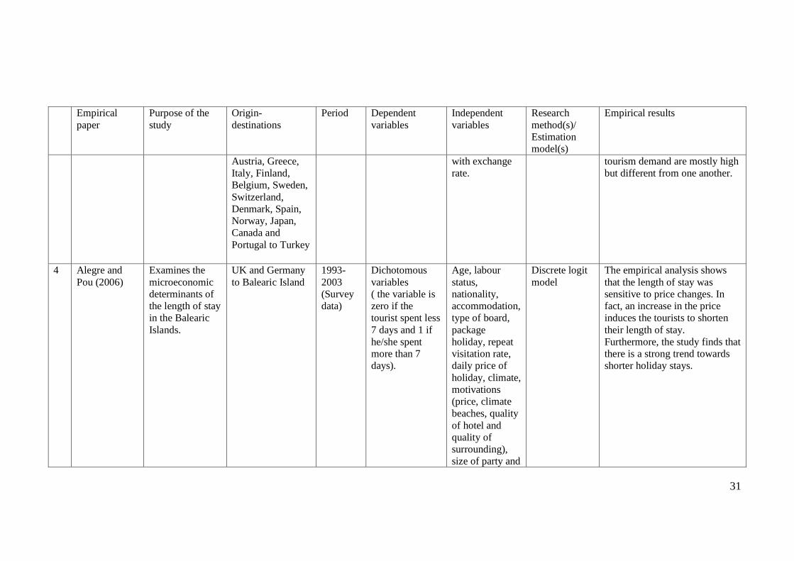
31
Empirical
paper Purpose of the
study Origin-
destinations
Period Dependent
variables Independent
variables Research
method(s)/
Estimation
model(s)
Empirical results
Austria, Greece,
Italy, Finland,
Belgium, Sweden,
Switzerland,
Denmark, Spain,
Norway, Japan,
Canada and
Portugal to Turkey
with exchange
rate. tourism demand are mostly high
but different from one another.
4 Alegre and
Pou (2006) Examines the
microeconomic
determinants of
the length of stay
in the Balearic
Islands.
UK and Germany
to Balearic Island 1993-
2003
(Survey
data)
Dichotomous
variables ( the variable is
zero if the
tourist spent less
7 days and 1 if
he/she spent
more than 7
days).
Age, labour
status,
nationality,
accommodation,
type of board,
package
holiday, repeat
visitation rate,
daily price of
holiday, climate,
motivations
(price, climate
beaches, quality
of hotel and
quality of
surrounding),
size of party and
Discrete logit
model The empirical analysis shows
that the length of stay was
sensitive to price changes. In
fact, an increase in the price
induces the tourists to shorten
their length of stay.
Furthermore, the study finds that
there is a strong trend towards
shorter holiday stays.
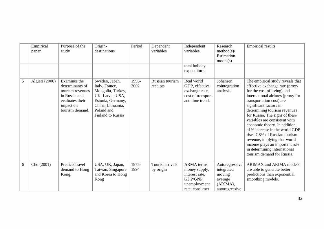
32
Empirical
paper Purpose of the
study Origin-
destinations
Period Dependent
variables Independent
variables Research
method(s)/
Estimation
model(s)
Empirical results
total holiday
expenditure.
5 Algieri (2006) Examines the
determinants of
tourism revenues
in Russia and
evaluates their
impact on
tourism demand.
Sweden, Japan,
Italy, France,
Mongolia, Turkey,
UK, Latvia, USA,
Estonia, Germany,
China, Lithuania,
Poland and
Finland to Russia
1993-
2002 Russian tourism
receipts Real world
GDP, effective
exchange rate,
cost of transport
and time trend.
Johansen
cointegration
analysis
The empirical study reveals that
effective exchange rate (proxy
for the cost of living) and
international airfares (proxy for
transportation cost) are
significant factors in
determining tourism revenues
for Russia. The signs of these
variables are consistent with
economic theory. In addition,
a1% increase in the world GDP
rises 7.8% of Russian tourism
revenue, implying that world
income plays an important role
in determining international
tourism demand for Russia.
6 Cho (2001) Predicts travel
demand to Hong
Kong.
USA, UK, Japan,
Taiwan, Singapore
and Korea to Hong
Kong
1975-
1994
Tourist arrivals
by origin ARMA terms,
money supply,
interest rate,
GDP/GNP,
unemployment
rate, consumer
Autoregressive
integrated
moving
average
(ARIMA),
autoregressive
ARIMAX and ARIMA models
are able to generate better
predictions than exponential
smoothing models.

33
Empirical
paper Purpose of the
study Origin-
destinations
Period Dependent
variables Independent
variables Research
method(s)/
Estimation
model(s)
Empirical results
price index, and
imports and
exports of the
tourist‟s country
integrated
moving
average with
explanatory
variables
(ARIMAX),
and
exponential
smoothing
models
7 Choi (2003) Examines the
leading
indicators of
hotel industry
growth in USA.
USA (Destination) 1966-
1993 Hotel industry
growth (HIG)
cycle in USA
America stock
exchange index,
number of
business
failures, CPI for
motor fuels,
hotel dividends
per share, GDP
of service, hotel
stock index,
money supply
(M2), New
York stock
exchange index,
Calculate HIG
using yearly
growth rate of
total hotel
revenue
receipts and
determine the
leading
indicators
using cross-
correlation
function.
The leading economic indicators
lead the peaks of the hotel
growth cycle by one-year-ahead,
with 67% accuracy. However,
during the troughs, the
indicators lead the hotel growth
by one-year-ahead, with 17%
accuracy.

34
Empirical
paper Purpose of the
study Origin-
destinations
Period Dependent
variables Independent
variables Research
method(s)/
Estimation
model(s)
Empirical results
prime interest
rate charged by
banks, S&P 500
stock price
index, savings
percentage of
disposable
income, and
wages.
8 Croes and
Vanegas Sr
(2005)
Models tourist
arrivals to
Aruba.
USA, the
Netherlands and
Venezuela to
Aruba
1975-
2000 Tourist arrivals
by origin Real GDP for
USA and the
Netherlands,
real per capita
GDP for
Venezuela, real
exchange rate,
lagged
dependent
variable,
dummy
variables (US
recession in
1979-1982,
1986 airlift
problems in
OLS and OLS
with
Cochrane-
Orcutt
approach
Income variable is the most
important determinant for all
origin countries. The income
elasticities range from 1.43 to
2.52, indicating that Aruba
tourism is a luxury product. For
tourism prices, real exchange
rates and relative prices are
found statistically significant,
but the elasticities are low for all
countries.

35
Empirical
paper Purpose of the
study Origin-
destinations
Period Dependent
variables Independent
variables Research
method(s)/
Estimation
model(s)
Empirical results
Aruba, political
instability in
1992,
Venezuela
devaluation and
social problems
in 1983, 1988
enhancement of
Air Aruba in
airlift between
Aruba and the
Netherlands,
and 1988 KLM
enhanced airlift
between the
Netherlands and
Aruba).
9 Daniel and
Ramos (2002) Models
international
tourist arrivals to
Portugal.
France, Germany,
the Netherlands,
Spain and UK to
Portugal
1975-
1997 Tourist arrivals
by origin Real GDP per
capita, relative
price, cost of air
travel, average
consumption of
a passenger car
and cost of
surface travel.
Johansen‟s
cointegration
analysis and
error
correction
model
Income and price variables are
important factors for the
demand. Furthermore, the
surface costs influence German
and French tourists in Portugal.
For the Netherlands and UK
tourists, the air flight cost
variable is an important factor.
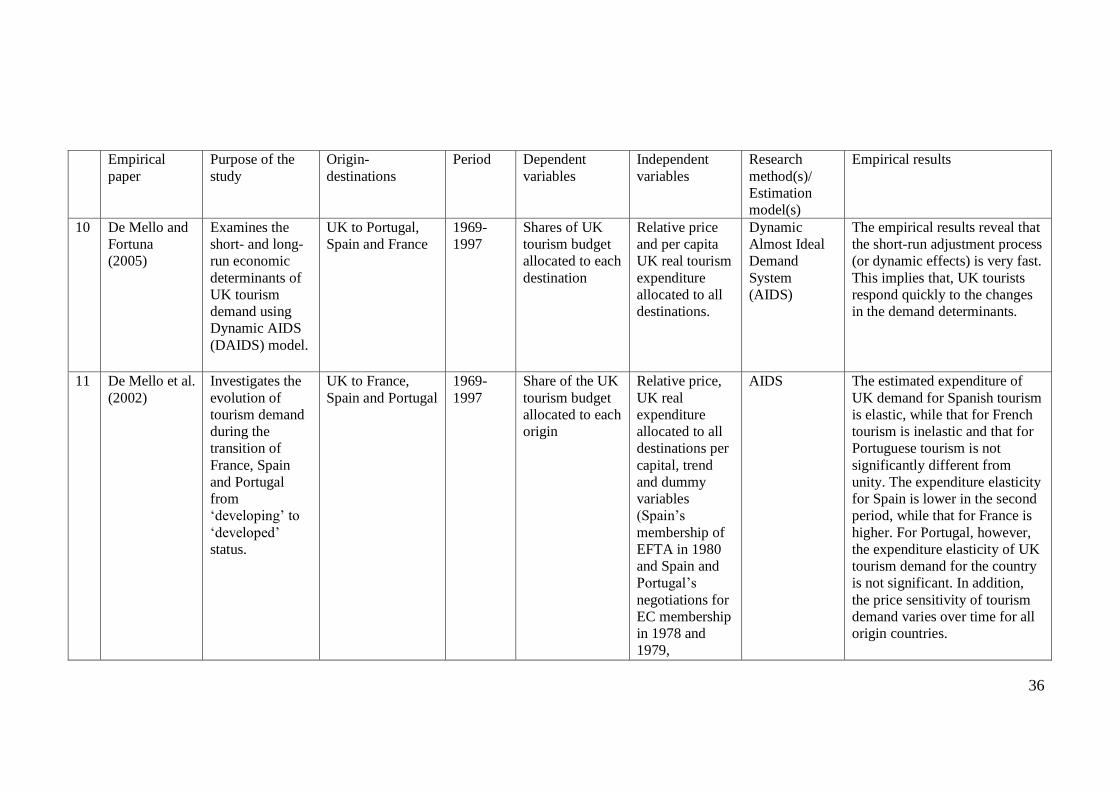
36
Empirical
paper Purpose of the
study Origin-
destinations
Period Dependent
variables Independent
variables Research
method(s)/
Estimation
model(s)
Empirical results
10 De Mello and
Fortuna
(2005)
Examines the
short- and long-
run economic
determinants of
UK tourism
demand using
Dynamic AIDS
(DAIDS) model.
UK to Portugal,
Spain and France 1969-
1997 Shares of UK
tourism budget
allocated to each
destination
Relative price
and per capita
UK real tourism
expenditure
allocated to all
destinations.
Dynamic
Almost Ideal
Demand
System
(AIDS)
The empirical results reveal that
the short-run adjustment process
(or dynamic effects) is very fast.
This implies that, UK tourists
respond quickly to the changes
in the demand determinants.
11 De Mello et al.
(2002) Investigates the
evolution of
tourism demand
during the
transition of
France, Spain
and Portugal
from
„developing‟ to
„developed‟
status.
UK to France,
Spain and Portugal 1969-
1997 Share of the UK
tourism budget
allocated to each
origin
Relative price,
UK real
expenditure
allocated to all
destinations per
capital, trend
and dummy
variables
(Spain‟s
membership of
EFTA in 1980
and Spain and
Portugal‟s
negotiations for
EC membership
in 1978 and
1979,
AIDS The estimated expenditure of
UK demand for Spanish tourism
is elastic, while that for French
tourism is inelastic and that for
Portuguese tourism is not
significantly different from
unity. The expenditure elasticity
for Spain is lower in the second
period, while that for France is
higher. For Portugal, however,
the expenditure elasticity of UK
tourism demand for the country
is not significant. In addition,
the price sensitivity of tourism
demand varies over time for all
origin countries.
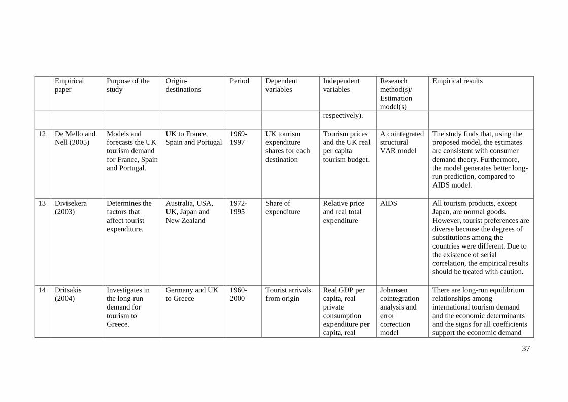
37
Empirical
paper Purpose of the
study Origin-
destinations
Period Dependent
variables Independent
variables Research
method(s)/
Estimation
model(s)
Empirical results
respectively).
12 De Mello and
Nell (2005) Models and
forecasts the UK
tourism demand
for France, Spain
and Portugal.
UK to France,
Spain and Portugal 1969-
1997 UK tourism
expenditure
shares for each
destination
Tourism prices
and the UK real
per capita
tourism budget.
A cointegrated
structural
VAR model
The study finds that, using the
proposed model, the estimates
are consistent with consumer
demand theory. Furthermore,
the model generates better long-
run prediction, compared to
AIDS model.
13 Divisekera
(2003) Determines the
factors that
affect tourist
expenditure.
Australia, USA,
UK, Japan and
New Zealand
1972-
1995 Share of
expenditure Relative price
and real total
expenditure
AIDS All tourism products, except
Japan, are normal goods.
However, tourist preferences are
diverse because the degrees of
substitutions among the
countries were different. Due to
the existence of serial
correlation, the empirical results
should be treated with caution.
14 Dritsakis
(2004) Investigates in
the long-run
demand for
tourism to
Greece.
Germany and UK
to Greece 1960-
2000
Tourist arrivals
from origin Real GDP per
capita, real
private
consumption
expenditure per
capita, real
Johansen
cointegration
analysis and
error
correction
model
There are long-run equilibrium
relationships among
international tourism demand
and the economic determinants
and the signs for all coefficients
support the economic demand

38
Empirical
paper Purpose of the
study Origin-
destinations
Period Dependent
variables Independent
variables Research
method(s)/
Estimation
model(s)
Empirical results
private
expenditure on
consumption
services per
capita, relative
prices,
transportation
cost and real
exchange rates.
theory.
15 Dritsakis and
Athanasiadis
(2000)
Focus on the
primary
influence of
social and
economic
changes on the
demand for
Greece tourism.
Austria, Benelux,
France, Germany,
Denmark, Italy,
UK, Holland,
Sweden, Finland,
Yugoslavia,
Switzerland,
Norway, USA and
Japan to Greece
1960 –
1993
Tourist arrivals
to Greece per
capita
Disposable
income per
capita, average
travel costs in
Greece, average
travel costs in
other competing
Mediterranean
countries,
exchange rate,
gross
investment in
fixed assets,
advertising
expenditures,
dummy
Univariate
log-linear
model
Income variable was not an
important economic
determinant, which contradicted
to previous literature.
Furthermore, average travel cost
in Greece was found to be
statistically not significant.
However, the average travel cost
in other competing destinations,
gross investment and the effects
of political stability appeared to
be crucial determinants for the
demand for Greece‟s tourism.

39
Empirical
paper Purpose of the
study Origin-
destinations
Period Dependent
variables Independent
variables Research
method(s)/
Estimation
model(s)
Empirical results
variables for
political
stability in
Greece, and
time trend.
16 Durbarry and
Sinclair
(2003)
Estimates the
magnitudes and
determinants of
French tourist
arrivals to
European
countries
France to Italy,
Spain and UK 1968-
1999 The share of
French tourism
budget in each
destination
Relative price,
real tourist
expenditure per
capita and
dummy
variables for the
world recession
in 1979 and
Gulf war in
1984.
AIDS Own prices are the main
demand determinants of the
French tourism market in
Europe. Own price elasticities
are high, ranging from -1.7 to -
2.2 for Italy, Spain and UK
tourism.
17 Eilat and
Einav (2004) To understand
the determinants
of international
tourism in the
world.
All regions in the
world 1985-
1998 Tourist arrivals
by origin-
destination
Tourism
receipts (% of
GNP) in origin
and destination,
relative price,
risk index in
destination,
trade in origin-
destination,
Pooled logit
regression International tourism demand to
developed countries is sensitive
to price movement, but was not
sensitive for the cases of
developing countries. Other
factors namely destination risk,
common border, common
language and distance are
important in determining

40
Empirical
paper Purpose of the
study Origin-
destinations
Period Dependent
variables Independent
variables Research
method(s)/
Estimation
model(s)
Empirical results
distance
between origin
and destination,
dummy
variables (same
language
regions and
common border)
tourism flows to both developed
and developing countries.
18 Eugenio-
Martin et al.
(2005)
Determines
whether Food-
and-Mouth
disease and 9/11
terrorist crisis
have significant
impacts on
different types of
tourists.
USA, France and
Germany to
Scotland
1979-
2003 Tourist arrivals
and tourism
receipts by
origin
GDP, real
exchange rate
between
Scotland and
origins, real
exchange rate
between
Scotland and
competing
destinations,
lagged
dependent
variable, and
trend, seasonal
and error
components.
Structural time
series model Tourists from different countries
respond differently to various
types of crises. Food-and-mouth
disease affected French tourists,
while the 9/11 terrorist attack
affected German tourists. For
US tourists, the arrivals declined
during the occurrence of both
crises, as well as the tourism
receipts were hardly affected.

41
Empirical
paper Purpose of the
study Origin-
destinations
Period Dependent
variables Independent
variables Research
method(s)/
Estimation
model(s)
Empirical results
19 Gallet and
Braun (2001)` Models US
tourist arrivals to
European
countries.
USA to UK,
France, Germany,
Italy, Switzerland,
Spain, Austria and
Denmark
1960-
1985 Number of visits
of US residents
to each
destination
Relative price
between USA
and destination,
US personal
disposable
income, price of
tourism in
competing
destinations and
lagged
dependent
variable.
Gradual
switching
regression
The income elasticities for most
European countries, except
Switzerland, increased between
1973 (the pre-adjustment
period) and 1976 (the post-
adjustment period), indicating
that growing numbers of US
residents consider travelling to
Europe as a luxury product. For
relative price variable, there
were mixed results. Price
elasticities for UK, Germany
and Italy decrease significantly
between the pre- and post-
adjustment periods, but the price
elasticities increase for
Switzerland. The cross-price
elasticities for most countries
are either negative in the pre-
adjustment period or become
negative in the post-adjustment
period.
20 Garcia-Ferrer
and Queralt
(1997)
Investigates the
forecast accuracy
of econometric
Spain 1983-
1991 Tourism receipts
and number of
tourists
Weighted
average of
industrial
Structural
model with
explanatory
The empirical results show that
econometric model (STSM)
produced the least forecast

42
Empirical
paper Purpose of the
study Origin-
destinations
Period Dependent
variables Independent
variables Research
method(s)/
Estimation
model(s)
Empirical results
model. production
index, relative
price to client
and competitor
countries,
stochastic trend
and seasonal
components,
and dummy
variables (Easter
and an outlier
exists in
November
1989).
variables
(STSM), basic
structural
model (BSM)
and ARIMA
accuracy.
21 Garin-Munoz
(2007) Examines the
economic
determinants of
German demand
for Spanish
tourism.
German to Spain 1991-
2003 Number of
overnight stays
in
accommodation,
and number of
German
travellers
GDP of
Germany per
capita, relative
price, cost of
crude oil,
dummy
variables
(changes in the
data source in
1999, the US
terrorist attack
GMM-
procedure of
Arellano and
Bond (1991)
[Dynamic
panel data
model]
The income variable shows
positive and significant. The
income elasticities of demand
are ranging from 2.07 to 4.47.
German tourists are sensitive to
prices and costs of travel. The
coefficients for dummy
variables are statistically
significant. The estimation of
the lagged dependent variable
shows statistically significant,

43
Empirical
paper Purpose of the
study Origin-
destinations
Period Dependent
variables Independent
variables Research
method(s)/
Estimation
model(s)
Empirical results
in 2001, and
effect of
environmental
tax levied in
2002) and
lagged
dependent
variable.
implying that tourism demand in
the previous period had an
important effect on current
tourism demand.
22 Garin-Munoz
(2006) Models
international
tourism demand
to Canary
Islands.
UK, Germany,
Holland, Sweden,
Ireland, Norway,
Denmark,
Belgium, Finland,
Italy, France,
Switzerland,
Austria, Poland
and Others to
Canary Islands.
1992-
2002 Tourist arrivals Lagged
dependent
variables, GDP,
relative prices,
price of crude
oil, and time
dummies.
Generalised
Method of
Moments
estimation of
dynamic panel
data regression
The lagged dependent variables
are found significant, indicating
that consumers‟ travel decisions
can be influenced by the word-
of-mouth. Also, income and
tourism prices have significant
influences on international
tourism demand for Canary
Islands.
23 Garin-Munoz
and Amaral
(2000)
Measures the
impact of the
economic
determinants of
the international
demand for
Germany, UK,
France, Italy,
Belgium,
Netherlands, USA,
Switzerland,
Sweden, Portugal,
1985-
1995 Number of
nights spent in
Spanish hotels
by origin
Gross National
Product (GNP),
exchange rate,
relative price
and dummy
variable for the
OLS and
Generalised
Least Square
(GSL) [panel
data analysis]
All economic variables are
significant. Income variable is
positive and elastic; the rest of
the variables are negative and
inelastic.

44
Empirical
paper Purpose of the
study Origin-
destinations
Period Dependent
variables Independent
variables Research
method(s)/
Estimation
model(s)
Empirical results
tourist services
in Spain.
Japan, Denmark,
Ireland, Norway,
Canada, Greece
and Mexico to
Spain
Gulf War in
1991
24 Gokovali et al.
(2007) Analyses the
determinants of
tourists‟ length
of stay at a
destination.
The Netherlands,
Germany, Britain
and Russia to
Turkey
2005 Average length
of stay Age, level of
education,
marital status,
household
income, type of
tourists, number
of past visits to
Turkey, quality
of services and
facilities, level
of hospitality,
attractiveness of
destination,
standard of
nightlife and
entertainment,
standard of
accommodation,
safely standard,
quality of sea
Cox and
Weibull
regressions
The variables that have positive
correlation with the length of
stay are nationality (for Russian
tourists), income, experience,
independent tour, timing of
reservation and familiarity. On
the other hand, the variables that
have negative correlation with
the length of stay are level of
education, level of daily
spending, number of annual
vacation plans, type of holiday,
nationality (for British tourists)
and type of accommodation.
Furthermore, variables such as
attractiveness of natural and
cultural environment, standard
of nightlife and entertainment,
and tourism promotion can
affect the length of stay.

45
Empirical
paper Purpose of the
study Origin-
destinations
Period Dependent
variables Independent
variables Research
method(s)/
Estimation
model(s)
Empirical results
and beaches,
distance, overall
attractiveness
and image of
Turkey,
promotional
effectiveness,
words of mouth
and number of
repeated visit.
25 Greenidge
(2001) Builds forecast
model using
structural time
series model for
the Barbados
tourism.
USA, UK, Canada
and Others to
Barbados
1968-
1997 Tourist arrivals
by origin Trend, seasonal
and cyclical
components,
GDP, relative
price between
origin and
Barbados and
relative price
between
Barbados and its
competing
destinations.
STSM, BSM,
and General
Structural
Model (GSM)
Using STSM models, the
coefficients for economic
variables have improved and
turned out to be correct. The
results also show that
seasonality appeared as an
important feature in the data.
26 Han et al.
(2006) Investigates US
demand for
USA to France,
Italy, UK and
1965-
1997 Share of US
expenditure in a
Relative price,
real per capital
AIDS The study finds that a price
increased in France, Italy and

46
Empirical
paper Purpose of the
study Origin-
destinations
Period Dependent
variables Independent
variables Research
method(s)/
Estimation
model(s)
Empirical results
tourism in
European
destinations.
Spain destination
country
(measured by
multiplying total
international
tourism receipts
of a destination
by the
proportion of
US tourist
quantity in the
destination to
the total US
tourist quantity
in all
destinations).
US tourism
expenditure
allocated in the
four destination
countries and a
dummy variable
for taking
account of the
effects of oil
price increased
in 1973-1976.
Spain would result in a
significant reduction in US
tourism demand, indicating that
maintaining price
competitiveness for these
countries is important. In
addition, when US tourists‟
budget rise, the market shares of
the UK and Spain decline while
the shares of France and Italy
increase. Finally, the choice of
price index has no significant
effects on the results obtained.
27 Hanly and
Wade (2007) Conducts
econometric
analysis of North
American tourist
expenditures in
Ireland.
North America,
USA and Canada
to Ireland
1985-
2004 Real
expenditure in
Ireland by the
North American
tourists
Real GDP, real
exchange rate,
number of
arrivals in the
under-18, 19-24,
35-44 and above
45 cohorts, and
dummy variable
for the 9/11
OLS and first-
differenced
log-linear
model
The US real exchange, the 25-
34 and over-45 age group are
found positive and significant in
influencing tourists‟
expenditures in Ireland. The
9/11 terrorist attacks on USA
had a positive and significant
impact on the North American
and US tourists‟ expenditures

47
Empirical
paper Purpose of the
study Origin-
destinations
Period Dependent
variables Independent
variables Research
method(s)/
Estimation
model(s)
Empirical results
terrorist attacks
on USA.
(except for tourists from
Canada), suggesting that
American tourists‟ marginal
propensity to spend (or
consume) has increased despite
the decline in the frequency of
travel due to the terrorist
attacks.
28 Hiemstra and
Wong (2002) Identifies the
major factors
affecting tourist
arrivals to Hong
Kong in the
1990s.
Japan, Mainland
China, Taiwan,
Thailand,
Australia, UK and
USA to Hong
Kong
1990-
1998 Tourist arrivals
by origin Lagged
dependent
variable,
personal
disposable
income in
origin, relative
price between
Hong Kong and
origin, price
index between
Hong Kong and
competing
destinations,
exchange rate,
cost of travel,
cost of travel to
Autoregressive
model GDP is the most important
variable for the Australia and
Mainland China data. Relative
prices and exchange rates
influence tourist arrivals to
Hong Kong. The change in
sovereignty of Hong Kong in
July 1997 affected most tourists
except Thai tourists.
Furthermore, seasonality exists
in the data series where the
Asian tourist arrivals tend to
peak in December whereas the
peak seasons for Western tourist
arrivals are March and October.

48
Empirical
paper Purpose of the
study Origin-
destinations
Period Dependent
variables Independent
variables Research
method(s)/
Estimation
model(s)
Empirical results
substitute
destinations,
short-term
interest rate,
average wage
rate for all
manufacturing
employees in
Hong Kong,
seasonal
dummies and
dummy
variables (the
effect of
currency
devaluation).
29 Hui and Yuen
(1998) Modelling the
demand of
Japanese tourist
arrivals to
British
Columbia.
Japan to British
Columbia 1980-
1992
The number of
Japanese tourists
arrivals to
British
Columbia
GDP per capita,
lagged
dependent
variable,
exchange rate,
seasonal dummy
variable and
relative prices
index.
OLS The empirical results show that
relative prices are insignificant
throughout the nine estimation
periods. Hence, the variable is
omitted. Income, seasonal dummies and
lagged dependent variables are
significant throughout the time.

49
Empirical
paper Purpose of the
study Origin-
destinations
Period Dependent
variables Independent
variables Research
method(s)/
Estimation
model(s)
Empirical results
However, exchange rates are
only significant for the time
periods of 1980-1988 and 1980-
1987. In terms of parameter stability,
all parameters vary over the nine
estimation period. As RMSE value is small, it
implied that the econometric
model predicts relatively well.
30 Hultkrantz and
Olsson (1997) Estimates the
impact of the
Chernobyl
nuclear accident
on domestic and
international
tourism in
Sweden.
Norway,
Denmark, Finland,
West Germany,
USA and other
countries to
Sweden
1978-
1989 Number of guest
nights ARMA
components and
intervention
variables
ARIMAX The Chernobyl nuclear accident
has no effects on domestic
tourism but have a persistent
negative effect on tourist
arrivals to Sweden.
31 Ismail et al.
(2000) Examines
monthly air
arrivals of
Japanese visitors
Japan to Guam 1987-
1997 Japanese
monthly air
arrivals to Guam
Monthly
seasonal
dummies,
monthly
OLS Income elasticity for Japanese
demand to Guam tourism is 1.7,
implying that Guam tourism is a
luxury product for Japanese. In

50
Empirical
paper Purpose of the
study Origin-
destinations
Period Dependent
variables Independent
variables Research
method(s)/
Estimation
model(s)
Empirical results
to Guam. Japanese
household
earnings and
dummy
variables for
natural
disasters, Asian
currency crisis
and lagged
dependent
variable.
terms of seasonality, January
has a high number of Japanese
tourists than in December.
Moreover, the dummy variables
are found statistically
insignificant.
32 Jensen (1998) Estimates
income and price
elasticities for
six most
important
tourists to
Denmark.
West Germany,
Sweden, Norway,
USA, UK and
Holland to
Denmark
1969-
1995 Number of
nights spent in
accommodation
Real private
consumption,
real GDP,
relative price
between
Denmark and
origin, real
exchange rate,
relative price
between
Denmark and its
competing
destinations,
trend and petrol
OLS All tourists visiting Denmark
are sensitive to changes in prices
and income. The estimates vary
considerably across different
types of tourists.

51
Empirical
paper Purpose of the
study Origin-
destinations
Period Dependent
variables Independent
variables Research
method(s)/
Estimation
model(s)
Empirical results
costs.
33 Jimenez
(2002) Analyses the
determinants of
the tourism
revenues and
residential
foreign
investment in
Spain.
Spain 1967-
1998 Tourism
revenues and
residential
foreign
investment.
Indicator of the
tourist services
competitiveness,
relative oil
price, GDP, real
interest
differential
(Spain-
Investment
countries),
communications
and transport
infrastructures
investment,
indicator of
competitiveness
in the real state
sector and
dummy
variables for the
Olympic Games
in 1992 and
abnormal year
to tourism and
Nonlinear
simultaneous
estimations
The long-run income and
tourism price elasticities for
tourism revenues are 2.67 and
-1.01, respectively. However,
the income variable is found to
be insignificant in the short-run.
Tourism revenues are less
sensitive to changes in the oil
price (the oil price elasticity was
-0.09). The short- and long-run
tourism revenues elasticities for
the residential foreign
investment are 2.37 and 0.84,
respectively. Moreover, the
residential foreign investment is
very sensitive to the indicator of
competitiveness in the real state
sector in the long run and
communication and
transportations infrastructure in
the short-run. Real interest
differential has a positive effect
to the residential foreign
investment.

52
Empirical
paper Purpose of the
study Origin-
destinations
Period Dependent
variables Independent
variables Research
method(s)/
Estimation
model(s)
Empirical results
investment in
1969.
34 Jones and Chu
Te (1995) Determines the
leading
indicators for
tourist arrivals to
Australia.
Australia
(Destination) 1974-
1993 Number of
short-term
overseas visitors
to Australia
OECD-GDP,
OECD-
unemployment,
CPI in
Australia,
outward
international air
fares, total
permanent
overseas arrivals
to Australia,
permanent
overseas
departures from
Australia, visa
issues in
Australia,
composite
leading
indicator trend
index (industrial
production),
OECD-total
Cross
correlation
function
Among the leading indicators,
this study finds that GDP,
unemployment and trade
weighted index of Australia‟s
currency exchange rate are the
main indicators that strongly
lead the turning points of the
visitor arrivals. In the late 1993,
the GDP in OECD countries has
declined while there was a rise
in unemployment rate. Hence,
these indicators suggest that
tourist arrivals to Australia
could be at a declining stage.
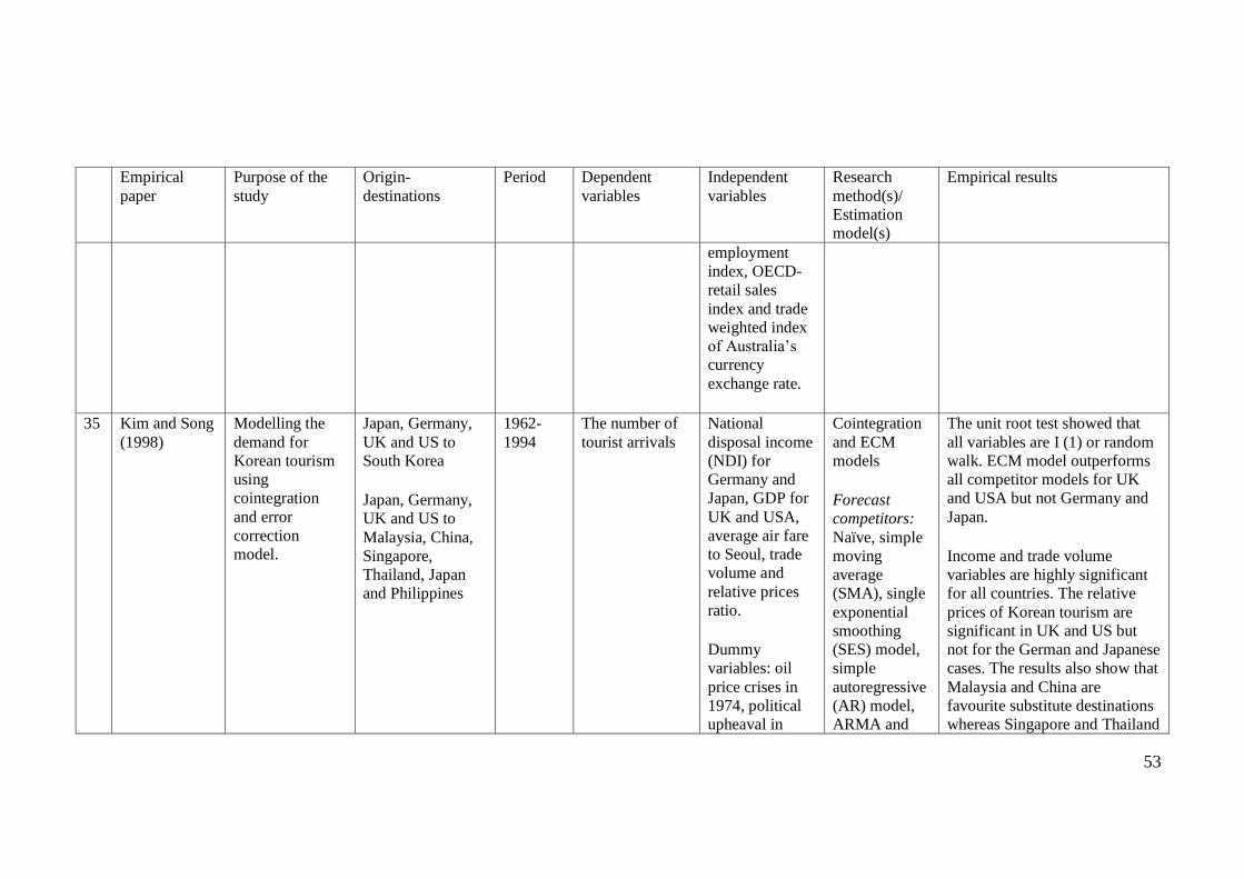
53
Empirical
paper Purpose of the
study Origin-
destinations
Period Dependent
variables Independent
variables Research
method(s)/
Estimation
model(s)
Empirical results
employment
index, OECD-
retail sales
index and trade
weighted index
of Australia‟s
currency
exchange rate.
35 Kim and Song
(1998)
Modelling the
demand for
Korean tourism
using
cointegration
and error
correction
model.
Japan, Germany,
UK and US to
South Korea Japan, Germany,
UK and US to
Malaysia, China,
Singapore,
Thailand, Japan
and Philippines
1962-
1994 The number of
tourist arrivals National
disposal income
(NDI) for
Germany and
Japan, GDP for
UK and USA,
average air fare
to Seoul, trade
volume and
relative prices
ratio. Dummy
variables: oil
price crises in
1974, political
upheaval in
Cointegration
and ECM
models Forecast
competitors:
Naïve, simple
moving
average
(SMA), single
exponential
smoothing
(SES) model,
simple
autoregressive
(AR) model,
ARMA and
The unit root test showed that
all variables are I (1) or random
walk. ECM model outperforms
all competitor models for UK
and USA but not Germany and
Japan. Income and trade volume
variables are highly significant
for all countries. The relative
prices of Korean tourism are
significant in UK and US but
not for the German and Japanese
cases. The results also show that
Malaysia and China are
favourite substitute destinations
whereas Singapore and Thailand

54
Empirical
paper Purpose of the
study Origin-
destinations
Period Dependent
variables Independent
variables Research
method(s)/
Estimation
model(s)
Empirical results
1980 and 1988
Seoul Olympics.
unrestricted
vector
autoregressive
(VAR) model.
are the complementary
destinations.
36 Kulendran and
Divisekara
(2007)
Quantifies the
effects of
marketing
expenditure on
international
tourist arrivals.
Japan, USA, UK
and New Zealand
to Australia
1980-
2001 Tourist arrivals
by origin Real GDP per
capita, relative
price between
Australia and
origin, relative
price between
Australia and
competing
destinations,
one-way
economic
airfare,
marketing
expenditure by
the Australian
Tourist
Commission
(ATC), dummy
variables for the
Sydney
Olympic Games
Johansen
cointegration
analysis and
ADLM
The coefficients for marketing
expenditure are not elastic and
the values of estimates are less
than the study has conducted in
previous studies. Furthermore,
the effects of „word-of mouth‟
and repeat visits are the
important factors in promoting
international visitor arrivals to
Australia. The cyclical pattern in
the origin‟s GDP significantly
influenced international tourist
arrivals to Australia. Moreover,
price elasticities for USA, Japan
and UK data are less than unity,
except for New Zealand tourism
demand.

55
Empirical
paper Purpose of the
study Origin-
destinations
Period Dependent
variables Independent
variables Research
method(s)/
Estimation
model(s)
Empirical results
and 9/11
terrorist attacks
in USA.
37 Kulendran and
King (1997) Forecasting
tourist arrivals to
Australia.
Japan, New
Zealand, UK-
Ireland and USA
to Australia
1975-
1994
The number of
tourist arrivals For Japanese
model: GNP,
relative price of
tourism for an
Australian
package tour
and package
tour to Hawaii. For New
Zealander
model:
production
based on real
GDP, relative
price between
Australia and
New Zealand,
and airflight
cost from
Auckland to
Sydney
ECM Forecasting
competitors:
Autoregressive
models (AR),
seasonal
ARIMA
models,
simple
regression
model with
ARMA errors
(RM) and
basic
structural
models with
intervention
explanatory
variable
(BSM)
In overall, AR model performs
well for longer lead times. In
terms of forecasting short lead
times, BSM performs well. For
ECM, the model forecasts
poorly in short lead time but
improved when the lead time
increased. For individual countries, RM
model forecasts best for the
USA data, while AR model is
best forecast model for the UK
data. For New Zealand, the
ARIMA model performs well in
short-term forecast and the AR
model is best for longer terms of
forecasts. For Japanese data,
there is no clear decision about
best forecast for short-term but
ECM performs well in the
longer term.

56
Empirical
paper Purpose of the
study Origin-
destinations
Period Dependent
variables Independent
variables Research
method(s)/
Estimation
model(s)
Empirical results
For British
model: GDP,
relative price
between
Australia and
Hawaii or
California, and
airflight cost
from London to
Sydney For USA model:
GNP, relative
price between
Australia and
Hawaii or
California, and
airflight cost
from San
Francisco to
Sydney Dummy
variables are:
(1) mid-1980s
where vigorous

57
Empirical
paper Purpose of the
study Origin-
destinations
Period Dependent
variables Independent
variables Research
method(s)/
Estimation
model(s)
Empirical results
advertisement
about Australia,
(2) 1987 for
Japanese
government
encourage
Japanese to
travel, (3)
World Expo in
1988, and (4)
1989 Australian
airline pilots‟
strike
38 Kulendran and
Wilson (2000) Identifies
economic
variables that
influence
business trips to
Australia.
USA, UK, New
Zealand and Japan
to Australia
1982-
1996 Number of
business tourists
to Australia by
origin
Real GDP,
openness to
trade, real
imports, relative
price and
number of
holiday trips.
Johansen
cointegration
analysis
Origin country income and
openness to trade are found to
be statistically significant.
Overall, the importance of the
economic variables differs from
country to country.
39 Kulendran and
Witt (2001) Investigates the
relative forecast
performance of
error correction
UK to France,
Germany, Greece,
Italy, Netherlands,
Portugal, Spain
1978-
1995 Number of UK
tourists in each
destination
UK real
personal
disposable
income per
Cointegration
analysis and
ECM
The results showed that ECM
outperforms least square
regression in forecasting but it
underperforms naïve models.

58
Empirical
paper Purpose of the
study Origin-
destinations
Period Dependent
variables Independent
variables Research
method(s)/
Estimation
model(s)
Empirical results
models (ECMs)
within the
context of
tourism demand.
and USA
capita, relative
price between
origin and UK,
relative price
between origin
and competing
destinations,
airfare between
origin and UK,
airfare between
competing
destination and
origin, dummy
variables (the
1979 oil crisis in
1979, bombing
of Libya in
1986, invasion
of Kuwait by
Iraq in 1990 and
Gulf War in
1991) and
lagged
dependent
variable.

59
Empirical
paper Purpose of the
study Origin-
destinations
Period Dependent
variables Independent
variables Research
method(s)/
Estimation
model(s)
Empirical results
40 Kulendran and
Witt (2003a) Examines the
forecasting
performance of
leading indicator
models.
UK to Germany,
Greece,
Netherlands,
Portugal, Spain
and the USA
1978-
1992 Number of UK
tourists in each
destination
Relative prices,
exchange rate,
real exchange
rate, personal
disposable
income and
GDP.
Leading
indicator
transfer
function (TF),
univariate
ARIMA and
error-
correction
(ECM) models
The TF model does not result in
an improvement in forecasting
performance.
41 Kulendran and
Witt (2003b) Determines the
best forecast
model for
business tourism
demand.
Japan, New
Zealand, UK and
USA to Australia
1982-
1998 Number of
business tourists Trend, seasonal
and irregular
components,
GDP in origin
and destination,
trade openness,
destination price
and number of
holiday tourist
visits.
STSM,
ARIMA,
ECM, BSM,
naïve and AR
models
Among the model, ARIMA and
BSM models outperform the
rest in forecasting. The study
also shows that STSM model do
not improve forecasting
performance. ECM generates
more accurate forecasts than
STSM model.
42 Lanza et al.
(2003) An econometric
analysis of
tourism
specialisation in
the long-run.
Austria, Belgium,
Denmark, France,
Germany, Greece,
Italy, Netherlands,
Portugal, UK,
1975-
1992 Budget share of
tourism in a
destination
Tourism price
and real total
expenditure
AIDS and
Johansen‟s
cointegration
analysis
The empirical results suggest
that tourism specialisation may
yield the real income growth
even if the potential productivity
growth in tourist activities is

60
Empirical
paper Purpose of the
study Origin-
destinations
Period Dependent
variables Independent
variables Research
method(s)/
Estimation
model(s)
Empirical results
Spain, Switzerland
and Turkey. poorer than in other sectors.
43 Ledesma-
Rodriguez et
al. (2001)
Estimates short-
and long-run
elasticities for
tourists visiting
the island of
Tenerife.
Germany, UK,
Spain, Sweden,
Norway, Finland,
the Netherlands,
Belgium, Austria,
France, Italy,
Denmark and
Switzerland to
Islands of Tenerife
1979-
1997 Tourist arrivals
by origin Lagged
dependent
variable, real
annual GDP of
each country,
relative price
per barrel of oil
between origin
and Tenerife,
exchange rate,
expenditure for
tourism
promotion and
capital stock in
infrastructure.
Static and
dynamic
models for
panel data
analysis
The income variable is highly
elastic, implying that travelling
to Tenerife is a luxury product.
Exchange rates and the costs of
trips are found statistically
significant but the latter is
inelastic. Infrastructure and
promotional expenditure are
also important determinants for
the demand.
44 Li et al. (2004) Assesses the
short- and long-
run demand
elasticities for
UK tourists in
Western Europe.
UK to Austria,
Belgium, Cyprus,
Denmark, Finland,
France, Germany,
Gibraltar, Greece,
Iceland, Irish
Republic, Italy,
1972-
2000 Per capita UK
tourist
expenditure
Relative prices
and real total
UK expenditure
TVP-LAIDS The study finds that TVP-
LAIDS model generates better
short- and long-term forecasts
than LAIDS and error correction
LAIDS (EC-LAIDS) models.

61
Empirical
paper Purpose of the
study Origin-
destinations
Period Dependent
variables Independent
variables Research
method(s)/
Estimation
model(s)
Empirical results
Luxembourg,
Malta, the
Netherlands,
Norway, Portugal,
Spain, Sweden,
Switzerland,
Turkey and former
Yugoslavia.
45 Li, Song and
Witt (2006) Assesses UK
tourism demand
for France,
Spain, Italy,
Greece and
Portugal
France, Spain,
Italy, Greece and
Portugal to UK
1972-
2004
Real tourism
spending per
capita
Household
disposable
income per
capita, relative
price and
substitute
prices, and
dummy
variables
(effects of the
oil crisis in
1974-75 and the
Gulf War in
1991).
Linear AIDS
(LAIDS) and
error
correction
AIDS (EC-
AIDS)
Changes in total UK tourist
expenditure have different
influences on tourism demand
for a destination. Demand for
tourism to Portugal and Greece
are strongly influenced by the
economic cycles in UK. UK
tourists are more sensitive to
price changes in the long-run
than in the short-run.
Furthermore, price changes in
Greece would highly affect UK
outbound tourism to Greece.
However, the price changes in
Italy have the least impact on
the UK tourists in the
destination. In terms of

62
Empirical
paper Purpose of the
study Origin-
destinations
Period Dependent
variables Independent
variables Research
method(s)/
Estimation
model(s)
Empirical results
destination substitution effects
for UK tourists, France is the
competing destination for Spain.
Finally, EC-AIDS generates
more accurate forecast than
LAIDS.
46 Li, Wong and
Witt (2006) Applies the time
varying
parameter linear
Almost Ideal
Demand System
(TVP-AIDS)
model in tourism
context.
UK to Austria,
Belgium, Cyprus,
Denmark, Finland,
France, Germany,
Gibraltar, Greece,
Iceland, Irish
Republic, Italy,
Luxembourg,
Malta,
Netherlands,
Norway, Portugal,
Spain, Sweden,
Swizerland,
Turkey and former
Yugoslavia
1972-
2000 Budget share of
travelling to a
destination
Relative price,
real total
expenditure
(total
expenditure
divided by
Stone price
index) and
dummy
variables (the
effects of oil
crises and Gulf
War)
TVP and
TVP-ECM Based on the estimation using
TVP model, the income
coefficients are positive and
statistically significant for all
destinations. The income
elasticities of UK tourism
demand range from 1.779 to
2.817. For the price variables,
the coefficients for relative price
are negative and significant for
all destinations, except Portugal.
Nevertheless, for substitute
price, the coefficients are
statistically significant for Italy
and Portugal, but the signs for
the coefficients are not
consistent with economic
theory.

63
Empirical
paper Purpose of the
study Origin-
destinations
Period Dependent
variables Independent
variables Research
method(s)/
Estimation
model(s)
Empirical results
In terms of forecasting accuracy
between TVP and TVP-ECM,
the latter model outperformed
the formal.
47 Lim (2004) Modelling
tourist arrivals
from Korea to
Australia.
Korea to Australia 1980-
1994 Tourist arrivals
from South
Korea
Real GNP
(proxy for
income
variable),
relative prices,
lagged
dependent
variables,
dummy
variables for
one-off events
(D89- removal
of travel
restrictions on
South Korea;
and D97-Asian
financial crisis)
and seasonal
dummy
variables.
Classical
linear
regression
All variables are statistical
significant, except dummy
variable for D89. The elasticities for the following
economic variables are: Income
(+5.95) and relative prices
(-6.10).

64
Empirical
paper Purpose of the
study Origin-
destinations
Period Dependent
variables Independent
variables Research
method(s)/
Estimation
model(s)
Empirical results
48 Lim et al.
(2008) Analyses the
impact of
changes in
income on
Japanese
outbound travel.
Japan to New
Zealand and
Taiwan
1980-
2004 Tourist arrivals
by origin Real GDP ARIMAX The income elasticities of
demand for New Zealand and
Taiwanese tourism range from
1.50 to 2.61. The study finds
that changes in income have
more significant impacts on
long-haul tourism demand (New
Zealand) than on short-haul
travel (Taiwan).
49 Lim and
McAleer
(2001)
Modelling long-
run economic
effects on tourist
arrivals from
Hong Kong and
Singapore to
Australia.
Hong Kong and
Singapore to
Australia
1975-
1996 Tourist arrivals
by source of
countries
Real GDP per
capita, real
private
consumption
expenditures per
capita, real
private
consumption
services per
capita, real
private
consumption
expenditures on
nondurables per
capita, real
round-trip
Johansen‟s
cointegration
and error-
correction
model
The elasticities of economic
variables for Hong Kong are:
real private consumption
services per capita (+2.26), real
round trip (return) coach
economy airfares in Fare
Construction Unit (-0.8) and real
exchange rate (-0.8). For
Singapore, real GDP per capita
(+1.59), real round trip (return)
coach economy airfares in Fare
Construction Unit (-2.29) and
exchange rate (-1.27). The remaining issue is that error
correction terms for Hong Kong

65
Empirical
paper Purpose of the
study Origin-
destinations
Period Dependent
variables Independent
variables Research
method(s)/
Estimation
model(s)
Empirical results
(return) coach
economy
airfares in Fare
Construction
Units, real
round-trip
(return) coach
economy
airfares in origin
currency,
exchange rate,
relative prices,
real exchange
rate and
seasonal dummy
variables.
and Singapore are not
significant. However, after the
author included seasonal
dummy variables and omitted
insignificant variables, the
results for Singapore have
improved but not for Hong
Kong.
50 Louca (2006) Examines
whether
expenditures on
the tourism
industry
contributed to
the growth of
tourism in
Cyprus.
Cyprus 1960-
2001 Three dependent
variables: (1)
Gross domestic
fixed capital
formation in
hotels and
restaurants, (2)
the
transportation
Tourist arrivals
and income
from the
tourism
industry.
Pairwise
Granger
causality test
and Johansen
cointegration
analysis
The results suggest that rises in
hotels and restaurants, and
advertising expenses increase
Cyprus‟s income and tourist
arrivals.

66
Empirical
paper Purpose of the
study Origin-
destinations
Period Dependent
variables Independent
variables Research
method(s)/
Estimation
model(s)
Empirical results
and
communication
expenses, (3)
advertisement
and promotional
expenses from
1975-2001
51 Luzzi and
Fluckiger
(2003)
Assesses the
demand for
tourism to
Switzerland, by
understanding
the reaction of
tourists to
economic
variables
according to
their origin.
USA, Japan, UK,
France, Italy,
Germany and
Spain to
Switzerland
1971-
1995 Number of
nights spent in
tourist
accommodations
by origin
GDP of origin,
relative price
between origin
and
Switzerland,
relative price
between
competing
destinations and
Switzerland,
dummy
variables (the
effect of oil
crisis in 1973
and 700th
anniversary of
the Federal Sate
in Switzerland
OLS This study finds that holidaying
in Switzerland is a luxury good
for America and Japan, due to
the long-distance of travel from
these two countries to
Switzerland. Unlike American
and European tourists, Japanese
tourists are relatively sensitive
to changes in relative price.
Furthermore, tourists from all
origin countries are sensitive to
the movement of exchange
rates.

67
Empirical
paper Purpose of the
study Origin-
destinations
Period Dependent
variables Independent
variables Research
method(s)/
Estimation
model(s)
Empirical results
in 1991), and
lagged
dependent
variable.
52 Lyssiotou
(2000) Investigates how
preference
endogeneity (or
habit
persistence)
affect short- and
long run tourism
expenditure
decisions.
UK to America
(USA and
Canada), France,
Italy, Greece,
Cyprus, Malta,
Spain, Portugal
and other North
European
countries
1979-
1991 British tourism
expenditure in
origin
Lagged
dependent
variable and
relative price.
Dynamic
demand
system model
Habit accounted for up to 36%
of current tourism expenditure.
There is a lag before the effect
of prices completely integrated
on UK tourists‟ budget. Tourist
decisions can be largely based
on experience gained from the
past visits.
53 Morley (1998) Modelling
dynamic
structure of
tourism demand
USA, Canada,
Germany, UK,
New Zealand,
Japan and
Malaysia to
Australia
1972-
1992 The number of
tourist arrivals
by purpose of
visit
Real GDP per
capita, economy
class air fare,
effective
exchange rate
between
Australia and
origin and
dummy
variables (i.e.
1988 for the
Presumably
OLS The results are as follows: (1)
income elasticities vary across
origins and within origins over
time (i.e. the elasticities are low
for both relatively low (e.g.
Malaysia) and high (e.g. UK)
income earners and high for
middle range income (e.g. Japan
and Germany). (2) The
elasticities vary when there were
changes in incomes, prices and

68
Empirical
paper Purpose of the
study Origin-
destinations
Period Dependent
variables Independent
variables Research
method(s)/
Estimation
model(s)
Empirical results
Australian
Bicentennial
and Expo, and
1989 for pilots‟
strike)
fares. This indicated that the
assumption of constant elasticity
is wrongly specified in previous
studies.
54 Narayan
(2006) Introduces the
convergence
hypothesis in
studying the
behaviour of
Australia‟s
tourism market.
USA, Canada,
India, Taiwan,
South Korea,
Japan, Hong
Kong, China,
Thailand,
Singapore, the
UK, Germany and
New Zealand to
Australia
1991-
2003 Tourist arrivals
from countries
of origin
Not specified. Panel unit root
regression Both univariate and panel unit
root tests results show the
hypothesis is rejected after
incorporating structural breaks.
This implied that convergence
of Australia‟s tourism markets
exists after including the
occurrence of unexpected
shocks into analysis.
55 Narayan
(2004) Models Fiji‟s
tourism demand
in the short-and
long-run.
Australia, New
Zealand and USA
to Fiji
1970-
2000 Tourist arrivals Per capita real
gross disposable
income, relative
hotel price
between Fiji and
origin, total cost
of holidaying in
Fiji relative to
Bali (destination
ARDL
approach to
cointegration
Growth in income in these
tourist source markets has a
positive impact on visitor
arrivals to Fiji while relative
hotel and substitute prices have
negative effects on visitor
arrivals.

69
Empirical
paper Purpose of the
study Origin-
destinations
Period Dependent
variables Independent
variables Research
method(s)/
Estimation
model(s)
Empirical results
substitute price),
real airfares and
dummy
variables (the
effects of coups
d‟etat).
56 Naude and
Saayman
(2005)
Investigates the
determinants of
tourist arrivals to
Africa.
America (Canada
and USA), Europe
and Africa regions
(domestic tourism)
to Africa
1996-
2000 Tourist arrivals
by total and
origin
Number of
internet users,
index of
political
stability,
number of frost
days on average
per year, air
distance,
number of
telephone lines
per employee,
prevalence of
malaria in 1994,
number of hotel
rooms available,
death rate, GDP
per capita, life
expectancy,
Generalized
least squares
(GLS) and
generalized
methods of
moments
(GMM) [Static
and dynamic
panel data
regression]
Demand for African tourism is
significantly affected by the
degree of political stability,
tourism infrastructure, internet
usage (proxy for marketing) and
urbanization rate (proxy for the
level of development in Africa).
All tourists are not sensitive to
tourism price, except Europe
tourists.

70
Empirical
paper Purpose of the
study Origin-
destinations
Period Dependent
variables Independent
variables Research
method(s)/
Estimation
model(s)
Empirical results
urbanization
rate, average
hotel room price
in 2002, and
adjusted CPI
(relative price).
57 Njegovan
(2005) Examines
whether leading
indicator
information can
generate accurate
prediction.
UK 1980-
2001 Binary indicator
variable for
growth or
decline in the
demand for
business travel
by air
Business
expectation
(Conference of
British Industry
(CBI) Change in
Optimism and
CBI Export
Optimism),
availability of
funds for
corporate travel
(gross operating
surplus of UK
corporations and
UK 3-month
yield treasury
bills), UK
economic
activity (UK
Probit model The results show that the
coefficients for all
macroeconomic leading
indicators influence the
direction of growth in business
air travel demand.

71
Empirical
paper Purpose of the
study Origin-
destinations
Period Dependent
variables Independent
variables Research
method(s)/
Estimation
model(s)
Empirical results
GDP, UK total
household final
consumption
and UK total
claimant count),
and world
economic
activity (US
GDP and US
composite
leading
indicator).
58 Nordstrom
(2005) Models the
demand for
Swedish tourism.
Germany and
Norway to
Sweden
1978-
1999 Number of guest
nights spent in
Swedish hotels
and cottages
Relative price
and gross
domestic
product (GDP),
autoregressive
(AR) and
stochastic
preference
components.
Multivariate
structural time
series model
Germans‟ and Norwegians‟
preferences evolved in exactly
in the same direction, implying
that these two countries have the
same preferences for visiting
Sweden. For German model, the
coefficients for the price and
income variables are not
significant. However, for
Norwegian tourists, they are
sensitive to the changes in prices
and their degree of habit
formation decrease over the

72
Empirical
paper Purpose of the
study Origin-
destinations
Period Dependent
variables Independent
variables Research
method(s)/
Estimation
model(s)
Empirical results
sample period.
59 Papatheodorou
(1999) Studies the
determinants of
tourists‟
expenditure in
the
Mediterranean
region.
West Germany,
France and UK to
Spain, Portugal,
Italy, Greece and
Turkey
1957-
1989 Percentage of
the aggregate
tourism
expenditure of
each origin in a
destination
Relative price,
real per capita
expenditure and
time trend
AIDS The expenditure and own-price
elasticities are found statistically
significant, but the value of
elasticities differed among the
origin-destination pairs.
60 Patsouratis et
al. (2005) Determines the
economic factors
that influence the
demand for
Greece tourism
and its
competing
destinations.
Great Britain,
Germany, France
and Italy to Greece
1980-
1997 Tourist arrivals
by origin National
disposable
income,
exchange rate,
CPI in Greece,
CPI in
alternative
destinations.
OLS Income variable is not
statistically significant.
Exchange rates are the most
important factor affecting
German tourists to Greece,
whereas the CPI of Greece
influences tourist arrivals from
Great Britain, France and Italy.
The empirical findings also
show that Spain is the main
competitor for Greece.
61 Payne and
Mervar (2002) Constructs an
econometric
model for
modelling
Croatia 1993-
1999 Tourism
revenues European Union
GDP, real
effective
exchange rate,
OLS All variables are statistically
significant in explaining real
tourism revenue for Croatia.
Particularly, the revenue is

73
Empirical
paper Purpose of the
study Origin-
destinations
Period Dependent
variables Independent
variables Research
method(s)/
Estimation
model(s)
Empirical results
tourism revenues
in Croatia. seasonal
dummies and
dummy variable
for military
action in 1995.
highly sensitively to the GDP of
European Union member
countries.
62 Qiu and Zhang
(1996) Examines the
determinants and
functional forms
of international
tourism demand
for travel to
Canada.
US, UK, France,
the former West
Germany and
Japan to Canada
1975-
1990 Tourist arrivals
and expenditure
by origin
Per capita GNP,
exchange rate,
travel price
index,
immigration,
crime rate, time
trend and
dummy
variables
(Summer
Olympics in
Montreal in
1976 and
Winter
Olympics in
Calgary in
1986).
OLS Determinants of tourism
demand vary by origin country.
Immigration variable has a
significant impact on tourists
from West Germany.
Furthermore, tourists from USA
and UK tend to spend more
during the 1986 Winter Olympic
event. Finally, most of the data
support linear functional form.
63 Qu and Lam
(1997) Modelling the
demand for
mainland
Mainland China to
Hong Kong 1984-
1995 The number of
Mainland
Chinese tourist
Level of
disposable
income per
OLS Of all the variables, only income
and relaxation of visa
requirement variables are

74
Empirical
paper Purpose of the
study Origin-
destinations
Period Dependent
variables Independent
variables Research
method(s)/
Estimation
model(s)
Empirical results
Chinese tourists
to Hong Kong. arrivals in Hong
Kong capita in China,
relative prices (a
ratio between
CPI in Hong
Kong and CPI
in China),
exchange rate
and dummy
variables
statistically significant.
64 Ouerfelli
(2008) Identifies the
factors
influencing the
destination
choice process
for Tunisia.
German, France,
Italy and UK to
Tunisia
1981-
2004 Tourist arrivals
by origin GDP per capita,
accommodation
capacity,
relative price
between Tunisia
and the origin,
and relative
price between
Tunisia and its
competing
destinations.
Cointegration
and ECM
The behaviour of European
tourists varies from one country
to another. The income and
price elasticities show that
tourism in Tunisia is regarded as
a luxury destination for French
and Italian tourists, but it is a
necessity destination for
German and UK tourists. Supply
factor is a significant variable
that could influence the tourists‟
choice of destination.
65 Riddington
(2002) Constructs a
forecast model
for the ski
UK to Geneva,
Salzburg, Lyon,
Lucerne,
1973-
2000 Number of
skiers Change in
Broad Money
and time trend
TVP The study finds that learning
curve approach can generate
better forecast than TVP model.

75
Empirical
paper Purpose of the
study Origin-
destinations
Period Dependent
variables Independent
variables Research
method(s)/
Estimation
model(s)
Empirical results
tourism in
Europe, using
learning curve
approach or
econometric
model.
Toulouse, Milan,
Munich, Verona
and Chambery.
66 Riddington
(1999) Assesses the
underlying
factors of
declining the
demand for ski
in Europe.
UK to Geneva,
Salzburg, Lyon,
Lucerne,
Toulouse, Milan,
Munich, Verona
and Chambery
1973-
1996
Number of
skiers Broad money
(M4) and time
trend
TVP The demand for ski in each
destination has experienced the
growth, decline and stable
stages. Furthermore, the
economic environment in UK
has a significant impact on the
skiing market.
67 Romilly et al.
(1998) Determines the
factors
influencing
tourism
spending.
138 countries
except Hong Kong
and Brunei
1989-
1995 Real per capita
international
tourism
spending by
country
Real per capita
GDP, real
exchange rate,
real exchange
rate volatility,
age, gender,
average
household size,
adult literacy
rate and
proportion of
Poolability
OLS panel
data regression
The strongest influence on
international tourist spending is
income, followed by real
exchange rate, age and degree of
urbanization.

76
Empirical
paper Purpose of the
study Origin-
destinations
Period Dependent
variables Independent
variables Research
method(s)/
Estimation
model(s)
Empirical results
urban
population
68 Rossello et al.
(2005) Models the
dynamic effects
of tourism
demand for
Balearic Islands.
UK and Germany
to Balearic Islands 1960-
2001 Tourist arrivals
by origin Income of
origin, relative
price, exchange
rate and dummy
variables
(miners‟ strike
in 1985 and the
Barcelona
Olympic Games
in 1992)
Dynamic
tourism
demand model
The income and price
coefficients vary across the
sample period. German income
and price elasticities converged
to zero but, for British, the
elasticities are stable over time.
69 Rossello-
Nadal (2001) Forecasts
European tourist
arrivals to
Balearic Islands
using leading
indicators.
UK and Germany
to Balearic Islands 1975-
1999 Monthly tourist
growth (MTG) Number of total
constructions,
CPI, foreign
trade/imports,
industrial
production,
relative prices
and exchange
rates.
General-to-
specific
analysis,
univariate
ARIMA and
naïve models
The leading indicators
significantly influence the
growth of tourist arrivals from
UK and Germany. Furthermore,
using leading indicator
methodology outperforms the
ARIMA and naïve models in
turning point forecasts.
70 Salman (2003) Estimates the
log-run
USA, UK,
Germany,
1980-
1998 Tourist arrivals
by origin Growth of
industrial output
Engle-Granger
approach of
The estimated long-run relative
price elasticity for Norway,

77
Empirical
paper Purpose of the
study Origin-
destinations
Period Dependent
variables Independent
variables Research
method(s)/
Estimation
model(s)
Empirical results
relationships
between monthly
tourist flows to
Sweden from
America, Europe
and Scandinavia
using
cointegration
analysis.
Denmark, Finland
and Norway to
Sweden
from origin,
monthly
personal income
for USA model,
relative price,
exchange rate,
lagged
dependent
variable,
Swedish
consumer price
index and
dummy
variables for
Chernobyl
accident in 1986
and Gulf war in
1991.
cointegration
analysis Denmark and Germany are -
1.15, -0.98 and -0.91,
respectively. Furthermore, the
income elasticities for UK and
Finland were 2 and 2.64.
However, the income elasticities
for Finland, Denmark and
Norway are 0.86, 0.6 and
0.0028, respectively. For the
estimates of long-run Swedish
consumer price index, the
elasticities for Germany and UK
are 1.62 and -7.92. Moreover,
both Chernobyl nuclear accident
and Gulf war have no significant
effects on international tourism
demand.
71 Salman et al.
(2007) Determines the
long-term
international
demand for
tourism in
Sweden.
The USA, the UK,
Germany, Finland,
Norway and
Denmark to
Sweden
1980-
1998 Tourist arrivals
by origin CPI,
temperature in
Sweden,
average
disposable
income,
nominal
Engle-Granger
cointegration
analysis
The study finds that income,
exchange rate and CPI have
significant effects on the
international tourism demand.
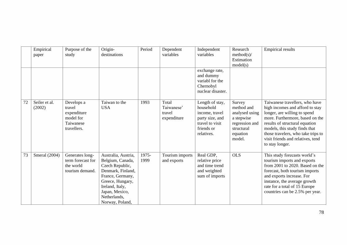
78
Empirical
paper Purpose of the
study Origin-
destinations
Period Dependent
variables Independent
variables Research
method(s)/
Estimation
model(s)
Empirical results
exchange rate,
and dummy
variabl for the
Chernobyl
nuclear disaster.
72 Seiler et al.
(2002) Develops a
travel
expenditure
model for
Taiwanese
travellers.
Taiwan to the
USA 1993 Total
Taiwanese‟
travel
expenditure
Length of stay,
household
income, travel
party size, and
travel to visit
friends or
relatives.
Survey
method and
analysed using
a stepwise
regression and
structural
equation
model.
Taiwanese travellers, who have
high incomes and afford to stay
longer, are willing to spend
more. Furthermore, based on the
results of structural equation
models, this study finds that
those travelers, who take trips to
visit friends and relatives, tend
to stay longer.
73 Smeral (2004) Generates long-
term forecast for
the world
tourism demand.
Australia, Austria,
Belgium, Canada,
Czech Republic,
Denmark, Finland,
France, Germany,
Greece, Hungary,
Ireland, Italy,
Japan, Mexico,
Netherlands,
Norway, Poland,
1975-
1999 Tourism imports
and exports Real GDP,
relative price
and time trend
and weighted
sum of imports
OLS This study forecasts world‟s
tourism imports and exports
from 2001 to 2020. Based on the
forecast, both tourism imports
and exports increase. For
instance, the average growth
rate for a total of 15 Europe
countries can be 2.5% per year.

79
Empirical
paper Purpose of the
study Origin-
destinations
Period Dependent
variables Independent
variables Research
method(s)/
Estimation
model(s)
Empirical results
Portugal, Slovenia,
Spain, Sweden,
Switzerland, UK
and USA.
74 Song and Witt
(2003) Develops a
model to forecast
tourist arrivals to
Korea.
Germany, Japan,
UK and USA to
Korea
1962-
1998 Tourist arrivals
by origin GDP in origin,
real trade
volume, relative
price between
origin and
Korea, price
index for
competing
destinations,
and dummy
variables
(World oil
crises in 1974,
political unrest
in 1980, Seoul
Olympics in
1988, the effect
of establishment
of the Tourism
Policy Council
in 1965 and
Autoregressive
distributive lag
model
(ADLM), and
ECM
For Germany and Japan, income
and price variables are not
significant. However, the prices
of tourism in substitute
destinations influence tourist
arrivals from German and Japan.
In addition, habit persistence or
words-of-mouth affects
Japanese demand for Korean
tourism. For UK and USA, all
variables are important to
determine the demand from
these two countries. Changing
policy and oil crisis are also the
factors that affect tourist arrivals
to Korea. In terms of forecast
accuracy, none of the models
predicts well across all
investigated origin countries.
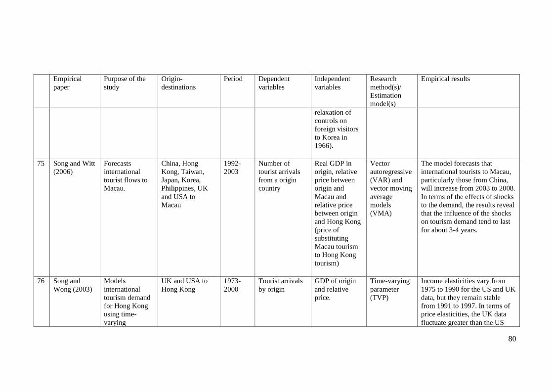
80
Empirical
paper Purpose of the
study Origin-
destinations
Period Dependent
variables Independent
variables Research
method(s)/
Estimation
model(s)
Empirical results
relaxation of
controls on
foreign visitors
to Korea in
1966).
75 Song and Witt
(2006) Forecasts
international
tourist flows to
Macau.
China, Hong
Kong, Taiwan,
Japan, Korea,
Philippines, UK
and USA to
Macau
1992-
2003 Number of
tourist arrivals
from a origin
country
Real GDP in
origin, relative
price between
origin and
Macau and
relative price
between origin
and Hong Kong
(price of
substituting
Macau tourism
to Hong Kong
tourism)
Vector
autoregressive
(VAR) and
vector moving
average
models
(VMA)
The model forecasts that
international tourists to Macau,
particularly those from China,
will increase from 2003 to 2008.
In terms of the effects of shocks
to the demand, the results reveal
that the influence of the shocks
on tourism demand tend to last
for about 3-4 years.
76 Song and
Wong (2003) Models
international
tourism demand
for Hong Kong
using time-
varying
UK and USA to
Hong Kong
1973-
2000
Tourist arrivals
by origin GDP of origin
and relative
price.
Time-varying
parameter
(TVP)
Income elasticities vary from
1975 to 1990 for the US and UK
data, but they remain stable
from 1991 to 1997. In terms of
price elasticities, the UK data
fluctuate greater than the US
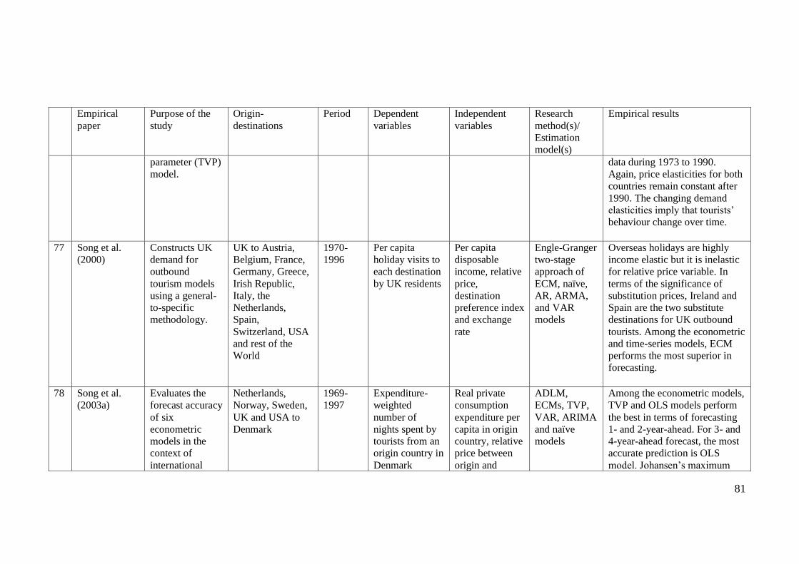
81
Empirical
paper Purpose of the
study Origin-
destinations
Period Dependent
variables Independent
variables Research
method(s)/
Estimation
model(s)
Empirical results
parameter (TVP)
model.
data during 1973 to 1990.
Again, price elasticities for both
countries remain constant after
1990. The changing demand
elasticities imply that tourists‟
behaviour change over time.
77 Song et al.
(2000) Constructs UK
demand for
outbound
tourism models
using a general-
to-specific
methodology.
UK to Austria,
Belgium, France,
Germany, Greece,
Irish Republic,
Italy, the
Netherlands,
Spain,
Switzerland, USA
and rest of the
World
1970-
1996 Per capita
holiday visits to
each destination
by UK residents
Per capita
disposable
income, relative
price,
destination
preference index
and exchange
rate
Engle-Granger
two-stage
approach of
ECM, naïve,
AR, ARMA,
and VAR
models
Overseas holidays are highly
income elastic but it is inelastic
for relative price variable. In
terms of the significance of
substitution prices, Ireland and
Spain are the two substitute
destinations for UK outbound
tourists. Among the econometric
and time-series models, ECM
performs the most superior in
forecasting.
78 Song et al.
(2003a) Evaluates the
forecast accuracy
of six
econometric
models in the
context of
international
Netherlands,
Norway, Sweden,
UK and USA to
Denmark
1969-
1997 Expenditure-
weighted
number of
nights spent by
tourists from an
origin country in
Denmark
Real private
consumption
expenditure per
capita in origin
country, relative
price between
origin and
ADLM,
ECMs, TVP,
VAR, ARIMA
and naïve
models
Among the econometric models,
TVP and OLS models perform
the best in terms of forecasting
1- and 2-year-ahead. For 3- and
4-year-ahead forecast, the most
accurate prediction is OLS
model. Johansen‟s maximum

82
Empirical
paper Purpose of the
study Origin-
destinations
Period Dependent
variables Independent
variables Research
method(s)/
Estimation
model(s)
Empirical results
tourism demand
to Denmark.
Denmark, price
index between
Denmark and
alternative
destinations,
travel cost, time
trend and
dummy
variables
(Effects of the
two oil crises in
1994 and 1979,
Gulf War in
1990, German
reunification in
1991, and
Chernobyl/USA
bombing of
Libya in 1986).
likelihood (JML)-ECM and
ARIMA are the worst forecast
models. Between JML-ECM
and Wickens-Breusch (WB)-
ECM, the latter model performs
well in all forecast periods.
79 Song et al.
(2003b) Examines the
demand for Thai
tourism.
Australia, Japan,
Korea, Malaysia,
Singapore, UK
and USA to
Thailand
1963-
2000
Tourist arrivals
by origin GPD in origin,
relative price
between origin
and Thailand,
price index for
competing
ADLM, ECM,
and ARIMA
models
Income is the main key factor
for the Australia, Korea and UK
data. Price variables are
important for the Australia,
Japan, Singapore and UK data.
Trade volume turns out to be

83
Empirical
paper Purpose of the
study Origin-
destinations
Period Dependent
variables Independent
variables Research
method(s)/
Estimation
model(s)
Empirical results
destinations,
treade volume,
and dummy
variables
(Effects of the
two oil crises in
1974 and 1979,
„Visit Thailand
Year‟ campaign
in 1987, the
Asian Financial
Crisis in 1997,
the Seoul
Olympics in
1988 and
student
demonstrations
in Korea in
1980).
significant in the cases of
Singapore and USA, which
could be due to high proportion
of business tourism from these
two countries. Regarding the
effects of one-off events, oil
crises affect tourist arrivals from
Japan, Korea and USA. For the
Asian financial crises, the
Koreans, Singaporeans tourists
as well as UK travellers are
affected the most. Among the
seven origin countries, the
number of tourists from Korea,
Malaysia and Japan are
forecasted as the largest tourism
generating countries, while the
highest growth rate of tourist
arrivals to Thailand is Korea.
80 Song et al.
(2003c) Identifis the
factors which
contribute to the
demand for
Hong Kong
tourism.
Australia, Canada,
China, France,
Germany,
Indonesia, India,
Japan, Korea,
Malaysia,
1973-
2000 Tourist arrivals Real GDP, CPI
for Hong Kong
and origin
countries,
substitute price
index, lagged
ADLM The most important factors that
determine the demand for Hong
Kong tourism are the costs of
tourism in Hong Kong,
economic condition (income) in
the origin, the costs of tourism

84
Empirical
paper Purpose of the
study Origin-
destinations
Period Dependent
variables Independent
variables Research
method(s)/
Estimation
model(s)
Empirical results
Philippines,
Singapore,
Taiwan, Thailand,
UK and USA to
Hong Kong.
dependent
variable and
dummy
variables for
one-off events
such as the 1974
oil crisis, and
1997 Asian
financial crisis.
in the competing destinations
and the word-of-mouth effect.
81 Tan and Wong
(2004) Examines the
existence of
structural change
in Hong Kong‟s
inbound tourism
demand after the
event of Asian
financial crisis in
1997.
Japan, South
Korea, Taiwan,
Indonesia,
Malaysia,
Philippines,
Singapore,
Thailand,
Australia, UK,
Germany, France,
Canada and USA
to Hong Kong
1980-
2000 Per capita real
tourism receipt
and tourist
arrivals by
origin
Real GDP per
capita, relative
price and
dummy variable
for Asian
financial crisis
in 1997.
Feasible
Generalized
Least Square
(FGLS) panel
data regression
Income appears as the most
important factor that affects the
tourism receipts and tourist
arrivals. After the crisis,
changes in relative price
variable have more impacts on
tourist arrivals than tourism
receipts.
82 Tan et al.
(2002a) Examines the
major factors
that influence the
tourist flows to
Australia,
Germany, Japan,
Singapore, UK
and USA to
1980-
1997 Tourist arrivals
by origin Relative price
between origin
and destination,
time trend,
OLS with
Cochrane-
Orcutt
iterative
Tourists from the same origin
country respond to changes in
income and prices differently,
depending upon the destination.

85
Empirical
paper Purpose of the
study Origin-
destinations
Period Dependent
variables Independent
variables Research
method(s)/
Estimation
model(s)
Empirical results
Indonesia and
Malaysia.
Malaysia and
Indonesia country dummy
variables and
special-event
dummies
(formation of
organization in
1989 for
Indonesia and
1987 for
Malaysia).
procedure Furthermore, not all income
variables in all origin-
destination country pairs are
found significant in this study.
Real exchange rates, dummy
variables and trend (proxy for
changing tastes) are important
factors for tourist arrivals to
Malaysia and Singapore.
83 Tan et al.
(2002b) Evaluates the
stability of
inbound tourism
demand models
for Indonesia
and Malaysia.
Japan, Singapore,
Australia, USA,
UK and Germany
to Indonesia and
Malaysia
1980-
1997 Tourist arrivals
by origin GDP in origin,
relative price
between origin
and destination,
exchange rate,
real exchange
rate, trend and
dummy
variables
(Persian Gulf
War in 1991,
Visit ASEAN
Year in 1992,
Asian currency
crises in 1997
Feasible
generalized
least square
panel data
regression
The demand elasticities are
different between pre- and post-
tourism formation periods. The
income elasticities are high
before the formation but they
gradually reduce after that. The
price elasticities are negative
and significant but the values
are less than one. The
coefficient for time-trend term is
significant, indicating that other
factors such as changes in tastes,
destination preferences and
demography influence the
demand for Malaysian and

86
Empirical
paper Purpose of the
study Origin-
destinations
Period Dependent
variables Independent
variables Research
method(s)/
Estimation
model(s)
Empirical results
and Visit
Malaysia Year
in 1990 and
1994).
Indonesian tourism.
84 Tse (2001) Investigates the
impact of
economic factors
on tourist
expenditure and
hotel room
occupancy rate
in Hong Kong.
Australia,
Belgium, Canada,
China, France,
Germany, Italy,
Japan, the
Netherlands,
Singapore, South
Korea,
Switzerland,
Taiwan, UK and
USA to Hong
Kong
1973-
1998 Real per capita
tourist spending
and hotel room
occupancy rate
Exchange rate,
length of stay,
tourist arrivals
and price.
Non-linear
least square Real tourism expenditure
strongly depends on expected
income, expected exchange rate
and price level. In addition, the
hotel occupancy rate is
influenced by tourist flows,
exchange rates, price level and
length of stay.
85 Turner and
Witt (2001a) Examines origin-
destination pairs,
which involve
longer travel
distances and
fewer direct
economic ties.
Australia, Japan,
UK and USA to
New Zealand
1978-
1997 Tourist arrivals
by purpose of
visit
Destination
living costs,
airfare, retail
sales, new car
registrations,
GDP, survey of
future
manufacturing,
Structural
equation
modelling
Trade openness, new private car
registrations, retail sales and
domestic loans are important
determinants of business
tourism demand. For holiday
tourism demand, retail sales,
GDP and new private car
registrations are important

87
Empirical
paper Purpose of the
study Origin-
destinations
Period Dependent
variables Independent
variables Research
method(s)/
Estimation
model(s)
Empirical results
survey of
consumer
confidence,
survey of
overall
prospects, trade
openness,
exports,
imports,
domestic loans,
number of
working days
lost and
population.
influences. In addition, tourists
who were visiting friends and
relatives (VFR) are strongly
influenced by new private car
registrations, retail sales,
destination price, airfare, GDP,
exports, imports and the survey
of consumer confidence are
important influences on VFR
tourist flows.
86 Turner and
Witt (2001b) Models tourism
demand using
structural time
series model.
USA, Australia,
Japan and UK to
New Zealand
1978-
1998 Tourist arrivals
by purpose of
visit
Trend, seasonal
and cyclical
components,
GDP, trade
openness and
airfare.
STSM, BSM
and naïve
models
STSM outperforms naïve model
but it underperforms BSM
model. In terms of the
significance of variables, the
study finds that income,
transport costs and trade
openness influence tourism
demand for New Zealand.
87 Turner et al.
(1998)
Examine a
simultaneous
UK to France,
Germany, Greece,
1978-
1995
Number of UK
tourists outflows
UK population,
UK real
Goodness-of-
fit index
Business tourism for all
destinations can be explained by

88
Empirical
paper Purpose of the
study Origin-
destinations
Period Dependent
variables Independent
variables Research
method(s)/
Estimation
model(s)
Empirical results
relationship
between
explanatory and
dependent
variables, and
also any
relationship
between
different
dependent
variables.
Italy, Netherlands,
Portugal and Spain
by purpose of
visits
personal
disposable
income per
capita, living
costs in
destination
relative to UK,
living costs in
destination
relative to
competing
foreign
destinations,
real airfare to
destination,
airfare to
destination
relative to
competing
foreign
destinations,
UK real GDP,
UK real imports
from
destination, UK
real exports to
destination,
(GFI),
adjusted
goodness of fit
index (AGFI),
root mean
square error of
approximation
(RMSEA)
economic variables. For the
determination of holiday tourist
flows, social variables such as
migration were more important
compared to economic
variables. For visiting friends
and relatives (VFR), economic
variables were more important
than social variables.
Furthermore, the importance of
explanatory variables for
different types of visiting
purposes varied across
countries.
In terms of the relationships
among dependent variables, this
study had found that there was a
relationship between holiday-
makers and VFR. This implied
that those tourists who were
visiting friends and relatives
tend to be a holiday-maker as
well.

89
Empirical
paper Purpose of the
study Origin-
destinations
Period Dependent
variables Independent
variables Research
method(s)/
Estimation
model(s)
Empirical results
migration into
UK from
destination,
migration out of
UK to
destination, UK
real retail sales,
survey of UK
business
confidence
88 Turner et al.
(1997) Modelling
tourism demand
using composite
national
indicators.
USA, Japan, UK
and New Zealand
to Australia
1975-
1996
The number of
tourist arrivals
by purpose of
visits
National income
(GNP or GDP),
unemployment
rate, forward
exchange rate,
money supply,
exports and
imports Intervention (or
dummy)
variables are:
(1) mid-1980s
where vigorous
advertisement
Seasonal
ARIMA and
transfer
function
models
The authors employ cross-
correlation to examine the
interrelationship between the
indicators and tourist arrivals.
They find that majority of the
indicators leads tourist arrivals.
This implies that the indicators
can provide a warning sign
about the direction of the tourist
arrivals. However, these
indicators are incorporated in
the transfer function model, not
all indicators show statistically
significant and the results varied
according to the country of
origin. Furthermore, leading

90
Empirical
paper Purpose of the
study Origin-
destinations
Period Dependent
variables Independent
variables Research
method(s)/
Estimation
model(s)
Empirical results
about Australia,
(2) 1987 for
Japanese
government
encourage
Japanese to
travel, (3)
World Expo in
1988, and (4)
1989 Australian
airline pilots‟
strike
indicators cannot predict
disaggregated data namely,
holiday-tourists and visiting
friends and relatives. In terms of forecasting accuracy,
there were mixed results. The
transfer function model only
outperformed ARIMA model
for some countries (i.e. New
Zealand) and disaggregated
business travel.
89 Turner et al.
(1998) Examines a
simultaneous
relationship
between
explanatory and
dependent
variables, and
also any
relationship
between
different
dependent
variables.
UK to France,
Germany, Greece,
Italy, Netherlands,
Portugal and Spain
1978-
1995 Number of UK
tourists outflows
by purpose of
visits
UK population,
UK real
personal
disposable
income per
capita, living
costs in
destination
relative to UK,
living costs in
destination
relative to
competing
Econometric
structural
equation
modelling
(LISREL) path
analysis
Business tourism for all
destinations can be explained by
economic variables. For the
determination of holiday tourist
flows, social variables such as
migration are more important
compared to economic
variables. For visiting friends
and relatives (VFR), economic
variables are more important
than social variables. Furthermore, the importance of

91
Empirical
paper Purpose of the
study Origin-
destinations
Period Dependent
variables Independent
variables Research
method(s)/
Estimation
model(s)
Empirical results
foreign
destinations,
real airfare to
destination,
airfare to
destination
relative to
competing
foreign
destinations,
UK real GDP,
UK real imports
from
destination, UK
real exports to
destination,
migration into
UK from
destination,
migration out of
UK to
destination, UK
real retail sales,
survey of UK
business
confidence
explanatory variables for
different types of visiting
purposes differs across
countries. In terms of the relationships
among dependent variables, this
study finds that there is a
relationship between holiday-
makers and VFR. This implies
that those tourists who are
visiting friends and relatives
tend to be a holiday-maker as
well.

92
Empirical
paper Purpose of the
study Origin-
destinations
Period Dependent
variables Independent
variables Research
method(s)/
Estimation
model(s)
Empirical results
90 Vanegas and
Croes (2000) Examines
international
tourism demand
to Aruba from
USA.
USA to Aruba 1975-
1996 Tourist arrivals
from USA Real GDP,
relative price,
real exchange
rate, lagged
dependant
variable and
dummy
variables (the
effect of US
recession from
1979 to 1981,
airlift problems
in Aruba in
1986 and Gulf
War in 1992)
OLS US tourists appear to be highly
sensitive to income variable.
The coefficients for relative
price variable are negative but
not significant. Furthermore, the
exchange rate variable is
positive and not significant.
91 Vogt (2008) Estimates real
income and
relative price
elasticities of
demand for US
exports and
imports of
tourism.
Destination: USA 1973-
2002 Quantity of
exports and
imports of
tourism demand
Price of tourism
in the US, world
price of tourism,
exchange rate,
world income,
and real income
of the US.
Granger-Engle
cointegration
procedure
US tourism exports are
relatively more sensitive to the
determinants of international
tourism than US tourism
imports.
92 Vogt and
Wittayakorn
Investigate the
effects of world
Thailand 1960 –
1993
Real tourism
expenditures in
Relative price
between
Univariate
log-linear
The study finds that the short-
and long-run relative price

93
Empirical
paper Purpose of the
study Origin-
destinations
Period Dependent
variables Independent
variables Research
method(s)/
Estimation
model(s)
Empirical results
(1998) income and the
relative price of
tourism in
Thailand on
Thailand‟s
exports of
tourism.
Thailand Thailand and
the World,
lagged relative
price, exchange
rates, lagged
exchange rates,
world income,
lagged world
income and
lagged
dependent
variable.
model coefficients show positive and
incorrect signs. Furthermore, the
short- and long-run income
elasticities of demand have
correct signs but neither of them
is statistically significant.
Moreover, the study reveals that
the value of the short-run
exchange rate elasticity exceeds
one but the elasticity drops to
less than unity in the long-run.
93 Wang (2008) Examines the
impact of crisis
events on the
demand for
Taiwanese
tourism.
Japan to Taiwan 1996-
2006 Tourist arrivals
from Japan Real GDP,
relative prices,
nominal
exchange rate,
international oil
price, and
dummy
variables (the
Asian financial
crisis,
earthquake in
Taiwan, 9/11
terrorist attacks
and SARS virus
ARDL Income and foreign exchange
rates are the important
explanatory variables for
Taiwanese tourism demand. For
the crises impacts, the study
finds that the Asian financial
crisis has lesser impacts on the
demand. However, the negative
impacts on Taiwanese tourism
were greater for the SARS
outbreak, 9/11 terrorist attacks,
and earthquake.
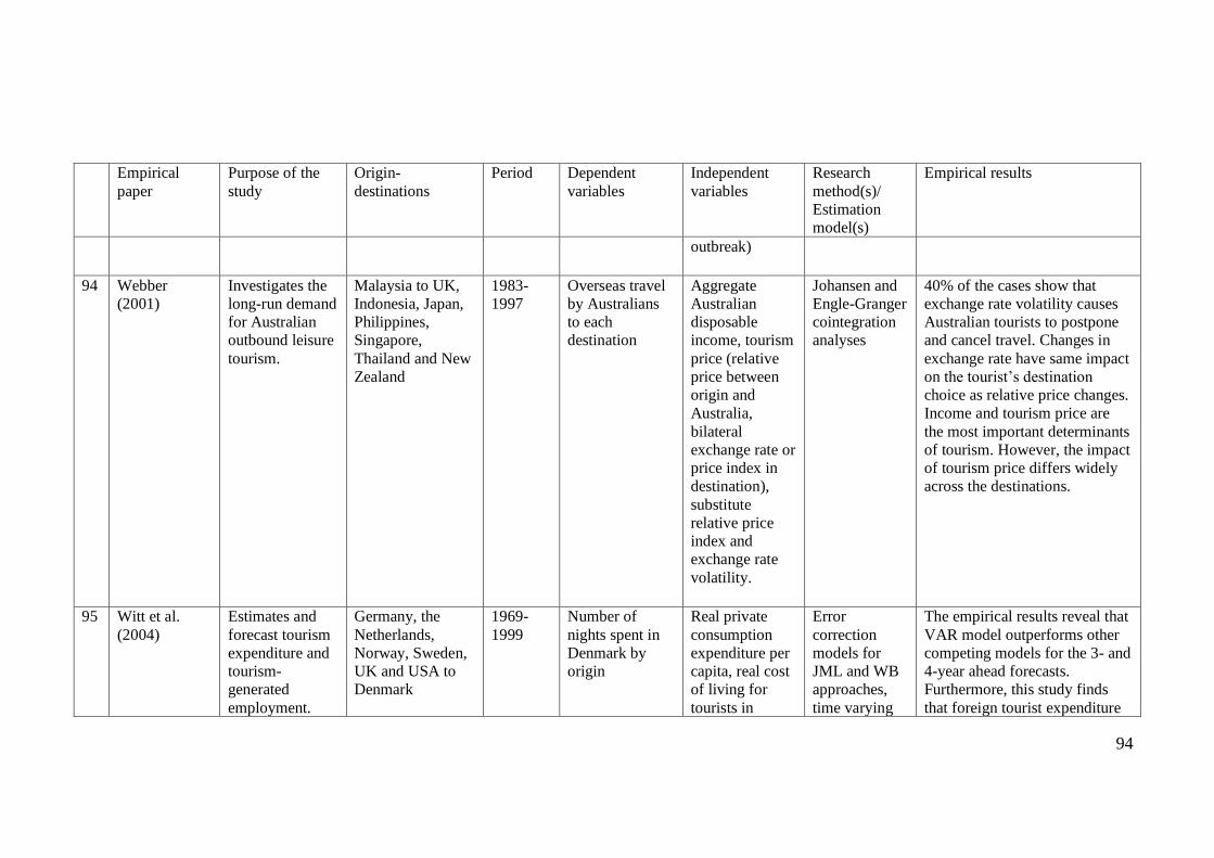
94
Empirical
paper Purpose of the
study Origin-
destinations
Period Dependent
variables Independent
variables Research
method(s)/
Estimation
model(s)
Empirical results
outbreak)
94 Webber
(2001) Investigates the
long-run demand
for Australian
outbound leisure
tourism.
Malaysia to UK,
Indonesia, Japan,
Philippines,
Singapore,
Thailand and New
Zealand
1983-
1997 Overseas travel
by Australians
to each
destination
Aggregate
Australian
disposable
income, tourism
price (relative
price between
origin and
Australia,
bilateral
exchange rate or
price index in
destination),
substitute
relative price
index and
exchange rate
volatility.
Johansen and
Engle-Granger
cointegration
analyses
40% of the cases show that
exchange rate volatility causes
Australian tourists to postpone
and cancel travel. Changes in
exchange rate have same impact
on the tourist‟s destination
choice as relative price changes.
Income and tourism price are
the most important determinants
of tourism. However, the impact
of tourism price differs widely
across the destinations.
95 Witt et al.
(2004) Estimates and
forecast tourism
expenditure and
tourism-
generated
employment.
Germany, the
Netherlands,
Norway, Sweden,
UK and USA to
Denmark
1969-
1999 Number of
nights spent in
Denmark by
origin
Real private
consumption
expenditure per
capita, real cost
of living for
tourists in
Error
correction
models for
JML and WB
approaches,
time varying
The empirical results reveal that
VAR model outperforms other
competing models for the 3- and
4-year ahead forecasts.
Furthermore, this study finds
that foreign tourist expenditure

95
Empirical
paper Purpose of the
study Origin-
destinations
Period Dependent
variables Independent
variables Research
method(s)/
Estimation
model(s)
Empirical results
Denmark,
tourism prices
in substitute
destinations,
time trend and
dummy
variables (oil
crises in 1975
and 1979, Gulf
War in 1991,
German
unification in
1991 and US
bombing in
Libya in 1986).
parameter,
ADLM, VAR,
ARIMA and
naïve models
have major impacts on
employment in the retail, hotel
and restaurant sectors in
Denmark.
96 Witt et al.
(2003) Assesses the
forecast accuracy
of various
econometric and
time-series
models in the
case of
international
tourism demand
to Denmark.
Germany,
Netherlands,
Norway, Sweden,
UK and USA to
Denmark
1969-
1997 The
expenditure-
weighted
number of
nights spent by
each tourist
origin in
Denmark
Lagged
dependent
variables, real
private
consumption
expenditure per
capita, relative
prices, price of
substitution,
time trend, and
Autoregressive
distributed lag
model
(ADLM),
ECM, TVP,
ARIMA and
naïve no-
change (or
random walk)
models.
The study finds that the TVP
model outperforms other
competing models for 1-year-
ahead forecasts. However, no
model significantly outperforms
the no-change model for 2- and
3-years-ahead forecasting
horizons.

96
Empirical
paper Purpose of the
study Origin-
destinations
Period Dependent
variables Independent
variables Research
method(s)/
Estimation
model(s)
Empirical results
dummy
variables for
two oil crises,
Germany
unification and
Chernobyl
disaster and US
bombing of
Libya.
97 Wong et al.
(2006)
Forecasts
international
tourist arrivals to
Hong Kong, and
determine the
best forecast
model for Hong
Kong‟s tourism
demand.
Australia, Canada,
France, Germany,
the UK and the
USA to Hong
Kong
1973-
2002 Tourist arrivals
by origin GDP, relative
prices, and
substitute
prices.
Bayesian
vector
autoregressive
(BVAR),
autoregressive
(AR) and
VAR models
The study finds that BVAR
model outperforms all other
competing models.
98 Zhang (1998) Modelling the
demand for
Hong Kong
tourism.
China, Taiwan,
Japan, USA, UK,
Canada, France
and Germany to
Hong Kong
1975-
1993 The number of
tourist arrivals Per capita GDP,
exchange rate
and number of
crimes divided
by population in
Hong Kong
OLS?? All estimated coefficients for
GDP are positive. Except for
USA, the variable is highly
significant for every other
country.

97
Empirical
paper Purpose of the
study Origin-
destinations
Period Dependent
variables Independent
variables Research
method(s)/
Estimation
model(s)
Empirical results
Exchange rate variable is highly
significant for all countries
except for Taiwan. While all
estimated coefficient of this
variable has the expected correct
sign, except for the Taiwan case. For crime rate, the coefficient is
negative for every country but it
is significant only for USA,
Canada and China.

98
Appendix 2.2. A summary of empirical research on domestic tourism demand Empirical
paper Purpose of study Tourism
destination
Period Main focused
group(s)/
independent
variable(s)
Factors/
independent
variables
Research
method(s)/
Estimation
model(s)
Empirical results
1 Alonso et al.
(2007) Investigates the
characteristics of
domestic winery
visitors in New
Zealand and
compare their
differences with
international
winery visitors.
New
Zealand 2003-
2004 Number of
domestic and
international
visitors in
New
Zealand‟s
vineyards.
Demographic
(income,
gender,
education level,
decision-maker
and planning,
and travel
budget), wine
knowledge and
consumption
(Wine
knowledge and
number of
bottles and
wine glasses
consumed), and
winery
experience
(Expenditure
and number of
purchases)
Survey
method The travel characteristics of
domestic winery visitors are
different from their counterparty
in terms of winery expenditures.
Domestic tourists spend more in
wine purchases than international
visitors.
2 Athanasopoul
os, G. and
Hyndman, R.
Aims to model and
forecast Australian
tourism demand.
Australia 1998-
2005
Domestic
visitor nights
by purpose of
Personal debts,
GDP per
capita, prices of
OLS and
Seemingly
Unrelated
The study shows that personal
debt has positive impact on
Australian domestic tourism

99
Empirical
paper Purpose of study Tourism
destination
Period Main focused
group(s)/
independent
variable(s)
Factors/
independent
variables
Research
method(s)/
Estimation
model(s)
Empirical results
J. (2008) visits, namely
holiday,
business,
visiting
friends and
relatives, and
others.
domestic
holidays,
dummy
variables for
one-off events
and seasonal
dummies.
Regression
(SUR)
[Regressio
n model,
exponential
smoothing
innovation
state space
models,
and
innovation
state space
with
exogenous
models].
demand. However, for the income
variable, the sign of the variable
is negative, indicating that a rise
in income depresses domestic
tourism demand. Coefficients
generated from the regression
model are significant and
diagnostic tests show that the
regression is correctly specified
with no serial correlation in error
term. Innovation state space with
exogenous variables model is
used to incorporate the dynamic
effects of the coefficients and
generate long-term forecast for
Australian domestic tourism.
Australian Tourism Forecasting
Council (ATFC) forecasted that
domestic tourism will grow in
long-term, but this study does not
support ATFC‟s findings. This
study shows that the number of
domestic visitor nights will
decline at least in the short-term.
3 Battersby and An econometric Australia 1992- Number of Real airfare, OLS All independent variables are

100
Empirical
paper Purpose of study Tourism
destination
Period Main focused
group(s)/
independent
variable(s)
Factors/
independent
variables
Research
method(s)/
Estimation
model(s)
Empirical results
Oczkowski
(2001) analysis of
Australian
domestic demand
air travel behavior.
1998 passengers
travelling on
a route within
Australia.
Three types
of passengers
were
considered:
discount, full
economy,
and business
classes.
industrial
production
(proxy for
income), costs
of private
motoring and
urban
transports
(proxy for
prices of travel
substitutes),
and seasonal
dummies.
found statistically significant,
indicating that domestic demand
for Australian air travel is
determined by income, airfares,
substitute prices and seasonality.
4 Blunk et al.
(2006)
Examines the
effects of 9/11
terrorist attacks on
US domestic air
travel volume, and
determines whether
the detrimental
impact of the
terrorist attacks
was temporary or
permanent.
USA
1989-
2002 Volume of
air passenger
transportation
by US
carriers
flying within
USA.
Real personal
disposable
income, price
of substituting
air travel,
unemployment
rate and cost of
air travel.
ARDL and
VAR
The study reveals that the
detrimental impacts of the 9/11
terrorist attacks on US domestic
air travel are not temporary and
likely to persist.

101
Empirical
paper Purpose of study Tourism
destination
Period Main focused
group(s)/
independent
variable(s)
Factors/
independent
variables
Research
method(s)/
Estimation
model(s)
Empirical results
5 Bogari et al.
(2003)
Evaluates the main
motivations for
Saudi tourists
travelling
domestically.
Saudi
Arabia Not
stated Push factor
(Cultural
value,
utilitarian,
knowledge,
social,
economical,
family
togetherness,
interest,
relaxation
and
convenience
of facilities.
Pull factor
(Destination
safety, activity,
beach sports,
nature/outdoor,
historical/cultur
al, religious,
budget, leisure
and upscale).
Survey
method
[Principal
component
factor
analysis]
Culture and religious are found to
be the most important motivation
for Saudi tourist. Furthermore, the
study reveals that there is a
relationship between push and
pull factors.
6 Bonham et al.
(2006)
Examines the
effects of 9/11 and
other terrible global
events on tourism
in the USA. (This study looked
at both domestic as
well as
international tourist
arrivals to Hawaii).
Hawaii, the
USA. 1980-
2001 Number of
US tourist
arrivals (and
Japanese
tourists) to
Hawaii
Average daily
room rate,
average hotel
occupancy rate,
US CPI, and
US real
national
income.
Vector
error-
correction
model
(VECM)
When the unexpected events
occurred, the authors find that
international tourist arrivals to
Hawaii decline, but the number of
US domestic visitors in Hawaii
increase.

102
Empirical
paper Purpose of study Tourism
destination
Period Main focused
group(s)/
independent
variable(s)
Factors/
independent
variables
Research
method(s)/
Estimation
model(s)
Empirical results
7 Cai and
Knutson
(1998)
Investigates the
evolution and
development of the
domestic market in
China.
China 1984-
1995. Number of
person trips
by Chinese
tourists.
Gross national
products
(GNP), the
nationwide
reduction of
weekly
working hours
and dummy
variables for
the Tiananmen
Square incident
and major
tourism policy
shifts.
OLS The empirical results show that
GNP and reduction working
hours have significant influence
on domestic tourism demand in
China. However, dummy
variables for the political event
and changing tourism policies do
not have effects on domestic
tourism demand.
8 Cai et al.
(2001) China‟s domestic
market is
increasing
important but the
concern is that the
demand exceeds
tourism supplies in
China. This
purpose of the
paper is to model
domestic tourism
China 1984-
1995
Average
annual
expenditure
incurred by
travellers of
each urban
centre.
Per capita GDP
of each urban
centre and
dummy
variable for
urban centre
which is a
special
economic zone
(SEZ).
OLS Per capita GDP and dummy
variable for SEZ are statistically
significant. The income elasticity
of demand is 0.3, implying that
domestic tourism for Chinese is a
normal good. Variable for SEZ
indicates that the more economic
well-to-do cities, the higher are
the demand for domestic tourism
in those cities.

103
Empirical
paper Purpose of study Tourism
destination
Period Main focused
group(s)/
independent
variable(s)
Factors/
independent
variables
Research
method(s)/
Estimation
model(s)
Empirical results
demand in China.
9 Coenen and
Eekeren
(2003)
Conducts an
econometric
analysis of
domestic tourism
demand of Swedish
households in
Sweden.
Sweden 1990-
1996
Household
budget share. Expenditure on
tourism
products (i.e.
accommodation
, groceries,
restaurants,
shopping and
transportation)
and Stones
price index
System
equation
[Quadratics
AIDS]
The empirical findings show that
Swedish households are
insensitive to the price changes in
groceries, restaurants, shopping
and transportation, but they are
sensitive to price changes in
accommodation. However, the
demand for tourism products by
Swedish households is income
inelastic, implying that domestic
tourism is a necessity or normal
goods. The sensitivities of income
and prices of tourism products are
different between those Swedish
domestic households who had
expenditure on accommodation
and those who had not. For
instance, the price elasticity of
shopping for households who
stayed in accommodation is
-2.171, whereas -0.936 for
households who did not stay in
accommodation.

104
Empirical
paper Purpose of study Tourism
destination
Period Main focused
group(s)/
independent
variable(s)
Factors/
independent
variables
Research
method(s)/
Estimation
model(s)
Empirical results
10 Crouch et al.
(2007) Investigates how
Australian
households allocate
their discretionary
income into various
types of
commodities.
Australia 2004
(Survey
data)
Utility of
each
household
product.
Age and
income Survey
method [Discrete
choice
modelling]
The findings show that Australian
households allocate most
disposable income in household
debts (i.e. mortgage and credit
cards), following by financial
investment (i.e. shares and
savings), overseas vacation, home
improvement, domestic vacation,
home entertainment equipment,
leisure activities and donation.
However, when restricting the
allocation of the windfall money
for leisure only, the respondents
choose to travel domestically than
overseas vacation.
11 Divisekera
(2007) Understands the
spending behaviour
of domestic tourists
on various tourism
goods and services
in Australia.
Australia 1998-
2004 Number of
visitor nights
by aggregate
domestic
tourists and
domestic
tourists based
on state of
origin.
Prices of
tourism goods
and services
(CPI for food,
transportation,
shopping,
accommodation
and
entertainment).
System
equation
[Almost
Ideal
Demand
Systems
(AIDS)]
Income elasticities of demand
vary across different products and
regions. However, income
elasticities of accommodation,
entertainment and food are near
unity, implying a 1% increase in
tourists‟ income leads to a 1%
increase in the demand for these
products. For price, the
elasticities for all tourism goods

105
Empirical
paper Purpose of study Tourism
destination
Period Main focused
group(s)/
independent
variable(s)
Factors/
independent
variables
Research
method(s)/
Estimation
model(s)
Empirical results
and services are inelastic.
Furthermore, the magnitudes of
income and price elasticities for
national and state tourism demand
vary considerably. For instance,
the price elasticity of demand for
food by overall domestic tourists
is 0.52. However, the elasticities
by tourists from SA and VIC are
-0.16 and -0.32, respectively.
12 Dolnicar et al.
(2008) Assesses the
income allocation
of heterogeneous
households in
tourism and other
household
expenditure.
Australia 2004
(Survey
data)
The
respondents
who inclined
to spend
additional
disposable
income on a
vacation.
Socio-
demographic
variables,
travel-related
behaviour and
psychographic
(or vacation
motivations)
variables.
Survey
method [Cluster
analysis
and binary
logit
regression]
The spending preferences vary
strongly, indicating high level of
heterogeneity exists among the
households. 53% of respondents
allocate their income to paying
off debt; 16% of the respondents
spend on overseas and domestic
holidays; and the rest of the
respondents spend on home
improvement, financial
investment and other personal
purchases. Those singles without
children spend more on overseas
vacations and less on financial
investment than other types of

106
Empirical
paper Purpose of study Tourism
destination
Period Main focused
group(s)/
independent
variable(s)
Factors/
independent
variables
Research
method(s)/
Estimation
model(s)
Empirical results
households. The study also finds
that age and income level do not
discriminate those who spend
most in tourism and those who
spend most in other household
products.
13 Hamal (1996) Models domestic
holiday tourism
demand in
Australia and
provides solution
for the missing data
problems.
Australia 1978-
1995 Number of
visitor nights
by holiday-
makers.
Per capita
household
disposable
income, CPI
for domestic
holidays, CPI
for overseas
holidays, and
dummy
variables for
series break in
1994-95.
Cointegrati
on analysis
and error-
correction
model
The results show that domestic
holiday travel demand is
influenced positively by per
capita real household disposable
income and the CPI of overseas
holidays, and negatively by the
CPI of domestic holidays.
14 Hamilton and
Tol (2007) Investigates the
impact of climate
change on national
and regional
tourism demand.
Germany,
UK and
Ireland
1995 Numbers of
domestic (as
well as
international)
tourists, by
national and
Temperature,
population size
and GDP.
Hamburg
Tourism
Model
(HTM)
Overall, climate changes have
relatively small impacts on
demand for tourism in these
countries. However, the study
finds that tourists from all three
countries spend more holidays in
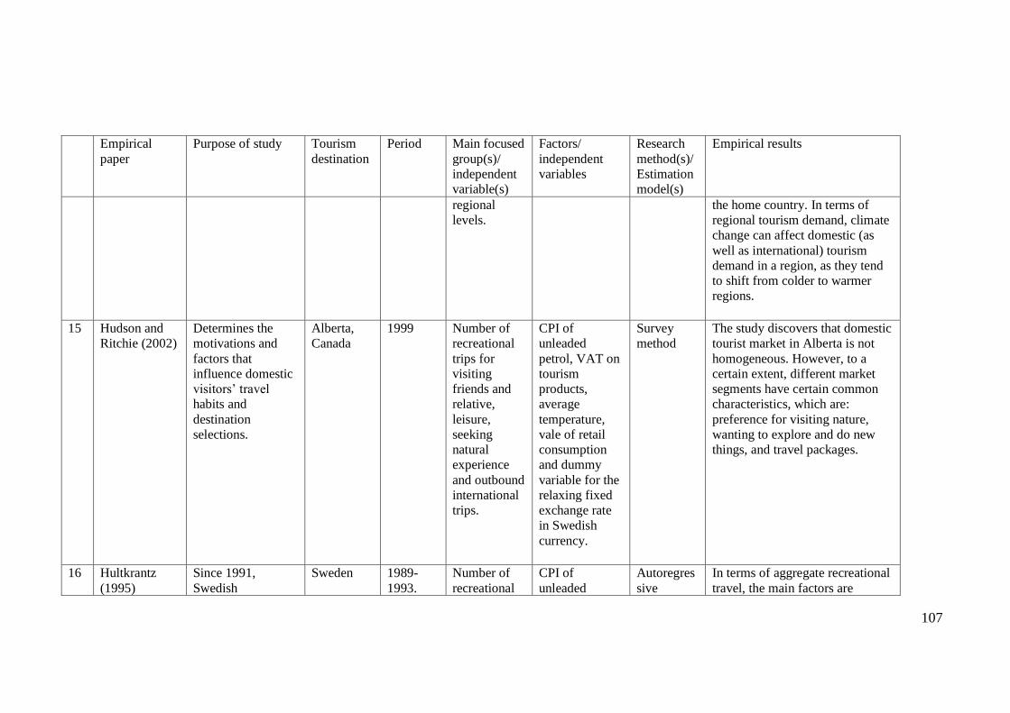
107
Empirical
paper Purpose of study Tourism
destination
Period Main focused
group(s)/
independent
variable(s)
Factors/
independent
variables
Research
method(s)/
Estimation
model(s)
Empirical results
regional
levels.
the home country. In terms of
regional tourism demand, climate
change can affect domestic (as
well as international) tourism
demand in a region, as they tend
to shift from colder to warmer
regions.
15 Hudson and
Ritchie (2002) Determines the
motivations and
factors that
influence domestic
visitors‟ travel
habits and
destination
selections.
Alberta,
Canada 1999 Number of
recreational
trips for
visiting
friends and
relative,
leisure,
seeking
natural
experience
and outbound
international
trips.
CPI of
unleaded
petrol, VAT on
tourism
products,
average
temperature,
vale of retail
consumption
and dummy
variable for the
relaxing fixed
exchange rate
in Swedish
currency.
Survey
method The study discovers that domestic
tourist market in Alberta is not
homogeneous. However, to a
certain extent, different market
segments have certain common
characteristics, which are:
preference for visiting nature,
wanting to explore and do new
things, and travel packages.
16 Hultkrantz
(1995) Since 1991,
Swedish
Sweden 1989-
1993. Number of
recreational
CPI of
unleaded
Autoregres
sive
In terms of aggregate recreational
travel, the main factors are

108
Empirical
paper Purpose of study Tourism
destination
Period Main focused
group(s)/
independent
variable(s)
Factors/
independent
variables
Research
method(s)/
Estimation
model(s)
Empirical results
government has
imposed tax
reforms that
increased the prices
of goods and
services as well as
interest rates.
Concerning the
effects of new tax
systems on
Swedish tourism
industry, this paper
investigates how
the demand for
recreational travel
affected under this
situation.
trips for
visiting
friends and
relative,
leisure,
seeking
natural
experience
and outbound
international
trips.
petrol, VAT on
tourism
products,
average
temperature,
value of retail
consumption
and dummy
variable for the
relaxing fixed
exchange rate
in Swedish
currency.
Distributiv
e Lag
(ARDL)
approach
temperature, working time, VAT
prices and retail consumption.
However, the effect of petrol
price is significant only for the
data on leisure and outbound
travel. The author also employs
dynamic response analysis to
investigate the impacts of tax
reforms on the recreational travel
demand. The empirical evidence
shows that the impacts affect
those trips which visit friends and
relatives and experience trips.
Furthermore, the new tax system
had significant and negative
effects on the recreational travel
expenditure in 1991 as well as in
1993.
17 Huybers, T.
(2003) To examine the
characteristic of
potential tourists
from Melbourne,
Australia, choosing
a destination for
short-break
Australia
destination
s are:
Intrastate –
Goldfields
of Victoria,
Great
2002
(Survey
data)
Individual‟s
utility of
travelling to a
destination.
Amenities,
crowdedness,
travel activities,
event (or
festival),
expenditure per
person, season,
Survey
method
[Logit
nested
model]
Income and age are the most
important choice determinants for
tourists from Melbourne. Trip
expenditure has a negative impact
on the utility and choice of a
destination. Other determinants,
such as the quality of

109
Empirical
paper Purpose of study Tourism
destination
Period Main focused
group(s)/
independent
variable(s)
Factors/
independent
variables
Research
method(s)/
Estimation
model(s)
Empirical results
holiday.
Ocean
Road,
Morningto
n
Peninsula,
and Phillip
Island.
Interstate –
Canberra
and
Sydney.
and
transportation
time and
distance.
accommodation, repetition of
destination, crowdedness and
transport mode, influence the
tourists‟ utility. However, the
distance of travel and festival at a
destination have no impact on the
tourists‟ choice of destination.
18 Kang and Tan
(2004) Examines the
determinants of
domestic travel
frequency in
Malaysia.
Malaysia Decembe
r 2001-
February
2002
(Survey
data)
Number of
domestic
trips by
residents
from Penang
to other states
of Malaysia.
Age, household
income,
number of rest
days, average
number of day
spent,
household size,
race, gender,
education level
and travelling
environment.
OLS [Tobit
model] The study shows that age, race,
education-level, and average
number of rest days significantly
influence domestic travel
frequency in Malaysia.
Specifically, the older residents,
Chinese, highly educated and
higher number of days spent on
trips increase the frequency of
domestic travel. Household
income is negative correlated
with domestic travel frequency
but it is not statistically
significant. The empirical results

110
Empirical
paper Purpose of study Tourism
destination
Period Main focused
group(s)/
independent
variable(s)
Factors/
independent
variables
Research
method(s)/
Estimation
model(s)
Empirical results
should be treated with caution
because error terms of the model
are tested to be non-normality.
19 Kim and Ngo
(2001) Investigates
spillover effects
among the shocks
of three domestic
airflight routes
data: Brisbane-
Melbourne,
Sdyney-Melbourne
and Sydney-
Brisbane.
Australia 1990-
2000 Number of
airline
passengers
for each
route.
Lagged
dependent
variable and
number of
airline
passengers for
other routes.
Johansen
maximum
likelihood
and
bootstrap
method,
Johansen
cointegrati
on analysis,
VAR,
ECM and
impulse
response
analysis,
Holt-
Winters
methods
and
SARIMA.
The data on three major
Australian airflight routes
(Brisbane-Melbourne, Sydney-
Melbourne and Sydney-Brisbane)
exhibit a stochastic trend
deterministic seasonality. Impulse
response analysis shows that the
data on Sydney-Melbourne route
have significant influences on the
other routes in the short-run. In
the long-run, these three airflight
routes tend to move together. In
terms of forecasting, the evidence
found that univariate models
generate more accurate forecasts
than multivariate models.
20 Kim and Qu
(2002) Examines factors
affecting domestic
South
Korea 1976-
1996 Domestic
travel
Per Capita
GNP, family
OLS
[Principal
The results based on OLS create
multicollinearity issues. However,

111
Empirical
paper Purpose of study Tourism
destination
Period Main focused
group(s)/
independent
variable(s)
Factors/
independent
variables
Research
method(s)/
Estimation
model(s)
Empirical results
Korean tourist
expenditure per
person.
expenditure
per person in
US dollar.
size, number of
cars per
household,
number of
working hours
per week,
number of
years of
education, and
exchange rate.
component
(PC) and
Ridge
regressions
]
using PC and Ridge regressions,
the estimations are significant and
have correct signs. Based on the
study, all variables are significant
except exchange rate.
21 Kim et al.
(2007) Understands
domestic tourism in
North Korea.
North
Korea 2004 Number of
North Korean
defectors in
South Korea.
Motives of
trips, types of
transportation
used,
characteristics
of North
Korean travel
activities, and
North Koreans‟
perceptions of
travel
constraints.
Survey
method The study finds that domestic
tourism demand in North Korea is
strongly controlled by the
country‟s communist ideology.
Apparently, the North Koreans
perceived that the most important
purpose of domestic trips is to
visit friends, relatives and
nationalist places. Furthermore,
the study finds that domestic
tourism in North Korea is not an
important activity for the local
residents because there is little
time for leisure after work and the
transportation facilities in North

112
Empirical
paper Purpose of study Tourism
destination
Period Main focused
group(s)/
independent
variable(s)
Factors/
independent
variables
Research
method(s)/
Estimation
model(s)
Empirical results
Korea are poor and insufficient.
22 Koenig and
Bischoff
(2003)
Examines the
seasonal pattern for
different types of
domestic tourism
demand in UK.
Wales, UK 1994-
2000 Number of
overnight
trips taken by
domestic
visitors.
Not stated. Coefficient
of
variation,
Gini
coefficient,
concentrati
on index,
seasonal
decomposit
ion
approach
and
amplitude
ratio
Wales short holidays are highly
seasonal, with sharp peaks in
April, May, July and August.
Visiting friends and relatives
(VFR) are the least seasonal
concentrated for Wales‟s tourism.
Furthermore, the peak season for
business trips in Wales coincides
with the peak season for holidays. Among domestic regions in UK,
data on domestic long holiday
trips in Wales have a higher
seasonal pattern than the rest of
UK regions and Scotland.
23 Lundgren et
al. (2006) Develops a micro-
simulation model
to assess the travel
characteristics and
behaviour of
domestic leisure
tourism in Sweden.
Sweden 1960-
2002
(Survey
data)
Number of
trips. Age, income,
gender,
university
degree (or
education
level),
household
demographic,
gender,
Poisson
regression
[Multinomi
al logistic
model]
Propensity to travel decreases
with age. Medium income earners
are more likely to travel than
those high income earners. High
educated persons tend to travel
more. Men travelled more than
women. Singles tend to travel
more than couples and people
with children. Domestic ski

113
Empirical
paper Purpose of study Tourism
destination
Period Main focused
group(s)/
independent
variable(s)
Factors/
independent
variables
Research
method(s)/
Estimation
model(s)
Empirical results
characteristic of
destination
(city, town or
village) and
region.
tourism in Sweden is less
sensitive to distance. However,
domestic tourists, who travel for
sun and bath, tend to be sensitive
to distance.
24 Mena et al.
(2004) Evaluates
ASEAN‟s
demography to
uncover the
potential demand
for domestic
tourism in the
ASEAN countries.
Brunei,
Cambodia,
Indonesia,
Malaysia,
Myanmar,
Laos,
Philippine,
Singapore,
Thailand,
and
Vietnam.
2002 Number of
projected
population
and growth
rate in
ASEAN
countries
from 2000 to
2050.
Fertility, life
expectancy,
infant mortality
rate and the
degree of
urbanization.
The
analysis
was based
on
secondary
data which
was
obtained
from the
United
Nations
(UN).
Increasing urbanization in
ASEAN can create a stronger
push for city dwellers to travel
domestically. Domestic tourism
demand in ASEAN can boost in
the future when the rate of
fertility is projected to decline.
This indicates that less people
bear children and they may have
more leisure time and
discretionary income to spend on
touristic activities.
25 Rule et al.
(2003) Examines the
characteristics of
South African
visitors who visited
friends and
relatives (VFR).
South
Africa 2001 Number of
domestic
tourists by
purposes of
visits.
Demographic
and types of
expenditure.
Survey
method In South Africa, more than half of
the domestic tourism market is
the travellers who visit friends
and relatives. This group of
domestic tourists spent an annual
total of R4.5 billion and most of
their expenditure contributes to

114
Empirical
paper Purpose of study Tourism
destination
Period Main focused
group(s)/
independent
variable(s)
Factors/
independent
variables
Research
method(s)/
Estimation
model(s)
Empirical results
transportation and food.
26 Salman et al.
(2007) Determines the
domestic demand
for tourism in
Sweden.
Sweden 1980-
1998 Number of
nights spent
by domestic
residents in
Sweden.
CPI, average
personal
disposable
income,
temperature
(proxy for
weather
conditions) in
Sweden,
nominal
exchange rate,
lagged
dependent
variables,
dummy
variable for the
Chernobyl
nuclear
disaster, and
seasonal
dummies.
OLS The study finds that the CPI,
weather conditions, lagged
dependent variables, and seasonal
dummies have significantly
influences on domestic tourism
demand in Sweden.
27 Seddighi and
Shearing
To determine
whether tourism in
Northumbri
a, North
1972-
1994 Total
domestic
Relative prices
(ratio of
Cointegrati
on analysis
The results show that expenditure
on domestic tourism is influenced

115
Empirical
paper Purpose of study Tourism
destination
Period Main focused
group(s)/
independent
variable(s)
Factors/
independent
variables
Research
method(s)/
Estimation
model(s)
Empirical results
(1997) Northumbria is
potential for
economic
development in the
region. To do this,
modelling the
demand for tourism
in Northumbria is
carried out for
forecasting
purposes.
East
England tourism
expenditure tourism prices
to total
consumer
expenditure)
and real total
disposable
income.
and error-
correction
model
by relative price of tourism and
real total disposable income.
Furthermore, there is a long-run
relationship between the
expenditure and its economic
determinants.
28 Sung et al.
(2001) Examines the
factors that
influence
travellers‟ types of
trips.
USA 1994
(Survey
data)
Types of trips
(i.e. Visiting
friends and
relatives
(VFR),
business,
recreation,
other, and
day-trips)
Income,
expenditure
(lodging, food,
transportation
and
entertainment);
Trip
characteristics
(mode of
transportation
and length of
trips);
Household
demographics
Multivariat
e ANOVA,
cross-
sectional
stepwise
regression
Multivariate ANOVA results
show that household income,
demographic, socio-cultural, trip
characteristics and travel
expenditure are shown
statistically significant. However,
stepwise regression results reveal
that number of household income
earners does not affect the
travellers‟ types of trips.
Travellers from different regions
have effects on the choice of
trips.

116
Empirical
paper Purpose of study Tourism
destination
Period Main focused
group(s)/
independent
variable(s)
Factors/
independent
variables
Research
method(s)/
Estimation
model(s)
Empirical results
(family status,
marital status,
earning
composition,
age and
gender); and
socio-cultural
characteristics
(education,
occupation,
race and
region).
29 Tsartas et al.
(2001) Evaluates the
quality and
characteristics of
domestic tourism in
Greece.
Greece 1999 Two groups
of
respondents:
tourism
suppliers and
domestic
residents who
were
travelling in
Greece.
Types of tourist
activities,
demographic,
social and
economic
characteristics.
Survey
method Income and education level make
a positive contribution to
domestic tourism in Greece.
Domestic tourists in Greece have
different motives of travel. The
study also finds that the demand
is dynamic in both urban and
rural regions. The highly
demanded tourist activities by
domestic residents in Greece are
curative, mountaineering, skiing
and ecotourism. Domestic tourists
in Greece travel mostly during

117
Empirical
paper Purpose of study Tourism
destination
Period Main focused
group(s)/
independent
variable(s)
Factors/
independent
variables
Research
method(s)/
Estimation
model(s)
Empirical results
summer.
30 Walsh and
Swain (2004) Examines why
modern Chinese
domestic tourists
attracted to the
ethnic tourism in
Yunnan.
Yunnan,
China Not
stated Chinese
domestic
tourists in
Yunnan.
Not applicable Qualitative
research
method
The main motivations for the
domestic visitors participating in
the ethnic tourism in Yunnan are
nostalgia, exploration, personal
liberation, culture and self-
identification.
31 Wang and Qu
(2004) Compares the
characteristics of
domestic tourism
between China and
the USA.
China and
the USA. Not
stated. Number of
domestic
tourists in
China and the
USA.
Tourists‟
source of
information,
types of
transportation
and
accommodation
, tourists‟ travel
activities and
spending
patterns, and
government
involvement in
domestic
tourism.
Based on
survey data
published
in
statistical
reports ad
research
papers
from both
countries.
Internet has become a main
source of information for
domestic tourists. Chinese
domestic tourists spend less on
travelling. This could relate to the
poor quality of Chinese domestic
tour products. Also, Chinese
domestic tourists tend to stay at
relatives‟ or friends‟ places,
whereas US domestic tourists
prefer accommodating in hotels
or motels.
32 Wang et al. Investigates the USA 2001 Total Socio- Survey Household income and length of

118
Empirical
paper Purpose of study Tourism
destination
Period Main focused
group(s)/
independent
variable(s)
Factors/
independent
variables
Research
method(s)/
Estimation
model(s)
Empirical results
(2006) effects of socio-
demographic,
travel-related and
psychographic
variables on
different types of
travel expenditures
by USA residents
in Mid-Western
region.
expenditure,
and other
expenditure
on lodging,
meals and
restaurant,
attraction and
festival,
entertainment
, shopping
and
transportation
demographic
(gender, age,
marital status,
number of
children and
household
income), travel
related (number
of travel group,
number of
adults and
children, first-
time versus
repeat travel,
length of stay
and travel
distance),
Psychographic
(stability or
excitement,
passive or
active, self or
family,
education level,
traditional or
want new
things)
method [Multiple
regression
analysis]
stay are found to be the most
significant impacts on most
categories of expenditure. For
trip-related variables, the level of
importance varies depending on
expenditure categories. For
instance, travel distance affects
shopping, transportation and total
expenditure, while number of
adults influences expenditure on
lodging, meals and restaurants,
shopping and transportation.

119
Chapter 3
The determinants of domestic and
international tourism: A review and
comparison of findings
The theory of consumer demand posits that household income and tourism prices are
the main determinants that influence tourism demand. Furthermore, other factors such
as marketing expenditure and tourist preferences also play an important role in
determining tourism demand.
This thesis reviews the empirical results which are published in the tourism and
economic journals between 1995 and 2008. The main intention is to review the
empirical findings of domestic and international tourism demand studies. Given that
domestic and international visitors often have different travel expectations and
experiences even though they have visited the same destination [Bonn et al. (2005),
Carr (2002) and Yuksel (2004)], it is worthwhile to investigate whether different
tourism destinations attract visitors with different economic characteristics.
In the past, Crouch (1994a) conducted a review of findings based on 85 empirical
studies of international tourism demand from 1960 to 1992. The author evaluated the
demand elasticities across different studies. Nevertheless, the empirical research from
1993 onwards has not been reviewed since then. Furthermore, the tourism literature has
little or virtually no discussion about whether domestic and international visitors
respond differently to the changes in economic conditions.
From the overall review of the literature, the demand determinants used in domestic
tourism analysis are slightly different from international tourism. This thesis finds that
international tourism demand is strongly affected by household income, tourism prices,
marketing expenditure, lagged dependent variables, destination price indices (DPI),
tourism supply, trade volume and one-off events, whilst domestic tourism demand is

120
significantly influenced by domestic household income, domestic prices, transportation
costs, exchange rate, working hours, lagged dependent variables and one-off events.
3.1 Income
Income is the most important factor which determines the economic capability of a
visitor to travel to a destination. Because of its importance, most of the empirical papers
have included income variables in tourism demand analyses. In terms of determining a
proxy for the income variable, Lim (1997 and 2006) argued that discretionary income
would be appropriate because consumers would choose recreational travel after
deducting the expenditure on necessities. However, due to the limitations of obtaining a
reliable data for discretionary income, Lim discovered that most tourism researchers
have employed other income proxies, such as nominal or real disposable and national
income, gross domestic products, gross national products and real average wage per
employee.
In 1994, Crouch‟s meta-analysis revealed that the estimated income elasticities of
international tourism demand were typically above unity, indicating that foreign travel
is a luxury product [Crouch (1994a)]. In more recent years, the majority of the empirical
papers which appeared between 1995 and 2008 supported Crouch‟s findings. The
summary of the tourism demand literature in Table 3.1 confirms that most of the income
elasticities of international tourism demand are above one. For instance, tourists from
Norway and Sweden to Denmark are highly sensitive to the changes in their income
[Jensen (1998) and Song et al. (2003a)]. Furthermore, the income elasticities of
European tourists travelling to UK range from 1.78 to 2.82, indicating that UK is a
luxury tourism product for most of European tourists. Similarly, the income elasticities
for US tourists travelling to Asia, Australia, New Zealand, Scotland and Switzerland
exceed unity, implying that US tourists considered these destinations as luxury tourism
products [Jensen (1998), Kim and Song (1998), Kulendran and Divisekara (2007),
Kulendran and Wilson (2000), Luzzi and Fluckiger (2003), Narayan (2004) and Turner
and Witt (2001b)].
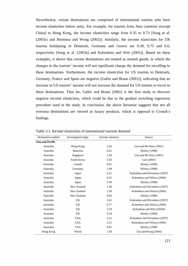
121
Nevertheless, certain destinations are comprised of international tourists who have
income elasticities below unity. For example, for tourists from Asia countries (except
China) to Hong Kong, the income elasticities range from 0.35 to 0.73 [Song at al.
(2003c) and Hiemstra and Wong (2002)]. Similarly, the income elasticities for UK
tourists holidaying in Denmark, Germany and Greece are 0.39, 0.75 and 0.6,
respectively [Song et al. (2003a) and Kulendran and Witt (2001)]. Based on these
examples, it shows that certain destinations are treated as normal goods, in which the
changes in the tourists‟ income will not significant change the demand for travelling to
these destinations. Furthermore, the income elasticities for US tourists to Denmark,
Germany, France and Spain are negative [Gallet and Braun (2001)], indicating that an
increase in US tourists‟ income will not increase the demand for US tourists to travel to
these destinations. Thus far, Gallet and Braun (2001) is the first study to discover
negative income elasticities, which could be due to the gradual switching regression
procedure used in the study. In conclusion, the above literature suggests that not all
overseas destinations are viewed as luxury products, which is opposed to Crouch‟s
findings.
Table 3.1. Income elasticities of international tourism demand
Destination studied Investigated origin Income elasticity Source
Asia and Pacific
Australia Hong Kong 2.26 Lim and McAleer (2001)
Australia Malaysia 0.61 Morley (1998)
Australia Singapore 1.59 Lim and McAleer (2001)
Australia South Korea 5.95 Lim (2004)
Australia Canada 0.61 Morley (1998)
Australia Germany 1.48 Morley (1998)
Australia Japan 6.21 Kulendran and Divisekera (2007)
Australia Japan 0.25 Kulendran and Wilson (2000)
Australia Japan 2.94 Morley (1998)
Australia New Zealand 1.46 Kulendran and Divisekera (2007)
Australia New Zealand 1.58 Kulendran and Wilson (2000)
Australia New Zealand 0.04 Morley (1998)
Australia UK 2.41 Kulendran and Divisekera (2007)
Australia UK 0.77 Kulendran and Wilson (2000)
Australia UK 2.29 Kulendran and Witt (2003b)
Australia UK 0.34 Morley (1998)
Australia USA 3.13 Kulendran and Divisekera (2007)
Australia USA 2.21 Kulendran and Wilson (2000)
Australia USA 0.01 Morley (1998)
Hong Kong World 1.84 Tan and Wong (2004)

122
Destination studied Investigated origin Income elasticity Source
Hong Kong Australia 2.24 Hiemstra and Wong (2002)
Hong Kong China 1.52 Song et al. (2003c)
Hong Kong China 1.01 Hiemstra and Wong (2002)
Hong Kong India 0.65 Song et al. (2003c)
Hong Kong Korea 0.73 Song et al. (2003c)
Hong Kong Malaysia 0.54 Song et al. (2003c)
Hong Kong Singapore 0.45 Song et al. (2003c)
Hong Kong Taiwan 0.35 Hiemstra and Wong (2002)
Hong Kong Taiwan 0.85 Song et al. (2003c)
Hong Kong Thailand 0.52 Song et al. (2003c)
Hong Kong Canada 1.52 Song et al. (2003c)
Hong Kong France 2.06 Song and Wong (2003)
Hong Kong Germany 1.18 Song and Wong (2003)
Hong Kong Germany 1.05 Song et al. (2003c)
Hong Kong Japan 0.32 Song et al. (2003c)
Hong Kong UK 2.08 Song and Wong (2003)
Hong Kong UK 1.04 Song et al. (2003c)
Hong Kong USA 0.56 Hiemstra and Wong (2002)
Hong Kong USA 2.91 Song and Wong (2003)
Hong Kong USA 0.54 Song et al. (2003c)
Hong Kong World 1.84 Tan and Wong (2004)
Indonesia Australia 0.83 Webber (2001)
Japan Australia 0.69 Webber (2001)
Korea Japan 1.11 Song and Witt (2003)
Korea UK 1.42 Song and Witt (2003)
Malaysia Australia 0.48 Webber (2001)
Malaysia World 1.49 Tan et al. (2002a)
New Zealand Australia 0.55 Webber (2001)
New Zealand Japan 2.61 Lim et al. (2008)
New Zealand USA 2.13 Turner and Witt (2001b)
Philippines Australia 0.91 Webber (2001)
Singapore Australia 0.37 Webber (2001)
South Korea Germany 1.53 Kim and Song (1998)
South Korea Japan 2.54 Kim and Song (1998)
South Korea UK 2.08 Kim and Song (1998)
South Korea USA 3 Kim and Song (1998)
Taiwan Japan 1.50 Lim et al. (2008)
Taiwan Japan 3.35 Wang (2008)
Thailand Australia 1.45 Song et al. (2003b)
Thailand Australia 1.21 Webber (2001)
Thailand Korea 0.57 Song et al. (2003b)
Thailand UK 2.32 Song et al. (2003b)
Europe
Austria UK 2.72 Song et al. (2000)
Austria USA 0.16 Gallet and Braun (2001)
Denmark Norway 1.34 Jensen (1998)
Denmark Norway 1.34 Song et al. (2003a)

123
Destination studied Investigated origin Income elasticity Source
Denmark Sweden 2.72 Jensen (1998)
Denmark Sweden 2.63 Song et al. (2003a)
Denmark UK 0.5 Jensen (1998)
Denmark UK 0.39 Song et al. (2003a)
Denmark USA -0.49 Gallet and Braun (2001)
Denmark USA 2.77 Jensen (1998)
Denmark USA -1.07 Song et al. (2003a)
France UK 2.12 Song et al. (2000)
France USA -0.64 Gallet and Braun (2001)
Germany UK 0.75 Kulendran and Witt (2001)
Germany UK 2.26 Song et al. (2000)
Germany USA -0.27 Gallet and Braun (2001)
Greece Germany 2.16 Dritsakis (2004)
Greece UK 6.03 Dritsakis (2004)
Greece UK 0.6 Kulendran and Witt (2001)
Greece UK 2.17 Song et al. (2000)
Irish Republic UK 2.66 Song et al. (2000)
Italy UK 1.74 Song et al. (2000)
Netherlands UK 1.33 Kulendran and Witt (2001)
Netherlands UK 2.45 Song et al. (2000)
Portugal France 2.43 Daniel and Ramos (2002)
Portugal Germany 2.03 Daniel and Ramos (2002)
Portugal Netherlands 2.98 Daniel and Ramos (2002)
Portugal UK 1.71 Kulendran and Witt (2001)
Russia World 7.89 Algieri (2006)
Scotland France 1.82 Eugenio-Martin et al. (2005)
Scotland Germany 2.93 Eugenio-Martin et al. (2005)
Scotland USA 1.45 Eugenio-Martin et al. (2005)
Spain World 1.4 Garin-Munoz and Amaral (2000)
Spain World 0.48 Garcia-Ferrer and Queralt (1997)
Spain World 3 Jimenez (2002)
Spain UK 0.93 Kulendran and Witt (2001)
Spain UK 2.2 Song et al. (2000)
Spain USA -1.17 Gallet and Braun (2001)
Spain Germany 2.62 Garin-Munoz (2007)
Sun and sea
destinations in Spain
Germany 4.33 Garin-Munoz (2007)
Sweden Germany 0.53 Salman (2003)
Sweden Denmark 0.66 Salman (2003)
Sweden Finland 2 Salman (2003)
Sweden UK 0.01 Salman (2003)
Sweden USA 0.37 Salman (2003)
Switzerland Europe 0.05 Luzzi and Fluckiger (2003)
Switzerland Japan 2.35 Luzzi and Fluckiger (2003)
Switzerland UK 2.03 Song et al. (2000)
Switzerland USA 2.61 Luzzi and Fluckiger (2003)
UK Australia 0.39 Webber (2001)
UK France 2.82 Li et al. (2006)

124
Destination studied Investigated origin Income elasticity Source
UK Greece 1.83 Li et al. (2006)
UK Italy 1.94 Li et al. (2006)
UK Portugal 1.78 Li et al. (2006)
UK Spain 2.22 Li et al. (2006)
UK USA 0.7 Gallet and Braun (2001)
America
USA Japan 2.5 Bonham et al. (2006)
USA UK 1.7 Kulendran and Witt (2001)
USA UK 1 Kulendran and Witt (2001)
USA UK 2 Song et al. (2000)
Rest of the world
Africa Europe -45.14 Naude and Saayman (2005)
Barbados World 0.97 Greenidge (2001)
Croatia World 3.6 Payne and Mervar (2002)
Fiji Australia 3.59 Narayan (2004)
Fiji New Zealand 3.07 Narayan (2004)
Fiji USA 4.36 Narayan (2004)
Guam Japan 1.7 Ismail et al. (2000)
Tunisia France 4.20 Ouerfelli (2008)
Tunisia Germany 1.47 Ouerfelli (2008)
Tunisia Italy 3.64 Ouerfelli (2008)
Tunisia UK 0.76 Ouerfelli (2008)
World UK 3.85 Song et al. (2000)
Note: The income elasticity estimations are extracted from the empirical literature of international tourism demand
during 1995 and 2008. The main purpose of constructing this summary is to compare the income elasticities across different countries or continents. The estimates vary from one study to another, which could be due to different
models and data used. Refer to Appendix 2.1 for further details.
For domestic tourism demand, Athanasopoulos and Hyndman (2008) estimated
negative income elasticity for Australian domestic tourism demand. They argued that a
growth in Australian household income discouraged domestic travel (Table 3.2).
Comparing the income elasticities between domestic and international tourism demand
(Tables 3.1 and 3.2), the literature reveals two surprising findings. First, the income
elasticities of domestic tourism demand in developed countries are higher than that of
outbound tourism. In Australia, Hamal (1996) found that the income elasticity of
Australian domestic tourism demand is 1.74. However, Webber (2001) discovered that
the income elasticities of Australians travelling overseas are below unity. Similarly, in
the UK, the income elasticities of UK tourists travelling to Northumbria, North East
England, is 19.76 whereas it is 6.03 for UK tourists travelling to Greece [Dritsakis

125
(2004) and Seddighi and Shearing (1997)]. Hence, these researches show that, in
developed countries, the demand for domestic tourism responds to the variation of
visitors‟ income more strongly than the demand for outbound tourism.
Second, the income elasticities of domestic tourism demand in emerging countries are
lower than that for outbound tourism. In China, the income elasticity of Chinese
residents travelling domestically is 0.01 [Cai et al. (2001)], but the income elasticities
for Mainland Chinese travelling to Hong Kong ranges from 1.01 to 1.52. Moreover, in
Korea, the income elasticity of Korean residents holidaying within their country is 0.14
[Kim and Qu (2002)], whereas it is 0.73 for Korean tourists travelling to Hong Kong.
Hence, in contrast to the case of Australia and UK above, changes in household income
in emerging countries would have a large impact on the demand for overseas travel but
less effect on domestic tourism demand.
Table 3.2. Income elasticities of domestic tourism demand
Destination studied Income elasticity Source
Africa 55.5 Naude and Saayman (2005)
Australia -43.71 Athanasopoulos and Hyndman (2008)
Australia 1.74 Hamal (1996)
China 0.01 Cai et al. (2001)
Korea 0.14 Kim and Qu (2002)
Northumbria, North East England 19.76 Seddighi and Shearing (1997)
Note: The income elasticity estimations are obtained from the empirical literature of domestic tourism
demand during 1995 and 2008. For Australia case, the elasticities generated by Athanasopoulos and
Hyndman (2008) and Hamal (1996) are distinct significantly from each other. The reason could be related
to different models and examined period used in both studies. Refer to Appendix 2.2 for further details.
3.2 Tourism prices
In the literature of international tourism demand, it is widely acknowledged that tourism
prices can be categorized into three types, namely relative prices, exchange rates and
transportation costs [Crouch (1994a) and Lim (2006)]. Relative prices can be further
divided into own- and cross-price effects. The former is expressed as the ratio of prices
in the destination to prices in the origin country, whereas the latter is defined as the ratio

126
of prices in the destination to prices in competing destinations. The data on relative
prices used in the tourism literature is the price adjusted by the consumer price index
which excludes the effects of inflation. In other words, the inflation-adjusted relative
price can be termed as a real exchange rate. Apart from that, the literature also
highlighted that consumers are more aware of nominal exchange rates than the costs of
living at their destinations [Witt and Witt (1995)]. Therefore, exchange rates have been
used widely in the empirical literature as a proxy for tourism prices. Lastly, Crouch
(1994a) argued that many prospective tourists would first consider the price of
transportation costs before they determine any travel decisions. Therefore,
transportation costs have become one of the important demand determinants for
international travel.
Crouch (1994b) reviewed the empirical papers from 1960 to 1992 and discovered that
long-haul tourism is less sensitive to changes in tourism prices than short-haul tourism.
The author further argued that long-haul tourists are less aware of foreign prices in long
distant destinations. This thesis aligns with Crouch‟s findings. In Table 3.3, it is
presented that the relative price elasticities for long-haul tourists are below unity. For
instance, the price elasticities for Canadian tourists to Hong Kong range between -0.26
and -0.8 [Song and Wong (2003) and Song et al. (2003c)]. Furthermore, the price
elasticities for US tourists to Hong Kong, South Korea and Austria are -0.87, -0.55 and
-0.15, respectively [Gallet and Braun (2001), Song and Witt (2003) and Song and Wong
(2003)].
On the other hand, tourism researchers also discovered that the relative price elasticities
for short-haul tourists are above unity. For instance, in the case of German tourists
travelling to Denmark, the price elasticities range between -1.07 and -1.18 [Jensen
(1998) and Song et al. (2003a)]. Moreover, several empirical studies also showed that
UK tourists are sensitive to tourism price changes in Austria, Germany, France, Italy
and Sweden [Kulendran and Witt (2001), Patsouratis et al. (2005), Salman (2003) and
Song et al. (2000)]. Similarly, Ouerfelli (2008) found that the price elasticities of
European international travel to Tunisia range between -1.51 and -8.34.
Table 3.4 presents a summary of exchange rate elasticities of international tourism
demand. It measures the influence of exchange rates on tourist arrivals to a destination.

127
Table 3.3. Relative price elasticities of international tourism demand
Destination studied Investigated origin Relative price
elasticity
Source
Asia and the Pacific
Australia Canada -0.35 Morley (1998)
Australia Malaysia -1.20 Morley (1998)
Australia South Korea -6.1 Lim (2004)
Australia Germany -1.18 Morley (1998)
Australia Japan -0.37 Kulendran and Divisekera (2007)
Australia Japan -2.87 Morley (1998)
Australia New Zealand -0.94 Kulendran and Divisekera (2007)
Australia New Zealand -0.25 Kulendran and Wilson (2000)
Australia New Zealand -0.24 Kulendran and Witt (2003)
Australia New Zealand -0.56 Morley (1998)
Australia UK -0.32 Kulendran and Divisekera (2007)
Australia UK -0.76 Morley (1998)
Australia USA -0.3 Kulendran and Divisekera (2007)
Australia USA -0.46 Morley (1998)
Hong Kong World -0.85 Tan and Wong (2004)
Hong Kong Australia -0.34 Hiemstra and Wong (2002)
Hong Kong Australia -0.42 Song and Wong (2003)
Hong Kong Australia -0.53 Song et al. (2003c)
Hong Kong Canada -0.8 Song and Wong (2003)
Hong Kong Canada -0.26 Song et al. (2003c)
Hong Kong China -0.25 Hiemstra and Wong (2002)
Hong Kong China -0.4 Song et al. (2003c)
Hong Kong India -0.47 Song et al. (2003c)
Hong Kong Indonesia -0.05 Song et al. (2003c)
Hong Kong Malaysia -0.06 Song et al. (2003c)
Hong Kong Singapore -0.42 Song et al. (2003c)
Hong Kong Taiwan -0.69 Song et al. (2003c)
Hong Kong Thailand -0.5 Song et al. (2003c)
Hong Kong France -0.36 Song and Wong (2003)
Hong Kong France -0.32 Song et al. (2003c)
Hong Kong Germany -0.4 Song et al. (2003c)
Hong Kong UK -0.23 Hiemstra and Wong (2002)
Hong Kong UK -0.54 Song and Wong (2003)
Hong Kong UK -0.25 Song et al. (2003c)
Hong Kong USA -0.87 Song and Wong (2003)
Indonesia Australia -0.31 Webber (2001)
Japan Australia -0.5 Webber (2001)
Korea Germany -0.29 Song and Witt (2003)
Korea UK -0.02 Song and Witt (2003)
Malaysia World -0.55 Tan et al. (2002a)
Malaysia Australia -0.15 Webber (2001)
New Zealand Australia -0.31 Webber (2001)
Singapore Australia -0.53 Webber (2001)
South Korea UK -0.3 Kim and Song (1998)
South Korea USA -0.59 Song and Witt (2003)
South Korea USA -0.54 Kim and Song (1998)
Taiwan Japan 18.31 Wang (2008)*
Thailand Australia -1.37 Song et al. (2003b)
Thailand Australia -1.86 Webber (2001)
Thailand Singapore -0.81 Song et al. (2003b)
Thailand Japan -1.05 Song et al. (2003b)
Thailand USA -1 Song et al. (2003b)
Europe
Austria UK -2.09 Song et al. (2000)
Austria USA -0.15 Gallet and Braun (2001)

128
Destination studied Investigated origin Relative price
elasticity
Source
Belgium/Luxembourg UK -0.53 Song et al. (2000)
Denmark Germany -1.07 Jensen (1998)
Denmark Germany -1.18 Song et al. (2003a)
Denmark Holland -5.85 Jensen (1998)
Denmark Norway -0.62 Song et al. (2003a)
Denmark Sweden -1.22 Jensen (1998)
Denmark Sweden -0.68 Song et al. (2003a)
Denmark Netherlands -1.29 Song et al. (2003a)
Denmark UK -0.48 Jensen (1998)
Denmark UK -0.89 Song et al. (2003a)
Denmark USA -1.07 Jensen (1998)
Denmark USA -0.56 Song et al. (2003a)
France UK -1.08 Song et al. (2000)
Germany UK -2.3 Kulendran and Witt (2001)
Germany UK -1.25 Song et al. (2000)
Germany USA -0.42 Gallet and Braun (2001)
Greece France -1.08 Patsouratis et al. (2005)
Greece Italy -1.43 Patsouratis et al. (2005)
Greece UK -0.93 Kulendran and Witt (2001)
Greece UK -1.69 Patsouratis et al. (2005)
Irish Republic UK -0.95 Song et al. (2000)
Italy UK -1.01 Song et al. (2000)
Italy USA -0.52 Gallet and Braun (2001)
Netherlands UK -0.23 Song et al. (2000)
Portugal France -2.92 Daniel and Ramos (2002)
Portugal Germany -1.54 Daniel and Ramos (2002)
Portugal Spain -0.22 Daniel and Ramos (2002)
Portugal Netherlands -1.6 Daniel and Ramos (2002)
Portugal UK -3.04 Daniel and Ramos (2002)
Portugal UK -0.68 Kulendran and Witt (2001)
Russia World -1.47 Algieri (2006)
Spain World -0.3 Garin-Munoz and Amaral (2000)
Spain World -0.55 Garcia-Ferrer and Queralt (1997)
Spain UK -2.99 Kulendran and Witt (2001)
Spain UK -0.5 Song et al. (2000)
Spain Germany -6.62 Garin-Munoz (2007)
Non-sun and non-sea
destinations in Spain
Germany -0.31 Garin-Munoz (2007)
Sun and sea destinations
in Spain
Germany -0.74 Garin-Munoz (2007)
Sweden Germany -0.91 Salman (2003)
Sweden Denmark -0.15 Salman (2003)
Sweden Norway -0.89 Salman (2003)
Sweden UK -1.62 Salman (2003)
Sweden USA -0.4 Salman (2003)
Switzerland World -2.4 Luzzi and Fluckiger (2003)
Switzerland Japan -0.97 Luzzi and Fluckiger (2003)
Switzerland USA -0.17 Gallet and Braun (2001)
Switzerland USA -0.02 Luzzi and Fluckiger (2003)
UK France -1.16 Li et al. (2006)
UK Greece -1.96 Li et al. (2006)
UK Italy -1.18 Li et al. (2006)
UK Spain -1.23 Li et al. (2006)
UK USA -0.58 Gallet and Braun (2001)
America
USA Japan -0.34 Bonham et al. (2006)
USA UK -0.5 Kulendran and Witt (2001)
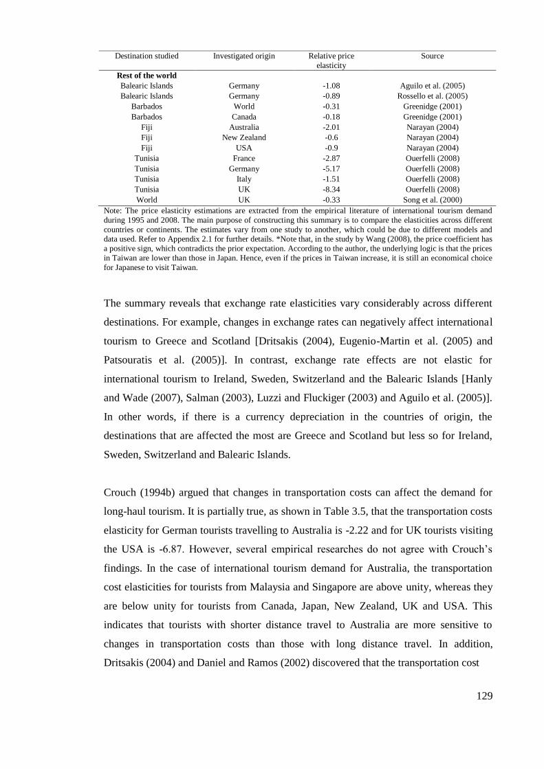
129
Destination studied Investigated origin Relative price
elasticity
Source
Rest of the world
Balearic Islands Germany -1.08 Aguilo et al. (2005)
Balearic Islands Germany -0.89 Rossello et al. (2005)
Barbados World -0.31 Greenidge (2001)
Barbados Canada -0.18 Greenidge (2001)
Fiji Australia -2.01 Narayan (2004)
Fiji New Zealand -0.6 Narayan (2004)
Fiji USA -0.9 Narayan (2004)
Tunisia France -2.87 Ouerfelli (2008)
Tunisia Germany -5.17 Ouerfelli (2008)
Tunisia Italy -1.51 Ouerfelli (2008)
Tunisia UK -8.34 Ouerfelli (2008)
World UK -0.33 Song et al. (2000)
Note: The price elasticity estimations are extracted from the empirical literature of international tourism demand
during 1995 and 2008. The main purpose of constructing this summary is to compare the elasticities across different
countries or continents. The estimates vary from one study to another, which could be due to different models and data used. Refer to Appendix 2.1 for further details. *Note that, in the study by Wang (2008), the price coefficient has
a positive sign, which contradicts the prior expectation. According to the author, the underlying logic is that the prices
in Taiwan are lower than those in Japan. Hence, even if the prices in Taiwan increase, it is still an economical choice
for Japanese to visit Taiwan.
The summary reveals that exchange rate elasticities vary considerably across different
destinations. For example, changes in exchange rates can negatively affect international
tourism to Greece and Scotland [Dritsakis (2004), Eugenio-Martin et al. (2005) and
Patsouratis et al. (2005)]. In contrast, exchange rate effects are not elastic for
international tourism to Ireland, Sweden, Switzerland and the Balearic Islands [Hanly
and Wade (2007), Salman (2003), Luzzi and Fluckiger (2003) and Aguilo et al. (2005)].
In other words, if there is a currency depreciation in the countries of origin, the
destinations that are affected the most are Greece and Scotland but less so for Ireland,
Sweden, Switzerland and Balearic Islands.
Crouch (1994b) argued that changes in transportation costs can affect the demand for
long-haul tourism. It is partially true, as shown in Table 3.5, that the transportation costs
elasticity for German tourists travelling to Australia is -2.22 and for UK tourists visiting
the USA is -6.87. However, several empirical researches do not agree with Crouch‟s
findings. In the case of international tourism demand for Australia, the transportation
cost elasticities for tourists from Malaysia and Singapore are above unity, whereas they
are below unity for tourists from Canada, Japan, New Zealand, UK and USA. This
indicates that tourists with shorter distance travel to Australia are more sensitive to
changes in transportation costs than those with long distance travel. In addition,
Dritsakis (2004) and Daniel and Ramos (2002) discovered that the transportation cost
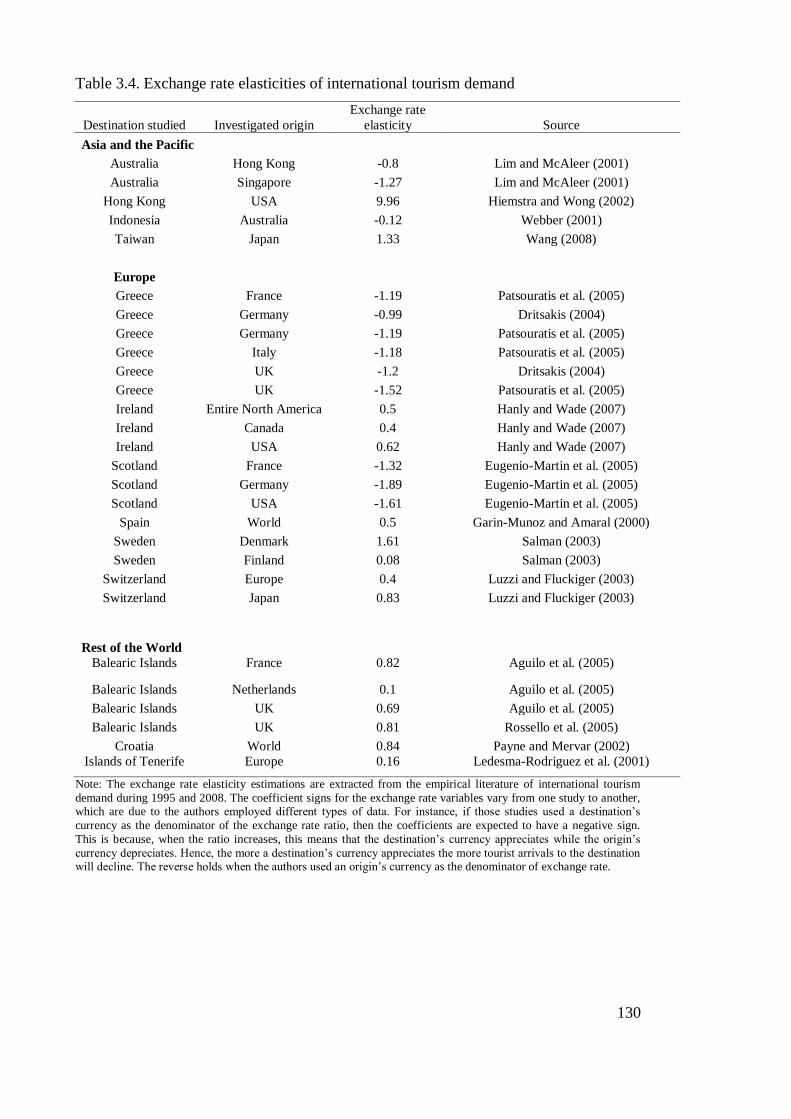
130
Table 3.4. Exchange rate elasticities of international tourism demand
Destination studied Investigated origin
Exchange rate
elasticity Source
Asia and the Pacific
Australia Hong Kong -0.8 Lim and McAleer (2001)
Australia Singapore -1.27 Lim and McAleer (2001)
Hong Kong USA 9.96 Hiemstra and Wong (2002)
Indonesia Australia -0.12 Webber (2001)
Taiwan Japan 1.33 Wang (2008)
Europe
Greece France -1.19 Patsouratis et al. (2005)
Greece Germany -0.99 Dritsakis (2004)
Greece Germany -1.19 Patsouratis et al. (2005)
Greece Italy -1.18 Patsouratis et al. (2005)
Greece UK -1.2 Dritsakis (2004)
Greece UK -1.52 Patsouratis et al. (2005)
Ireland Entire North America 0.5 Hanly and Wade (2007)
Ireland Canada 0.4 Hanly and Wade (2007)
Ireland USA 0.62 Hanly and Wade (2007)
Scotland France -1.32 Eugenio-Martin et al. (2005)
Scotland Germany -1.89 Eugenio-Martin et al. (2005)
Scotland USA -1.61 Eugenio-Martin et al. (2005)
Spain World 0.5 Garin-Munoz and Amaral (2000)
Sweden Denmark 1.61 Salman (2003)
Sweden Finland 0.08 Salman (2003)
Switzerland Europe 0.4 Luzzi and Fluckiger (2003)
Switzerland Japan 0.83 Luzzi and Fluckiger (2003)
Rest of the World
Balearic Islands France 0.82 Aguilo et al. (2005)
Balearic Islands Netherlands 0.1 Aguilo et al. (2005)
Balearic Islands UK 0.69 Aguilo et al. (2005)
Balearic Islands UK 0.81 Rossello et al. (2005)
Croatia World 0.84 Payne and Mervar (2002)
Islands of Tenerife Europe 0.16 Ledesma-Rodriguez et al. (2001)
Note: The exchange rate elasticity estimations are extracted from the empirical literature of international tourism
demand during 1995 and 2008. The coefficient signs for the exchange rate variables vary from one study to another, which are due to the authors employed different types of data. For instance, if those studies used a destination‟s
currency as the denominator of the exchange rate ratio, then the coefficients are expected to have a negative sign.
This is because, when the ratio increases, this means that the destination‟s currency appreciates while the origin‟s
currency depreciates. Hence, the more a destination‟s currency appreciates the more tourist arrivals to the destination will decline. The reverse holds when the authors used an origin‟s currency as the denominator of exchange rate.

131
Table 3.5. Transportation cost elasticities of international tourism demand
Destination studied Investigated origin
Transportation cost
elasticity Source
Asia and the Pacific
Australia Canada -0.56 Morley (1998)
Australia Germany -2.22 Morley (1998)
Australia Hong Kong -0.8 Lim and McAleer (2001)
Australia Japan -0.69 Morley (1998)
Australia Malaysia -1.43 Morley (1998)
Australia New Zealand -0.93
Kulendran and Divisekera
(2007)
Australia New Zealand -0.42 Morley (1998)
Australia Singapore -2.29 Lim and McAleer (2001)
Australia UK -0.32 Morley (1998)
Australia USA -0.03 Morley (1998)
New Zealand USA -0.38 Turner and Witt (2001b)
South Korea Japan -1.75 Kim and Song (1998)
Taiwan Japan -0.95 Wang (2008)
Europe
Greece Germany -0.62 Dritsakis (2004)
Greece UK -1.4 Dritsakis (2004)
Greece UK -1.93 Kulendran and Witt (2001)
Portugal France -1.57 Daniel and Ramos (2002)
Portugal Germany -2.41 Daniel and Ramos (2002)
Portugal Netherlands -1.96 Daniel and Ramos (2002)
Portugal UK -1.27 Daniel and Ramos (2002)
Russia World -5.95 Algieri (2006)
Spain Wold -0.08 Jimenez (2002)
Spain German -0.31 Garin-Munoz (2007)
Spain UK -1.55 Kulendran and Witt (2001)
Non-sun and non-sea
destinations in Spain German -0.31 Garin-Munoz (2007) Sun and sea destinations
in Spain German -0.27 Garin-Munoz (2007)
America
USA UK -6.87 Kulendran and Witt (2001)
Rest of the World
Africa Europe -0.25 Naude and Saayman (2005)
Fiji Australia -1.14 Narayan (2004)
Fiji New Zealand -3.42 Narayan (2004)
Fiji USA -1.98 Narayan (2004)
Islands of Tenerife Europe -0.09
Ledesma-Rodriguez et al.
(2001)
Islands of Tenerife Europe -0.25
Ledesma-Rodriguez et al.
(2001)
Note: The transportation cost elasticity estimations are extracted from the empirical literature of international tourism demand during 1995 and 2008. The main purpose of constructing this summary is to compare the elasticities across
different countries or continents. The estimates vary from one study to another, which could be due to different
models and data used. Refer to Appendix 2.1 for further details.

132
elasticities for European tourists travelling to Greece and Portugal (which are
considered short-haul destinations for Europeans) are highly and negatively elastic.
Table 3.6 exhibits substitute price elasticities for each origin-destination pair. It reveals
that the elasticities for most of the countries in Asia and the Pacific are below one.
Conversely, for European destinations, the majority of the substitute price elasticities
are above unity. This implies that international tourists who travelled to Asia are less
likely to be influenced by prices of substitute destinations. However, the reverse holds
for international tourists who travelled to the European continent. A possible reason
could be that Asian destinations offer stronger competition in price (i.e. cheaper offer
and more value for money) than Europe does.
Several studies also show negative elasticity for prices of tourism in competing
countries. In other words, the negative price elasticity implies a complementary effect.
For instance, the substitute price elasticity for UK tourists travelling to the Irish
Republic is -2.17, implying that the demand for international tourism to the Irish
Republic does not increase even if there is an increase in the prices of competing
destinations [Song et al. (2000)]. Similarly, Eugenio-Martin et al. (2005) also found that
the substitute price elasticity for German tourists visiting Scotland is -2.73.
Furthermore, Narayan (2004) obtained negative substitute price elasticities of
international tourism demand to Fiji. Hence, these empirical findings conclude that an
increase in the price of competing destinations may not indicate an improvement of
international tourism demand to a destination.
In the domestic tourism literature, the rise of tourism prices in a destination can
significantly reduce the number of domestic visitors to the destination. In Australia, if
the price of domestic travel increases by one percent, the number of domestic holiday
visitors will decline between 1.4% and 4.1% [Athanasopoulos and Hyndman (2008) and
Hamal (1996)]. Similarly, Seddighi and Shearing (1997) also found that the number of
domestic tourists in Northumbria, North Englands, will decrease 9% when domestic
travel prices in England increase by one percent. Hence, unlike the international tourism
demand literature where the price elasticities vary according to different studies, almost
all the empirical studies in Table 3.7 conclude that domestic tourism demand is highly
sensitive to changes in domestic tourism prices.

133
Table 3.6. Substitute price elasticities of international tourism demand
Destination studied Investigated
origin
Price of tourism in
competing destinations
Source
Asia and the Pacific
Hong Kong Australia 0.31 Song and Wong (2003)
Hong Kong Australia 0.32 Song et al. (2003c)
Hong Kong Canada 0.52 Song and Wong (2003)
Hong Kong China 1.25 Song et al. (2003c)
Hong Kong India 0.54 Song et al. (2003c)
Hong Kong Philippines 0.71 Song et al. (2003c)
Hong Kong Thailand 0.71 Hiemstra and Wong (2002)
Hong Kong France 0.82 Song and Wong (2003)
Hong Kong France 0.49 Song et al. (2003c)
Hong Kong Germany 1.17 Song and Wong (2003)
Hong Kong UK 0.32 Song et al. (2003c)
Hong Kong UK 0.56 Song and Wong (2003)
Hong Kong UK 0.89 Hiemstra and Wong (2002)
Hong Kong USA 0.3 Song and Wong (2003)
Hong Kong USA 0.33 Song et al. (2003c)
Indonesia Australia 0.28 Webber (2001)
Japan Australia 0.05 Webber (2001)
Korea Germany 0.25 Song and Witt (2003)
Korea USA 0.19 Song and Witt (2003)
New Zealand Australia 0.55 Webber (2001)
Philippines Australia 0.37 Webber (2001)
Singapore Australia 0.47 Webber (2001)
South Korea Japan -0.74 Song and Witt (2003)
Thailand Australia 1.69 Song et al. (2003b)
Thailand Australia 0.69 Webber (2001)
Thailand Korea -0.95 Song et al. (2003b)
Thailand Malaysia 0.77 Song et al. (2003b)
Thailand Singapore 0.8 Song et al. (2003b)
Thailand Japan 0.77 Song et al. (2003b)
Thailand UK 0.83 Song et al. (2003b)
Europe
Austria UK 0.7 Song et al. (2000)
Austria USA 3.28 Gallet and Braun (2001)
Belgium/Luxembourg UK 0.45 Song et al. (2000)
Denmark Germany 2.23 Jensen (1998)
Denmark Netherlands -2.17 Song et al. (2003a)
Denmark Sweden -2.15 Jensen (1998)
Denmark USA 7.81 Gallet and Braun (2001)
France UK 0.95 Song et al. (2000)
France USA 1.28 Gallet and Braun (2001)
Germany UK -0.7 Kulendran and Witt (2001)
Germany UK 0.73 Song et al. (2000)
Germany USA 2.79 Gallet and Braun (2001)
Greece France 1.14 Patsouratis et al. (2005)

134
Destination studied Investigated
origin
Price of tourism in
competing destinations
Source
Greece Italy 1.85 Patsouratis et al. (2005)
Greece UK -9.9 Kulendran and Witt (2001)
Greece UK 1.96 Patsouratis et al. (2005)
Irish Republic UK -2.17 Song et al. (2000)
Italy UK 1.74 Song et al. (2000)
Italy USA 5.27 Gallet and Braun (2001)
Netherlands UK -1 Kulendran and Witt (2001)
Netherlands UK 0.09 Song et al. (2000)
Scotland France 1.45 Eugenio-Martin et al.
(2005)
Scotland Germany -2.73 Eugenio-Martin et al.
(2005)
Scotland USA 0.89 Eugenio-Martin et al.
(2005)
Spain World -0.48 Garcia-Ferrer and Queralt
(1997)
Spain UK -0.83 Kulendran and Witt (2001)
Spain UK -0.67 Song et al. (2000)
Spain UK 1.37 Song et al. (2000)
Spain USA 7.44 Gallet and Braun (2001)
Switzerland UK 1.08 Song et al. (2000)
Switzerland USA -1.64 Gallet and Braun (2001)
UK France 1 Li et al. (2006)
UK Italy -0.5 Li et al. (2006)
UK Portugal -0.73 Li et al. (2006)
UK USA 3.4 Gallet and Braun (2001)
America
USA UK -3.57 Kulendran and Witt (2001)
USA UK -0.04 Song et al. (2000)
Rest of the World
Fiji Australia -2.49 Narayan (2004)
Fiji New Zealand -2.41 Narayan (2004)
Fiji USA -5.06 Narayan (2004)
Tunisia France 0.33 Ouerfelli (2008)
Tunisia Italy -0.06 Ouerfelli (2008)
World UK -0.01 Song et al. (2000)
Note: The substitution price elasticity estimations are extracted from the empirical literature of
international tourism demand during 1995 and 2008. The estimates vary from one study to another, which
could be due to different models and data used. Refer to Appendix 2.1 for further details. The positive
sign of the price elasticity indicates a substitute effect between an investigated destination and its
competing destinations; whereas the negative sign implies a complementary effect.

135
Table 3.7. Tourism price elasticities of domestic tourism demand
Destination
studied
Domestic
prices
Transportation
price
Exchange
rate
Price of
overseas
destinations
Source
Australia -4.11(1)
Athanasopoulos and
Hyndman (2008)
Australia 7.58(2)
Athanasopoulos and
Hyndman (2008)
Australia -1.36 2.96 Hamal (1996)
Korea 0.14 Kim and Qu (2002)
Northumbria,
North East
England
-9.03 Seddighi and
Shearing (1997)
Sweden 1.17(5)
-2.64(7)
Hultkrantz (1995)
Sweden 3.57(3)
-0.59(6)
Hultkrantz (1995)
Sweden -2.74(4)
Hultkrantz (1995)
USA -0.34 Blunk et al. (2006)
Note: Estimates (1) and (2) are generated based on visitor nights by holiday tourists and business visitors,
respectively. In Hultkrantz‟s (1995) study, the estimates (3) and (6) are generated based on the number of
trips to Swedish leisure cottage; estimates (5) and (7) are based on the number of trips to visit friends and
relatives; and estimate (4) is generated based on the number of domestic travel and activity.
Transportation costs and prices of competing destinations are important determinants in
domestic tourism demand studies. These determinants have been found to be
statistically significant in the international tourism demand literature. In the light of
domestic tourism, only Hultkrantz (1995) discovered that Swedish domestic visitors to
leisure cottages are negatively influenced by changes in transportation costs (Table 3.7).
Also note that, however, Hultkrantz reported positive transportation cost elasticity for
Swedish domestic tourists who visited friends and relatives, which does not support
consumer demand theory (Table 3.7). Overseas travel is considered to be a substitute
product for domestic trips. For example, Hamal (1996) found that the elasticity of
overseas holiday prices for Australian domestic holiday demand is +2.96, indicating that
an increase in the price in overseas holidays will lead to an increase in the demand for
domestic holidays in Australia.
Overall, tourism prices are one of the most important determinants in tourism demand
analyses. However, the literature reveals that there is still little study regarding the
effects of transportation costs and the prices of competing products on domestic tourism

136
demand.
3.3 Other demand determinants
In the tourism demand literature, other determinants have a significant influence on
tourism demand [Lim (1997 and 2006)]. Based on the empirical papers reviewed, the
factors which appeared in the international tourism demand literature are the effects of
positive and negative events, lagged dependent variables, marketing expenditures,
tourism supply and trade volume (or openness to trade). In the domestic tourism
demand literature, the determinants appeared to be the effects of positive and negative
events, working hours and lagged dependent variables.
3.3.1 The effects of positive and negative events
In reality, tourism demand can be affected by the occurrence of events. Tables 3.8 –
3.10 provide a list of the effects of positive and negative events on tourism demand.
Most of the empirical papers have focused on the effects of bad news rather than good
news. This is understandable because tourism decision-makers are more interested to
know the likely degree of demand decline when unfavourable incidences occur.
Table 3.8 suggests that the majority of tourists from Asian countries are sensitive to
negative events. Hiemstra and Wong (2002) and Song et al. (2003c) discovered that
Asian tourists from India, Japan, Philippines and Thailand who travelled to Hong Kong
were susceptible to the Asian financial crisis during 1997-1998. Furthermore, the
authors also revealed that Hong Kong‟s sovereign transfer to China in 1997 had a
negative influence on tourist arrivals from China and Taiwan to Hong Kong. Apart from
that, Wang (2008) found that the outbreak of the SARS virus in 2003 can cause
unfavourable impacts on Japanese outbound tourism to Taiwan.
In contrast, negative events have lesser impacts on tourists from western countries than
tourists from Asia. For instance, Song and Witt (2003) found that the dummy
coefficients for world oil crises for tourist arrivals from Germany and Japan to Korea
are -0.08 and -0.75, respectively. This indicates that the occurrence of world oil crises

137
has a smaller negative influence on German than Japanese tourists. Similarly, Song et
al. (2003b) showed that the crises had relatively less impact on US tourists‟ demand for
Thai tourism compared to that of Japanese tourists.
Nevertheless, several researchers argued that negative events have adverse effects on
European tourism demand. For instance, the dummy coefficient for the Gulf war for
tourist arrival data from the UK to Sweden is -0.1 [Salman (2003)]. Likewise, for tourist
arrivals from Germany to Spain, the coefficients of the 9/11 terrorist attacks in America
range from -0.07 to -0.11 [Garin-Munoz (2007)]. Based on this evidence, the indication
is that there was a decline in the numbers of European tourists when war broke out and
terrorist attacks happened. However, there is an exceptional case for tourist arrivals
from Sweden to Denmark where the terrorist attacks in America did not have a negative
effect on Swedish tourists [Song et al. (2003a)]. Accordingly, when the attacks
occurred, Swedish tourists substitute from air travel to surface travel, and hence, the
event did not cause a decline in the number of Swedish tourists in Denmark.
In the case of the effects of positive events on international tourism demand, most of the
studies found that tourists are more optimistic to travel (Table 3.9). For example, Song
and Witt (2003) incorporated Korea‟s relaxation of foreign visitor controls as a dummy
variable into their analysis and found that the coefficients for German, Japanese and US
tourist arrivals to Korea are +0.46, +0.69 and +0.44, respectively. Furthermore, Song
and Witt (2003) investigated the effects of German reunification on Danish tourism
demand and revealed that the event encouraged more Germans to travel to Denmark.
However, Rossello et al. (2005) discovered that German demand for tourism in the
Balearic Islands declined significantly during the Barcelona Olympic Games because
German tourists were attracted to visit Barcelona for the purpose of the games.
Due to limited numbers of empirical papers on domestic tourism research, there is not
much discussion with regard to the effects of positive and negative events on domestic
tourism demand (Table 3.10). Thus far, Athanasopoulos and Hyndman (2008) found
that the Bali bombings and the Sydney Olympics Games encouraged more Australians
to travel within their own country. In contrast, Hultkrantz (1995) argued that the release
of the Swedish currency from the fixed rate regime has had an influence on all types of
domestic tourists in Sweden, except for the leisure cottages tourists.

138
Table 3.8. Effects of negative events on international tourism demand
Destination studied Investigated origin Effects of
negative event(s) Source
Asia and the Pacific
Australia South Korea -0.92 Lim (2004)
Hong Kong Australia -0.2 Hiemstra and Wong (2002)
Hong Kong China -0.17 Hiemstra and Wong (2002)
Hong Kong Germany -0.31 Song et al. (2003c)
Hong Kong India -0.35 Song et al. (2003c)
Hong Kong Japan -0.3 Hiemstra and Wong (2002)
Hong Kong Japan -0.48 Song et al. (2003c)
Hong Kong Korea 0.62 Song et al. (2003c)
Hong Kong Malaysia -0.23 Song et al. (2003c)
Hong Kong Philippines -0.28 Song et al. (2003c)
Hong Kong Taiwan -0.05 Hiemstra and Wong (2002)
Hong Kong Thailand -0.58 Hiemstra and Wong (2002)
Hong Kong Thailand -0.39 Song et al. (2003c)
Hong Kong UK -0.1 Hiemstra and Wong (2002)
Hong Kong USA -0.04 Hiemstra and Wong (2002)
Korea Germany -0.08 Song and Witt (2003)
Korea Japan -0.75 Song and Witt (2003)
Korea UK -0.18 Song and Witt (2003)
Korea USA -0.11 Song and Witt (2003)
Thailand Japan -0.23 Song et al. (2003b)
Thailand Korea -0.46 Song et al. (2003b)
Thailand Singapore 0.33 Song et al. (2003b)
Thailand UK -0.18 Song et al. (2003b)
Thailand USA -0.19 Song et al. (2003b)
Taiwan Japan -0.64 Wang (2008)
Europe
Denmark Sweden 0.12 Song et al. (2003a)
Denmark USA -0.34 Song et al. (2003a)
Spain World -0.18 Garin-Munoz and Amaral
(2000)
Spain Germany -0.09 Garin-Munoz (2007)
Non-sun and non-sea
destinations in Spain Germany -0.11 Garin-Munoz (2007)
Sun and sea destinations
in Spain Germany -0.07 Garin-Munoz (2007)
Sweden UK -0.1 Salman (2003)
Rest of the World
Africa Europe -0.07 Naude and Saayman (2005)
Balearic Islands UK -0.19 Rossello et al. (2005)
Croatia World -0.71 Payne and Mervar (2002)
Guam Japan -0.03 Ismail et al. (2000)
Note: The estimations above are obtained from the empirical literature of international tourism demand
during 1995 and 2008. The estimates vary from one study to another, which could be due to different
models and data used. Furthermore, the varying results could be related to the types of negative events.
Refer to Appendix 2.1 for further details.

139
Table 3.9. Effects of positive events on international tourism demand
Destination
studied Investigated origin
Holiday effects or
positive event(s) Source
Balearic Islands Germany -257.54 Rossello et al. (2005)
Denmark Germany 0.2 Song et al. (2003a)
Korea Germany 0.33 Song and Witt (2003)
Korea Japan 0.69 Song and Witt (2003)
Korea USA 0.44 Song and Witt (2003)
South Korea Germany 0.21 Kim and Song (1998)
Spain World 0.14 Garcia-Ferrer and Queralt (1997)
Spain World 0.92 Jimenez (2002)
Note: The estimations above are obtained from the empirical literature of international tourism demand
during 1995 and 2008. The estimates vary from one study to another, which could be due to different
models and data used. Furthermore, the varying results could be related to the types of positive events.
Refer to Appendix 2.1 for further details.
Table 3.10. Effects of negative and positive events on domestic tourism demand
Destination
studied
Holiday effects
or positive
event(s)
Effects of negative event(s) Source
Australia 56.61 Athanasopoulos and
Hyndman (2008)
Australia 1.48 Athanasopoulos and
Hyndman (2008)
Sweden -0.12 (1)
Hultkrantz (1995)
Sweden -0.05 (2)
Hultkrantz (1995)
Sweden 0.36 (3)
Hultkrantz (1995)
Sweden -0.47 (4)
Hultkrantz (1995)
Note: In Hultkrantz‟s study, the estimates (1) to (4) are generated based on different dependent variables
used, namely the expenditure on recreation, number of trips to visit friends and relatives, number of trips
to leisure cottages and number of trips to see attractions and events.
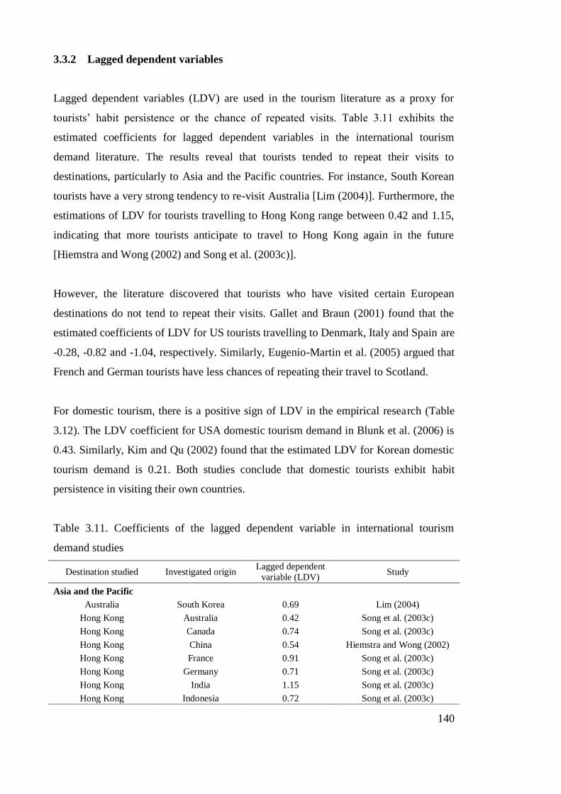
140
3.3.2 Lagged dependent variables
Lagged dependent variables (LDV) are used in the tourism literature as a proxy for
tourists‟ habit persistence or the chance of repeated visits. Table 3.11 exhibits the
estimated coefficients for lagged dependent variables in the international tourism
demand literature. The results reveal that tourists tended to repeat their visits to
destinations, particularly to Asia and the Pacific countries. For instance, South Korean
tourists have a very strong tendency to re-visit Australia [Lim (2004)]. Furthermore, the
estimations of LDV for tourists travelling to Hong Kong range between 0.42 and 1.15,
indicating that more tourists anticipate to travel to Hong Kong again in the future
[Hiemstra and Wong (2002) and Song et al. (2003c)].
However, the literature discovered that tourists who have visited certain European
destinations do not tend to repeat their visits. Gallet and Braun (2001) found that the
estimated coefficients of LDV for US tourists travelling to Denmark, Italy and Spain are
-0.28, -0.82 and -1.04, respectively. Similarly, Eugenio-Martin et al. (2005) argued that
French and German tourists have less chances of repeating their travel to Scotland.
For domestic tourism, there is a positive sign of LDV in the empirical research (Table
3.12). The LDV coefficient for USA domestic tourism demand in Blunk et al. (2006) is
0.43. Similarly, Kim and Qu (2002) found that the estimated LDV for Korean domestic
tourism demand is 0.21. Both studies conclude that domestic tourists exhibit habit
persistence in visiting their own countries.
Table 3.11. Coefficients of the lagged dependent variable in international tourism
demand studies
Destination studied Investigated origin Lagged dependent
variable (LDV) Study
Asia and the Pacific
Australia South Korea 0.69 Lim (2004)
Hong Kong Australia 0.42 Song et al. (2003c)
Hong Kong Canada 0.74 Song et al. (2003c)
Hong Kong China 0.54 Hiemstra and Wong (2002)
Hong Kong France 0.91 Song et al. (2003c)
Hong Kong Germany 0.71 Song et al. (2003c)
Hong Kong India 1.15 Song et al. (2003c)
Hong Kong Indonesia 0.72 Song et al. (2003c)

141
Destination studied Investigated origin Lagged dependent
variable (LDV) Study
Hong Kong Japan 0.67 Hiemstra and Wong (2002)
Hong Kong Japan 0.75 Song et al. (2003c)
Hong Kong Korea 0.99 Song et al. (2003c)
Hong Kong Malaysia 0.47 Song et al. (2003c)
Hong Kong Philippines 0.57 Song et al. (2003c)
Hong Kong Singapore 0.66 Song et al. (2003c)
Hong Kong Taiwan 0.5 Hiemstra and Wong (2002)
Hong Kong Taiwan 0.6 Song et al. (2003c)
Hong Kong Thailand 0.47 Hiemstra and Wong (2002)
Hong Kong Thailand 0.45 Song et al. (2003c)
Hong Kong UK 0.59 Hiemstra and Wong (2002)
Hong Kong UK 1.02 Song et al. (2003c)
Hong Kong USA 0.65 Hiemstra and Wong (2002)
Hong Kong USA 0.58 Song et al. (2003c)
Korea Germany -0.07 Song and Witt (2003)
Korea Japan 1.11 Song and Witt (2003)
Korea UK 0.48 Song and Witt (2003)
Korea USA 0.86 Song and Witt (2003)
Korea USA 0.94 Song and Witt (2003)
Thailand Australia 0.63 Song et al. (2003b)
Thailand Japan 0.59 Song et al. (2003b)
Thailand Korea 0.70 Song et al. (2003b)
Thailand Malaysia 0.73 Song et al. (2003b)
Thailand Singapore 0.82 Song et al. (2003b)
Thailand UK 0.54 Song et al. (2003b)
Thailand USA 0.47 Song et al. (2003b)
Europe
Austria USA -0.62 Gallet and Braun (2001)
British Columbia Japan 0.28 Hui and Yuen (1998)
Denmark Germany 0.75 Song et al. (2003a)
Denmark Norway 0.58 Song et al. (2003a)
Denmark Sweden 0.61 Song et al. (2003a)
Denmark UK 0.49 Song et al. (2003a)
Denmark USA -0.28 Gallet and Braun (2001)
Italy USA -0.82 Gallet and Braun (2001)
Scotland France -0.34 Eugenio-Martin et al. (2005)
Scotland Germany -0.07 Eugenio-Martin et al. (2005)
Scotland USA 0.04 Eugenio-Martin et al. (2005)
Spain USA -1.04 Gallet and Braun (2001)
Spain German 0.21 Garin-Munoz (2007)
Non-sun and non-sea
destinations in Spain German 0.50 Garin-Munoz (2007)
Sun and sea destinations
in Spain German 0.15 Garin-Munoz (2007)
Sweden Denmark 0.23 Salman (2003)
Sweden Finland 0.21 Salman (2003)
Sweden Germany 0.5 Salman (2003)

142
Destination studied Investigated origin Lagged dependent
variable (LDV) Study
Sweden Norway 0.63 Salman (2003)
Sweden UK 0.59 Salman (2003)
Sweden USA 0.74 Salman (2003)
Switzerland USA 1.03 Gallet and Braun (2001)
UK USA -0.08 Gallet and Braun (2001)
Rest of the world
Africa World -0.68 Naude and Saayman (2005)
Note: The elasticity estimations are extracted from the empirical literature of international tourism
demand during 1998 and 2008. The signs of lagged dependent variables indicate the degree of travel
repetition from the previous tourists. Those estimates with positive (negative) sign imply that there is an
increase (decrease) in the number of tourist repetitions.
Table 3.12. Coefficients of lagged dependent variable in domestic tourism demand
Destination studied Lagged dependent variable
(LDV) Source
USA 0.43 Blunk et al. (2006)
Korea
0.21
Kim and Qu (2002)
Note: The elasticity estimations are extracted from the empirical literature of domestic tourism demand.
Thus far, only Blunk et al. (2006) and Kim and Qu (2002) found that lagged dependent variables have
significant impacts on domestic tourism demand. The explanations of the signs are similar to the Table
3.11 above.
3.3.3 Destination preference index (DPI)
Song et al. (2000) introduced a new tourism demand determinant named as the
destination preference index (DPI). It is written as: PREFi = Vi/Vs, where Vi = total
visits to destination i and Vs = total visits to all other competing destinations. If the
index value is high and exceeded one, it suggests that tourists are more likely to prefer
travelling to destination i over the other competing destinations. According to the
authors, the benefit of this index is that it takes account of non-economic factors (i.e.
social, cultural and psychological influences) in tourists‟ decision-making.
Song et al. (2000) examined whether the index has a significant effect on UK demand
for outbound tourism to twelve destinations. Based on the study (Table 3.13), the
destination preference indices for European destinations are high, ranging from 0.79 to
1.1. In contrast, the DPI for USA is 0.12 which is much lower than the DPI for

143
European destinations. This indicates that UK tourists strongly prefer travelling to
Europe rather than to the USA.
Table 3.13. Coefficients of destination preference index in international tourism demand
studies
Destination studied Investigated origin Destination preference
index (DPI) Source
Austria UK 0.85 Song et al. (2000)
Belgium/Luxembourg UK 0.86 Song et al. (2000)
France UK 0.82 Song et al. (2000)
Germany UK 0.94 Song et al. (2000)
Greece UK 1.1 Song et al. (2000)
Irish Republic UK 0.87 Song et al. (2000)
Italy UK 0.81 Song et al. (2000)
Netherlands UK 0.7 Song et al. (2000)
Spain UK 0.79 Song et al. (2000)
Switzerland UK 0.89 Song et al. (2000)
USA UK 0.12 Song et al. (2000)
World UK 0.12 Song et al. (2000)
Note: DPI variable is first constructed by Song et al. (2000) to examine international tourists‟ preferences
in visiting western countries. It takes accounts of non-economic factors (such as social and cultural
factors) in tourists‟ decisions to travel to a destination. According to Song et al. (2000), those coefficients
that exceed one indicate that tourists prefer to travel to the particular destinations.
Since the year 2000, DPI has been introduced in the tourism literature and it is an
alternative variable available to be incorporated into tourism demand studies.
Nevertheless, apart from Song et al. (2000), no other tourism research paper has
considered this variable.
3.3.4 Trade volume or openness to trade
Tourism researchers believe that trade volume or openness to trade between countries of
origin and destination has a certain degree of influence on tourism demand, particularly
for business travel. Kulendran and Wilson (2000) asserted that countries with more
open markets provide opportunities for international trade as well as an expectation of
increasing business tourism demand.
Table 3.14 presents the coefficients of openness to trade that have appeared in the
international tourism demand literature. Based on the Kulendran and Wilson (2000)
study, the estimated coefficients for UK and Japanese demand for business tourism in

144
Australia appear to be 3.95 and 2.6, respectively, which are positive and strongly
elastic. In other words, UK and Japanese business tourists responded to the degree of
openness to trade in Australia.
Table 3.14. Coefficients of trade volume in international tourism demand studies
Destination studied Investigated origin Trade volume or
openness to trade Study
Australia Japan 2.6 Kulendran and Wilson (2000)
Australia New Zealand 0.01 Kulendran and Wilson (2000)
Australia UK 3.95 Kulendran and Wilson (2000)
Australia USA 0.4 Kulendran and Wilson (2000)
New Zealand USA 0.43 Turner and Witt (2001b)
South Korea Germany 0.4 Kim and Song (1998)
South Korea Japan 0.55 Kim and Song (1998)
South Korea UK 0.49 Kim and Song (1998)
South Korea USA 0.55 Kim and Song (1998)
South Korea Germany 0.25 Song and Witt (2003)
South Korea Japan -0.87 Song and Witt (2003)
South Korea UK 0.35 Song and Witt (2003)
Thailand Singapore 0.17 Song et al. (2003b)
Thailand USA 0.18 Song et al. (2003b)
Note: The estimations above are obtained from the empirical literature of international tourism demand
during 1998 and 2008. The main purpose of constructing this summary is to compare the elasticities
across different countries or continents. The estimates vary from one study to another, which could be due
to different models and data used. Refer to Appendix 2.1 for further details.
For Asian countries, the variable has some degree of influence on tourist arrivals to this
region but the effects are not strong (Table 3.14). Kim and Song (1998) and Song and
Witt (2003) examined the effects of trade volume on tourist arrivals to South Korea and
found that the elasticities ranged between -0.87 and 0.55. Apart from that, Song et al.
(2003b) discovered that the trade volume elasticities for tourist arrivals from Singapore
and USA to Thailand are 0.17 and 0.18, respectively.
Hence, referring to the empirical findings, the suggestion is that trade volume or
openness to trade plays a role in determining international tourism demand. However,
most studies found that the estimated elasticities do not exceed one. In other words, the
trade volume impact on tourism demand does not have a major significance.
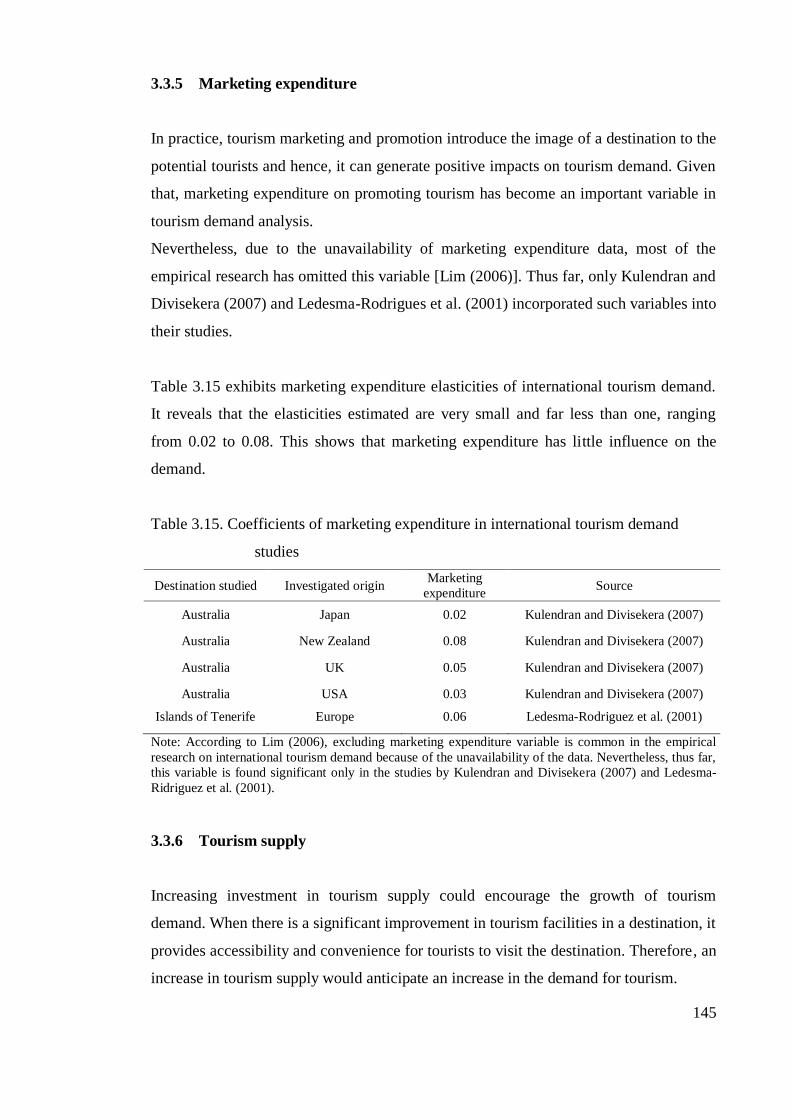
145
3.3.5 Marketing expenditure
In practice, tourism marketing and promotion introduce the image of a destination to the
potential tourists and hence, it can generate positive impacts on tourism demand. Given
that, marketing expenditure on promoting tourism has become an important variable in
tourism demand analysis.
Nevertheless, due to the unavailability of marketing expenditure data, most of the
empirical research has omitted this variable [Lim (2006)]. Thus far, only Kulendran and
Divisekera (2007) and Ledesma-Rodrigues et al. (2001) incorporated such variables into
their studies.
Table 3.15 exhibits marketing expenditure elasticities of international tourism demand.
It reveals that the elasticities estimated are very small and far less than one, ranging
from 0.02 to 0.08. This shows that marketing expenditure has little influence on the
demand.
Table 3.15. Coefficients of marketing expenditure in international tourism demand
studies
Destination studied Investigated origin Marketing
expenditure Source
Australia Japan 0.02 Kulendran and Divisekera (2007)
Australia New Zealand 0.08 Kulendran and Divisekera (2007)
Australia UK 0.05 Kulendran and Divisekera (2007)
Australia USA 0.03 Kulendran and Divisekera (2007)
Islands of Tenerife Europe 0.06 Ledesma-Rodriguez et al. (2001)
Note: According to Lim (2006), excluding marketing expenditure variable is common in the empirical
research on international tourism demand because of the unavailability of the data. Nevertheless, thus far,
this variable is found significant only in the studies by Kulendran and Divisekera (2007) and Ledesma-
Ridriguez et al. (2001).
3.3.6 Tourism supply
Increasing investment in tourism supply could encourage the growth of tourism
demand. When there is a significant improvement in tourism facilities in a destination, it
provides accessibility and convenience for tourists to visit the destination. Therefore, an
increase in tourism supply would anticipate an increase in the demand for tourism.

146
In the international tourism demand literature, the effects of tourism supply have not
been widely examined. The possible reason could be due to the fact that tourism supply
data is not available in most countries. To date, the empirical papers that have
incorporated such a variable are Jimenez (2002), Naude and Saayman (2005), and
Ouerfelli (2008).
Table 3.16 is the summary of tourism supply elasticities that have appeared in the
international tourism demand literature. Naude and Saayman (2005) discovered that a
one percent increase in tourism supply in Africa would lead to 1.11% increase in tourist
arrivals from USA. More recently, Ouerfelli (2008) found that tourism supply
elasticities for French and Italy demand for Tunisia‟s tourism are 3.02 and 2.16,
respectively. However, for developed countries such as Spain, a one percent increase in
tourism supply would only lead to a 0.05% increase in tourist arrivals to Spain. In
summary, an increase in tourism supply in a developing country will have a stronger
and more positive impact on international tourist arrivals in these countries than that in
a developed country.
Table 3.16. Coefficients of tourism supply in international tourism demand studies
Destination studied Investigated origin Tourism supply Source
Africa Europe 0.74 Naude and Saayman (2005)
Africa USA 1.11 Naude and Saayman (2005)
Africa World 0.39 Naude and Saayman (2005)
Spain World 0.05 Jimenez (2002)
Tunisia France 3.02 Ouerfelli (2008)
Tunisia Italy 2.16 Ouerfelli (2008)
Note: The estimations above are obtained from the empirical literature of international tourism demand.
The estimates vary from one study to another, which could be due to different models and data used.
Refer to Appendix 2.1 for further details.
The possible explanation for such results could be that the rise in tourism facilities in
developing countries provides a good opportunity for tourists to visit new and exotic
destinations. In contrast, for developed countries, a growth in tourism supply may not
increase the tourist population remarkably as the tourism products in these countries
have become mature.

147
3.3.7 Working hours
The working hour variable has emerged in the domestic tourism demand literature since
1995 when Hultkrantz (1995) conducted an analysis of domestic tourism demand in
Sweden. According to Hultkrantz, the author assumed that time to work is negatively
correlated with leisure time, as people tend to forego working time for recreation
activities. Based on the study, the working hour coefficients are estimated to be ranged
between -0.51 and -1.59 (Table 3.17).
In the literature, Kim and Qu (2002) supported Hultkrantz‟s assumption. They assessed
whether the number of working hours in Korea has negative impacts on domestic
tourism demand in Korea. The study found that the working hours coefficient is -3.88,
indicating that there was a decline in domestic travel in Korea when the number of
working hours increased.
As the volume of empirical research on domestic tourism demand is little, the
conclusion of whether working hours have impacts on the demand cannot be
generalised. Hence, this area requires more empirical research in the future.
Table 3.17. Coefficients of working hours in domestic tourism demand studies
Destination studied Working hours Source
Korea -3.88 Kim and Qu (2002)
Sweden -1.36(1)
Hultkrantz (1995)
Sweden -0.51(2)
Hultkrantz (1995)
Sweden -1.59(3)
Hultkrantz (1995)
Sweden -1.06(4)
Hultkrantz (1995)
Note: In Hultkrantz‟s study, the estimates are generated based on different dependent variables used,
namely (1) the expenditure on recreation, (2) number of trips to visit friends and relatives, (3) number of
trips to see attractions and events, and (4) number of trips for domestic travel experiences.
3.4 Conclusion
This chapter discussed the demand determinants used in the literature on domestic and
international tourism demand. Several conclusions can be made from the empirical
research:

148
(I) In general, income and tourism prices are the main variables used in modelling
tourism demand.
(II) Income elasticities of domestic tourism demand in developed countries are
higher than that of outbound tourism, whereas the reverse holds in emerging
countries.
(III) In the literature of international tourism demand, the tourism price elasticities
vary across different studies. However, for domestic tourism demand, almost all
empirical research found that the price elasticities are negative and above one.
(IV) Habit persistence and special events have influences on domestic and
international tourism demand.
(V) Apart from the above, other variables namely trade volume, marketing
expenditure, tourist preference and tourism supply can affect international
tourism demand. For domestic tourism demand, working hour variable is found
to be important.
Based on the empirical findings, when there is a significant variation in economic
conditions in developed countries, it is anticipated that domestic tourism demand can be
strongly affected. This thesis focuses on how to sustain domestic tourism demand in
Australia. To do that, we investigate the impacts of household income and tourism price
increases on different types of domestic tourism markets. By doing this, we can evaluate
how different domestic tourists respond to the changes in income and prices.

149
Chapter 4
Australian domestic tourism demand:
Data and seasonality analyses
4.1 Introduction: Australian domestic tourism markets
For Australian residents, travelling is considered as an important household item. In
2006-2007, Australian households consumed about AUD69 billion in recreation and
culture as well as AUD42 billion in hotels, cafes and restaurants. In fact, based on Table
4.1, travelling and tourism products ranked at the top five of the highest value of
household consumption in Australia. Furthermore, during the same period, Australians
spent about AUD52 billion of the Australian produced tourism goods and services,
whereas they spent about AUD18 billion of overseas tourism products3 [Tourism
Satellite Account: 2006-2007 (ABS Cat. No. 5249.0)]. Hence, this indicates that most
Australians travelled domestically more than overseas.
In Australia, domestic tourists can be segmented into domestic overnight and day
visitors. According to Tourism Research Australia, a domestic overnight visitor is a
person who stays one or more nights in one or several destinations during his/her
domestic trips, whereas a domestic day visitor is referred to the person who travels for a
round trip distance of at least 50 kilometres and does not spend a night during the trip.
Each group of tourists can be further segregated into four different purposes of travel;
namely holiday, visiting friends and relatives, business and other.
The data used in this thesis is based on the National Visitor Survey (NVS) which is later
summarised into quarterly reports named as “Travel by Australians”. The survey
measures domestic tourism activity in Australia, including the characteristics and travel
patterns of domestic tourists. The NVS has conducted phone interviews with
approximately 80,000 respondents annually since 1998 and 120,000 since 2005. The
3 The Australian Bureau of Statistics estimated that, in 2006-2007, the average expenditure on domestic
trips is AUD295, which is lower than the average expenditure on outbound trips (AUD4968).
Nevertheless, domestic tourism still plays an important role in the industry because domestic visitors
consumed 73.7% of the Australian tourism products whereas international visitors (which are comprised
of inbound and outbound visitors) consumed 26.3%.

150
respondents are Australian residents aged 15 years and over (See the introduction of the
NVS in the “Travel by Australians” reports).
Table 4.1. Top ten ranking of the most consumed Australian household items, 2006-
2007
Rank Consumption item Value (AUD million)
1 Rent and other dwelling services 96,610
2 Recreations and culture 68,898
3 Food 59,115
4 Hotels, cafes and restaurants 41,810
5 Insurance and other financial products 38,247
6 Other goods and services 36,406
7 Furnishings and household 32,806
8 Operation of vehicles 29,459
9 Health 27,217
10 Clothing and footwear 21,946
Note: The figures are extracted from the Australian National Accounts: National Income, Expenditure
and Product (Cat. no. 5206.0), ABS and it is measured based on current price.
Table 4.2 reveals that most of the domestic overnight visitors travelled for the purposes
of a holiday. In 2008, they stayed approximately 142 million nights for holidays and, on
average, each domestic overnight holiday-maker spent AUD175.43 per night (Table
4.3). Despite that there was a decline of 6.3% in the number of domestic holiday visitor
nights in 2006, the trend reversed as there was a 9.5% increase in 2007. However,
compared with domestic business tourists, the average expenditure per night by a
holiday-maker was about 10% to 36% lower than the average amount spent by a
business traveller.
Tourists who are visiting friends and relatives (VFR) have emerged as a major tourism
market in Australia. Moscardo et al. (2000) found that, apart from visiting friends and
relatives, VFR tourists also engage in activities such as sightseeing or day-trips, visiting
nature destinations, and water-sports. In fact, they discovered that the majority of VFR
tourists were domestic tourists. Based on Table 4.2, this type of tourist ranked second
in terms of the most nights stayed (i.e. 86 million nights in 2008). Nevertheless, the
number of nights spent by VFR tourists has decreased significantly in 2006 and 2008.
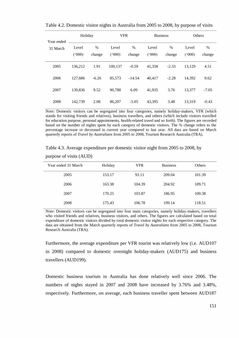
151
Table 4.2. Domestic visitor nights in Australia from 2005 to 2008, by purpose of visits
Year ended
31 March
Holiday VFR Business Others
Level
(„000)
%
change
Level
(„000)
%
change
Level
(„000)
%
change
Level
(„000)
%
change
2005 136,212 1.91 100,137 -0.59 41,358 -2.33 13,129 4.51
2006 127,686 -6.26 85,573 -14.54 40,417 -2.28 14,392 9.62
2007 139,836 9.52 90,788 6.09 41,935 3.76 13,377 -7.05
2008 142,739 2.08 86,207 -5.05 43,395 3.48 13,319 -0.43
Note: Domestic visitors can be segregated into four categories, namely holiday-makers, VFR (which
stands for visiting friends and relatives), business travellers, and others (which include visitors travelled
for education purpose, personal appointments, health-related travel and so forth). The figures are recorded
based on the number of nights spent by each category of domestic visitors. The % change refers to the
percentage increase or decreased in current year compared to last year. All data are based on March
quarterly reports of Travel by Australians from 2005 to 2008, Tourism Research Australia (TRA).
Table 4.3. Average expenditure per domestic visitor night from 2005 to 2008, by
purpose of visits (AUD)
Year ended 31 March Holiday VFR Business Others
2005 153.17 93.11 209.04 101.39
2006 163.38 104.39 204.92 109.71
2007 170.25 103.87 186.95 100.38
2008 175.43 106.78 199.14 118.51
Note: Domestic visitors can be segregated into four main categories, namely holiday-makers, travellers
who visited friends and relatives, business visitors, and others. The figures are calculated based on total
expenditure of domestic visitors divided by total domestic visitor nights for each respective category. The
data are obtained from the March quarterly reports of Travel by Australians from 2005 to 2008, Tourism
Research Australia (TRA).
Furthermore, the average expenditure per VFR tourist was relatively low (i.e. AUD107
in 2008) compared to domestic overnight holiday-makers (AUD175) and business
travellers (AUD199).
Domestic business tourism in Australia has done relatively well since 2006. The
numbers of nights stayed in 2007 and 2008 have increased by 3.76% and 3.48%,
respectively. Furthermore, on average, each business traveller spent between AUD187

152
and AUD209, which surpassed the average expenditure for holiday-makers, VFR and
other visitors (Table 4.3).
Table 4.4 presents a disaggregation of domestic day visitors in Australia by purpose of
visits. Based on the figures, holiday day visitors are the largest share of the overall
domestic day tourism in Australia. In 2008, there were 71 million day visitors who
travelled for holiday purpose, 42 million visitors visited friends and relatives and, 14
million visitors travelled for business trips. In general, Table 4.4 reveals that all
categories of day visitors performed well in 2007 and 2008.
Table 4.4. Domestic day visitors in Australia from 2005 to 2008, by purpose of visits
Year ended
31 March
Holiday VFR Business Others
Level
(„000)
%
change
Level
(„000)
%
change
Level
(„000)
%
change
Level
(„000) % change
2005 68,649 -3.82 37,625 -6.95 11,758 -0.03 13,346 -11.94
2006 69,869 1.78 36,679 -2.51 11,513 -2.08 12,552 -5.95
2007 71,124 1.80 40,125 9.40 12,190 5.88 14,193 13.07
2008 71,579 0.64 42,448 5.79 14,091 15.59 14,843 4.58
Note: The figures are extracted from the March quarterly reports of Travel by Australians from 2005 to
2008, Tourism Research Australia (TRA). According to TRA, domestic day visitors can be disaggregated
into four purposes of visits, namely holiday, visiting friends and relatives (VFR), business-related
purposes, and others (include those visitors who travelled for education, health reasons, and so forth). %
change refers to the percentage increase or decreased in current year compared to last year.
Nevertheless, in terms of comparing the average expenditure by domestic overnight and
day visitors, there was a remarkable difference in the spending behaviour of both groups
of visitors. For instance, an overnight holiday tourist could spend between AUD656 and
AUD763 whereas the average expenditure per holiday day visitor ranges from AUD98
to AUD116 (Table 4.5). Similarly, based on the figures in Table 4.5, a VFR overnight
visitor consumed an average of AUD363 whereas only AUD70 for a VFR day visitor.
Hence, this shows that domestic overnight visitors have a higher willingness to spend
than domestic day visitors.
Furthermore, a recent finding in the domestic tourism demand literature showed that
travel decisions by domestic tourists were influenced by whether the destinations were

153
intrastate or interstate [Huybers (2003)]. A possible reason for such decisions is that the
costs of travelling to interstate or intrastate destinations are relatively different. Hence,
based on the study, domestic tourism in Australia can be segregated into two groups,
namely interstate and intrastate tourism.
Tourism Research Australia distinguishes intrastate and interstate tourism differently.
An intrastate tourist visits a location in the State or Territory in which they reside,
whereas an interstate tourist visits a State or Territory other than that in which they
reside. However, when a same person travel different regions in a single trip, then the
respondent is counted as a single visitor in each region. For example, consider an
Australian from Newcastle travels on a 12 night trip and the person spends 2 nights in
Sydney, 2 nights in Canberra, 4 nights in Melbourne, 2 nights in Benalla and 2 nights in
Wangaratta. Hence, at the State/Territory level, the respondent would be counted as an
interstate visitor to Victoria and the ACT, respectively, as well as an intrastate visitor to
NSW (See the glossary of terms in the “Travel by Australians” reports). The intrastate
and interstate tourism data mainly focuses on domestic visitors and do not include
international tourists.
For the year ended 31 March 2008, the numbers of intrastate and interstate tourists in
Australia were 49.9 million and 24.6 million, respectively [Travel by Australians:
March Quarter 2008 (June 2008)]. Compared to the year ended 31 March 2006, the
numbers of intrastate and interstate visitors in Australia had increased by 3.2 and 1.6
million visitors, respectively [Travel by Australians: March Quarter 2008 (June 2008)
and Travel by Australians: March Quarter 2006 (September 2006)]. Furthermore, for
the year ended 31 March 2008, the total expenditure by intrastate and interstate
overnight visitors was AUD36 billion, which is about 13% more than the total
expenditure in 2006.
Interstate visitors are relatively different from intrastate visitors in terms of the length of
trips and travel expenditure. For the year ended 31 March 2008, the number of night
stays per interstate traveller in Australia was 5.3 nights, whereas it was 3.2 nights for
every intrastate visitor. In terms of expenditure, the average spending per intrastate and
interstate visitor was AUD365 and AUD741, respectively.

154
Table 4.5. Average expenditure per domestic overnight and day visitors from 2005 to
2008, by purpose of visits (AUD)
Year ended
31 March
Holiday VFR Business Others
Overnight Day Overnight Day Overnight Day Overnight Day
2005 656.38 98.98 345.81 60.68 625.26 93.25 351.33 99.05
2006 693.86 107.93 370.08 68.68 620.44 97.96 412.16 101.71
2007 738.68 112.04 371.75 72.85 569.22 96.16 363.31 102.21
2008 763.27 115.60 362.78 76.37 603.85 90.91 428.91 106.90
Note: Each respective domestic overnight and day visitors can be segregated into four categories, namely
holiday-makers, travellers who visited friends and relatives (VFR), business visitors and others (include
visitors who travelled for education, health and so forth). The figures calculate the amount of monies
spent by each domestic overnight and day visitors, respectively. All data are obtained from the March
quarterly reports of Travel by Australians from 2005 to 2008, Tourism Research Australia (TRA).
Expenditure by intrastate and interstate visitors is an important source of revenue for the
tourism industry in each Australia State/Territory. According to Figure 4.1, the
expenditure by intrastate visitors exceeded the spending by international visitors in New
South Wales, Queensland and Western Australia. Moreover, the expenditure by
interstate visitors surpassed the amount of spending by international visitors in Victoria,
South Australia, Tasmania, Northern Territory and Australian Capital Territory. West
and Gamage (2001) studied the economic impacts of tourism on the Victorian economy
and they discovered that interstate tourism contributes the greatest amount of gross state
product and employment to the Victorian economy in Australia compared to other types
of tourists.
Furthermore, because domestic tourists have different spending habits, the segregation
of the domestic tourism market depends on the types of activities that the tourists
participated in. For instance, about 21 million domestic tourists have engaged in cultural
and heritage tourism in Australia in 2007 and they have spent a total of AUD12 billion
during the year [Cultural and Heritage Tourism in Australia 2007 (2008)]. Another type
of domestic tourism is called nature-based tourism. In 2007, there were 29.38 million
domestic nature-based tourists who have spent AUD15 billion in this type of tourism.
Particularly for domestic overnight nature visitors, the average expenditure per person
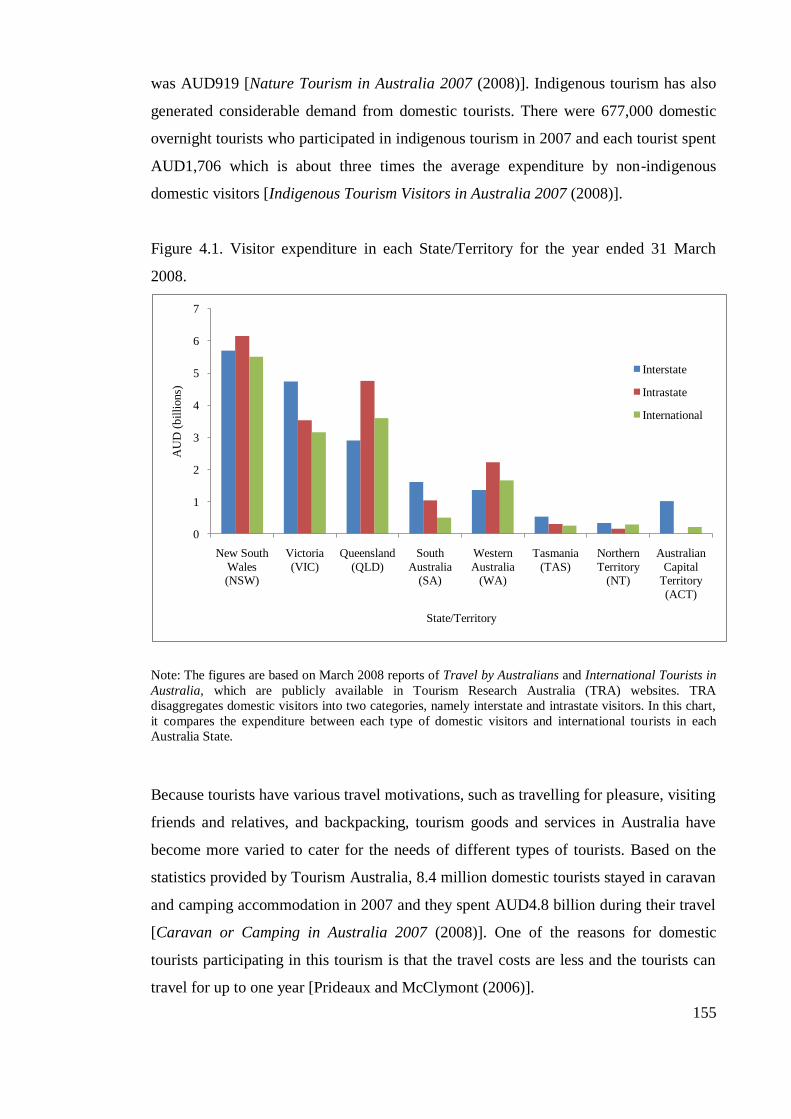
155
was AUD919 [Nature Tourism in Australia 2007 (2008)]. Indigenous tourism has also
generated considerable demand from domestic tourists. There were 677,000 domestic
overnight tourists who participated in indigenous tourism in 2007 and each tourist spent
AUD1,706 which is about three times the average expenditure by non-indigenous
domestic visitors [Indigenous Tourism Visitors in Australia 2007 (2008)].
Figure 4.1. Visitor expenditure in each State/Territory for the year ended 31 March
2008.
Note: The figures are based on March 2008 reports of Travel by Australians and International Tourists in
Australia, which are publicly available in Tourism Research Australia (TRA) websites. TRA
disaggregates domestic visitors into two categories, namely interstate and intrastate visitors. In this chart,
it compares the expenditure between each type of domestic visitors and international tourists in each
Australia State.
Because tourists have various travel motivations, such as travelling for pleasure, visiting
friends and relatives, and backpacking, tourism goods and services in Australia have
become more varied to cater for the needs of different types of tourists. Based on the
statistics provided by Tourism Australia, 8.4 million domestic tourists stayed in caravan
and camping accommodation in 2007 and they spent AUD4.8 billion during their travel
[Caravan or Camping in Australia 2007 (2008)]. One of the reasons for domestic
tourists participating in this tourism is that the travel costs are less and the tourists can
travel for up to one year [Prideaux and McClymont (2006)].
0
1
2
3
4
5
6
7
New South
Wales (NSW)
Victoria
(VIC)
Queensland
(QLD)
South
Australia (SA)
Western
Australia (WA)
Tasmania
(TAS)
Northern
Territory (NT)
Australian
Capital Territory
(ACT)
AU
D (
bil
lions)
State/Territory
Interstate
Intrastate
International

156
In addition, Australians who prefer to stay in backpacker accommodation have
increased in recent years. The number of nights that domestic tourists stayed in
backpacker accommodation increased from 1.3 million in 2005 to 1.7 million nights in
2007. Furthermore, the average spending by these tourists was AUD831 per person,
which is about 41% more than those domestic tourists who did not stay in backpacker
accommodation [Backpacker Accommodation in Australia 2007 (2008)]. The increasing
popularity of backpacking among domestic tourists is because the tourists can save on
accommodation and spend their money for sightseeing tours and adventurous activities
[Mohsin and Ryan (2003)].
4.2 Domestic tourism performance by state
From the discussion above, it is evident that domestic tourism is an important tourism
business in Australia. In fact, within domestic tourism, overnight travel is the most
important market segment in the industry. Given this, the current research is motivated
to conduct trend and seasonality analyses on domestic overnight tourism in eight
Australian States and Territories (the major and populated ones only). The main
intention is to obtain a better understanding of domestic overnight tourism in every
State. Furthermore, as domestic overnight tourists can be segregated into various types
of visitors, such as holiday-makers and business tourists, key overnight tourism markets
in each State are identified and seasonality in travel is explored. By doing this, it should
be able to support development of tourism policies to sustain domestic overnight
tourism in each State.
For this thesis, eight types of disaggregated domestic overnight tourist data, which are
obtained from Travel by Australians (1999 – 2007), are analysed. They are the numbers
of: (1) interstate overnight visitors; (2) intrastate overnight visitors; (3) interstate visitor
nights; (4) intrastate visitor nights; (5) holiday visitor nights; (6) business visitor nights;
(7) visitor nights by domestic travellers for visiting friends and relatives; and (8) visitor
nights by domestic travellers for other visit purposes such as education and working
holidays. These data are available on a quarterly basis from 1999 to 2007.
157
4.2.1 Australian Capital Territory (ACT)
Australian Capital Territory (ACT) hosts the Parliament of Australia and Canberra is
the capital city for both ACT and Australia. The city offers a range of national
institutions for visitors, such as the National Gallery of Australia, Parliament House,
National Film and Sound Archive, and Australian War Memorial (refer to The National
Capital Authority website4
). Furthermore, Canberra is surrounded by hills and
bushlands, with 34 reserves being collectively known as „Canberra Nature Park‟. These
include Black Mountain, Mount Ainslie, Mount Majura, Mount Mugga, O‟Connor
Ridge, Bruce Ridge, Aranda Bushland, Mount Painter, The Pinnacle, Lyneham Ridge,
Oakey Hill, Mount Taylor, Issaacs Ridge, Mount Stromlo, Mount Arawang, Neighbour
Hill, Wnaniassa Hill, and Narrabundah Hill5. As the parks offer easily accessible
facilities, visitors are encouraged to participate in numerous tourist activities such as
camping, hiking, fishing, swimming and horse-riding. Other natural areas, such as the
Brindabella Ranges, are easily accessed from Canberra.
Domestic tourism in the ACT mostly attracts visitors who are visiting friends and
relatives (VFR), or are on business trips (BUS). Based on Table 4.6, on average, the
total nights spent by VFR tourists in each quarter were 594,444. For business visitors,
the average number of visitor nights for each quarter was 366,139. During 1999 and
2007, the maximum amount of nights spent in ACT by VFR and BUS travellers were
912,000 and 598,000, respectively.
Nonetheless, VFR visitor nights can be highly variable, with the number surging in
2003 [See Figure 4.2 (Panel B)]. This could be due to the outbreak of SARS virus that
encouraged more Australians to visit their friends and family in ACT rather than to
travel overseas. In contrast, the trend for the BUS visitor night data is rather constant
[Figure 4.2 (Panel C)].
4 http://www/nationalcapital.gov.au/visiting/overview.asp
5 Refer to “Get out there: A guide to the Australian Capital Territory‟s parks and open space system”,
http://www.tams.act.gov.au/play/parks_forrests_and_reserves/get_out_there

158
Table 4.6. Descriptive statistics of domestic visitor nights („000) in ACT for quarterly
data from 1999 to 2007
HOL VFR BUS OTH
Mean 361 594.4 366.1 83.2
Maximum 762 912 598 269
Minimum 210 415 185 12
Std. Dev. 112.6 130.5 111.2 54.5
C.V. (%) 31.2 22 30.4 65.5
Note: HOL = holiday visitors; VFR = visitors of friends and relatives; BUS = business visitors; and OTH
= other types of visitors (i.e. working-related trips, education and health purposes). For ACT, the
quarterly data on interstate and intrastate tourism demand are not reliable and hence, this thesis omits a
discussion about such data. Std. Dev. = standard deviation. C.V. = Coefficient of variation. Source:
Travel by Australians
Holiday-makers (HOL) are also considered as an important tourist market sector in
ACT. Even thought HOL visitors spent fewer nights in ACT (an average of 361, 000
nights per quarter during 1999 to 2007), the maximum number is higher than that for
BUS visitors (Table 4.6). Regarding the variations of HOL and VFR visitor night data,
the HOL visitor nights has higher coefficient of variation than its counterparts.
Between 1999 and 2007, HOL and OTH visitor night data display a downward trend
[Figure 4.2 (Panels A and D)]. Furthermore, there were two sharp declines in the
number of HOL visitor nights. The first fall occurred in the middle year of 2000, but
when the 9/11 terrorist attacks happened, it gradually increased in 2001 and early 2002.
The second drop in HOL visitor nights took place in the middle of 2002. However,
since then, the visitor night data have remained stable.
Except for BUS, all types of visitors stayed the most nights during January to March
(Table 4.7). A possible reason is that this period is the major holiday season for schools
and universities in Australia, and that has encouraged visitors to spend longer nights in
ACT. On the basis of average number of visitor nights, VFR visitor is the most
important domestic tourist market in ACT in each quarter.

159
Figure 4.2. Visitor nights by purpose of visits in ACT
Panel (A): Holiday (HOL)
Panel (B): Visiting friends and relatives (VFR)
Panel (C): Business (BUS)
0
100
200
300
400
500
600
700
800
900
Mar
-99
Sep
-99
Mar
-00
Sep
-00
Mar
-01
Sep
-01
Mar
-02
Sep
-02
Mar
-03
Sep
-03
Mar
-04
Sep
-04
Mar
-05
Sep
-05
Mar
-06
Sep
-06
Mar
-07
Sep
-07
'000
HOL
Linear
(HOL)
0
100
200
300
400
500
600
700
800
900
1,000
Mar
-99
Sep
-99
Mar
-00
Sep
-00
Mar
-01
Sep
-01
Mar
-02
Sep
-02
Mar
-03
Sep
-03
Mar
-04
Sep
-04
Mar
-05
Sep
-05
Mar
-06
Sep
-06
Mar
-07
Sep
-07
'000
VFR
Linear
(VFR)
0
100
200
300
400
500
600
700
Mar
-99
Sep
-99
Mar
-00
Sep
-00
Mar
-01
Sep
-01
Mar
-02
Sep
-02
Mar
-03
Sep
-03
Mar
-04
Sep
-04
Mar
-05
Sep
-05
Mar
-06
Sep
-06
Mar
-07
Sep
-07
'000
BUS
Linear
(BUS)

160
Panel (D): Others (OTH)
Note: The figures above are computed using quarterly time-series data which are extracted from Travel by
Australians, published by Tourism Research Australia (TRA). The linear line in each panel is generated
using a trend regression, which is written as follows: 𝑦𝑡 = 𝛼1 + 𝛼2𝑡 + 𝜀𝑡 , where y = domestic tourism
data, t = time trend, α1,2 = estimated coefficients, ε = error term. The main intention of estimating the
linear trend is to observe the long-term trend of the data.
Table 4.7. Visitor nights („000) in ACT by purpose of visits in each quarter
Quarter HOL VFR BUS OTH
January – March 382.7 656.6 304.6 109.2
April – June 376.3 569.7 383.7 79.4
July – September 324.8 537.4 381.4 69.7
October - December 360.2 614.1 394.9 74.3
Note: HOL = holiday visitor nights, VFR = visitor nights by visiting friends and relatives, BUS =
business visitor nights, OTH = visitor nights by other types of travellers. The figures above are the
average value of domestic tourism demand in each quarter. They are estimated using an econometric
regression with seasonal dummy variables, as follows: 𝑦𝑡 = 𝛼1𝑆𝐷1𝑡 + 𝛼2𝑆𝐷2𝑡 + 𝛼3𝑆𝐷3𝑡 + 𝛼4𝑆𝐷4𝑡 + 𝜀𝑡 , where y = domestic tourism data, t = time, αi = estimated coefficients, SD1 = seasonal dummy for 1
st
quarter (January – March), SD2 = seasonal dummy for 2nd
quarter (April – June), SD3 = seasonal dummy
for 3rd
quarter (July – September), SD4 = seasonal dummy for 4th quarter (October – December), ε = error
terms. The time-series data used are based on the Travel by Australians from 1999Q1 to 2007Q4.
4.2.2 New South Wales (NSW)
New South Wales (NSW) is the oldest and second most densely populated Australian
State after Victoria. In 2007, the population had increased to nearly 6.9 million people6.
6 Refer to http://en.wikipedia.org/wiki/New_south_wales
0
50
100
150
200
250
300
Mar
-99
Sep
-99
Mar
-00
Sep
-00
Mar
-01
Sep
-01
Mar
-02
Sep
-02
Mar
-03
Sep
-03
Mar
-04
Sep
-04
Mar
-05
Sep
-05
Mar
-06
Sep
-06
Mar
-07
Sep
-07
'000
OTH
Linear
(OTH)
161
Intrastate travel has been divided into short-trip and regional destinations7. Short-trip
destinations such as the Blue Mountains, the Hunter Valley, Port Stephens and the
Central Coast, are within 2.5 hours drive from Sydney. The uniqueness of these
destinations is that they are well-known for their winery, spa, heritage and nature-
seeking tourism. Regional destinations in NSW include the North Coast, South Coast,
Snowy Mountains, Lord Howe Island and the country- side in general. These regions
offer farm-stay experience, hiking and skiing, water-sport activities and Aboriginal
culture tourism. Furthermore, Sydney is not only famous for its Harbour Bridge, Opera
House and Darling Harbour, it is also popular for its parks and beaches, such as Royal
National Park, Bondi and Manly Beaches. The city has hosted several international
sporting and political events such as the 2000 Summer Olympics, 2003 Rugby World
Cup and 21st APEC Economies for APEC Australia 2007.
Holiday visitors (HOL) and travellers who were visiting friends and relatives (VFR) are
the main domestic market segments in NSW. HOL visitors spent more nights than VFR,
business travellers (BUS) and other types of domestic visitors (OTH). On average, they
stayed ten million nights per quarter (Table 4.8) with a maximum of about 16 million
nights from 1999 to 2007. The equivalent data for VFR tourists were 7.6 and ten million
nights, respectively, making VFR the second most important domestic tourist market in
NSW.
Both HOL and VFR visitor night data display significant seasonal variations [Figure 4.3
(Panels A and B)]. In fact, the peak (low) season for these visitors travelling to or within
NSW falls in the beginning (middle) of the calendar year. However, the HOL data have
shown a declining trend between 1999 and 2007, while VFR data have a constant trend.
BUS and OTH visitors in NSW spent fewer total nights than HOL and VFR, staying on
average about three and one millions nights, respectively (Table 4.8). However, there is
a continuous decline in the BUS visitor nights in NSW [Figure 4.3 (Panel C)], and that
would be a concern to NSW‟s tourism stakeholders in the light of sustaining business
7 Refer to the online brochure “Sydney and New South Wales, Australia” by Tourism New South Wales
(http://www.visitnsw.com/Travellers_tool_kit_p2233.aspx)

162
tourism in NSW. For OTH visitor nights, the trend is rather stable [Figure 4.3 (Panel
D)].
Table 4.8. Descriptive statistics of domestic tourist markets in NSW („000)
Note: HOL = holiday visitor nights; VFR = number of night visited by visitors of friends and relatives;
BUS = business visitor nights; OTH = number of visitor nights by other types of visitors (i.e. working-
related trips, education and health purposes); NV = interstate visitor nights; NVI = intrastate visitor
nights; OV = interstate overnight visitors; and OVI = intrastate overnight visitors. Max. = maximum; Min
= minimum; S.D. = standard deviation; and C.V. = Coefficient of variation. Source: Quarterly data (1999-
2007) from the quarterly reports of Travel by Australians.
Figure 4.3. Numbers of visitor nights by purpose of visits and numbers of interstate and
intrastate visitors in NSW
Panel (A): Holiday visitor nights (HOL)
0
2,000
4,000
6,000
8,000
10,000
12,000
14,000
16,000
18,000
Mar
-99
No
v-9
9
Jul-
00
Mar
-01
No
v-0
1
Jul-
02
Mar
-03
No
v-0
3
Jul-
04
Mar
-05
No
v-0
5
Jul-
06
Mar
-07
No
v-0
7
'000
HOL
Linear (HOL)
HOL VFR BUS OTH NV NVI OV OVI
Mean 10233.7 7601.8 3043.6 1025.3 8458 13717.8 1983 4450.8
Max. 15891 10165 4327 1587 11031 18995 2285 5092
Min. 7386 5416 2317 706 6509 10179 1745 3595
S.D. 2669.7 1046.2 433.7 209.1 1336 2267.3 137.8 392.2
C.V. (%) 26.088 13.8 14.2 20.4 15.8 16.5 7 8.8

163
Panel (B): Visitor nights by visiting friends and relatives (VFR)
Panel (C): Business visitor nights (BUS)
Panel (D): Visitor nights by other types of travellers (OTH)
0
2,000
4,000
6,000
8,000
10,000
12,000
Mar
-99
No
v-9
9
Jul-
00
Mar
-01
No
v-0
1
Jul-
02
Mar
-03
No
v-0
3
Jul-
04
Mar
-05
No
v-0
5
Jul-
06
Mar
-07
No
v-0
7
'00
0VFR
Linear (VFR)
0
500
1,000
1,500
2,000
2,500
3,000
3,500
4,000
4,500
5,000
Mar
-99
No
v-9
9
Jul-
00
Mar
-01
No
v-0
1
Jul-
02
Mar
-03
No
v-0
3
Jul-
04
Mar
-05
No
v-0
5
Jul-
06
Mar
-07
No
v-0
7
'000
BUS
Linear (BUS)
0
200
400
600
800
1,000
1,200
1,400
1,600
1,800
Mar
-99
No
v-9
9
Jul-
00
Mar
-01
No
v-0
1
Jul-
02
Mar
-03
No
v-0
3
Jul-
04
Mar
-05
No
v-0
5
Jul-
06
Mar
-07
No
v-0
7
'000
OTH
Linear (OTH)
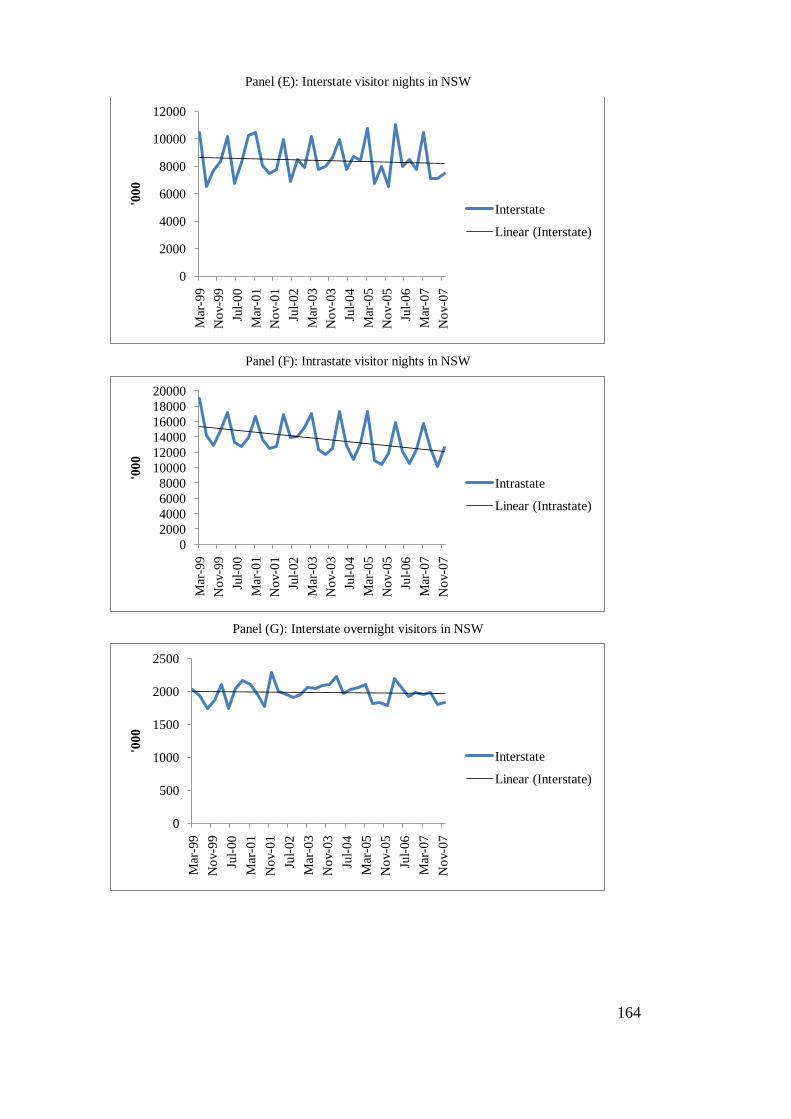
164
Panel (E): Interstate visitor nights in NSW
Panel (F): Intrastate visitor nights in NSW
Panel (G): Interstate overnight visitors in NSW
0
2000
4000
6000
8000
10000
12000
Mar
-99
No
v-9
9
Jul-
00
Mar
-01
No
v-0
1
Jul-
02
Mar
-03
No
v-0
3
Jul-
04
Mar
-05
No
v-0
5
Jul-
06
Mar
-07
No
v-0
7
'000
Interstate
Linear (Interstate)
0
2000
4000
6000
8000
10000
12000
14000
16000
18000
20000
Mar
-99
No
v-9
9
Jul-
00
Mar
-01
No
v-0
1
Jul-
02
Mar
-03
No
v-0
3
Jul-
04
Mar
-05
No
v-0
5
Jul-
06
Mar
-07
No
v-0
7
'000
Intrastate
Linear (Intrastate)
0
500
1000
1500
2000
2500
Mar
-99
No
v-9
9
Jul-
00
Mar
-01
No
v-0
1
Jul-
02
Mar
-03
No
v-0
3
Jul-
04
Mar
-05
No
v-0
5
Jul-
06
Mar
-07
No
v-0
7
'000
Interstate
Linear (Interstate)

165
Panel (H): Intrastate overnight visitors in NSW
Note: The figures above are computed using quarterly time-series data which are extracted from Travel by
Australians, published by Tourism Research Australia (TRA). The linear line in each panel is generated
using a trend regression, which is written as follows: 𝑦𝑡 = 𝛼1 + 𝛼2𝑡 + 𝜀𝑡 , where y = domestic tourism
data, t = time trend, α1,2 = estimated coefficients, ε = error term. The main intention of estimating the
linear trend is to observe the long-term trend of the data.
Nevertheless, the degrees of variation of data for both BUS and OTH visitor night data
are different from each other. On one hand, the BUS visitor night data do not vary as
much as the HOL visitor night data. In fact, the standard deviation of BUS is 433,674
nights, while the standard deviation of HOL is three million nights (Table 4.8). On the
other hand, the coefficient of variation for OTH visitor night data is higher than VFR
visitor nights, implying that the former data is more volatile (Table 4.8).
Another interesting characteristic of NSW tourism is that intrastate visitors spent more
nights in NSW than interstate visitors. Table 4.8 reveals that, on average, 4.5 million
intrastate visitors stayed about 14 million nights, while two million interstate visitors
stayed 8.4 million nights. This shows that the majority of the domestic tourists in NSW
are intrastate travellers and that could relate to the popular short-distance destinations in
NSW which attract the residents in NSW to travel within their own state. Clearly, there
are more visitor nights per interstate visitor (4.3 nights) than intrastate (3.1 nights)
visitor.
The data on domestic interstate and intrastate tourism in NSW reveal several
characteristics. The visitor night data show very strong seasonality [Figure 4.3 (Panels E
- H)]. In fact, the most nights spent by interstate and intrastate visitors occurred during
0
1000
2000
3000
4000
5000
6000
Mar
-99
No
v-9
9
Jul-
00
Mar
-01
No
v-0
1
Jul-
02
Mar
-03
No
v-0
3
Jul-
04
Mar
-05
No
v-0
5
Jul-
06
Mar
-07
No
v-0
7
'000
Intrastate
Linear (Intrastate)

166
the fourth quarter of the year, which was due to the holiday season at the end of the
year. Despite that, there was a downward trend in intrastate tourism demand data since
the beginning of 2005. This could be due to the rising household income that has
encouraged NSW residents to travel overseas or interstate. Apart from that, the numbers
of interstate overnight visitors and visitor nights in 2005 are recorded the lowest.
The average visitor nights stayed in NSW by different types of travellers in each
quarter. Table 4.9 reveals that, while quarterly differences were much greater for HOL
than VFR tourists, both groups spent the most nights between January and March,
where they stayed 15 and nine millions nights, respectively, in the period. Similarly,
interstate and intrastate overnight visitors travelled mostly between January and March.
In fact, about five millions intrastate visitors stayed 17 millions nights in NSW, whereas
two million interstate visitors spent ten millions nights (Table 4.9). However, the peak
travel seasons for BUS and OTH visitors were from July to September and from
October to December, respectively.
Table 4.9. Average domestic tourism demand in NSW in each quarter of the year („000)
Quarter HOL VFR BUS OTH NV NVI OV OVI
Jan –Mar 14638.6 8829.2 2867.4 909 10380.9 16992 2085.7 4774.7
Apr – Jun 8884 7108.7 2914 1102.3 7294.9 12859.3 1937.3 4449.7
Jul – Sep 8420.4 6732.1 3342.1 968.3 8021.7 11782.9 1909.1 4158.1
Oct – Dec 8991.9 7737.1 3050.8 1121.6 8124.5 13383.5 1997.9 4480.8
Note: HOL = holiday visitor nights; VFR = number of night visited by visitors of friends and relatives;
BUS = business visitor nights; OTH = number of visitor nights by other types of visitors (i.e. working-
related trips, education and health purposes); NV = interstate visitor nights; NVI = intrastate visitor
nights; OV = interstate overnight visitors; and OVI = intrastate overnight visitors. The figures above are
the average value of domestic tourism demand in each quarter. They are estimated using an econometric
regression with seasonal dummy variables, as follows: 𝑦𝑡 = 𝛼1𝑆𝐷1𝑡 + 𝛼2𝑆𝐷2𝑡 + 𝛼3𝑆𝐷3𝑡 + 𝛼4𝑆𝐷4𝑡 + 𝜀𝑡 , where y = domestic tourism data, t = time, αi = estimated coefficients, SD1 = seasonal dummy for 1
st
quarter (January – March), SD2 = seasonal dummy for 2nd
quarter (April – June), SD3 = seasonal dummy
for 3rd
quarter (July – September), SD4 = seasonal dummy for 4th quarter (October – December), ε = error
terms. The time-series data used are based on the Travel by Australians from 1999Q1 to 2007Q4.
Overall, two conclusions can be made from the above discussions. First, most of
domestic visitors travelled to NSW at the beginning of the year. Second, holiday-
makers, VFR and intrastate overnight visitors are the most important markets for
domestic tourism businesses in NSW, based only on number of visitor nights.

167
4.2.3 Northern Territory (NT)
Northern Territory (NT) is the third largest but least populated major territory in
Australia8. Nonetheless, the state is rich in Aboriginal culture and art, and native
wildlife. It also has a total of 52 national parks and nature conservation reserves9, which
contain the world famous and spectacular natural rock formations, namely Uluru (Ayers
Rock) and Kata Tjuta (The Olgas). Hence, tourism in NT offers Aboriginal tours and
nature-adventure activities to visitors, where the tourists can learn about Aboriginal
lifestyles and relax by fishing, camel-riding and trekking.
The main domestic tourist markets in NT are holiday-makers (HOL) and business
visitors (BUS). According to Table 4.8, the average and maximum holiday visitor nights
in each quarter for 1999 to 2007 were 806,222 and two million nights, respectively. The
equivalent data for BUS tourists were about 420,194 and one million nights. However,
HOL data exhibit higher coefficient of variation than BUS data, indicating that the
former are more volatile (Table 4.10).
Table 4.10. Descriptive statistics of domestic tourist markets in NT („000)
Note: HOL = holiday visitor nights; VFR = number of night visited by visitors of friends and relatives;
BUS = business visitor nights; OTH = number of visitor nights by other types of visitors (i.e. working-
related trips, education and health purposes); NV = interstate visitor nights; NVI = intrastate visitor
nights; OV = interstate overnight visitors; and OVI = intrastate overnight visitors. Max. = maximum; Min
= minimum; S.D. = standard deviation; and C.V. = Coefficient of variation. Source: Quarterly data (1999-
2007) from the quarterly reports of Travel by Australians.
VFR and OTH visitors stayed fewer nights in NT compared to HOL and BUS tourists.
Based on Table 4.10, the mean visitor nights by VFR and OTH during 1999 and 2007
were 291,750 and 67,444 nights, respectively. Moreover, OTH tourists spent as few as
9,000 nights compared to VFR tourists (59,000 nights). With regard to the degree of
8 Refer to http://en.wikipedia.org/wiki/States_and_territories_of_Australia
9 Refer to http://en.travelnt.com/experience/nature.aspx
HOL VFR BUS OTH NV NVI OV OVI
Mean 806.2 291.8 420.2 67.4 1364.9 358.8 147.9 113.4
Max. 1717 588 1013 282 2830 707 280 163
Min. 174 59 178 9 477 177 58 77
S.D. 476.3 146.5 162.5 53.8 700.7 104.6 65.1 24.7
C.V. (%) 59.1 50.2 38.7 79.8 51.3 29.2 44 21.8

168
volatility of the data, OTH visitor night data demonstrates the highest coefficient of
variation.
Figure 4.4 reveals the historical trends of visitor nights by four types of visitors (namely
HOL, BUS, VFR, and OTH). Accordingly, HOL and VFR visitor night data present
significant seasonal patterns, but in 2003, there was a low record of the visitor night
data in the year. Similarly, BUS visitor night data in 2003 declined significantly
compared to 2002. An underlying reason could be the collapse of the Ansett Airline
which ceased domestic flights in 2002 and caused the total number of domestic flight to
decline significantly at that time. Overall, there is an increasing trend for HOL and VFR
visitor night data but not for the BUS and OTH data.
Figure 4.4. Numbers of visitor nights by purpose of visits and numbers of interstate and
intrastate visitors in NT
Panel (A): Holiday visitor nights (HOL)
Panel (B): Visitor nights by visiting friends and relatives (VFR)
0
500
1,000
1,500
2,000
Mar
-99
No
v-9
9
Jul-
00
Mar
-01
No
v-0
1
Jul-
02
Mar
-03
No
v-0
3
Jul-
04
Mar
-05
No
v-0
5
Jul-
06
Mar
-07
No
v-0
7
'000
HOL
Linear (HOL)
0
100
200
300
400
500
600
700
Mar
-99
Oct
-99
May
-00
Dec
-00
Jul-
01
Feb
-02
Sep
-02
Apr-
03
No
v-0
3
Jun-0
4
Jan-0
5
Aug-0
5
Mar
-06
Oct
-06
May
-07
Dec
-07
'000
VFR
Linear (VFR)

169
Panel (C): Business visitor nights (BUS)
Panel (D): Visitor nights by other types of travellers (OTH)
Panel (E): Interstate visitor nights in NT
0
200
400
600
800
1,000
1,200
Mar
-99
No
v-9
9
Jul-
00
Mar
-01
No
v-0
1
Jul-
02
Mar
-03
No
v-0
3
Jul-
04
Mar
-05
No
v-0
5
Jul-
06
Mar
-07
No
v-0
7
'000
BUS
Linear (BUS)
0
50
100
150
200
250
300
Mar
-99
Oct
-99
May
-00
Dec
-00
Jul-
01
Feb
-02
Sep
-02
Apr-
03
No
v-0
3
Jun-0
4
Jan-0
5
Aug-0
5
Mar
-06
Oct
-06
May
-07
Dec
-07
'000
OTH
Linear (OTH)
0
500
1000
1500
2000
2500
3000
Mar
-99
No
v-9
9
Jul-
00
Mar
-01
No
v-0
1
Jul-
02
Mar
-03
No
v-0
3
Jul-
04
Mar
-05
No
v-0
5
Jul-
06
Mar
-07
No
v-0
7
'000
Interstate
Linear (Interstate)

170
Panel (F): Intrastate visitor nights in NT
Panel (G): Interstate visitors in NT
Panel (H): Intrastate visitors in NT
Note: The figures above are computed using quarterly time-series data which are extracted from Travel by
Australians, published by Tourism Research Australia (TRA). The linear line in each panel is generated
using a trend regression, which is written as follows: 𝑦𝑡 = 𝛼1 + 𝛼2𝑡 + 𝜀𝑡 , where y = domestic tourism
data, t = time trend, α1,2 = estimated coefficients, ε = error term. The main intention of estimating the
linear trend is to observe the long-term trend of the data.
0
100
200
300
400
500
600
700
800
Mar
-99
No
v-9
9
Jul-
00
Mar
-01
No
v-0
1
Jul-
02
Mar
-03
No
v-0
3
Jul-
04
Mar
-05
No
v-0
5
Jul-
06
Mar
-07
No
v-0
7
'000
Intrastate
Linear (Intrastate)
0
50
100
150
200
250
300
Mar
-99
No
v-9
9
Jul-
00
Mar
-01
No
v-0
1
Jul-
02
Mar
-03
No
v-0
3
Jul-
04
Mar
-05
No
v-0
5
Jul-
06
Mar
-07
No
v-0
7
'000
Interstate
Linear (Interstate)
0
20
40
60
80
100
120
140
160
180
Mar
-99
No
v-9
9
Jul-
00
Mar
-01
No
v-0
1
Jul-
02
Mar
-03
No
v-0
3
Jul-
04
Mar
-05
No
v-0
5
Jul-
06
Mar
-07
No
v-0
7
'000
Intrastate
Linear (Intrastate)

171
Table 4.10 also shows that most of domestic visitors came from interstate. On average,
there were 147,944 interstate visitors who have lived approximately 1.4 million nights
in NT, whereas 113,389 intrastate visitors have spent only 358,806 nights. In addition,
interstate overnight visitors stayed a maximum of 2.8 million nights while intrastate
overnight visitors spent at most 707,000 nights in NT. Nevertheless, the statistics bias
towards interstate tourism and downplay intrastate travel because the low number of
interstate visitors reflects the low population in NT.
For interstate visitors and visitor nights in NT, the data display considerable seasonality
and most of the peak time occurred in the middle of the year [Figure 4.4 (Panels E - H)].
The underlying rationale is that the mild temperature in NT during winter season has
attracted interstate visitors, particularly from southern states such as NSW and Victoria,
who wanted to escape the cold weather in their resident areas.
In contrast, the intrastate visitor night data in NT does not show a clear seasonal pattern;
however, there was a decline in the early 2006 but it bounced back in later of the year.
For the intrastate visitor data, there was a significant downward trend evident since
1999.
In terms of seasonality, most of the visitor nights by HOL and OTH tourists were
concentrated in the third quarter (Table 4.11). During July and September, these two
groups of tourists spent an average of 1.5 million and 123, 444 nights, respectively.
BUS and interstate tourists travelled to NT mostly during October and December, while
VFR and intrastate tourists spent the most nights between April and June. The numbers
of visitor nights during January and March are the lowest for all types of travellers
(Table 4.11). This is because of the summer wet season can be oppressive in NT and
prone to cyclones that discourage tourists to visit NT.
In conclusion, the most important domestic visitors in NT are holiday, business and
interstate tourists, and they travelled to NT in all seasons except during summer (from
January to March) due to the weather conditions.

172
Table 4.11. Average domestic tourism demand in NT in each quarter of the year („000)
Quarter HOL VFR BUS OTH NV NVI OV OVI
Jan – Mar 302.2 247.7 340.1 37.3 675.1 267.9 82.4 88.6
Apr – Jun 827 263.2 450.4 62.1 1209.6 447.8 149.2 129
Jul – Sep 1473.8 436 420.1 123.4 2359.4 370 235.9 122.6
Oct – Dec 621.9 220.1 470.1 46.9 1215.3 349.6 124.2 113.4
Note: HOL = holiday visitor nights; VFR = number of night visited by visitors of friends and relatives;
BUS = business visitor nights; OTH = number of visitor nights by other types of visitors (i.e. working-
related trips, education and health purposes); NV = interstate visitor nights; NVI = intrastate visitor
nights; OV = interstate overnight visitors; and OVI = intrastate overnight visitors. The figures above are
the average value of domestic tourism demand in each quarter. They are estimated using an econometric
regression with seasonal dummy variables, as follows: 𝑦𝑡 = 𝛼1𝑆𝐷1𝑡 + 𝛼2𝑆𝐷2𝑡 + 𝛼3𝑆𝐷3𝑡 + 𝛼4𝑆𝐷4𝑡 + 𝜀𝑡 , where y = domestic tourism data, t = time, αi = estimated coefficients, SD1 = seasonal dummy for 1
st
quarter (January – March), SD2 = seasonal dummy for 2nd
quarter (April – June), SD3 = seasonal dummy
for 3rd
quarter (July – September), SD4 = seasonal dummy for 4th quarter (October – December), ε = error
terms. The time-series data used are based on the Travel by Australians from 1999Q1 to 2007Q4.
4.2.4 Queensland (QLD)
Queensland (QLD) is the second largest and third most populous state in Australia. It is
named as the „Sunshine State‟10
because a large portion of the state is located in the
tropics. Its popularity with tourists is based on the beaches, amusement parks, heritage
sites and the outback. As the weather is relatively warm throughout the year, beaches
are particularly attractive destinations. Several popular beaches in the state are the
Sunshine Coast, the Gold Coast, Fraser Island near Hervey Bay and the Whitsunday
Islands. Moreover, the state is also famous for its amusement parks namely
Dreamworld, Movie World, Sea World, Wet „n‟ Wild and White Water World which
are located at the Gold Coast. As for the heritage destinations, QLD contains five of the
world‟s listed preservation areas, namely the Australian Fossil Mammal Sites at
Riversleigh, the Gondwana Rainforests of Australia, Fraser Island, the Great Barrier
Reef and the Wet Tropics of Queensland11
. QLD also has several distinct outback
destinations in the Western Downs, where tourists can learn about rural lifestyle12
.
Overall, the „Sunshine State‟ provides a range of destinations where the visitors can
experience various types of activities such as water-sports, nature-seeking and
farmstays.
10
Refer to http://en.wikipedia.org/wiki/Queensland
11 These destinations are listed in the World Heritage List website (http://whc.unesco.org/en/list).
12 Refer to http://www.tq.com.au/destinations/western-downs/index.cfm

173
The tourists‟ main motivations for travel in QLD are holidays (HOL), visiting friends
and relatives (VFR), and business (BUS). Holiday tourists spent approximately 9.8
million nights per quarter in a year, and during 1999 and 2007, they stayed a maximum
of 13 million nights (Table 4.12). In the same period, VFR tourists spent 5.5 million
nights per quarter and they stayed up to 7 million nights. Business travellers ranked
third as the most important visitors in QLD and their average visitor nights per quarter
were 2.6 million nights. Note that among these three types of visitors, the BUS visitor
night data has the highest coefficient of variation, implying that the data is strongly
volatile.
In Figure 4.5, the business visitor night data displays strong seasonality, with peak
periods around the middle of the year, while the data for holidays display a more
complex pattern in which the seasonal fluctuations were extreme in 2002, 2003 and
2005. Similarly, both OTH and VFR data had unpredictable seasonal patterns. As for
the VFR visitor night data, there was a sharp increase in the visitor nights in 2002 (from
below four million to nearly seven million nights) but thereafter, it declined
significantly in 2005. For OTH visitor night data, there was a surge in 1999 (recorded
more than two million visitor nights) but in the subsequent year, it fell below 500,000
nights.
Table 4.12. Descriptive statistics of domestic tourist markets in QLD („000)
Note: HOL = holiday visitor nights; VFR = number of night visited by visitors of friends and relatives;
BUS = business visitor nights; OTH = number of visitor nights by other types of visitors (i.e. working-
related trips, education and health purposes); NV = interstate visitor nights; NVI = intrastate visitor
nights; OV = interstate overnight visitors; and OVI = intrastate overnight visitors. Max. = maximum; Min
= minimum; S.D. = standard deviation; and C.V. = Coefficient of variation. Source: Quarterly data (1999-
2007) from the quarterly reports of Travel by Australians.
HOL VFR BUS OTH NV NVI OV OVI
Mean 9768.7 5474.6 2603.1 935.4 9560.3 9542.5 1349.8 2817.1
Max. 12994 7069 3717 2104 14946 11150 1684 3443
Min. 7323 3864 1768 465 6650 7675 1126 2516
S.D. 1449.8 741.7 441.2 344.5 2169.7 795.4 151.6 197.6
C.V. (%) 14.8 13.5 16.9 36.8 22.7 8.3 11.2 7.0

174
Figure 4.5. Numbers of visitor nights by purpose of visits and numbers of interstate and
intrastate visitors in QLD
Panel (A): Holiday visitor nights (HOL)
Panel (B): Visitor nights by visiting friends and relatives (VFR)
Panel (C): Business visitor nights (BUS)
0
2000
4000
6000
8000
10000
12000
14000
Mar
-99
No
v-9
9
Jul-
00
Mar
-01
No
v-0
1
Jul-
02
Mar
-03
No
v-0
3
Jul-
04
Mar
-05
No
v-0
5
Jul-
06
Mar
-07
No
v-0
7
'000
HOL
Linear (HOL)
0
1,000
2,000
3,000
4,000
5,000
6,000
7,000
8,000
Mar
-99
No
v-9
9
Jul-
00
Mar
-01
No
v-0
1
Jul-
02
Mar
-03
No
v-0
3
Jul-
04
Mar
-05
No
v-0
5
Jul-
06
Mar
-07
No
v-0
7
'000
VFR
Linear (VFR)
0
500
1,000
1,500
2,000
2,500
3,000
3,500
4,000
Mar
-99
No
v-9
9
Jul-
00
Mar
-01
No
v-0
1
Jul-
02
Mar
-03
No
v-0
3
Jul-
04
Mar
-05
No
v-0
5
Jul-
06
Mar
-07
No
v-0
7
'000
BUS
Linear (BUS)

175
Panel (D): Visitor nights by other types of travellers (OTH)
Panel (E): Interstate visitor nights in QLD
Panel (F): Intrastate visitor nights in QLD
0
500
1,000
1,500
2,000
2,500
Mar
-99
No
v-9
9
Jul-
00
Mar
-01
No
v-0
1
Jul-
02
Mar
-03
No
v-0
3
Jul-
04
Mar
-05
No
v-0
5
Jul-
06
Mar
-07
No
v-0
7
'000
OTH
Linear (OTH)
0
2000
4000
6000
8000
10000
12000
14000
16000
Mar
-99
No
v-9
9
Jul-
00
Mar
-01
No
v-0
1
Jul-
02
Mar
-03
No
v-0
3
Jul-
04
Mar
-05
No
v-0
5
Jul-
06
Mar
-07
No
v-0
7
'000
Interstate
Linear (Interstate)
0
2000
4000
6000
8000
10000
12000
Mar
-99
No
v-9
9
Jul-
00
Mar
-01
No
v-0
1
Jul-
02
Mar
-03
No
v-0
3
Jul-
04
Mar
-05
No
v-0
5
Jul-
06
Mar
-07
No
v-0
7
'000
Intrastate
Linear (Intrastate)

176
Panel (G): Interstate visitor in QLD
Panel (H): Intrastate visitors in QLD
Note: The figures above are computed using quarterly time-series data which are extracted from Travel by
Australians, published by Tourism Research Australia (TRA). The linear line in each panel is generated
using a trend regression, which is written as follows: 𝑦𝑡 = 𝛼1 + 𝛼2𝑡 + 𝜀𝑡 , where y = domestic tourism
data, t = time trend, α1,2 = estimated coefficients, ε = error term. The main intention of estimating the
linear trend is to observe the long-term trend of the data.
In QLD, the number of intrastate overnight visitors is double the number of interstate
overnight visitors but the total numbers of nights spent by these visitors are not much
different from each other. On average 1.4 million interstate visitors and 2.8 million
intrastate visitors travelled to or in the state per quarter from 1999 to 2007, and each
group of visitors spent about 9.5 million nights in QLD. However, Table 4.12 reveals
that the standard deviation for interstate visitor night data is 2.7 times the figure for
intrastate visitor night data, implying that the interstate visitor night data fluctuates
considerably.
0
200
400
600
800
1000
1200
1400
1600
1800
Mar
-99
No
v-9
9
Jul-
00
Mar
-01
No
v-0
1
Jul-
02
Mar
-03
No
v-0
3
Jul-
04
Mar
-05
No
v-0
5
Jul-
06
Mar
-07
No
v-0
7
'000
Interstate
Linear (Interstate)
0
500
1000
1500
2000
2500
3000
3500
4000
Mar
-99
No
v-9
9
Jul-
00
Mar
-01
No
v-0
1
Jul-
02
Mar
-03
No
v-0
3
Jul-
04
Mar
-05
No
v-0
5
Jul-
06
Mar
-07
No
v-0
7
'000
Intrastate
Linear (Intrastate)

177
Interstate and intrastate tourism data have different trends. Strong seasonal patterns exist
in the interstate visitor night data but it is not apparent for the intrastate data [Figure 4.5
(Panels E - H)]. Furthermore, there was an increasing trend in the number of interstate
overnight visitors in QLD, but the intrastate visitor data have a relatively constant trend
until an upward trend occurred in late 2006. The recent increase in intrastate visitors can
be attributed to the relatively rapid population growth in QLD [Year Book Australia
2008 (2007)].
In general, despite the fact that most trips occur between July and September, seasonal
travel patterns for HOL, VFR, BUS and OTH were not dramatic (Table 4.13). For
instance, holiday visitors spent nearly 12 million nights during winter and ten million
nights during summer. Similarly, VFR tourists stayed about six million nights in winter
season and 5.7 million nights in summer. In contrast, most of the interstate overnight
trips occurred in the second half of the year (Table 4.13).
Table 4.13. Average domestic tourist demand in QLD in each quarter of the year („000)
Quarter HOL VFR BUS OTH NV NVI OV OVI
Jan – Mar 10029.2 5722.6 2304 847.8 8834 10175.2 1258.4 2753.9
Apr – Jun 8014.4 5022.8 2504.4 719.4 7457.1 8929.7 1266.2 2879.4
Jul – Sep 11584 6026.4 2987.9 1044.6 12848.4 9373.7 1518.3 2816.4
Oct – Dec 9447.2 5126.8 2616.1 1130 9101.4 9691.4 1356.2 2818.4
Note: HOL = holiday visitor nights; VFR = number of night visited by visitors of friends and relatives;
BUS = business visitor nights; OTH = number of visitor nights by other types of visitors (i.e. working-
related trips, education and health purposes); NV = interstate visitor nights; NVI = intrastate visitor
nights; OV = interstate overnight visitors; and OVI = intrastate overnight visitors. The figures above are
the average value of domestic tourism demand in each quarter. They are estimated using an econometric
regression with seasonal dummy variables, as follows: 𝑦𝑡 = 𝛼1𝑆𝐷1𝑡 + 𝛼2𝑆𝐷2𝑡 + 𝛼3𝑆𝐷3𝑡 + 𝛼4𝑆𝐷4𝑡 + 𝜀𝑡 , where y = domestic tourism data, t = time, αi = estimated coefficients, SD1 = seasonal dummy for 1
st
quarter (January – March), SD2 = seasonal dummy for 2nd
quarter (April – June), SD3 = seasonal dummy
for 3rd
quarter (July – September), SD4 = seasonal dummy for 4th quarter (October – December), ε = error
terms. The time-series data used are based on the Travel by Australians from 1999Q1 to 2007Q4.
4.2.5 South Australia (SA)
South Australia (SA) is located in southern central of Australia13
. In contrast to QLD,
SA is a highly centralised state with most of its residents living in the state capital,
Adelaide. South Australia tourism offers several distinguish tourist activities, ranging
13
Refer to http://en.wikipedia.org/wiki/South_australia

178
from city entertainment in Adelaide to natural park visits such as Naracoorte Caves
National Park. SA is also famous for its wine tourism, where destinations such as the
Adelaide Hills, Barossa and Clare Valley provide tourists with wine tasting experience.
Apart from that, the state has reputations for destinations such as the Kangaroo Island
and the Riverland, where visitors can participate in river cruising, whale watching and
water-sport activities.
Holiday tourists (HOL) and visitors who visited friends and relatives (VFR) spent the
most nights in SA compared to other groups of visitors. The average number of nights
stayed per quarter by HOL and VFR between 1999 and 2007 were 2.2 and 1.6 million,
respectively. During the same period, HOL tourists stayed a maximum of 3.4 million
nights whereas, for VFR visitors, their maximum stays were 2.6 million nights. In
addition, BUS and OTH visitor nights were 0.8 and 0.3 million per quarter, respectively
(Table 4.14). The fluctuations in BUS visitor night data are lower than that in HOL and
VFR visitor night data, as indicated in Table 4.12. Nevertheless, the variations in OTH
visitor night data are the highest among others.
Table 4.14. Descriptive statistics of domestic tourist markets in SA („000)
Note: HOL = holiday visitor nights; VFR = number of night visited by visitors of friends and relatives;
BUS = business visitor nights; OTH = number of visitor nights by other types of visitors (i.e. working-
related trips, education and health purposes); NV = interstate visitor nights; NVI = intrastate visitor
nights; OV = interstate overnight visitors; and OVI = intrastate overnight visitors. Max. = maximum; Min
= minimum; S.D. = standard deviation; and C.V. = Coefficient of variation. Source: Quarterly data (1999-
2007) from the quarterly reports of Travel by Australians.
In Figure 4.6, HOL visitor night data displays considerable seasonality and the peak
season occurred during the fourth quarter. For VFR and BUS visitor night data, the
patterns are less predictable but the trends are relatively constant. Accordingly, there
were two noticeable declines in VFR visitor nights in 2000 and 2005. Furthermore, the
BUS visitor nights decreased dramatically in 2001 and 2005.
HOL VFR BUS OTH NV NVI OV OVI
Mean 2236 1581.9 777.5 276 2404.6 2598.6 475.6 893.1
Max. 3378 2582 1201 495 3642 3507 572 1147
Min. 1442 979 415 136 1617 1835 345 693
S.D. 519.7 362.9 173.6 76.9 449.1 462.6 52.7 106.3
C.V. (%) 23.2 22.9 22.3 27.9 18.7 17.8 11.1 11.9

179
With regard to interstate and intrastate tourism in SA, average nights spent for both
categories are relatively similar. Between 1999 and 2007, there were about 0.5 million
interstate visitors and 0.9 million intrastate visitors travelled to SA and each type of
visitor stayed between 1.6 and 3.6 millions nights.
Referring to Figure 4.6, the data on intrastate overnight visitors and visitor nights
exhibit seasonal variations, where the peak (low) period for intrastate travellers was the
fourth (second) quarter of the year. Furthermore, the figures also show a concern about
intrastate tourism demand in SA, where both numbers of intrastate overnight visitors
and visitor nights have reduced gradually since 2004. For interstate tourism demand to
SA, the visitor and visitor night numbers display a stable trend. Nevertheless, in 2005
and 2006, the demand for interstate tourism in SA has dropped (the number of interstate
visitor nights fell from 3 million to below 2 million nights).
Figure 4.6. Numbers of visitor nights by purpose of visits and numbers of interstate and
intrastate visitors in SA
Panel (A): Holiday visitor nights (HOL)
Panel (B): Visitor nights by visiting friends and relatives (VFR)
0
500
1,000
1,500
2,000
2,500
3,000
3,500
4,000
Mar
-99
No
v-9
9
Jul-
00
Mar
-01
No
v-0
1
Jul-
02
Mar
-03
No
v-0
3
Jul-
04
Mar
-05
No
v-0
5
Jul-
06
Mar
-07
No
v-0
7
'000
HOL
Linear (HOL)
0
500
1,000
1,500
2,000
2,500
3,000
Mar
-99
No
v-9
9
Jul-
00
Mar
-01
No
v-0
1
Jul-
02
Mar
-03
No
v-0
3
Jul-
04
Mar
-05
No
v-0
5
Jul-
06
Mar
-07
No
v-0
7
'000
VFR
Linear (VFR)

180
Panel (C): Business visitor nights (BUS)
Panel (D): Visitor nights by other types of travellers (OTH)
Panel (E): Interstate visitor nights in SA
0
200
400
600
800
1,000
1,200
1,400
Mar
-99
No
v-9
9
Jul-
00
Mar
-01
No
v-0
1
Jul-
02
Mar
-03
No
v-0
3
Jul-
04
Mar
-05
No
v-0
5
Jul-
06
Mar
-07
No
v-0
7
'000
BUS
Linear (BUS)
0
100
200
300
400
500
600
Mar
-99
No
v-9
9
Jul-
00
Mar
-01
No
v-0
1
Jul-
02
Mar
-03
No
v-0
3
Jul-
04
Mar
-05
No
v-0
5
Jul-
06
Mar
-07
No
v-0
7
'00
0
OTH
Linear (OTH)
0
500
1000
1500
2000
2500
3000
3500
4000
Mar
-99
No
v-9
9
Jul-
00
Mar
-01
No
v-0
1
Jul-
02
Mar
-03
No
v-0
3
Jul-
04
Mar
-05
No
v-0
5
Jul-
06
Mar
-07
No
v-0
7
'00
0
Interstate
Linear (Interstate)

181
Panel (F): Intrastate visitor nights in SA
Panel (G): Interstate visitors in SA
Panel (H): Intrastate visitors in SA
Note: The figures above are computed using quarterly time-series data which are extracted from Travel by
Australians, published by Tourism Research Australia (TRA). The linear line in each panel is generated
using a trend regression, which is written as follows: 𝑦𝑡 = 𝛼1 + 𝛼2𝑡 + 𝜀𝑡 , where y = domestic tourism
data, t = time trend, α1,2 = estimated coefficients, ε = error term. The main intention of estimating the
linear trend is to observe the long-term trend of the data.
0
500
1000
1500
2000
2500
3000
3500
4000
Mar
-99
No
v-9
9
Jul-
00
Mar
-01
No
v-0
1
Jul-
02
Mar
-03
No
v-0
3
Jul-
04
Mar
-05
No
v-0
5
Jul-
06
Mar
-07
No
v-0
7
'000
Intrastate
Linear (Intrastate)
0
100
200
300
400
500
600
700
Mar
-99
No
v-9
9
Jul-
00
Mar
-01
No
v-0
1
Jul-
02
Mar
-03
No
v-0
3
Jul-
04
Mar
-05
No
v-0
5
Jul-
06
Mar
-07
No
v-0
7
'000
Interstate
Linear (Interstate)
0
200
400
600
800
1000
1200
1400
Mar
-99
No
v-9
9
Jul-
00
Mar
-01
No
v-0
1
Jul-
02
Mar
-03
No
v-0
3
Jul-
04
Mar
-05
No
v-0
5
Jul-
06
Mar
-07
No
v-0
7
'000
Intrastate
Linear (Intrastate)
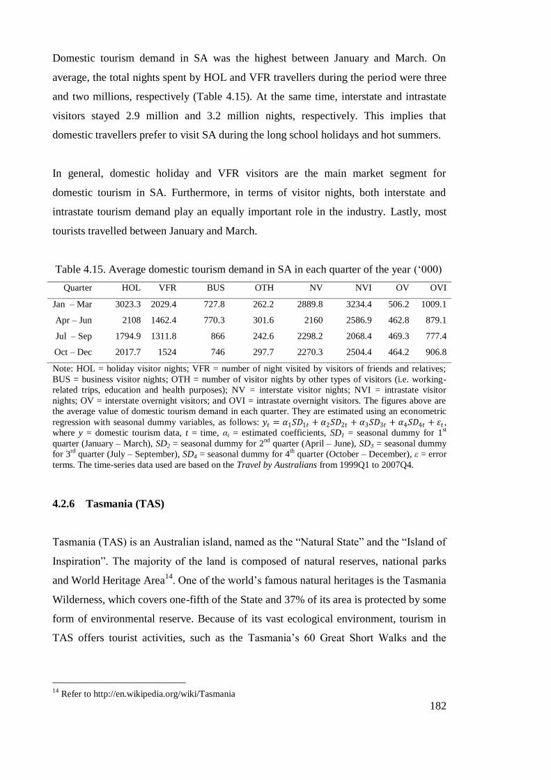
182
Domestic tourism demand in SA was the highest between January and March. On
average, the total nights spent by HOL and VFR travellers during the period were three
and two millions, respectively (Table 4.15). At the same time, interstate and intrastate
visitors stayed 2.9 million and 3.2 million nights, respectively. This implies that
domestic travellers prefer to visit SA during the long school holidays and hot summers.
In general, domestic holiday and VFR visitors are the main market segment for
domestic tourism in SA. Furthermore, in terms of visitor nights, both interstate and
intrastate tourism demand play an equally important role in the industry. Lastly, most
tourists travelled between January and March.
Table 4.15. Average domestic tourism demand in SA in each quarter of the year („000)
Quarter HOL VFR BUS OTH NV NVI OV OVI
Jan – Mar 3023.3 2029.4 727.8 262.2 2889.8 3234.4 506.2 1009.1
Apr – Jun 2108 1462.4 770.3 301.6 2160 2586.9 462.8 879.1
Jul – Sep 1794.9 1311.8 866 242.6 2298.2 2068.4 469.3 777.4
Oct – Dec 2017.7 1524 746 297.7 2270.3 2504.4 464.2 906.8
Note: HOL = holiday visitor nights; VFR = number of night visited by visitors of friends and relatives;
BUS = business visitor nights; OTH = number of visitor nights by other types of visitors (i.e. working-
related trips, education and health purposes); NV = interstate visitor nights; NVI = intrastate visitor
nights; OV = interstate overnight visitors; and OVI = intrastate overnight visitors. The figures above are
the average value of domestic tourism demand in each quarter. They are estimated using an econometric
regression with seasonal dummy variables, as follows: 𝑦𝑡 = 𝛼1𝑆𝐷1𝑡 + 𝛼2𝑆𝐷2𝑡 + 𝛼3𝑆𝐷3𝑡 + 𝛼4𝑆𝐷4𝑡 + 𝜀𝑡 , where y = domestic tourism data, t = time, αi = estimated coefficients, SD1 = seasonal dummy for 1
st
quarter (January – March), SD2 = seasonal dummy for 2nd
quarter (April – June), SD3 = seasonal dummy
for 3rd
quarter (July – September), SD4 = seasonal dummy for 4th quarter (October – December), ε = error
terms. The time-series data used are based on the Travel by Australians from 1999Q1 to 2007Q4.
4.2.6 Tasmania (TAS)
Tasmania (TAS) is an Australian island, named as the “Natural State” and the “Island of
Inspiration”. The majority of the land is composed of natural reserves, national parks
and World Heritage Area14
. One of the world‟s famous natural heritages is the Tasmania
Wilderness, which covers one-fifth of the State and 37% of its area is protected by some
form of environmental reserve. Because of its vast ecological environment, tourism in
TAS offers tourist activities, such as the Tasmania‟s 60 Great Short Walks and the
14
Refer to http://en.wikipedia.org/wiki/Tasmania

183
Great Walks of Tasmania15
, which attract visitors who are nature-seekers, bushwalkers
and nature-adventurers. Furthermore, the state also provides winery tourism where
visitors can experience wine-tasting while enjoying the scenes of national parks16
. It is
the smallest of the Australian States, both in area and population, but it is a relatively
decentralised state.
Holiday visitors (HOL) stayed the most nights in TAS, followed by VFR visitors (Table
4.16). The mean of HOL visitor nights per quarter is 1.2 million, whereas the mean of
VFR visitor nights is about 0.6 million. Between 1999 and 2007, the maximum HOL
and VFR visitor nights in a quarter were 2.7 and 1.8 million, respectively. Even though
the HOL visitor nights are double of VFR visitor nights in TAS, the variation of the
former data is higher than that of the latter data.
BUS and OTH visitors spent fewer nights in TAS compared to HOL and VFR tourists
(Table 4.16). On average, BUS and OTH travellers stayed 307,500 and 93,833 nights in
TAS, respectively, per quarter. During 1999 and 2007, their maximum visitor nights
were between 256,000 and 686,000, respectively. However, in terms of the coefficients
of variation, only the BUS visitor night data are relatively lower than the HOL and VFR
visitor night data.
Table 4.16. Descriptive statistics of domestic tourist markets in TAS („000)
Note: HOL = holiday visitor nights; VFR = number of night visited by visitors of friends and relatives;
BUS = business visitor nights; OTH = number of visitor nights by other types of visitors (i.e. working-
related trips, education and health purposes); NV = interstate visitor nights; NVI = intrastate visitor
nights; OV = interstate overnight visitors; and OVI = intrastate overnight visitors. Max. = maximum; Min
= minimum; S.D. = standard deviation; and C.V. = Coefficient of variation. Source: Quarterly data (1999-
2007) from the quarterly reports of Travel by Australians.
15
Refer to “Australian Geographic: Great walks of Tasmania” and “Tasmania‟s 60 great short walks”
which can be downloaded from http://www.discovertasmania.com/brochures 16
Refer to “Discover Tasmania: Cool wine and food, cool wilderness” which can be downloaded from
http://www.discovertasmania.com/brochures
HOL VFR BUS OTH NV NVI OV OVI
Mean 1209 603.8 307.5 93.8 1485.1 779.3 205.9 300.4
Max. 2693 1750 686 256 3527 1579 343 492
Min. 351 314 179 25 587 441 119 204
S.D. 631.8 282.4 88.6 51.3 693.9 277.3 66.5 67.7
C.V. (%) 52.3 46.8 28.8 54.7 46.7 35.6 32.3 22.5

184
Figure 4.7 highlight trends over time for domestic tourist data in TAS during 1999 and
2007 by purpose of visits. Accordingly, HOL visitor night data displays a very distinct
seasonal pattern with a trend towards greater disparity between high and low seasons.
Similarly, VFR visitor night data shows a pattern of stable seasonality, but there was an
outlier in the first quarter of 2004 where the VFR visitor nights increased from about
400,000 to above 1.6 million. For BUS visitor night data, the overall trend is relatively
constant; however, in 2002, the number of BUS visitor nights surged from below
300,000 to nearly 700,000. In contrast, for the OTH data, there was a sharp increase in
the visitor nights in mid 2002 and early 2006, and, in overall, the data have a fairly
upward trend.
In TAS, interstate tourism is relatively more important than intrastate tourism. In Table
4.16, about 205,917 interstate visitors stayed 1.5 million nights in TAS, while 300,389
Figure 4.7. Numbers of visitor nights by purpose of visits and numbers of interstate and
intrastate visitors in TAS
Panel (A): Holiday visitor nights (HOL)
0
500
1,000
1,500
2,000
2,500
3,000
Mar
-99
No
v-9
9
Jul-
00
Mar
-01
No
v-0
1
Jul-
02
Mar
-03
No
v-0
3
Jul-
04
Mar
-05
No
v-0
5
Jul-
06
Mar
-07
No
v-0
7
'000
HOL
Linear (HOL)
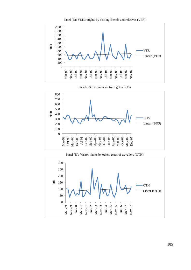
185
Panel (B): Visitor nights by visiting friends and relatives (VFR)
Panel (C): Business visitor nights (BUS)
Panel (D): Visitor nights by others types of travellers (OTH)
0
200
400
600
800
1,000
1,200
1,400
1,600
1,800
2,000
Mar
-99
No
v-9
9
Jul-
00
Mar
-01
No
v-0
1
Jul-
02
Mar
-03
No
v-0
3
Jul-
04
Mar
-05
No
v-0
5
Jul-
06
Mar
-07
No
v-0
7
'000
VFR
Linear (VFR)
0
100
200
300
400
500
600
700
800
Mar
-99
Oct
-99
May
-00
Dec
-00
Jul-
01
Feb
-02
Sep
-02
Apr-
03
No
v-0
3
Jun-0
4
Jan-0
5
Aug-0
5
Mar
-06
Oct
-06
May
-07
Dec
-07
'000
BUS
Linear (BUS)
0
50
100
150
200
250
300
Mar
-99
No
v-9
9
Jul-
00
Mar
-01
No
v-0
1
Jul-
02
Mar
-03
No
v-0
3
Jul-
04
Mar
-05
No
v-0
5
Jul-
06
Mar
-07
No
v-0
7
'000
OTH
Linear (OTH)

186
Panel (E): Interstate visitor nights in TAS
Panel (F): Intrastate visitor nights in TAS
Panel (G): Interstate visitors in TAS
0
500
1000
1500
2000
2500
3000
3500
4000
Mar
-99
No
v-9
9
Jul-
00
Mar
-01
No
v-0
1
Jul-
02
Mar
-03
No
v-0
3
Jul-
04
Mar
-05
No
v-0
5
Jul-
06
Mar
-07
No
v-0
7
'000
Interstate
Linear (Interstate)
0
200
400
600
800
1000
1200
1400
1600
1800
Mar
-99
No
v-9
9
Jul-
00
Mar
-01
No
v-0
1
Jul-
02
Mar
-03
No
v-0
3
Jul-
04
Mar
-05
No
v-0
5
Jul-
06
Mar
-07
No
v-0
7
'000
Intrastate
Linear (Intrastate)
0
50
100
150
200
250
300
350
400
Mar
-99
No
v-9
9
Jul-
00
Mar
-01
No
v-0
1
Jul-
02
Mar
-03
No
v-0
3
Jul-
04
Mar
-05
No
v-0
5
Jul-
06
Mar
-07
No
v-0
7
'000
Interstate
Linear (Interstate)

187
Panel (H): Intrastate visitors in TAS
Note: The figures above are computed using quarterly time-series data which are extracted from Travel by
Australians, published by Tourism Research Australia (TRA). The linear line in each panel is generated
using a trend regression, which is written as follows: 𝑦𝑡 = 𝛼1 + 𝛼2𝑡 + 𝜀𝑡 , where y = domestic tourism
data, t = time trend, α1,2 = estimated coefficients, ε = error term. The main intention of estimating the
linear trend is to observe the long-term trend of the data.
intrastate visitors spent 779,250 nights. On average, each interstate visitor stayed about
seven nights in the state, whereas it was 2.5 nights for each intrastate visitor. Moreover,
the maximum amount of nights stayed by interstate visitors in TAS was 3.5 million,
which is approximately double the maximum nights stayed by intrastate visitors.
Nonetheless, the coefficient of variation figures in Table 4.16 reveal that the interstate
visitor night data is more volatile than the intrastate visitor night data.
Furthermore, Figure 4.7 demonstrates that strong seasonal patterns exist in both
interstate and intrastate tourism data. However, both datasets display a trend that is
distinct from each other. The interstate tourist arrivals and visitor night data show an
upward growth, whereas the intrastate visitor and visitor night data present a less
extreme downward trend. Therefore, this indicates that tourism in TAS has experienced
an increasing demand from interstate but a dwindling number of intrastate trips.
Another interesting finding is that domestic visitors travelled in TAS during January to
March (the summer season in Australia). In Table 4.17, the number of HOL visitor
nights was recorded about 2.1 million during the period. In addition, VFR and OTH
visitors spent approximately 927,111 and 124,333 nights, respectively, in the peak
season. Similarly, the numbers of interstate and intrastate visitor nights during January
0
100
200
300
400
500
600
Mar
-99
No
v-9
9
Jul-
00
Mar
-01
No
v-0
1
Jul-
02
Mar
-03
No
v-0
3
Jul-
04
Mar
-05
No
v-0
5
Jul-
06
Mar
-07
No
v-0
7
'000
Intrastate
Linear (Intrastate)

188
and March were about 1.7 to 1.8 times the numbers during October to December.
Hence, because of the cooler weather during summer, this makes TAS as an ideal
destination for domestic holidays.
Table 4.17. Average domestic tourism demand in TAS in each quarter of the year („000)
Quarter HOL VFR BUS OTH NV NVI OV OVI
Jan – Mar 2143.3 927.1 296 124.3 2355.6 1197.9 271.2 395.7
Apr – Jun 1084.3 550.9 279.8 85.2 1354 717.3 200.2 291.6
Jul – Sep 578.1 396.7 344.9 76.7 872 561.9 147.7 243.8
Oct – Dec 1030.1 540.3 309.3 89.1 1358.7 639.9 204.6 270.6
Note: HOL = holiday visitor nights; VFR = number of night visited by visitors of friends and relatives;
BUS = business visitor nights; OTH = number of visitor nights by other types of visitors (i.e. working-
related trips, education and health purposes); NV = interstate visitor nights; NVI = intrastate visitor
nights; OV = interstate overnight visitors; and OVI = intrastate overnight visitors. The figures above are
the average value of domestic tourism demand in each quarter. They are estimated using an econometric
regression with seasonal dummy variables, as follows: 𝑦𝑡 = 𝛼1𝑆𝐷1𝑡 + 𝛼2𝑆𝐷2𝑡 + 𝛼3𝑆𝐷3𝑡 + 𝛼4𝑆𝐷4𝑡 + 𝜀𝑡 , where y = domestic tourism data, t = time, αi = estimated coefficients, SD1 = seasonal dummy for 1
st
quarter (January – March), SD2 = seasonal dummy for 2nd
quarter (April – June), SD3 = seasonal dummy
for 3rd
quarter (July – September), SD4 = seasonal dummy for 4th quarter (October – December), ε = error
terms. The time-series data used are based on the Travel by Australians from 1999Q1 to 2007Q4.
4.2.7 Victoria (VIC)
Victoria (VIC) is a densely urbanized and highly centralised state, with an estimated
population of 5.2 million17
. Despite its small land size compared to other Australia
States, the tourist destinations in VIC are well-known for city shopping, winery,
heritage tourism, scenic driving, water-sport activities, and golf tourism. For instance,
Melbourne, the capital city of VIC, is famous for its shopping tourism and iconic
buildings such as the Crown Casino and Eureka Tower. The popular regions are the
Dandenong Rangers, Gippsland, the Grampian region, the Great Ocean Road,
Mornington Peninsula, the Murray, Philips Island and the Yarra Valley, where tourists
can visit wineries, natural attractions (i.e. The Twelve Apostles and the Fairy Penguins),
historical towns and beaches18
.
The main domestic tourist markets in VIC are visitors who are holidaying (HOL),
visiting friends and relatives (VFR), and travelling for business (BUS). Between 1999
and 2007, HOL visitors stayed an average of 6.4 million nights per quarter, whereas
17
Refer to http://en.wikipedia.org/wiki/Victoria_(Australia) 18
More information can be downloaded from http://www.visitvictoria.com.

189
VFR and BUS visitors stayed 4.5 and 1.8 million nights, respectively (Table 4.18). The
highest number of nights recorded in the period was 11.2 million nights by HOL
travellers, showing that HOL visitors are the most important market segment for
domestic tourism in VIC. Nevertheless, among others, the HOL visitor night data
presents the highest percentage of coefficient of variation.
Table 4.18. Descriptive statistics of domestic tourist markets in VIC („000)
Note: HOL = holiday visitor nights; VFR = number of night visited by visitors of friends and relatives;
BUS = business visitor nights; OTH = number of visitor nights by other types of visitors (i.e. working-
related trips, education and health purposes); NV = interstate visitor nights; NVI = intrastate visitor
nights; OV = interstate overnight visitors; and OVI = intrastate overnight visitors. Max. = maximum; Min
= minimum; S.D. = standard deviation; and C.V. = Coefficient of variation. Source: Quarterly data (1999-
2007) from the quarterly reports of Travel by Australians.
Seasonality is evident in the HOL and VFR visitor night data [Figure 4.8 (Panels A and
B)]. The peak season for these two groups of visitors is between January and March.
The same is true for BUS and OTH visitor night data [Figure 4.8 (Panels C and D)];
however, they are unpredictable. For instance, there were two drastic decreases in the
number of BUS visitor nights in the first quarters of 2005 and 2006. Moreover, the OTH
data fluctuate strongly between 2001 and 2003 but they remain stable thereafter.
For interstate and intrastate tourism demand in VIC, Table 4.18 shows that intrastate
tourists spent more nights travelling in VIC than interstate tourists. Accordingly,
average intrastate visitor nights per quarter from 1999 to 2007 were 8.1 million, while it
was 5.4 million nights for interstate tourists. However, the average nights spent per
intrastate visitor (2.6) is lower than the average nights spent per interstate visitor (4.3).
There are significant seasonal fluctuations in both interstate and intrastate tourism in
VIC [Figure 4.8 (Panels E - H)]. Nevertheless, the total number of nights spent by
interstate visitors has been relatively constant, despite that the number of interstate
overnight travellers to VIC has increased gradually since 1999. As for intrastate visitors,
HOL VFR BUS OTH NV NVI OV OVI
Mean 6415.9 4594.4 1807 579.6 5410.9 8106.1 1255.6 3137
Max. 11186 6364 2226 1056 6806 12772 1466 4023
Min. 4057 3388 1258 349 4110 5774 1040 2431
S.D. 2265.3 934 258 171.6 879.6 2280.6 119.1 456.7
C.V. (%) 35.3 20.3 14.3 29.6 16.3 28.1 9.5 14.6

190
the number of visitor nights has been at a declining rate. Similarly, there has been a
slow and long-term decrease in the number of intrastate overnight visitors.
Figure 4.8. Numbers of visitor nights by purpose of visits and numbers of interstate and
intrastate visitors in VIC
Panel (A): Holiday visitor nights (HOL)
Panel (B): Visitor nights by visiting friends and relatives (VFR)
Panel (C): Business visitor nights (BUS)
0
2,000
4,000
6,000
8,000
10,000
12,000
Mar
-99
No
v-9
9
Jul-
00
Mar
-01
No
v-0
1
Jul-
02
Mar
-03
No
v-0
3
Jul-
04
Mar
-05
No
v-0
5
Jul-
06
Mar
-07
No
v-0
7
'000
HOL
Linear (HOL)
0
1,000
2,000
3,000
4,000
5,000
6,000
7,000
Mar
-99
No
v-9
9
Jul-
00
Mar
-01
No
v-0
1
Jul-
02
Mar
-03
No
v-0
3
Jul-
04
Mar
-05
No
v-0
5
Jul-
06
Mar
-07
No
v-0
7
'000
VFR
Linear (VFR)
0
500
1,000
1,500
2,000
2,500
Mar
-99
No
v-9
9
Jul-
00
Mar
-01
No
v-0
1
Jul-
02
Mar
-03
No
v-0
3
Jul-
04
Mar
-05
No
v-0
5
Jul-
06
Mar
-07
No
v-0
7
'000
BUS
Linear (BUS)

191
Panel (D): Visitor nights by other types of travellers (OTH)
Panel (E): Interstate visitor nights in VIC
Panel (F): Intrastate visitor nights in VIC
0
200
400
600
800
1,000
1,200
Mar
-99
No
v-9
9
Jul-
00
Mar
-01
No
v-0
1
Jul-
02
Mar
-03
No
v-0
3
Jul-
04
Mar
-05
No
v-0
5
Jul-
06
Mar
-07
No
v-0
7
'000
OTH
Linear (OTH)
0
1000
2000
3000
4000
5000
6000
7000
8000
Mar
-99
No
v-9
9
Jul-
00
Mar
-01
No
v-0
1
Jul-
02
Mar
-03
No
v-0
3
Jul-
04
Mar
-05
No
v-0
5
Jul-
06
Mar
-07
No
v-0
7
'000
Interstate
Linear (Interstate)
0
2000
4000
6000
8000
10000
12000
14000
Mar
-99
No
v-9
9
Jul-
00
Mar
-01
No
v-0
1
Jul-
02
Mar
-03
No
v-0
3
Jul-
04
Mar
-05
No
v-0
5
Jul-
06
Mar
-07
No
v-0
7
'000
Intrastate
Linear (Intrastate)
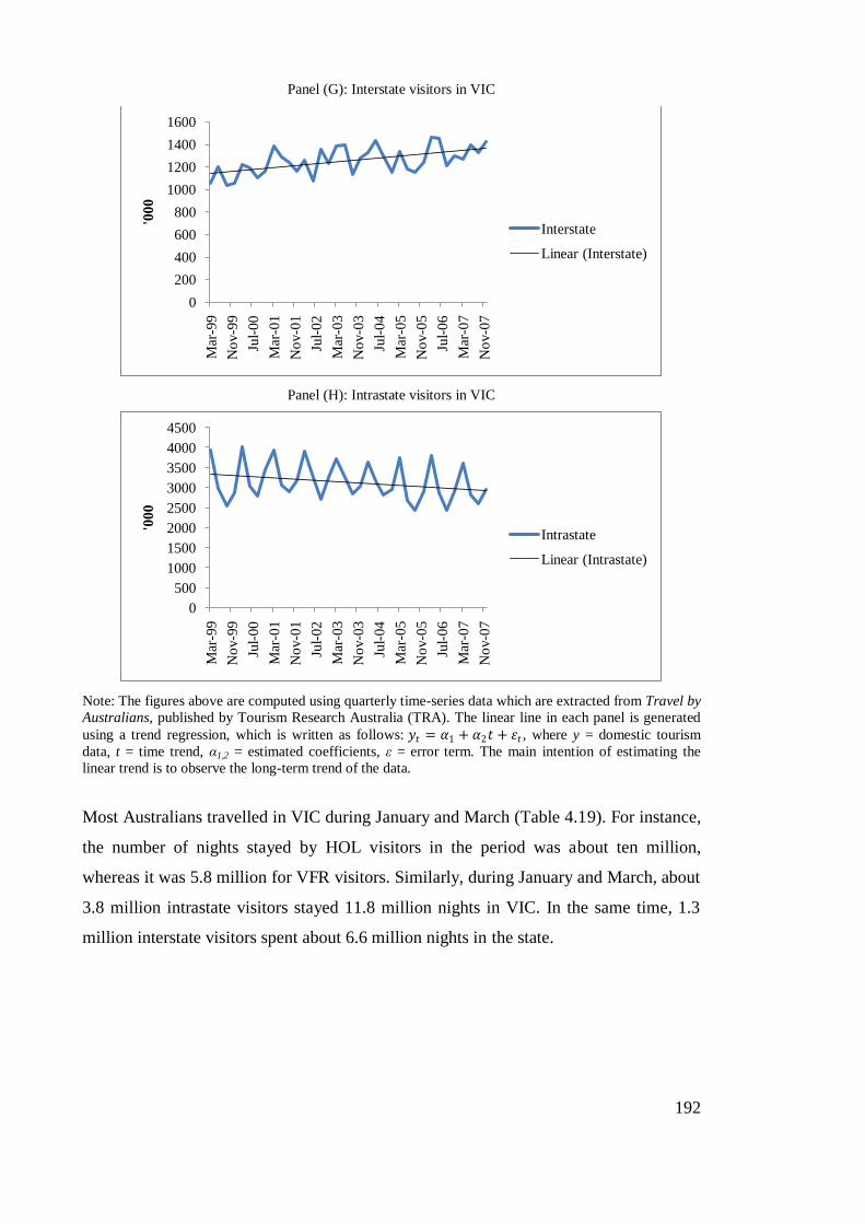
192
Panel (G): Interstate visitors in VIC
Panel (H): Intrastate visitors in VIC
Note: The figures above are computed using quarterly time-series data which are extracted from Travel by
Australians, published by Tourism Research Australia (TRA). The linear line in each panel is generated
using a trend regression, which is written as follows: 𝑦𝑡 = 𝛼1 + 𝛼2𝑡 + 𝜀𝑡 , where y = domestic tourism
data, t = time trend, α1,2 = estimated coefficients, ε = error term. The main intention of estimating the
linear trend is to observe the long-term trend of the data.
Most Australians travelled in VIC during January and March (Table 4.19). For instance,
the number of nights stayed by HOL visitors in the period was about ten million,
whereas it was 5.8 million for VFR visitors. Similarly, during January and March, about
3.8 million intrastate visitors stayed 11.8 million nights in VIC. In the same time, 1.3
million interstate visitors spent about 6.6 million nights in the state.
0
200
400
600
800
1000
1200
1400
1600
Mar
-99
No
v-9
9
Jul-
00
Mar
-01
No
v-0
1
Jul-
02
Mar
-03
No
v-0
3
Jul-
04
Mar
-05
No
v-0
5
Jul-
06
Mar
-07
No
v-0
7
'000
Interstate
Linear (Interstate)
0
500
1000
1500
2000
2500
3000
3500
4000
4500
Mar
-99
No
v-9
9
Jul-
00
Mar
-01
No
v-0
1
Jul-
02
Mar
-03
No
v-0
3
Jul-
04
Mar
-05
No
v-0
5
Jul-
06
Mar
-07
No
v-0
7
'000
Intrastate
Linear (Intrastate)
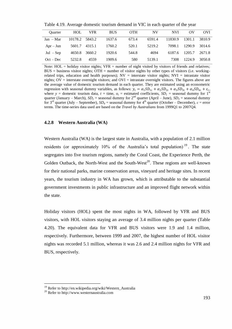
193
Table 4.19. Average domestic tourism demand in VIC in each quarter of the year
Quarter HOL VFR BUS OTH NV NVI OV OVI
Jan – Mar 10178.2 5843.2 1637.6 673.4 6591.4 11830.9 1301.1 3810.9
Apr – Jun 5601.7 4315.1 1760.2 520.1 5219.2 7098.1 1290.9 3014.6
Jul – Sep 4650.8 3660.2 1920.6 544.8 4694 6187.6 1205.7 2671.8
Oct – Dec 5232.8 4559 1909.6 580 5139.1 7308 1224.9 3050.8
Note: HOL = holiday visitor nights; VFR = number of night visited by visitors of friends and relatives;
BUS = business visitor nights; OTH = number of visitor nights by other types of visitors (i.e. working-
related trips, education and health purposes); NV = interstate visitor nights; NVI = intrastate visitor
nights; OV = interstate overnight visitors; and OVI = intrastate overnight visitors. The figures above are
the average value of domestic tourism demand in each quarter. They are estimated using an econometric
regression with seasonal dummy variables, as follows: 𝑦𝑡 = 𝛼1𝑆𝐷1𝑡 + 𝛼2𝑆𝐷2𝑡 + 𝛼3𝑆𝐷3𝑡 + 𝛼4𝑆𝐷4𝑡 + 𝜀𝑡 , where y = domestic tourism data, t = time, αi = estimated coefficients, SD1 = seasonal dummy for 1
st
quarter (January – March), SD2 = seasonal dummy for 2nd
quarter (April – June), SD3 = seasonal dummy
for 3rd
quarter (July – September), SD4 = seasonal dummy for 4th quarter (October – December), ε = error
terms. The time-series data used are based on the Travel by Australians from 1999Q1 to 2007Q4.
4.2.8 Western Australia (WA)
Western Australia (WA) is the largest state in Australia, with a population of 2.1 million
residents (or approximately 10% of the Australia‟s total population)19
. The state
segregates into five tourism regions, namely the Coral Coast, the Experience Perth, the
Golden Outback, the North-West and the South-West20
. These regions are well-known
for their national parks, marine conservation areas, vineyard and heritage sites. In recent
years, the tourism industry in WA has grown, which is attributable to the substantial
government investments in public infrastructure and an improved flight network within
the state.
Holiday visitors (HOL) spent the most nights in WA, followed by VFR and BUS
visitors, with HOL visitors staying an average of 3.4 million nights per quarter (Table
4.20). The equivalent data for VFR and BUS visitors were 1.9 and 1.4 million,
respectively. Furthermore, between 1999 and 2007, the highest number of HOL visitor
nights was recorded 5.1 million, whereas it was 2.6 and 2.4 million nights for VFR and
BUS, respectively.
19
Refer to http://en.wikipedia.org/wiki/Western_Australia 20
Refer to http://www.westernaustralia.com

194
Table 4.20. Descriptive statistics of domestic tourist markets in WA („000)
Note: HOL = holiday visitor nights; VFR = number of night visited by visitors of friends and relatives;
BUS = business visitor nights; OTH = number of visitor nights by other types of visitors (i.e. working-
related trips, education and health purposes); NV = interstate visitor nights; NVI = intrastate visitor
nights; OV = interstate overnight visitors; and OVI = intrastate overnight visitors. Max. = maximum; Min
= minimum; S.D. = standard deviation; and C.V. = Coefficient of variation. Source: Quarterly data (1999-
2007) from the quarterly reports of Travel by Australians.
In Figure 4.9, the HOL visitor night data shows a constant trend. Conversely, BUS
visitor night data reveals a gradual growth, which could relate to the WA mining boom
which attracted more business travellers to WA. Similarly, VFR and OTH visitor night
data displays an increasing trend between 1999 and 2007. Hence, the figures above
conclude that domestic overnight tourism in WA performed well in the past nine years.
Intrastate tourism demand in WA is higher than interstate tourism demand (Table 4.20).
Accordingly, intrastate visitors stayed 5 million nights per quarter of a year in WA,
whereas interstate visitors spent 2.4 million nights. In addition, 1.4 million intrastate
overnight visitors travelled within WA, while 253,278 interstate overnight visitors
travelled to WA. However, in terms of average nights stayed per visitor, each intrastate
visitor spent fewer nights (3.4 nights) than an interstate visitor (9.5 nights).
Referring to Figure 4.9, the demand for interstate tourism in WA is growing while, for
intrastate tourism, it is somewhat stable. For instance, the number of interstate visitor
nights in WA shows an upward trend since 2004 while there was a steady trend in
intrastate visitor nights in 2002. Nonetheless, while the number of interstate overnight
visitors has increased dramatically, the number of intrastate overnight visitors in WA
shows a slight declining trend, particularly since 2001.
HOL VFR BUS OTH NV NVI OV OVI
Mean 3403.7 1943.6 1428 342.4 2395.9 5039.4 253.3 1367.6
Max. 5131 2567 2364 514 3721 6312 347 1613
Min. 2478 1357 622 170 1375 4303 141 1156
S.D. 598.3 284 374.4 86.7 585.1 427.7 51.7 112.5
C.V. (%) 17.6 14.6 26.2 25.3 24.4 8.5 20.4 8.2
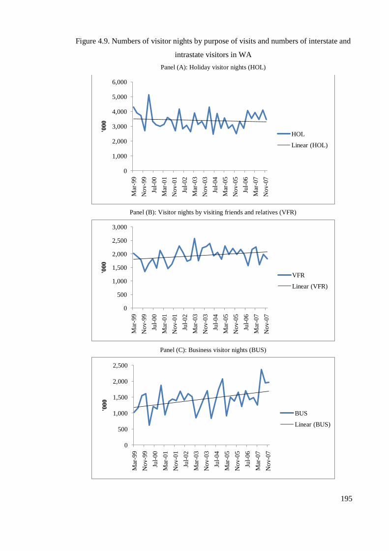
195
Figure 4.9. Numbers of visitor nights by purpose of visits and numbers of interstate and
intrastate visitors in WA
Panel (A): Holiday visitor nights (HOL)
Panel (B): Visitor nights by visiting friends and relatives (VFR)
Panel (C): Business visitor nights (BUS)
0
1,000
2,000
3,000
4,000
5,000
6,000
Mar
-99
No
v-9
9
Jul-
00
Mar
-01
No
v-0
1
Jul-
02
Mar
-03
No
v-0
3
Jul-
04
Mar
-05
No
v-0
5
Jul-
06
Mar
-07
No
v-0
7
'000
HOL
Linear (HOL)
0
500
1,000
1,500
2,000
2,500
3,000
Mar
-99
No
v-9
9
Jul-
00
Mar
-01
No
v-0
1
Jul-
02
Mar
-03
No
v-0
3
Jul-
04
Mar
-05
No
v-0
5
Jul-
06
Mar
-07
No
v-0
7
'000
VFR
Linear (VFR)
0
500
1,000
1,500
2,000
2,500
Mar
-99
No
v-9
9
Jul-
00
Mar
-01
No
v-0
1
Jul-
02
Mar
-03
No
v-0
3
Jul-
04
Mar
-05
No
v-0
5
Jul-
06
Mar
-07
No
v-0
7
'000
BUS
Linear (BUS)

196
Panel (D): Visitor nights by other types of travellers (OTH)
Panel (E): Interstate visitor nights in WA
Panel (F): Intrastate visitor nights in WA
0
100
200
300
400
500
600
Mar
-99
Oct
-99
May
-00
Dec
-00
Jul-
01
Feb
-02
Sep
-02
Apr-
03
No
v-0
3
Jun-0
4
Jan-0
5
Aug-0
5
Mar
-06
Oct
-06
May
-07
Dec
-07
'000
OTH
Linear (OTH)
0
500
1000
1500
2000
2500
3000
3500
4000
Mar
-99
No
v-9
9
Jul-
00
Mar
-01
No
v-0
1
Jul-
02
Mar
-03
No
v-0
3
Jul-
04
Mar
-05
No
v-0
5
Jul-
06
Mar
-07
No
v-0
7
'000
Interstate
Linear (Interstate)
0
1000
2000
3000
4000
5000
6000
7000
Mar
-99
No
v-9
9
Jul-
00
Mar
-01
No
v-0
1
Jul-
02
Mar
-03
No
v-0
3
Jul-
04
Mar
-05
No
v-0
5
Jul-
06
Mar
-07
No
v-0
7
'000
Intrastate
Linear (Intrastate)

197
Panel (G): Interstate visitor nights in WA
Panel (H): Intrastate visitor nights in WA
Note: The figures above are computed using quarterly time-series data which are extracted from Travel by
Australians, published by Tourism Research Australia (TRA). The linear line in each panel is generated
using a trend regression, which is written as follows: 𝑦𝑡 = 𝛼1 + 𝛼2𝑡 + 𝜀𝑡 , where y = domestic tourism
data, t = time trend, α1,2 = estimated coefficients, ε = error term. The main intention of estimating the
linear trend is to observe the long-term trend of the data.
In addition, unlike some other States and Territories, the travel season to WA varies
from one type of visitors to another. Accordingly, the peak months for HOL, VFR and
intrastate visitors travelling in WA are from January to March (Table 4.21). This could
be associated with the summer school holidays in Australia. Meanwhile, BUS and
interstate visitor nights peaked during spring (from October to December), prior to the
hottest months.
0
50
100
150
200
250
300
350
400
Mar
-99
No
v-9
9
Jul-
00
Mar
-01
No
v-0
1
Jul-
02
Mar
-03
No
v-0
3
Jul-
04
Mar
-05
No
v-0
5
Jul-
06
Mar
-07
No
v-0
7
'000
Interstate
Linear (Interstate)
0
200
400
600
800
1000
1200
1400
1600
1800
Mar
-99
No
v-9
9
Jul-
00
Mar
-01
No
v-0
1
Jul-
02
Mar
-03
No
v-0
3
Jul-
04
Mar
-05
No
v-0
5
Jul-
06
Mar
-07
No
v-0
7
'000
Intrastate
Linear (Intrastate)

198
Table 4.21. Average domestic tourism demand in WA in each quarter of the year („000)
Quarter HOL VFR BUS OTH NV NVI OV OVI
Jan – Mar 3977.7 2168 1037.2 306.6 2142.8 5444.6 241.8 1419.8
Apr – Jun 3170 1832.9 1463.6 346.3 2026.9 4893.2 244.8 1390.2
Jul – Sep 3540.4 1852.2 1515.9 374.6 2585.6 5135.6 263.4 1312.7
Oct – Dec 2926.6 1921.1 1695.4 342.3 2828.3 4684.3 263.1 1347.8
Note: HOL = holiday visitor nights; VFR = number of night visited by visitors of friends and relatives;
BUS = business visitor nights; OTH = number of visitor nights by other types of visitors (i.e. working-
related trips, education and health purposes); NV = interstate visitor nights; NVI = intrastate visitor
nights; OV = interstate overnight visitors; and OVI = intrastate overnight visitors. The figures above are
the average value of domestic tourism demand in each quarter. They are estimated using an econometric
regression with seasonal dummy variables, as follows: 𝑦𝑡 = 𝛼1𝑆𝐷1𝑡 + 𝛼2𝑆𝐷2𝑡 + 𝛼3𝑆𝐷3𝑡 + 𝛼4𝑆𝐷4𝑡 + 𝜀𝑡 , where y = domestic tourism data, t = time, αi = estimated coefficients, SD1 = seasonal dummy for 1
st
quarter (January – March), SD2 = seasonal dummy for 2nd
quarter (April – June), SD3 = seasonal dummy
for 3rd
quarter (July – September), SD4 = seasonal dummy for 4th quarter (October – December), ε = error
terms. The time-series data used are based on the Travel by Australians from 1999Q1 to 2007Q4.
4.3 Conclusion
Domestic overnight visitors in Australia have higher average expenditure than domestic
day visitors, indicating that the former is one of the important market segments in
Australian tourism. The main objective of this chapter was to examine the market trends
and seasonality of domestic overnight trips in eight Australian States and the major
populated Territories. Six types of domestic overnight tourists have been considered,
which are comprised of interstate tourist arrivals, intrastate visitors, holiday-makers,
business travellers, visitors who are visiting friends and relatives, and other visitors.
Some of the main points, which have been noted in Section 4.2, are listed in Table 4.22.
Overall, the analysis has provided insightful information about the demand for domestic
overnight tourism demand in each of these Australian States and Territories. First,
domestic holiday tourist is the most important market segment for all States, except
Australian Capital Territory. Particularly in Tasmania, there was a growth in the number
of holiday visitor nights in the state. Second, most domestic tourists travelled to the
northern states of Australia during winter, whereas they travelled to the southern states
of Australia mostly during summer. However, there is no distinct travel season for
domestic visitors in WA. Lastly, there is evidence that the demand for domestic
overnight tourism in some states has declined, especially in New South Wales and
South Australia.

199
Table 4.22. A summary of domestic overnight tourism demand in each Australia States
State Main market
segment(s) Main points
ACT VFR - When an unexpected event occurred, the
numbers of HOL and VFR visitors increased
noticeably. - The major period for all visitor groups
visiting ACT was January to March.
NSW HOL, VFR and
Intrastate visitors - BUS and VFR visitor night data show a
declining trend. - Intrastate visitors spent more nights than
interstate visitors; however, the demand for
intrastate tourism has declined since 2005. - The peak season for most travellers within
NSW was between January and March; the
exceptions were BUS and OTH visitors.
NT HOL, BUS and
Interstate tourists - Domestic visitor numbers were high in all
seasons except during summer (from January
to March).
QLD HOL, VFR and BUS - The peak period for travellers in QLD was
winter (from July to September) because of
the mild and sunny weather. - There was a continuous growth in interstate
tourist arrivals to QLD from 1999 to 2007
and strong seasonality.
SA HOL and VFR - Declining trends for BUS, VFR and intrastate
tourism demand. - Most visitors travelled in SA between January
and March.
TAS HOL and Interstate
tourists - HOL visitor night and interstate visitor data
display an increasing trend. - The peak season for domestic visitors
travelling in TAS was during January to
March.
VIC HOL, VFR, BUS and
Intrastate tourists - Significant seasonality exists for HOL and
VFR visitor night data. - The average night spent per interstate visitor
was higher than the average night spent per
intrastate visitor. - The number of interstate visitors has
increased gradually since 1999. However,
there was a slight declining trend for
intrastate trips in VIC. - Most Australians travelled in VIC during
January to March.

200
State Main market
segment(s) Main points
WA HOL and Intrastate
tourists - BUS visitor night data display a gradual
increase while the VFR visitor night data
show a downward trend. - The total interstate trips to WA are lower than
the total intrastate trips in WA. However, on
average, an interstate visitor spent more
nights than an intrastate visitor.
Note: ACT – Australian Capital Territory, NSW- New South Wales, NT – Northern Territory,
QLD – Queensland, SA – South Australia, TAS – Tasmania, VIC – Victoria, WA – Western
Australia, BUS - business tourism, HOL - holiday tourism, and VFR – visitors who are visiting
friends and relatives. The full details of Australian tourism demand analysis can be found in the
body text of Chapter 4.
201
Chapter 5
Modelling Australian domestic tourism
demand (I): A preliminary study
5.1 Motivation
In the early study of Australian domestic tourism demand, the pioneer paper in the
literature is Hamal (1996). Using the Johansen cointegration analysis, the research
estimated the demand determinants of domestic tourism in Australia.
One of the main problems that emerged in Hamal‟s study is that only 18 observations
were used. Such a small data sample used in this time-series analysis could yield
inaccurate estimation. This is because, according to Lim (2006), a reasonably large
sample size is the time-series statistical requirement for the estimates to be asymptotic.
It is surprising that, even though the sample data used in the study was small, the
estimates revealed correct signs that supported the prior expectations of consumer
demand theory. Nevertheless, Hamal (1996) suspected that the results might not be
reliable and suggested that his study requires re-examination, by increasing the sample
size.
This chapter attempts to re-examine domestic tourism demand using Hamal‟s
suggestion. The main motivation is to evaluate whether increasing the sample size could
still generate demand coefficients with the correct signs and with support from the
diagnostic tests.
5.2 Modelling Interstate Domestic Tourism Demand in Australia
Interstate tourism is an important component of the domestic tourism business in
Australia. However, empirical analyses of interstate tourism demand have not been
previously undertaken. The motivation for this research is to investigate the short- and
long-run causal relationships between economic factors and interstate tourism demand

202
in Australia. Using a cointegration approach, this study discovers two distinct results.
First, Australian household income, accommodation prices, the prices of recreation and
restaurants, and domestic airfares have significant impacts on the demand in the short-
run. Second, some of the long-run economic coefficients show incorrect signs, which
contradicts the theory of consumer demand.
According to the literature on tourism demand considered in Chapter Two, an interstate
tourism demand model can be written as follows:
),,,,,( OCDAFRRACCYfDIT
where DIT = interstate tourism demand, Y = income, ACC = price of tourist
accommodation, RR = prices of recreation and restaurants, F = price of fuel, DA =
domestic airfares and OC = prices of overseas holidays.
Data on interstate tourism demand can be obtained from Travel by Australians, which is
produced quarterly by Tourism Research Australia. In this research, data on interstate
visitor nights will be employed. For economic variables, gross domestic product (GDP)
per capita is employed as a proxy for income variable. For prices of tourism goods and
services in Australia, data on average price of accommodation per night and household
expenditure on recreation, restaurant and cafes are used. In addition, the consumer price
index (CPI) of automotive fuel and domestic economy airfares are used as a proxy
variable for domestic transportation costs. This paper also employs data on the CPI of
overseas holidays, travel and accommodation to represent the price of substitutes for
interstate travel. All the above economic data are available on a quarterly basis from
quarter 3 of 1998 to quarter 4 of 2006 and can be obtained from the websites of the
Australian Bureau of Statistics (ABS) and Department of Transport and Regional
Services (DOTARS).
The interstate tourism demand model is specified as a log-linear model because it is
easy to interpret the estimated coefficients in terms of elasticities [Lim (1997)]. In fact,
log-linear models have been widely used in the literature on tourism demand [Lim and
McAleer (2001) and Seddighi and Shearing (1997)].

203
5.2.1 Unit root tests
In this chapter, an augmented Dickey-Fuller (ADF) test is used, which is written as
follows:
1
1
1
p
i
tititt etzzz
where z = time series of a variable, t = time trend, p = number of lag value and e = error
term. The hypotheses of the ADF test are specified as follows:
Ho: = 0 H1: 0
If the null hypothesis is not rejected, this implies that the data is non-stationary.
Conversely, the rejection of the null hypothesis indicates that the data is stationary or
I(0). Song and Witt (2000) highlighted that it is important to select the appropriate lag
length for all time series data because the ADF test tends to over-reject the null
hypothesis when using too few lags or to reduce degrees of freedom when there are too
many lags. This paper employs the Akaike information criterion (AIC) and Schwarz
Bayesian criterion (SBC) as the criteria for selecting the lag length of the ADF test.
Nevertheless, Phillips and Perron (1990) argued that ADF test is rather restrictive
because the test assumes no autocorrelation and heteroscedesticity in the estimated
residuals. Hence, the Phillips-Perron (PP) test will be employed because the test relaxes
the above-mentioned assumptions.
The ADF test statistics in Table 5.1 and 5.2 show that the logarithms and log-difference
of DIT, Y and RR are I(0), but I (1) for ACC, F, DA and OC. Based on the ADF test
results, the conclusion is that the first difference of all variables do not have the same
order of integration. However, the PP test statistics in Table 5.1 and 5.2 reveal a
different perspective. The logarithms of ACC, F, DA and OC are I(1) and the rest of the
variables are I(0). Eventually, all variables become I(0) after taking the first difference.
In other words, the results of PP test imply that the first difference of all variables have
the same order of integration.

204
Table 5.1. Unit root test statistics for economic variables in logarithms
Variable
ADF test
Lag length of ADF PP test
DIT
-3.518
1
-10.408
Y -3.636 0 -3.723
ACC -2.179* 4 -2.803*
RR -5.831 0 -9.107
F -2.825* 4 -2.321*
DA -2.412* 4 -2.236*
OC
-1.381*
3
-1.729*
Note: Critical values at 5% for ADF and PP tests are -3.573 and -3.551, respectively.
* denotes null hypothesis is not rejected at 5% significant level.
Table 5.2. Unit root test statistics for economic variables in log-differences
Variable
ADF test
Lag length of ADF
PP test
DIT
-5.190
1
-33.289
Y -5.487 0 -6.093
ACC -2.795* 4 -7.307
RR -6.914 0 -14.602
F -2.448* 4 -4.850
DA -2.564* 4 -4.840
OC -1.800* 4 -5.441
Notes: Critical values at 5% for ADF and PP tests are -3.580 and -3.556, respectively. * denotes null
hypothesis is not rejected at 5% significant level.
In the literature of international tourism demand, Chan et al. (2005) and Shareef and
McAleer (2007) preferred the PP test over the ADF test. They asserted that PP test has
higher power in finite samples than ADF test. Hence, this study prefers the results of PP
test which concludes that the same order of integration exists in all economic variables.
Given the above results, cointegration analysis can be carried out.
5.2.2 Cointegration analysis
A time-series 𝑦𝑡 is said to be I(1) if Δ𝑦𝑡 is stationary time-series [I(0)]. Suppose that
𝑦𝑡 = 𝛽1𝑥𝑡 + 𝑢𝑡 where 𝑦𝑡~𝐼(1) , 𝑥𝑡~𝐼(1) , 𝑢𝑡~𝐼(0) , then 𝑦𝑡 = 𝛽1𝑥𝑡 + 𝑢𝑡 ~ 𝐼(1) .
Nevertheless, 𝑦𝑡 and 𝑥𝑡 are said to be cointegrated if there exists 𝛽1 such that
𝑦𝑡 − 𝛽1𝑥𝑡 = 𝑢𝑡 ~ 𝐼(0). This means that 𝑦𝑡 and 𝑥𝑡 do not drift too far apart from each

205
other over time, and there is a long-run equilibrium relationship between them [See
Maddala (2003) for more information].
The regression of interstate tourism demand can be expressed as follows:
OCDAFRRACCYDIT 7654321
Hence, according to consumer demand theory, the signs of the parameters are expected
to be 2 >0, 3 < 0, 4 < 0, 5 <0, 6 < 0 and 7 > 0. Cointegration analysis is to
examine whether these variables will be cointegrated. To do that, this research considers
Johansen‟s (1995) cointegration and error-correction methods. The purpose of these
methods is to generate long-run relationships among the economic variables.
Furthermore, they can provide long-run and short-run estimations for the purpose of
long-term tourism planning and short-term business forecasting [Song and Witt (2000)].
Another benefit of using Johansen‟s cointegration is that it can be applied to a set of
variables containing possibly a mixture of I(0) and I(1) regressors21
[Johansen (1995)
and Motamed et al. (2008)]. These methods have been widely used in the context of
international tourism demand to Australia [Kulendran and King (1997) and Lim and
McAleer (2001)], but have not been applied in the demand analysis of intrastate and
interstate tourism.
The basic model used in the Johansen cointegration analysis is a vector autoregressive
(VAR) model, which is developed by Sims (1980). Unlike single equation models, this
model treats all variables as endogenous [Song and Witt (2006)]. The model has been
employed for international tourism demand, for example, by De Mello and Nell (2005)
and Song and Witt (2006).
21
Hjalmarsson and Österholm (2007) argued that the presence of stationary or near unit-root process
variables in Johansen‟s cointegration has a substantial probability of falsely concluding the existence of
cointegration relations among the I(1) and I(0) variables. However, when Motamed et al. (2008)
employed I(1) and I(0) variables to conduct a Johansen‟s cointegration analysis of the US-Mexico trade
linkages, they found that the estimation results do not show such concerns.
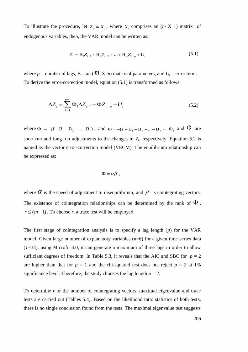
206
To illustrate the procedure, let tt XZ , where
tX comprises an (m X 1) matrix of
endogenous variables, then, the VAR model can be written as:
tptpttt UZZZZ ...2211 (5.1)
where p = number of lags, B = an ( m X m) matrix of parameters, and Ut = error term.
To derive the error-correction model, equation (5.1) is transformed as follows:
tpt
p
l
ltlt UZZZ
1
1
(5.2)
where )...( 21 ll I , and )...( 21 pI . i and are
short-run and long-run adjustments to the changes in Zt, respectively. Equation 5.2 is
named as the vector error-correction model (VECM). The equilibrium relationship can
be expressed as:
' ,
where is the speed of adjustment to disequilibrium, and ' is cointegrating vectors.
The existence of cointegration relationships can be determined by the rank of ,
)1( mr . To choose r, a trace test will be employed.
The first stage of cointegration analysis is to specify a lag length (p) for the VAR
model. Given large number of explanatory variables (n=6) for a given time-series data
(T=34), using Microfit 4.0, it can generate a maximum of three lags in order to allow
sufficient degrees of freedom. In Table 5.3, it reveals that the AIC and SBC for p = 2
are higher than that for p = 1 and the chi-squared test does not reject p = 2 at 1%
significance level. Therefore, the study chooses the lag length p = 2.
To determine r or the number of cointegrating vectors, maximal eigenvalue and trace
tests are carried out (Tables 5.4). Based on the likelihood ratio statistics of both tests,
there is no single conclusion found from the tests. The maximal eigenvalue test suggests

207
that the number of cointegrating vectors is three while the trace test recommends five.
This study chooses r = 3 because, according to Seddighi and Shearing (1997), the
maximal eigenvalue test has greater power than the trace test.
Table 5.3. Test statistics for the length of lags of VAR model
Notes: VAR model is written as tptpttt UZZZZ ...2211, where
tZ = an (m X 1)
matrix of endogenous variables, p = number of lags, B = an ( m X m) matrix of parameters, and Ut =
error term. The chi-squared statistics for p = 3 is not available. * indicates that the chi-squared statistics
are not rejected at 1% significance level.
Table 5.4. Cointegration test
Note: * indicates the rejection of rank (or the number of cointegrating vectors) at 5% significant level.
For the error-correction terms, the first and third cointegrating vectors are statistically
significant (Table 5.5). This indicates that there are two sets of long-run coefficients for
interstate tourism demand. Furthermore, the diagnostic tests reveal that the error-
correction model is correctly specified. Based on the test results in Table 5.5, the
residuals of the model do not have problems of misspecification, serial correlation and
heteroscedasticity. The model also does not reject the null hypothesis of normality.
The signs of long-run coefficients for variables F, DA and OC in Table 5.6 are
consistent with the economic theory. In the long-run, a 1% increase in fuel prices and
Length of
lags (p)
Log likelihood
ratio
Akaike Information
Criterion (AIC)
Schwarz
Bayesian
Criterion (SBC)
Chi-squared statistics
3
712.111
565.111
459.713
NA
2 600.626 502.626 432.361 71.926[0.018]*
1 508.540 459.540 424.408 131.336[0.014]*
0
166.921
166.921
166.921
351.736[0.000]
Rank
Maximal eigenvalue test statistics
5% critical value
Trace test
statistics
5% critical value
r = 0 86.537* 46.470 244.249* 132.450
r = 1 59.617* 40.530 157.712* 102.560
r = 2 38.953* 34.400 98.094* 75.980
r = 3 23.357 28.270 59.141* 53.480 r = 4 15.763 22.040 35.784* 34.870
r = 5 11.570 15.870 20.021 20.180
r = 6
8.451
9.160
8.451
9.160

208
domestic airfares will lead to a decline in interstate tourism demand up to 3.65% and
22%, respectively. On the other hand, given a 1% rise in the price of overseas holidays,
the number of interstate night stays will increase up to 7.17%.
Table 5.5. Error-correction model
Variable
Coefficient
t-ratio
p-value
DIT(-1) -0.146 -1.087 0.289
Y(-1) -3.216* -3.189 0.004
ACC(-1) -1.622* -3.669 0.001
RR(-1) 1.031* 3.266 0.004
F(-1) 0.063 0.275 0.786
DA(-1) 3.140* 3.781 0.001
OC(-1) -0.077 -0.205 0.839
1,1 tZ 0.210* 3.998 0.001
1,2 tZ 0.077 1.467 0.157
1,3 tZ 0.230* 4.368 0.000
Adjusted R2 0.933
Diagnostic tests: Chi-squared p-value
Serial correlation 7.021 0.135
RESET 0.005 0.944 Normality 0.182 0.913
Heteroscedesticity
0.839
0.360
Notes: DIT(-1) = DITt-DITt-1; Y(-1) = Yt-Yt-1; ACC(-1) = ACCt-ACCt-1; RR(-1) = RRt-RRt-1; F(-1) = Ft-Ft-1; DA(-1) = DAt-DAt-1; OC(-1) = OCt-OCt-1; 1, tjZ = error correction term (j = 1, 2 or 3). *
indicates statistical significance at the 1% level of significance for a one-tail test.
However, for accommodation price (ACC), the results are rather mixed. On one hand,
the relationship between interstate tourism demand and ACC does not support economic
theory. The figures in Table 5.6 show that the coefficients of ACC range between +0.93
and +21.08, indicating a rise in accommodation price increases the number of interstate
visitor nights. On the other hand, there is evidence that an increase in ACC could reduce
the visitor nights by 1.05%, which is consistent with the theory.
Furthermore, Table 5.6 also reveals that the long-run coefficients for income and prices
of recreation and restaurants are +47.31 and -34.67, respectively. This indicates that
income and prices of tourism goods and services have significant impacts on the
interstate tourism demand in the long-run. However, this study also finds that the long-

209
run income elasticities can be -0.77. One of the possible explanations is that, even if
household income increases in the long-run, Australian residents will likely to choose
not to travel domestically because it is preferential to use their income for overseas
holidays [Athanasopoulos and Hyndman (2008)]. In addition, the long-run elasticities of
the prices of recreation and restaurants can be +0.84, implying that, to a certain extent,
an increase in the prices of recreation and restaurants will not reduce the number of
night stays by interstate visitors.
A significant limitation of this study is that some of the estimated coefficients are not
consistent with consumer demand theory. A possible reason is that the number of
observations used in this research is small, given that only about 34 observations were
employed, and regressions using small sample size data can yield incorrect inferences
[Lim (2006)]. Therefore, we suggest using panel data analysis in next chapter as this
analysis technique provides larger datasets and degrees of freedom.
Table 5.6. Long-run coefficients for interstate tourism demand
Variable
Cointegrating vector 1 Cointegrating vector 2
Cointegrating vector 3
DIT
-0.191
[-1.000]
-1.625
[-1.000]
-4.959
[-1.000] Y 9.036
[47.313]
-0.357
[-0.220]
-3.809
[-0.768]
ACC 4.025
[21.077]
-1.708
[-1.051]
4.626
[0.933] RR -6.622
[-34.674]
5.458
[3.359]
4.176
[0.842]
F -0.698
[-3.655]
2.410
[1.483]
-2.369
[-0.478] DA -4.198
[-21.981]
-9.166
[-5.641]
-1.498
[-0.302]
OC 1.370
[7.171]
1.122
[0.691]
2.400
[0.484] Intercept -15.498
[-81.153]
-3.062
[-1.884]
32.718
[6.598]
Notes: DIT = Interstate visitor nights; Y = Gross domestic product (GDP) per capita; ACC = Average price of
accommodation per night; RR = Household expenditure on recreation, restaurant and cafes; F = Consumer price
index (CPI) for automotive fuel; DA = CPI for domestic airfare; and OC = CPI of overseas holidays, travel and accommodation. Figures in brackets are normalized value.
Moreover, instead of examining interstate tourism demand in Australia, it is also
worthwhile to examine domestic intrastate and interstate tourism demand in Australia.
According to Tourism Research Australia, domestic tourism in Australia can be
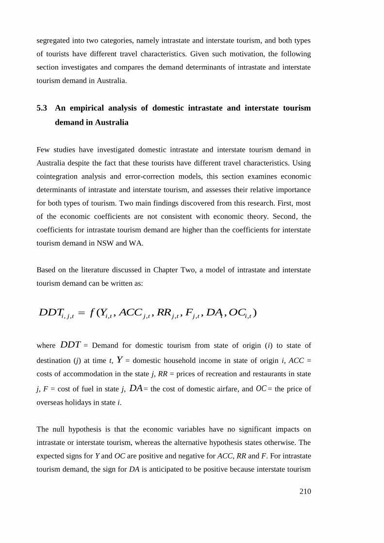
210
segregated into two categories, namely intrastate and interstate tourism, and both types
of tourists have different travel characteristics. Given such motivation, the following
section investigates and compares the demand determinants of intrastate and interstate
tourism demand in Australia.
5.3 An empirical analysis of domestic intrastate and interstate tourism
demand in Australia
Few studies have investigated domestic intrastate and interstate tourism demand in
Australia despite the fact that these tourists have different travel characteristics. Using
cointegration analysis and error-correction models, this section examines economic
determinants of intrastate and interstate tourism, and assesses their relative importance
for both types of tourism. Two main findings discovered from this research. First, most
of the economic coefficients are not consistent with economic theory. Second, the
coefficients for intrastate tourism demand are higher than the coefficients for interstate
tourism demand in NSW and WA.
Based on the literature discussed in Chapter Two, a model of intrastate and interstate
tourism demand can be written as:
),,,,,( ,,,,,,, tittjtjtjtitji OCDAFRRACCYfDDT
where DDT = Demand for domestic tourism from state of origin (i) to state of
destination (j) at time t, Y = domestic household income in state of origin i, ACC =
costs of accommodation in the state j, RR = prices of recreation and restaurants in state
j, F = cost of fuel in state j, DA= the cost of domestic airfare, and OC = the price of
overseas holidays in state i.
The null hypothesis is that the economic variables have no significant impacts on
intrastate or interstate tourism, whereas the alternative hypothesis states otherwise. The
expected signs for Y and OC are positive and negative for ACC, RR and F. For intrastate
tourism demand, the sign for DA is anticipated to be positive because interstate tourism
211
can be a substitute product for intrastate tourism. In other words, an increase in the
airfare for interstate travel will encourage more Australians to travel within their own
states. On the other hand, for interstate tourism, the expected sign of DA is negative,
signifying that a fall in domestic airfares will promote more Australians to travel
interstates.
The data on intrastate tourism demand are based on the number of tourists travelling
within their own states, and for interstate tourism demand, the number of tourists from a
state of origin to a state of destination is used. They are available on quarterly basis
from March 1999 to March 2007 and can be obtained from the Travel by Australians
which is published by Tourism Research Australia. In this research, four states of
destination are employed namely New South Wales, Queensland, Victoria and Western
Australia.
In addition, the data on income and prices of tourism goods and services can be
downloaded from the websites of the Australian Bureau of Statistics and Department of
Transport and Regional Services. The income variable employed in this paper is the
average weekly earnings per person from state of origin. Other potential income
variables such as gross states products have been considered but they are only available
on annual basis. In terms of tourism prices, the average prices of accommodation per
room night and household expenditure on recreation, restaurant and cafes in each state
of destination are used as the proxy variables for the cost of accommodation and price
of recreation and restaurants, respectively. Furthermore, domestic transportation costs
can be measured in terms of the consumer price index (CPI) of automotive fuel in each
state of destination and domestic economy airfares. This study also employs data on
CPI of overseas holidays, travel and accommodation to represent the price of
substituting intrastate and interstate travel. The method used in this study is the
cointegration and error-correction models.
Table 5.7 summarises the empirical analysis of intrastate tourism demand and interstate
visitor arrivals from a state of origin to a state of destination. The results show that
linear models are preferred in only 28% of the cases. In addition, not all interstate
tourism demand data have long-run relationships with the economic determinants. The
error-correction terms for interstate visitor arrivals from Queensland (QLD) to New

212
South Wales (NSW), Tasmania (TAS) to NSW and Western Australia (WA) to QLD
are not statistically significant at 5% level. In terms of diagnostic testing on the error-
correction models, the null hypotheses of the tests are not rejected by all interstate and
intrastate tourism demand data, except for the data on interstate visitor arrivals from
South Australia (SA) to Victoria (VIC) and WA.
Table 5.8 provides the short-run coefficients for those variables that are statistically
significant at 5% level. The results reveal that the changes in all economic variables,
except income, affect interstate tourist arrivals to QLD in the short-run. Furthermore,
domestic household income has a significant short-run effect on tourist arrivals from
VIC to NSW. Another remarkable finding in Table 5.8 is that the changes in domestic
airfares in the short-run can strongly influence the demand for intrastate tourism in WA.
In terms of economic effects on intrastate and interstate tourism demand in the long-run,
this study finds that a large number of long-run economic coefficients are not consistent
with economic theory (Table 5.9). For instance, the signs of domestic airfares variables
for interstate tourist arrivals to NSW are positive. Similarly, there is a positive long-run
relationship between fuel price and interstate tourist arrivals to QLD. Furthermore, most
of the signs of income coefficients for intrastate and interstate tourism demand are
negative, indicating that an increase in domestic household income will lead to a decline
in both components of tourism demand. These results are supported by Athanasopoulos
and Hyndman (2008), who argue that, when the domestic household income increases,
Australian residents will likely choose not to travel domestically but travel overseas
instead.
Nevertheless, this study found that several estimates have the expected signs. Table 5.9
reveals that the signs of the RR and domestic airfares coefficients are negative for
interstate tourist arrivals to VIC, implying that an increase in the costs of recreation and
restaurants and domestic airfares in the long-run can cause a decrease in the number of
interstate tourists in VIC. Similarly, this study discovers that a rise in the cost of fuel
and domestic airfares will have negative impact on interstate tourist arrivals to WA.
Overall, it is apparent that domestic transportation costs are important determinants for
interstate tourist arrivals to VIC and WA.

213

214
Table 5.7. A summary results of model specification, the significance of error
correction term and diagnostic tests
State of
destination
State of
origin
Functional
form
specification
Lag of
VAR
model
The significance of
error-correction term
at 5% level
Rejection of the
null hypotheses of
the diagnostic tests
NSW ACT Linear 1 YES NO
QLD Log-linear 3 NO NO
NT Log-linear 1 YES NO
SA Log-linear 1 YES NO
TAS Log-linear 1 NO NO
VIC Log-linear 3 YES NO
WA Linear 1 YES NO
Intrastate Linear 1 YES NO
QLD ACT Linear 2 YES NO
NSW Log-linear 3 YES NO
NT Log-linear 1 YES NO
SA Log-linear 3 YES NO
TAS Log-linear 1 YES NO
VIC Log-linear 3 YES NO
WA Log-linear 3 NO NO
Intrastate Log-linear 1 YES NO
VIC ACT Log-linear 3 YES NO
NSW Log-linear 3 YES NO
NT Linear 3 YES NO
QLD Log-linear 1 YES NO
SA Linear 3 NO YES*
TAS Log-linear 1 YES NO
WA Log-linear 3 YES NO
Intrastate Log-linear 3 YES NO
WA ACT Linear 3 YES NO
NSW Log-linear 3 YES NO
NT Log-linear 1 YES NO
QLD Log-linear 1 YES NO
SA Linear 3 NO YES*
TAS Log-linear 3 YES NO
VIC Log-linear 1 YES NO
Intrastate Linear 3 YES NO
Note: ACT= Australian Capital Territory; NSW=New South Wales; NT=Northern Territory;
QLD=Queensland; SA=South Australia; TAS=Tasmania; VIC=Victoria; WA=Western Australia. *Even
after transformed from log-linear to linear models, the latter models still encounter the problems of model
misspecification. The results for interstate tourist arrivals from SA to VIC and WA are not reliable, and
hence, we choose not to disclose the results.

215
Table 5.8. Estimated short-run coefficients
State of
destination
State of
origin
Estimated coefficients
d(DDT1) d(DDT2) d(Y1) d(ACC1) d(ACC2) d(RR1) d(RR2) d(RR3) d(F1) d(F2) d(DA1) d(DA2) d(OC1) d(OC2)
NSW VIC 4.607 -1.350 4.592
1.562 0.585 1.488
QLD ACT -1.913 3.793
0.688 1.311
NSW 0.974 4.850 -2.887 -1.275 -1.545 -0.978 -1.869 -1.535
0.298 1.104 0.641 0.442 0.462 0.394 0.822 0.579
VIC 0.825 4.129 -1.893
0.326 1.736 0.734
VIC ACT -3.895
1.685
NSW 4.986
1.887
NT 0.867 0.401
0.279 0.148
Intrastate 1.368
0.588
WA TAS 0.804 -7.717 -5.920
0.322 2.875 2.174
Intrastate -40.129
15.876
Note: d(Zt)=Zt – Zt-1, where d= difference, Z = economic variable, and t = time. DDT=demand for intrastate or interstate tourism; Y=domestic income; ACC=the cost of accommodation; RR=the price
of recreation and restaurants; F=fuel price; DA=domestic airfares; OC=the price of overseas holidays. The two entries corresponding to each variables are their estimates (in bold) and standard errors,
respectively. The above figures are statistically significant at 5%. Non-significant variables are not reported here.

216
By comparing the effects of economic variables on intrastate and interstate tourism
demand, this study revealed mixed results. For NSW and WA, the long-run economic
coefficients for intrastate tourism demand are higher than the coefficients for interstate
tourism demand (Table 5.9). This indicates that, in the long-run, changes in domestic
household income and tourism prices will have a stronger influence on the demand for
intrastate tourism than interstate tourism in NSW and WA. However, Table 5.9 exhibits
different perspectives for QLD and VIC. When fluctuations in income and tourism
prices occur, the long-run impacts on intrastate and interstate tourism demand are
relatively similar for QLD and VIC.
In general, this study suggests that NSW and WA State Governments need to consider
the facts that changes in economic conditions will have a stronger influence on the
demand for intrastate tourism than interstate tourism in NSW and WA. Hence, in the
light of planning effective marketing strategies, NSW and WA State Governments
should develop separate intrastate and interstate tourism policies. However, based on
the findings of this study, separate intrastate and interstate tourism policies may not be
useful for promoting tourism in QLD and VIC.
Despite the above findings, there is a limitation in this research. Most of the long-run
economic coefficients are not consistent with the prior expectations. This issue could be
caused by the small sample size dataset. To overcome such an issue, using panel data
analysis may be useful.
5.4 Conclusion
In the early research of Australian domestic tourism demand, Hamal (1996) argued that,
to obtain reliable estimations using cointegration analysis, it would be ideal if a larger
sample size is used. In Hamal‟s research, the author used 18 time-series observations. In
this current research, approximately 40 time-series data points were employed, in which
the data was available and provided by Tourism Research Australia.
In this chapter, two types of research have been carried out. The first research was to
investigate domestic interstate tourism demand in Australia. The second research was

217
Table 5.9. Estimated long-run coefficients
State of
destination
State of
origin
Estimated coefficient
Y ACC RR F DA OC
NSW ACT 0.120 -1.329 -0.013 -0.631 2.088 -0.026
NT -0.596 -12.282 8.296 0.5072 3.104 -5.249
SA -2.773 -2.861 -0.447 1.114 5.249 0.762
VIC -0.769 2.618 -1.235 -1.960 5.198 2.323
WA -1.206 6.164 -0.007 -0.436 12.851 2.908
Intrastate -51.288 -134.383 3.679 -1.941 167.623 -36.294
QLD ACT 0.056 1.140 0.007 -0.182 -3.188 -0.397
NSW 1.868 -1.782 0.793 0.336 0.396 0.778
NT -0.919 -6.845 19.943 3.115 36.030 9.282
SA -42.833 1.422 -1.969 14.061 9.734 12.453
TAS 2.763 -5.462 2.629 0.208 7.516 -2.578
VIC 0.4670 -0.795 0.977 0.568 -3.029 0.043
Intrastate 4.794 0.319 -1.318 -0.410 -4.630 -0.255
VIC ACT 3.515 6.319 -3.522 -2.896 0.433 0.337
NSW -0.186 -2.422 -1.258 -0.282 -1.089 -1.170
NT -0.110 -0.724 -0.005 -0.174 -0.860 -0.016
QLD 3.579 1.688 -0.910 0.918 -8.708 0.527
TAS 5.195 7.783 -3.778 -1.015 -7.613 1.018
WA 2.420 -0.338 -0.501 0.838 -3.208 -0.687
Intrastate -0.386 1.867 0.049 -0.183 -2.520 0.546
WA ACT 1.030 7.066 -0.326 -2.555 -4.943 0.764
NSW -12.478 -1.373 3.123 14.510 -34.180 5.751
NT -33.753 -15.512 -11.852 -13.025 -21.805 -13.823
QLD 15.322 1.187 -1.914 -0.179 -4.264 0.639
TAS 4.520 14.890 -8.103 -0.470 -8.378 -0.979
VIC 3.914 1.354 -8.771 -1.071 -8.336 -9.005
Intrastate -11.369 60.197 0.527 -4.787 66.998 24.285
Note: The long-run coefficients for interstate tourist arrivals from QLD to NSW, WA to QLD, SA to VIC
and SA to WA are not significant. Hence, they are not reported in this paper. Figures in BOLD denote the
coefficients that are not consistent with economic theory.

218
the extension of the first one, where domestic intrastate tourism demand was
incorporated. Both studies applied consumer demand theory and used a cointegration
analysis to generate the demand estimations. Diagnostic tests were used to examine the
existence of misspecification problems.
Not all results obtained from both researches were consistent with the theory. In certain
cases, the coefficient signs were contradictory with prior expectations. One of the
possible reasons is that the number of observations used in both studies was small, even
though the sample size has increased compared to Hamal‟s research. Based on the
results, we proposed that using a panel data methodology would be useful. This method
combines cross-section and time-series data, which provides larger datasets and degrees
of freedom [Song and Witt (2000)].
Given this, the following chapter replicates the above studies by using panel data
analysis.
219
Chapter 6
Modelling Australian domestic tourism
demand (II): A panel data analysis
6.1 Motivation
In Chapter Two, a discussion about income, tourism prices and other leading economic
variables and the theoretical frameworks for modelling tourism demand was carried out.
Following on from that, using cointegration analysis, the empirical research referred to
in Chapter Five shows robust evidence that income and tourism prices are the important
determinants of Australian domestic tourism demand. However, in some cases, the
analysis failed to generate the coefficient signs that are consistent with consumer
demand theory. This issue could be related to the small sample size dataset used. Hence,
to overcome this problem, a panel data analysis is employed in this chapter to model
Australian domestic tourism demand.
6.2 Estimation of Australian domestic tourism demand
According to consumer demand theory which was discussed in Chapter Two, domestic
tourism demand can be written (in panel data format) as:
),,,,( jtjtjtjtjtjt DUMOCTCTPYfTD
where TD = Demand for domestic tourism at time t in State j, Y = domestic household
income, TP = tourism prices, TC = transportation costs , OC = the price of overseas
holidays and DUM = dummy variable for one-off events (such as the Bali bombings in
2005 and the Sydney Olympic Games in 2000) and seasonality. According to the
literature, the expected signs of TP and TC are negative, whereas OC would be
anticipated to have a positive sign. For Y, it can be either positive or negative. For the
dummy variables, it would depend on the nature of the one-off events. For instance,
global unfavourable events such as Bali bombings and the outbreak of SARS would
220
encourage Australians to travel within their own country. Hence, the dummy variables
for these negative events would have a positive sign.
Unlike the cointegration analysis where pure time-series data with approximately 40
observations was used, this chapter employs pooled data which are based on seven
Australia States from 1999 quarter 1 to 2007 quarter 4. This provides a total of 252
pooled observations.
This thesis uses numbers of domestic overnight visitors and visitor nights in Australia as
the dependent variables for Australian domestic tourism demand. In the tourism
literature, Faulkner (1988) highlighted that statistics based on visitor nights are
significant from an economic viewpoint because they reflect the utilisation of tourism
facilities and related tourism expenditure. However, the data on visitor nights suffers
from large sampling variability (Travel by Australians, Quarterly report 1998-2006).
For this reason, the number of overnight visitors will also be used.
Furthermore, disaggregate data is employed rather than aggregate data because the
former contains more information about the nature of the tourists. Furthermore, Kim
and Moosa (2005) found that forecasting using disaggregate data generates more
accurate forecasts than using aggregate data. Therefore, in this chapter, we use six types
of domestic tourism demand data, namely the numbers of visitor nights by holiday-
makers (HOL), business visitor nights (BUS), visitors of friends and relatives (VFR),
other purpose of visits (OTH), interstate and intrastate visitors. In addition, another two
types of data are employed, namely the number of interstate and intrastate overnight
visitors.
For the independent variables, several variables are used as a proxy for household
income. They are disposable income, gross domestic product (GDP) and GDP per
capita. On the other hand, the CPI for domestic holidays and accommodation is used as
a proxy for tourism prices. It represents the aggregate prices of domestic travel in
Australia. As for transportation costs, the proxy variables are the CPI for automotive
fuel.

221
All dependent and explanatory variables are summarised in Table 6.1. All variables are
expressed in logarithms. The logarithm data is used in this study because the functional
form can be specified in log-linear model. According to Lim (1997), such model is
widely employed in tourism demand research because the coefficients can be expressed
as elasticities. Unfortunately, it seems that no functional form test is available at this
stage for panel data. Hence, this thesis uses logarithm data to generate elasticity
coefficients for the convenience of interpreting the results.
Table 6.1. List of proxy variables
Proxy variables Notation Proxy for: Source of
data*
Definition and the rational
explanation of using this proxy
variable CPI for
automotive fuel
F Transportation
costs ABS Definition: The average price of
unleaded petrol, premium
unleaded petrol, diesel and LPG. The variable is a proxy for the
cost of travel. This variable has
been used by Hultkrantz (1995)
to model domestic tourism
demand in Sweden.
CPI for
domestic
holidays and
accommodation
DT Tourism
prices ABS Definition: The average price
based on the aggregation of air,
sea and rail travel, car hire, hotel
and motel accommodation and
package travel for domestic
holidays in Australia. As the price index increases, the
demand for domestic tourism is
expected to decline, vice versa
when the price decreases.
CPI for overseas
holidays and
accommodation
OC Price of
overseas
holidays
ABS Definition: A measure of prices
charged on air, sea and rail travel,
car hire, hotel and motel
accommodation and package
travel for overseas holidays. As overseas travel is a substitute
product for domestic holidays, an
increase in the price index of
overseas travel will lead to an
increase in domestic tourism
demand.
Disposable
income DI Household
income ABS and
RBA Definition: The balance of
household income after deducted
all household expenditure. This variable is highly suggested

222
Proxy variables Notation Proxy for: Source of
data*
Definition and the rational
explanation of using this proxy
variable by Lim (1997 and 2006) because
it represents the amount of
money which can be spent for
leisure and recreation purposes.
Gross domestic
product GDP Household
income ABS Definition: A measure of
production for the economy as a
whole. In international tourism demand
literature, this variable has been
widely used as a proxy for
tourists‟ income [Lim (2006)]. In
this study, the intention is to
examine whether an increase in
Australia‟s economic growth can
lead to a rise in domestic tourism
demand.
GDP per capita GDPP Household
income ABS Definition: A measure of the
consumer‟s wealth in Australia. It represents the household
income level for each resident in
Australia.
Numbers of : (1)
interstate visitor
nights, (2)
intrastate visitor
nights, (3)
interstate
visitors, and (4)
intrastate
visitors
(1) NV
(2) NVI
(3) OV
(4) OVI
Domestic
tourism
demand
TRA Definition: It is collected based
on how many domestic visitors
who travel within their own state
and interstate. Visitor nights are
measured as the number of nights
stayed in a state. The data on visitor numbers and
nights have been widely
employed as proxy variables for
international tourism demand
[Lim (1997)]. This research will
employ similar type of data in the
context of intrastate and
interstate tourism demand.
Numbers of
visitor nights by
purpose of
visits, namely: (1) Holiday
(2) Business
(3) Visiting
friends and
relatives
(1) HOL
(2) BUS
(3) VFR
(4) OTH
Domestic
tourism
demand
TRA Definition: The variable
measures the number of visitor
nights by four main types of
tourists, namely tourists who are
holiday-makers, business
purpose, visiting friends and
relatives, and others (i.e.
education and working holidays). This variable is commonly used
for evaluating the effects of
income and tourism prices
changes on different types of

223
Proxy variables Notation Proxy for: Source of
data*
Definition and the rational
explanation of using this proxy
variable
(4) Others
domestic tourists. It has been
employed in Athanasopoulos and
Hyndman (2008).
*TRA stands for Tourism Research Australia; ABS stands for the Australian Bureau of
Statistics; RBA stands for the Research Bank of Australia; DOTARS stands for the
Department of Transport and Regional Services.
6.3 Panel unit root tests
In a panel data analysis, it is crucial to investigate whether the pooled data is stationary
or not. Baltagi (2001) asserted that, as the number of cross-section units and length of
time-series increases, it is imperative to determine asymptotic properties of panel OLS
estimations and to ensure stationary of panel data.
For this research, an IPS unit root test is employed. The test is developed by Im, Pesaran
and Shin (2003) which allows for individual unit root process to vary across all cross-
sections [Eviews (2007)]. In the tourism literature, Narayan (2006) used this test to
examine international tourist arrival to Australia.
To illustrate that, a panel Augmented Dickey-Fuller (ADF) regression is written as
follows:
jt
p
l
jjljtjljtjt utYyYi
1
1 (6.1)
where jtY = a panel data with individuals j = 1,2,...,N and time-series observations t =
1,2,...,T , j = unit-specific fixed effects, t = time trend, j = coefficients of time-trend
and jtu = error term. Unlike the pure time-series ADF test, the auxiliary equation (6.1)
contains unit-specific fixed effects which allow for heterogeneity across cross-section
data [Asteriou and Hall (2007)].

224
For the IPS test, it allows heterogeneity on φ and runs the auxiliary regression (6.1)
based on the average of the individual unit root test statistics [Im et al (2003) and
Asteriou and Hall (2007)]. To illustrate that, the hypotheses of IPS test are written as
follows:
0: jHo for all j
0:1 jH , j = 1,2,...,N1 and 0i , j = N1+1,N1+2,...,N.
The null hypothesis states that all cross-section series are non-stationary whereas under
the alternative hypothesis, a part of the total series in the panel is stationary. For the IPS
test, Im et al. (2003) constructed a t-statistic which the null hypothesis follows the
standard normal distribution as T (and subsequently N) approaches to infinity.
The results of the panel unit root tests in Table 6.2 consist of two auxiliary regressions,
in which one with intercept and without trend, and another with an intercept and a trend.
Based on the table, it is found that there are no unit root problems in the logarithm and
first differenced panel data for all types of dependent variables.
On the other hand, for independent variables, Table 6.3 shows that the IPS test rejects
the null hypothesis for the DI and DT level data, indicating that these variables are
stationary in panels. In contrast, the test does not reject the null hypothesis for the F,
GDP, GDPP and OC level data. After taking first-differencing on all variables, all
independent variables become stationary, except for GDP. Nevertheless, the GDP
variable becomes stationary when the auxiliary regression included a trend. Overall, this
concludes that the panel data for F, GDP, GDPP and OC variables are I(1), whereas the
panel data for DI and DT are I(0).
In conclusion, the IPS test found that four out of six variables are I(1) when logarithm
data are tested and I(O) after first-differenced the data. Hence, to ensure data stationary
for all variables, this thesis uses first-difference data. Furthermore, by differencing the
data and removing the problem of potentially non-stationary observations, panel data
analysis will give us confidence in the reported coefficients and standard errors [Garin-

225
Munoz (2007)]. Given this, the following panel data estimations are based on first
differenced pooled data (or percentage growth panel data).
Table 6.2. IPS panel unit root test for the dependent variables
Panel data Auxiliary regression
specification Level First-differenced
BUS No trend -5.036 -18.998
Trend -10.106 -18.109
HOL No trend -10.178 -34.304
Trend -9.368 -27.761
VFR No trend -6.185 -24.156
Trend -5.176 -23.792
OTH No trend -14.982 -17.293
Trend -13.923 -17.199
NV No trend -7.490 -21.642
Trend -12.651 -21.136
NVI No trend -4.569 -13.800
Trend -11.565 -12.941
OV No trend -4.120 -18.397
Trend -10.904 -17.384
OVI No trend -3.491 -25.163
Trend -4.588 -24.701
Note: BUS = number of business visitor nights, HOL = number of holiday visitor nights, VFR =
number of nights by visitors friends and relatives, OTH = number of nights by visitors with
other visiting purpose, NV = number of night visited by domestic interstate visitors, NVI =
number of night visited by domestic intrastate visitors, OV = number of domestic overnight
interstate visitors, and OVI = number of domestic overnight intrastate visitors. All data are
expressed in logarithm. The null hypothesis of all above panel unit root tests is that the panel
data are not stationary. The auxiliary regression is specified with an intercept and a trend in all
tests. The IPS tests use t-statistics [Refer to Im et al. (2003) for more details]. The critical values
for the regression without a trend at the 1%, 5% and 10% significance levels are -2.29, -2.07
and -1.95, respectively. The critical values for the regression with a trend at the 1%, 5% and
10% significance levels are -2.90, -2.68 and -2.57, respectively.
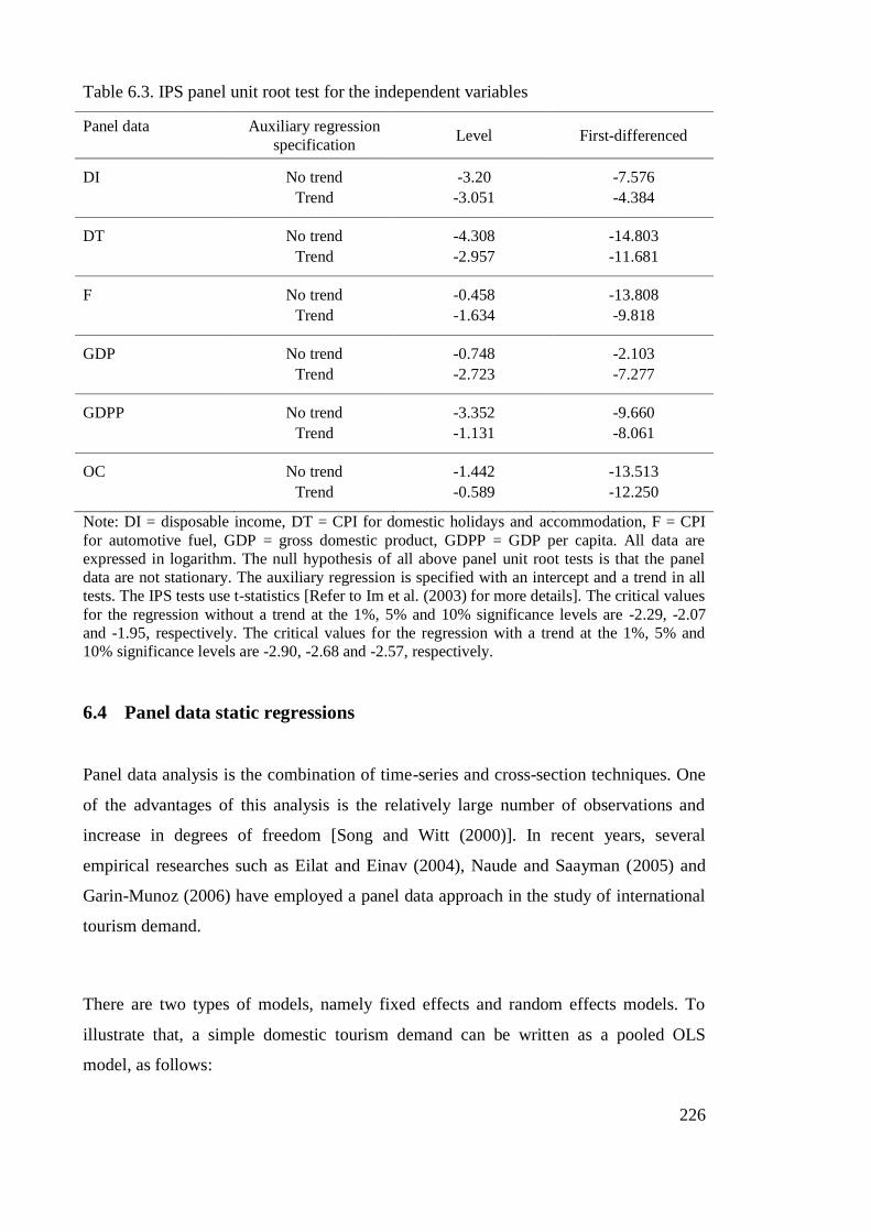
226
Table 6.3. IPS panel unit root test for the independent variables
Panel data Auxiliary regression
specification Level First-differenced
DI No trend -3.20 -7.576
Trend -3.051 -4.384
DT No trend -4.308 -14.803
Trend -2.957 -11.681
F No trend -0.458 -13.808
Trend -1.634 -9.818
GDP No trend -0.748 -2.103
Trend -2.723 -7.277
GDPP No trend -3.352 -9.660
Trend -1.131 -8.061
OC No trend -1.442 -13.513
Trend -0.589 -12.250
Note: DI = disposable income, DT = CPI for domestic holidays and accommodation, F = CPI
for automotive fuel, GDP = gross domestic product, GDPP = GDP per capita. All data are
expressed in logarithm. The null hypothesis of all above panel unit root tests is that the panel
data are not stationary. The auxiliary regression is specified with an intercept and a trend in all
tests. The IPS tests use t-statistics [Refer to Im et al. (2003) for more details]. The critical values
for the regression without a trend at the 1%, 5% and 10% significance levels are -2.29, -2.07
and -1.95, respectively. The critical values for the regression with a trend at the 1%, 5% and
10% significance levels are -2.90, -2.68 and -2.57, respectively.
6.4 Panel data static regressions
Panel data analysis is the combination of time-series and cross-section techniques. One
of the advantages of this analysis is the relatively large number of observations and
increase in degrees of freedom [Song and Witt (2000)]. In recent years, several
empirical researches such as Eilat and Einav (2004), Naude and Saayman (2005) and
Garin-Munoz (2006) have employed a panel data approach in the study of international
tourism demand.
There are two types of models, namely fixed effects and random effects models. To
illustrate that, a simple domestic tourism demand can be written as a pooled OLS
model, as follows:

227
jtjjtjt vcy (6.2)
where:
jty = demand for domestic tourism in State j
c = a common constant term
v = a vector of explanatory variables.
t = time subscript.
j = individual-specific effect of each State j
= a coefficient matrix
𝜂 = error term.
Estimating equation 6.2 could be problematic because including many j can cause
dummy variable trap or perfect multicollinearity. Hence, to avoid such issue, Baltagi
(2008) developed a regression that averages the regression 6.2 over time. The regression
is expressed as follows:
jjjj vcy (6.3)
where y = mean value of domestic tourism demand data, v = mean value of the
explanatory variables, and = mean of error terms. Thereafter, by subtracting (6.3)
from (6.2), it is written as:
)()( jjtjjtjjt vvyy (6.4)
or *** ' jtjtjt vy ,
where *
jty = jjt yy , *' jtv = )( jj vv ,
*
jt = )( jjt and
𝛼𝑖𝑗𝑖=1 = 0
Equation 6.4 is called a fixed effects model.

228
Nevertheless, the model suffers from losing a number of degrees of freedom. According
to Gujarati (2003), if equation (6.2) includes too many j , then the degrees of freedom
will decline.
Hence, to tackle this issue, a random effects model is introduced. Unlike the fixed
effects model which incorporates the individual-specific effects as dummy variables, the
random effect model treats the effects as error components. It is written as follows:
jtjtjt vy ' (6.5)
where jtv = a matrix of explanatory variables, = coefficient matrix. The error term of
equation (6.5) is jtjjt u , where uj = individual-specific error component and jt =
errors from different cross-section units. Equation (6.5) assumes that jtv are
uncorrelated with jt . OLS estimation of this model is asymptotically unbiased, but it
can generate inefficient standard errors.
To determine the appropriate models for modelling domestic tourism demand, the
Hausman Specification (HS) tests will be carried out. The test examines whether j are
correlated withjtv . If the null hypothesis (Ho:
j are not correlated withjtv ) is not
rejected, it indicates that both estimates of fixed and random effects models are
consistent. In other words, there is no difference between the estimations of both
models. Conversely, if the HS test rejects the null hypothesis, this implies that the fixed
effects estimator is consistent but not the random effects model [Romilly et al. (1998)
and Johnston and DiNardo (1997)].
The fixed-effects model shown in regression (6.4) assumes homoskedasticity in the
residuals. According to Baltagi (2001), this is a restrictive assumption for panel data
models. Cross-section heteroskedasticity may exist because cross-sectional units may be
of varying size and exhibit different variation. To take accounts of heteroscedasticity
effects in panel data regressions, generalised least square (GLS) models are introduced.

229
To tackle cross-section heteroskedasticity, the OLS estimations in the panel data models
have to be transformed into GLS estimations in order to obtain unbiased and efficient
estimates. For example, the OLS estimates of in equations (6.5) are given as follows:
N
j
jj
N
j
jjOLS yVVV1
'
1
1
'
where '
2,1 ),...,( jTjjj vvvV and N = the number of cross-section units. According to
Arellano (2003), the above OLS estimate is unbiased and consistent but inefficient.
Hence, the optimal estimation can be achieved through the GLS transformation, which
is expressed as follows:
N
j
jj
N
j
jjGLS yVVV1
1'
1
1
1' (6.6)
where )( jjE . This GLS estimator is not feasible as is unknown. However, in
Eviews 6.0, we can estimate fixed effects model using feasible GLS coefficients by
generating a series of estimated residuals and then use these residuals for estimating
weighted least squares. Further mathematical derivations of feasible GLS can be found
in Arellano (2003) and Baltagi (2001). For convenience, we name the fixed-effects
model which is cross-sectional heteroscedascity adjusted, as FE-CSH.
Another method of analysing panel data is to use seemingly unrelated regression
estimation. It assumes that the errors are correlated across cross-section units but
independent over time [Eviews (2007)]. According to Maddala (2001), this type of
correlation would arise if there are omitted variables which are common to all
equations. To conduct SUR estimation in a GLS method (hereafter named as FE-SUR),
the GLS coefficient is similar to (6.6) but the difference is that )( ljE where
lj .
All estimations using the panel data static models are summarised in Tables 6.4 – 6.11.
Note that, the ACC and RR appear in time-series cointegration analysis (Chapter 5) are

230
found to be statistically significant. However, when the panel data for ACC and RR
variables are used, the ACC and RR are statistically insignificant. Therefore, these
variables are excluded from panel data analysis (Chapter 6). Instead, CPI for domestic
holidays and accommodation (DT) is used to replace ACC and RR as a proxy variable
for tourism prices. Similarly, as the CPI for overseas holidays and accommodation is
found to be statistically insignificant in all cases, we decided to omit this variable from
this study.
The effects of income changes on domestic travel are distinct from one type of visitors
to another. On one hand, the income variables for holiday and business visitor nights are
highly elastic and positive. On the other hand, the income variables are shown as
negative for VFR, OTH and interstate tourism data. For instance, in Table 6.4, the
GDPP(-1) estimate for holiday visitor night data is 8.56, suggesting that Australians
tend to travel more domestically for holiday purposes when their household income
increases. As the estimated elasticity is high and exceeded one, domestic holiday trips
can be regarded as a luxury trip. Similarly, the GDP and GDPP(-1) coefficients for
business visitor night data are 1.12 and 11.1, respectively, showing that the demand for
domestic business tourism is strongly responsive to the conditions of Australian
economy (See Table 6.5). Conversely, the disposable income coefficients for domestic
VFR visitor night data range between -0.70 and -1.18 (See Table 6.6), whilst the GDPP
coefficient for interstate visitor data range between -3.42 and -6.97 (See Tables 6.8 and
6.10). This means that a growth in disposable income will cause Australian households
to forego domestic VFR and interstate trips, and alternatively, may choose overseas
travel or purchase other luxury household products.
With regard to the tourism prices, only the CPI of domestic travel (DT) and automotive
fuel (F) variables are found to be statistically significant in this current research.
Accordingly, the estimates for one-period-lagged domestic tourism prices [DT(-1)] and
two-period-lagged domestic tourism prices [DT(-2)] are negative and statistically
significant for most types of domestic tourism data. This implies that an increase in
current tourism prices will lead to a fall in domestic tourism demand in the next one and
two quarters (See Tables 6.4 – 6.11). Moreover, this study also discovers that the
DT(-1) coefficients are considerably high (ranging from -0.49 to -3.06), but this is
somewhat lower that the DT(-2) estimates (ranging from -0.59 to -7.10). To put it

231
differently, those Australian households who plan their domestic trips two-quarters
ahead are more responsive to price changes than those who plan a quarter ahead. In
addition, for OTH visitor night data, the coefficient for F is -1.3, indicating that an
increase in current fuel prices will have an inverse effect on „other‟ visitor travel.
The incidents of the Bali bombings have influences on the demand for holiday, VFR,
interstate and intrastate trips. Furthermore, the coefficients for Bali have a positive sign
for all cases, suggesting that Australians would substitute from overseas travel (Bali) to
domestic trips when Bali bombings incidences occurred. Nevertheless, as most of the
coefficients are below one, this means that the influences of Bali bombing incidences on
Australian domestic tourism demand are not strong.
This study also reports that seasonality exists in Australian domestic tourism demand.
Seasonal dummy variables are shown as significant for all types of domestic visitors,
except for the business visitor night data. This implies that domestic tourists travel
mostly during summer school holidays in January and mid-term school holidays in July.
Apart from that, the F-statistics reject the null hypothesis of δ1= δ2=...= δn=0 at the 1%
significance level for most cases, indicating that all independent variables are important
in explaining all types of domestic tourism demand data. However, the only exception is
when using FE-SUR in modelling interstate tourism demand (See Table 6.10).
Accordingly, the F-test cannot reject the null hypothesis at the 10% significance level,
indicating that the independent variables are not jointly significant using the FE-SUR
model.
The random effects estimations show relatively similar results to the fixed effects
regression results. Based on the Hausman test, they do not reject the null hypothesis that
j are not correlated withjtv . In other words, the choice between the fixed and random
effects models is indifferent because the estimates from both models are consistent.
Nevertheless, note that the chi-squares statistics for the Hausman test are zero and this is
not unusual because the estimations for the fixed and random effects models are not
significantly different from each other [Johnston and DiNardo (1997)].

232
Table 6.4. Estimate of the double-log static panel model [Dependent variable: Holiday
visitor nights (HOL)]
Coefficients Panel models
Fixed effects FE-CSH FE-SUR Random effects
Constant
-0.149***
(0.043)
GDPP(-1)
8.564**
(3.516)
DT(-1) -3.057*** -0.965** -1.833*** -3.040***
(1.033) (0.458) (0.485) (1.040)
DT(-2) -7.010*** -2.092*** -3.40*** -6.972***
(1.036) (0.391) (0.544) (1.035)
Bali 0.212* 0.10*** 0.078* 0.211**
(0.092) (0.026) (0.043) (0.091)
S1 0.749*** 0.532*** 0.539*** 0.747***
(0.118) (0.048) (0.052) (0.118)
S2 0.223** -0.199*** -0.062 0.221**
(0.105) (0.036) (0.058) (0.102)
W(δ1=δ2=...=δn= 0) 9.128*** 21.563*** 9.666*** 20.551***
𝜂
4.663E-15
1.776E-14
0
1.532E-14
Hausman test 0.000
Prob(Hausman
test) 1.000
Note: The research uses four types of panel models, namely fixed effects, panel cross-section
heteroscedesticity (FE-CSH), panel seemingly unrelated regression (FE-SUR) and random effects
models. The dependent and independent variables are based on log-differenced data. Figures in brackets
are the White cross-section standard errors, respectively. Bali = dummy variable for bombing incidents in
Bali; DT(-1) = one-quarter lagged CPI of domestic travel; DT(-2) = two-quarters lagged CPI of domestic
travel; GDPP(-1) = one-quarter lagged GDPP; S1 = seasonal dummy from January to March; S2 =
seasonal dummy from April to June. F-statistics is used to test Ho: δ1= δ2=...= δn= 0. 𝜂 denotes the
value of the residuals determinant. The Hausman test is to examine whether the estimations of random
effect models are similar to the estimations of fixed effects models. ***, **, * denotes significant at 1%,
5% and 10% levels, respectively.

233
Table 6.5. Estimate of the double-log static panel model [Dependent variable: Business
visitor nights (BUS)]
Coefficients Panel models
Fixed effects FE-CSH FE-SUR Random effects
Constant
-0.062*
(0.032)
GDP 1.122**
1.010** 1.122**
(0.514)
(0.480) (0.508)
GDPP(-1) 11.096** 9.276* 8.905** 11.096**
(4.894) (4.934) (4.503) (4.829)
DT(-1) -1.414* -1.304** -1.398** -1.413*
(0.728) (0.618) (0.627) (0.718)
W(δ1=δ2=...=δn= 0) 3.257*** 2.857*** 2.731*** 9.947***
𝜂
2.165E-15
1.887E-15
3.331E-15
4.496E-15
Hausman test 0.000
Prob(Hausman
test) 1.000
Note: The research uses four types of panel models, namely fixed effects, panel cross-section
heteroscedesticity (FE-CSH), panel seemingly unrelated regression (FE-SUR) and random effects
models. The dependent and independent variables are based on log-differenced data. Figures in brackets
are the White cross-section standard errors, respectively. DT(-1) = one-quarter lagged CPI of domestic
travel; GDP = gross domestic product; GDPP(-1) = one-quarter lagged GDPP. F-statistics is used to test
Ho: δ1= δ2=...= δn= 0. 𝜂 denotes the value of the residuals determinant. The Hausman test is to
examine whether the estimations of random effect models are similar to the estimations of fixed effects
models. ***, **, * denotes significant at 1%, 5% and 10% levels, respectively.
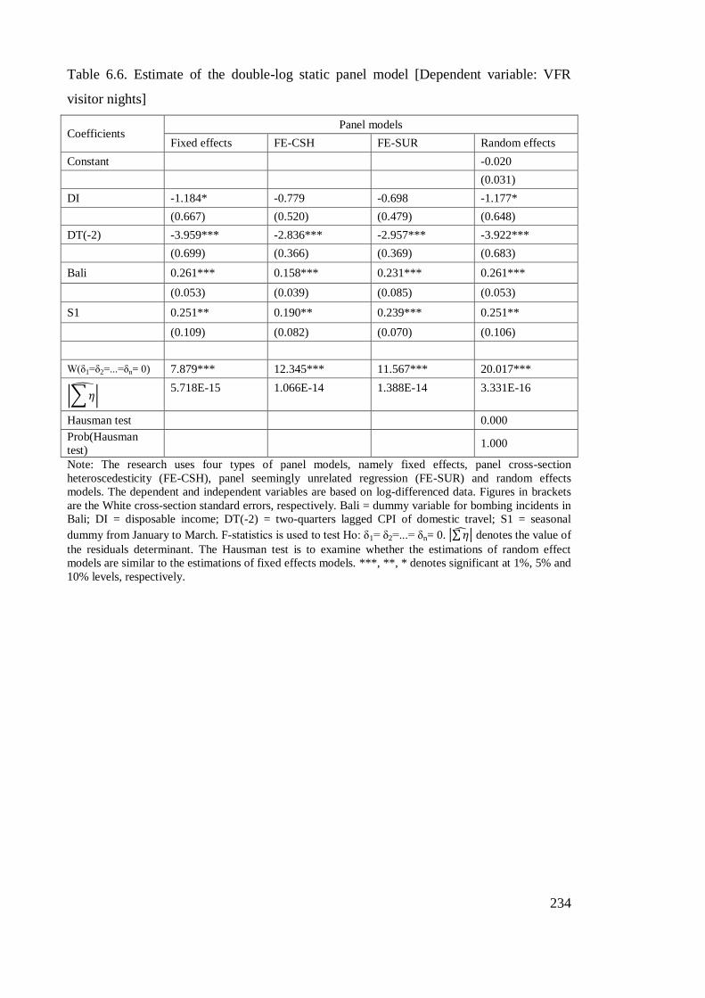
234
Table 6.6. Estimate of the double-log static panel model [Dependent variable: VFR
visitor nights]
Coefficients Panel models
Fixed effects FE-CSH FE-SUR Random effects
Constant
-0.020
(0.031)
DI -1.184* -0.779 -0.698 -1.177*
(0.667) (0.520) (0.479) (0.648)
DT(-2) -3.959*** -2.836*** -2.957*** -3.922***
(0.699) (0.366) (0.369) (0.683)
Bali 0.261*** 0.158*** 0.231*** 0.261***
(0.053) (0.039) (0.085) (0.053)
S1 0.251** 0.190** 0.239*** 0.251**
(0.109) (0.082) (0.070) (0.106)
W(δ1=δ2=...=δn= 0) 7.879*** 12.345*** 11.567*** 20.017***
𝜂
5.718E-15
1.066E-14
1.388E-14
3.331E-16
Hausman test 0.000
Prob(Hausman
test) 1.000
Note: The research uses four types of panel models, namely fixed effects, panel cross-section
heteroscedesticity (FE-CSH), panel seemingly unrelated regression (FE-SUR) and random effects
models. The dependent and independent variables are based on log-differenced data. Figures in brackets
are the White cross-section standard errors, respectively. Bali = dummy variable for bombing incidents in
Bali; DI = disposable income; DT(-2) = two-quarters lagged CPI of domestic travel; S1 = seasonal
dummy from January to March. F-statistics is used to test Ho: δ1= δ2=...= δn= 0. 𝜂 denotes the value of
the residuals determinant. The Hausman test is to examine whether the estimations of random effect
models are similar to the estimations of fixed effects models. ***, **, * denotes significant at 1%, 5% and
10% levels, respectively.
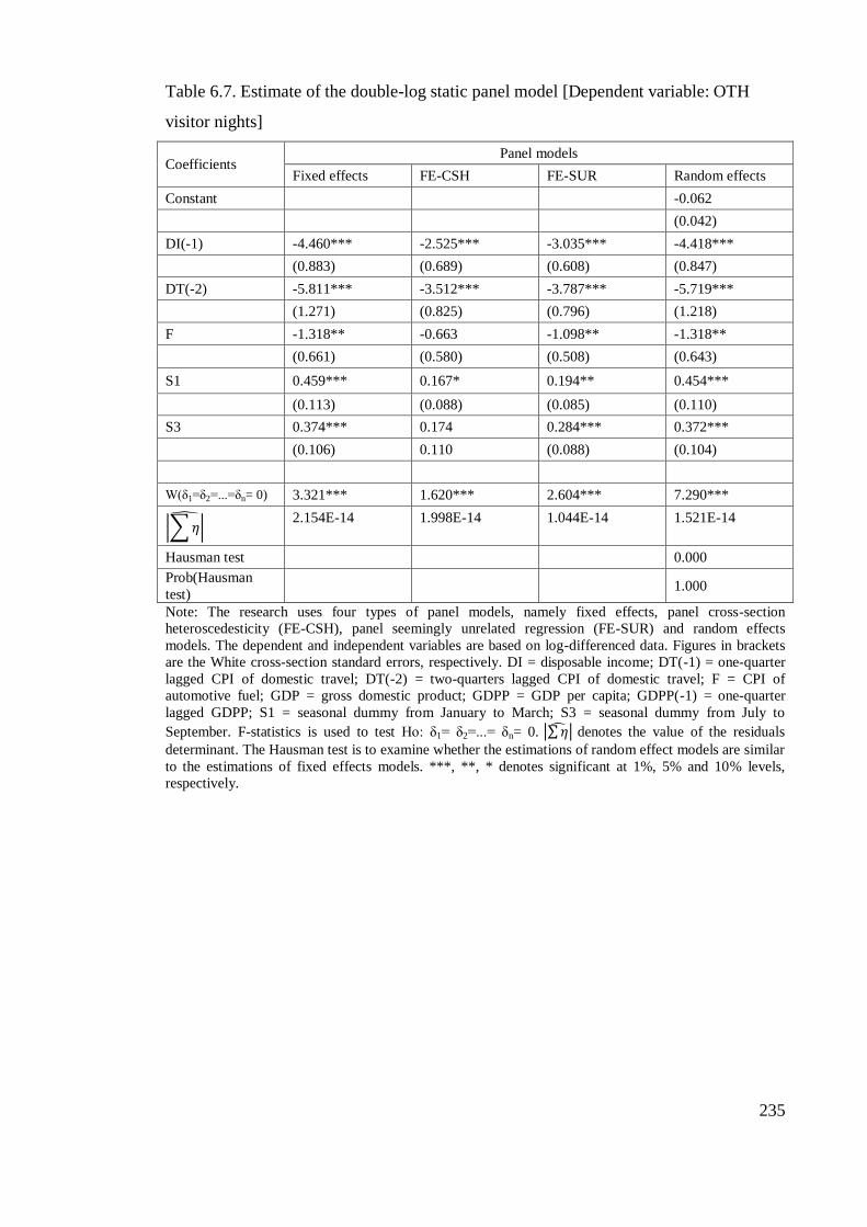
235
Table 6.7. Estimate of the double-log static panel model [Dependent variable: OTH
visitor nights]
Coefficients Panel models
Fixed effects FE-CSH FE-SUR Random effects
Constant
-0.062
(0.042)
DI(-1) -4.460*** -2.525*** -3.035*** -4.418***
(0.883) (0.689) (0.608) (0.847)
DT(-2) -5.811*** -3.512*** -3.787*** -5.719***
(1.271) (0.825) (0.796) (1.218)
F -1.318** -0.663 -1.098** -1.318**
(0.661) (0.580) (0.508) (0.643)
S1 0.459*** 0.167* 0.194** 0.454***
(0.113) (0.088) (0.085) (0.110)
S3 0.374*** 0.174 0.284*** 0.372***
(0.106) 0.110 (0.088) (0.104)
W(δ1=δ2=...=δn= 0) 3.321*** 1.620*** 2.604*** 7.290***
𝜂
2.154E-14
1.998E-14
1.044E-14
1.521E-14
Hausman test 0.000
Prob(Hausman
test) 1.000
Note: The research uses four types of panel models, namely fixed effects, panel cross-section
heteroscedesticity (FE-CSH), panel seemingly unrelated regression (FE-SUR) and random effects
models. The dependent and independent variables are based on log-differenced data. Figures in brackets
are the White cross-section standard errors, respectively. DI = disposable income; DT(-1) = one-quarter
lagged CPI of domestic travel; DT(-2) = two-quarters lagged CPI of domestic travel; F = CPI of
automotive fuel; GDP = gross domestic product; GDPP = GDP per capita; GDPP(-1) = one-quarter
lagged GDPP; S1 = seasonal dummy from January to March; S3 = seasonal dummy from July to
September. F-statistics is used to test Ho: δ1= δ2=...= δn= 0. 𝜂 denotes the value of the residuals
determinant. The Hausman test is to examine whether the estimations of random effect models are similar
to the estimations of fixed effects models. ***, **, * denotes significant at 1%, 5% and 10% levels,
respectively.

236
Table 6.8. Estimate of the double-log static panel model [Dependent variable: Interstate
visitor nights (NV)]
Coefficients Panel models
Fixed effects FE-CSH FE-SUR Random effects
Constant
-0.013
(0.033)
GDPP -6.971* -5.369* -6.704** -6.917*
(3.889) (2.527) (3.002) (3.856)
DT(-1) -2.128** -0.917 -1.403** -2.076**
(1.020) (0.644) (0.630) (1.036)
DT(-2) -4.131*** -2.767*** -2.620*** -4.090***
(0.472) (0.334) (0.300) (0.488)
Bali 0.249*** 0.222*** 0.220*** 0.248***
(0.054) (0.041) (0.064) (0.053)
S1 0.283*** 0.359*** 0.328*** 0.281***
(0.080) (0.049) (0.054) (0.080)
S3 0.073 0.111** 0.113*** 0.076
(0.058) (0.044) (0.041) (0.058)
W(δ1=δ2=...=δn= 0) 5.256*** 10.221*** 6.362*** 10.522***
𝜂
1.604E-14
8.826E-15
3.442E-15
2.942E-15
Hausman test
Prob(Hausman
test)
Note: The research uses four types of panel models, namely fixed effects, panel cross-section
heteroscedesticity (FE-CSH), panel seemingly unrelated regression (FE-SUR) and random effects
models. The dependent and independent variables are based on log-differenced data. Figures in brackets
are the White cross-section standard errors, respectively. Bali = dummy variable for bombing incidents in
Bali; DT(-1) = one-quarter lagged CPI of domestic travel; DT(-2) = two-quarters lagged CPI of domestic
travel; GDPP = GDP per capita; S1 = seasonal dummy from January to March; S3 = seasonal dummy
from July to September. F-statistics is used to test Ho: δ1= δ2=...= δn= 0. 𝜂 denotes the value of the
residuals determinant. The Hausman test is to examine whether the estimations of random effect models
are similar to the estimations of fixed effects models. ***, **, * denotes significant at 1%, 5% and 10%
levels, respectively.

237
Table 6.9. Estimate of the double-log static panel model [Dependent variable: Intrastate
visitor nights (NVI)]
Coefficients Panel models
Fixed effects FE-CSH FE-SUR Random effects
Constant
0.046
(0.032)
DT(-1) -1.262* -0.620 * -0.671** -1.260*
(0.708) (0.361) (0.310) (0.726)
DT(-2) -2.328*** -0.772 *** -0.676 ** -2.324***
(0.618) (0.243) (0.306) (0.622)
Bali 0.124*** 0.106*** 0.083** 0.124***
(0.033) (0.034) (0.033) (0.033)
S1 0.276*** 0.177*** 0.191*** 0.276***
(0.056) (0.028) (0.024) (0.056)
S2 -0.131* -0.290*** -0.254*** -0.132*
(0.069) (0.036) (0.038) (0.068)
S3 -0.224*** -0.228*** -0.210*** -0.224***
(0.049) (0.026) (0.026) (0.049)
W(δ1=δ2=...=δn= 0) 9.844*** 29.063*** 21.418*** 20.168***
𝜂
4.566E-15
1.546E-14
1.818E-15
4.330E-15
Hausman test 0.000
Prob(Hausman
test) 1.000
Note: The research uses four types of panel models, namely fixed effects, panel cross-section
heteroscedesticity (FE-CSH), panel seemingly unrelated regression (FE-SUR) and random effects
models. The dependent and independent variables are based on log-differenced data. Figures in brackets
are the White cross-section standard errors, respectively. Bali = dummy variable for bombing incidents in
Bali; DT(-1) = one-quarter lagged CPI of domestic travel; DT(-2) = two-quarters lagged CPI of domestic
travel; S1 = seasonal dummy from January to March; S2 = seasonal dummy from April to June; S3 =
seasonal dummy from July to September. F-statistics is used to test Ho: δ1= δ2=...= δn= 0. 𝜂 denotes
the value of the residuals determinant. The Hausman test is to examine whether the estimations of random
effect models are similar to the estimations of fixed effects models. ***, **, * denotes significant at 1%,
5% and 10% levels, respectively.

238
Table 6.10. Estimate of the double-log static panel model [Dependent variable: Number
of interstate visitors (OV)]
Coefficients Panel models
Fixed effects FE-CSH FE-SUR Random effects
Constant
-0.124***
(0.041)
GDPP -5.764** -4.100*** -3.417** -5.771**
(2.509) (1.414) (1.466) (2.470)
DT(-2) -3.914*** -1.114*** -1.373*** -3.881***
(0.651) (0.381) (0.343) (0.644)
Bali 0.160*** 0.105*** 0.066** 0.159***
(0.041) (0.028) (0.029) (0.041)
S1 0.237*** 0.098*** 0.111*** 0.235***
(0.068) (0.033) (0.029) (0.068)
S2 0.349*** 0.078* 0.102** 0.347***
(0.083) (0.046) (0.044) (0.081)
S3 0.152*** 0.060** 0.101*** 0.152***
(0.049) (0.029) (0.028) (0.048)
W(δ1=δ2=...=δn= 0) 4.738*** 1.741* 1.175 9.512***
𝜂
1.787E-14
2.220E-15
3.775E-15
2.076E-14
Hausman test 0.000
Prob(Hausman
test) 1.000
Note: The research uses four types of panel models, namely fixed effects, panel cross-section
heteroscedesticity (FE-CSH), panel seemingly unrelated regression (FE-SUR) and random effects
models. The dependent and independent variables are based on log-differenced data. Figures in brackets
are the White cross-section standard errors, respectively. Bali = dummy variable for bombing incidents in
Bali; DT(-2) = two-quarters lagged CPI of domestic travel; GDPP = GDP per capita; S1 = seasonal
dummy from January to March; S2 = seasonal dummy from April to June; S3 = seasonal dummy from
July to September. F-statistics is used to test Ho: δ1= δ2=...= δn= 0. 𝜂 denotes the value of the residuals
determinant. The Hausman test is to examine whether the estimations of random effect models are similar
to the estimations of fixed effects models. ***, **, * denotes significant at 1%, 5% and 10% levels,
respectively.

239
Table 6.11. Estimate of the double-log static panel model [Dependent variable: Number
of intrastate visitors (OVI)]
Coefficients Panel models
Fixed effects FE-CSH FE-SUR Random effects
Constant
0.034
(0.025)
DT(-1) -0.720* -0.490 -0.734** -0.716
(0.424) (0.315) (0.303) (0.436)
DT(-2) -1.748*** -0.587*** -0.605** -1.739***
(0.374) (0.217) (0.246) (0.369)
Bali 0.087*** 0.068*** 0.068*** 0.087***
(0.025) (0.023) (0.023) (0.025)
S1 0.110** 0.044* 0.062** 0.110**
(0.045) (0.026) (0.026) (0.044)
S2 -0.012 -0.103*** -0.110*** -0.013
(0.047) (0.031) (0.031) (0.046)
S3 -0.169*** -0.169*** -0.180*** -0.169***
(0.034) (0.028) (0.028) (0.034)
W(δ1=δ2=...=δn= 0) 5.846*** 10.133*** 6.386*** 11.932***
𝜂
1.998E-15
5.163E-15
2.776E-15
6.41E-15
Hausman test 0.000
Prob(Hausman
test) 1.000
Note: The research uses four types of panel models, namely fixed effects, panel cross-section
heteroscedesticity (FE-CSH), panel seemingly unrelated regression (FE-SUR) and random effects
models. The dependent and independent variables are based on log-differenced data. Figures in brackets
are the White cross-section standard errors, respectively. Bali = dummy variable for bombing incidents in
Bali; DT(-1) = one-quarter lagged CPI of domestic travel; DT(-2) = two-quarters lagged CPI of domestic
travel; S1 = seasonal dummy from January to March; S2 = seasonal dummy from April to June; S3 =
seasonal dummy from July to September. F-statistics is used to test Ho: δ1= δ2=...= δn= 0. 𝜂 denotes
the value of the residuals determinant. The Hausman test is to examine whether the estimations of random
effect models are similar to the estimations of fixed effects models. ***, **, * denotes significant at 1%,
5% and 10% levels, respectively.

240
The residuals determinants are reported in the tables in order to determine the best
statistical representation of each category of domestic tourists. Accordingly, the best
model is justified by the criterion of the minimum value of the determinants. Based on
the results, the best static panel data models for holiday and OTH tourism demand are
FE-SUR, whilst FE-CSH is the best model for business, VFR and intrastate overnight
tourism demand. As for interstate overnight tourism demand, the fixed effects model
has the lowest value of residuals determinants.
Even though the static panel data models have generated convincing estimates, we
cannot be sure that the models are completely free of specification errors. As it is widely
known in tourism literature that tourists tend to have habit persistency, omitting such
information could lead to serious misspecification. Hence, in the following section,
dynamic panel data models are employed by adding lagged dependent variables to take
account of tourists‟ habit persistency.
6.5 Panel data dynamic models
For the purposes of accommodating lagged dependent variables into a fixed effects
model, it can be done by transforming the regressions into a dynamic panel data model.
To illustrate the point, the panel data with serial correlation model is developed as
follows:
,'
jtjtjt vy (6.7)
jttjjt 1,
where 1 and jt are independent and identically distributed.
Equation (6.7) can be re-written as shown below.
jtjtjtjtjt vvyy )( 11 (6.8)
Or
jtjtjtjt vyy
*
1 , where *
jtv = 1 jtjt vv

241
All coefficients in equation (6.8) have become more consistent and efficient compared
to the estimates in equation (6.2). Nevertheless, estimating equation (6.8) using least
squares is problematic because the lagged dependent variable is correlated with the
disturbance, even if jt is not serially correlated. Hence, to overcome this issue, the
most appropriate estimation method is to employ the instrumental variables techniques.
Nevertheless, the necessary condition is that the instrumental variables (i.e. yjt-2) must
display strict exogeneity, E( jt /yjt-2) = 0 for all t.
For this thesis, three types of instrumental variables models are considered, namely the
Two-Stage Least Squares (2SLS), weighted 2SLS (W2SLS) and the Three-Stage Least
Squares (3SLS). Note that, the W2SLS model follows the Keane and Runkle (1992)
procedure. It takes accounts of heteroscedasticity in the residuals when some of the
right-hand side variables are correlated with the error terms. The benefit of the model is
that it can gain in efficiency in performing the procedure on a first-differenced model
[Baltagi (2008)]. Similarly, the 3SLS model takes account of both heteroscedasticity
and contemporary correlation in the residuals. To put it differently, the 3SLS model is
the two-stage least squares version of the SUR method [Ledesma-Rodriguez et al.
(2001)].
This thesis includes a unit root test for dynamic panels, which is developed by Harris
and Tzavalis (1999). They introduced asymptotic unit root tests where the residuals
follow an AR(1) and the time dimension is fixed. The test derived is based on the
normalised least squares estimators of the autoregressive coefficient and allow for fixed
effects and individual deterministic trends [Harris and Tzavalis (1999, pg.202)]. The
authors considered three data generating processes (DGP). One of them is written as
follows:
𝑙𝑜𝑔 𝑦𝑖𝑡 = 𝜔𝑖 + 𝜌 𝑙𝑜𝑔 𝑦𝑖,𝑡−1 + 𝑢𝑖𝑡 (6.9)
where 𝑦𝑖𝑡 = some relevant variable, ω and ρ are parameters, and 𝑢𝑖𝑡 ≈ 𝑁𝑖𝑖𝑑 0, 𝜎𝑢2 .
The null hypothesis is the existence of a unit root in equation 6.9 (i.e. ρ = 1) and the

242
alternative hypothesis is that the AR(1) process is stationary, i.e. 𝜌 < 1. The model is
a unit root process with heterogeneous drift parameters under the null hypothesis, and a
stationary process with heterogeneous intercepts under the alternative hypothesis. The
normalised distribution of the statistic is:
𝑁(𝜌 − 1 − 𝐵)𝐿 𝑁(0, 𝐶)
where 𝐵 = −3 𝑇 + 1 −1,
𝐶 = 3 17𝑇2 − 20𝑇 + 17 5 𝑇 − 1 (𝑇 + 1)3 −1
Tables 6.12 – 6.19 present the empirical results for the dynamic panels. Compared to
the findings in previous subsection, the coefficients for GDPP(-1) and DT(-1) become
insignificant for holiday and interstate tourism demand, respectively. Moreover, the
GDPP estimate is found to be statistically significant for interstate visitor night data.
However, for the coefficient for GDPP(-1), this variable is found to be statistically
insignificant for holiday visitor night case and therefore, it is omitted from this study.
For the rest of the variables, the elasticities vary slightly from the results that appear in
Tables 6.4 – 6.11.
The coefficients for lagged dependent variables in all cases are found to be statistically
significant at the 1% level. Nevertheless, the coefficient sign for Yj,t-1 is negative for all
cases, implying that the lagged dependent variables have negative effects on Australian
domestic tourism demand. It may be that Australian domestic visitors make periodic
interstate or intrastate trips for holidaying, business or visiting relatives and friends. On
the face of it, this suggests a negative reaction to previous demand. We suspect that
there is probably a strong periodic demand element in this. If they have travelled in the
recent past, they are unlikely to travel again in the near future. This is supported by the
significance of lagged seasonal variables in most cases. Furthermore, one issue with our
data is that it is drawn from a sample, undertaken at periodic intervals, which means our
observations do not reflect the behaviour of the same individual tourists.
In regard to the robustness of the models, the F-statistics reject the null hypothesis of
δ1= δ2=...= δn=0 (i.e. all coefficients are jointly zero) at a 1% significance level,

243
indicating that all explanatory variables are important and independent in explaining
domestic tourism demand. Moreover, based on the Harris and Tzavalis test of unit roots
in dynamic panels, the student t-test rejects the null hypothesis of ρ=1 in most cases,
concluding that Yj,t-1 follows a stationary stochastic process, that is AR(1). However,
the test fails to reject the null hypothesis in the 2SLS and W2SLS estimations of holiday
visitor night, and the 2SLS estimations of interstate tourism demand data.
Furthermore, some of the results in the IPS test are not consistent with the Harris and
Tzavalis test. Referring to Tables 6.2 and 6.3 above, the IPS test suggests that all first-
differenced data are stationary. However, the Harris and Tzavalis (HT) test found the
existence of unit root for HOL, NV, NVI, OV and OVI cases. A possible reason is that
the IPS test might have less power than the HT test because the former examines unit
root test based on individual time series case, whereas the latter investigates asymptotic
unit root for first-order autoregressive panel data models. Furthermore, according to
Harris and Tzavalis (1999), Monte Carlo evidence suggests that the HT test has
substantially more power than the unit root tests for the single time series case.
Overall, Tables 6.12 – 6.19 suggest that the 3SLS estimation obtains better results for
holiday, business, VFR visitor nights as well as the intrastate visitor data. Furthermore,
the best estimation results for OTH and intrastate visitor night data are the 2SLS
estimation, whilst the best model used for modelling interstate tourism demand is the
W2SLS. The conclusion is made based on the criterion of the minimum value of the
residual determinants and stationary stochastic process of AR(1).
6.6 Investigating other related factors affecting Australian domestic
tourism demand
In this section, other related factors, namely household debt, consumers‟ perceptions
about the future economy and working hours, are investigated to examine whether they
have an influence on Australian domestic tourism demand. The main intention is to

244
Table 6.12. Estimate of the double-log panel model with dynamic [Dependent variable:
Holiday visitor nights (HOL)]
Coefficients Dynamic panel models
2SLS W2SLS 3SLS
DT(-1) -2.048** -0.674 -1.261**
(0.988) (0.435) (0.629)
DT(-2) -7.265*** -2.198*** -3.535***
(1.101) (0.436) (0.530)
Bali 0.260*** 0.105*** 0.151***
(0.080) (0.030) (0.049)
S1 0.711*** 0.510*** 0.527***
(0.119) (0.045) (0.053)
S2 0.224** -0.204*** -0.028
(0.095) (0.036) (0.062)
Yj,t-1 -0.207* -0.226* -0.413***
(0.121) (0.118) (0.048)
W(δ1=δ2=...=δn= 0) 8.551*** 20.514*** 13.005***
𝜂
1.532E-14
1.704E-14
4.285E-14
t(ρ=1) -9.955 -10.364 -29.734
Note: The research uses three types of dynamic panel models, namely two-stage least squares (2SLS),
weighted two-stage least squares (W2SLS), three-stage least squares (3SLS) models. A dynamic model
can be written as: jtjtjtjt vyy
*
1 , where *
jtv = 1 jtjt vv ,
jty = demand for
domestic tourism in State j, v = a vector of independent variables, t = time subscript, = a coefficient
matrix, and jt = errors from different cross-section units. The 2SLS model assumes no
heteroscedasticity and contemporary correlation in the residuals. The W2SLS model only takes account
of heteroscedasticity, whereas the 3SLS model takes account of both heteroscedasticity and contemporary
correlation. The dependent and independent variables are based on log-differenced data. Figures in
brackets are the White cross-section standard errors, respectively. Bali = dummy variable for bombing
incidents in Bali; DT(-1) = one-quarter lagged CPI of domestic travel; DT(-2) = two-quarters lagged CPI
of domestic travel; Yj,t-1 = lagged dependent variables; S1 = seasonal dummy from January to March; S2
= seasonal dummy from April to June. Estimates are obtained using instrument to Yj,t-2. ***, **, *
denotes significant at 1%, 5% and 10% levels, respectively. F-statistics is used to test the joint
significance of the parameters, i.e. Ho: δ1= δ2=...= δn= 0. 𝜂 denotes the value of the residuals
determinant. t(ρ=1) is the t-values for testing ρ=1 to test the existence of unit roots in the dynamic panel
model [See Harris and Tzavalis (1999) for more details]. The normalised coefficients for the Harris and
Tzavalis test of ρ=1 are -19.534, -18.996, and -13.795.

245
Table 6.13. Estimate of the double-log panel model with dynamic [Dependent variable:
Business visitor nights (BUS)]
Coefficients Dynamic panel models
2SLS W2SLS 3SLS
GDP 1.847** 1.473** 1.536**
(0.738) (0.723) (0.679)
GDPP(-1) 7.596*** 6.597** 5.885**
(2.709) (2.888) (2.611)
DT(-1) -1.209** -1.160** -1.394***
(0.529) (0.525) (0.510)
Yj,t-1 -0.554*** -0.539*** -0.544***
(0.061) (0.053) (0.048)
W(δ1=δ2=...=δn= 0) 13.123*** 11.503*** 11.260***
𝜂
0
9.992E-16
0
t(ρ=1) -25.532 -29.263 -31.983
Note: The research uses three types of dynamic panel models, namely two-stage least squares (2SLS),
weighted two-stage least squares (W2SLS), three-stage least squares (3SLS) models. A dynamic model
can be written as: jtjtjtjt vyy
*
1 , where *
jtv = 1 jtjt vv ,
jty = demand for
domestic tourism in State j, v = a vector of independent variables, t = time subscript, = a coefficient
matrix, and jt = errors from different cross-section units. The 2SLS model assumes no
heteroscedasticity and contemporary correlation in the residuals. The W2SLS model only takes account
of heteroscedasticity, whereas the 3SLS model takes account of both heteroscedasticity and contemporary
correlation. The dependent and independent variables are based on log-differenced data. Figures in
brackets are the White cross-section standard errors, respectively. DT(-1) = one-quarter lagged CPI of
domestic travel; DT(-2) = two-quarters lagged CPI of domestic travel; GDPP = GDP per capita; GDPP(-
1) = one-quarter lagged GDPP; Yj,t-1 = lagged dependent variables. Estimates are obtained using
instrument to Yj,t-2. ***, **, * denotes significant at 1%, 5% and 10% levels, respectively. F-statistics is
used to test the joint significance of the parameters, i.e. Ho: δ1= δ2=...= δn= 0. 𝜂 denotes the value of
the residuals determinant. t(ρ=1) is the t-values for testing ρ=1 to test the existence of unit roots in the
dynamic panel model [See Harris and Tzavalis (1999) for more details]. The normalised coefficients for
the Harris and Tzavalis test of ρ=1 are -9.884, -10.295, and -10.160.

246
Table 6.14. Estimate of the double-log panel model with dynamic [Dependent variable:
VFR visitor nights]
Coefficients Dynamic panel models
2SLS W2SLS 3SLS
DI -2.699*** -1.492*** -1.630***
(0.889) (0.450) (0.616)
DT(-2) -5.172*** -2.074*** -2.541***
(0.880) (0.412) (0.525)
Bali 0.212* 0.124* 0.128
(0.110) (0.069) (0.081)
S1 0.032 -0.066 -0.011
(0.164) (0.073) (0.092)
S2 0.101 -0.191*** -0.120**
(0.092) (0.048) (0.055)
S3 -0.068 -0.201*** -0.134**
(0.118) (0.048) (0.065)
Yj,t-1 -0.545*** -0.426*** -0.535***
(0.084) (0.074) (0.054)
W(δ1=δ2=...=δn= 0) 15.0*** 16.693*** 13.486***
𝜂
1.688E-14
4.380E-15
1.310E-14
t(ρ=1) -18.385 -19.186 -28.347
Note: The research uses three types of dynamic panel models, namely two-stage least squares (2SLS),
weighted two-stage least squares (W2SLS), three-stage least squares (3SLS) models. A dynamic model
can be written as: jtjtjtjt vyy
*
1 , where *
jtv = 1 jtjt vv ,
jty = demand for
domestic tourism in State j, v = a vector of independent variables, t = time subscript, = a coefficient
matrix, and jt = errors from different cross-section units. The 2SLS model assumes no
heteroscedasticity and contemporary correlation in the residuals. The W2SLS model only takes account
of heteroscedasticity, whereas the 3SLS model takes account of both heteroscedasticity and contemporary
correlation. The dependent and independent variables are based on log-differenced data. Figures in
brackets are the White cross-section standard errors, respectively. Bali = dummy variable for bombing
incidents in Bali; DI = disposable income; DT(-2) = two-quarters lagged CPI of domestic travel; F = CPI
of automotive fuel; GDP = gross domestic product; GDPP = GDP per capita; GDPP(-1) = one-quarter
lagged GDPP; Yj,t-1 = lagged dependent variables; S1 = seasonal dummy from January to March; S2 =
seasonal dummy from April to June; S3 = seasonal dummy from July to September. Estimates are
obtained using instrument to Yj,t-2. ***, **, * denotes significant at 1%, 5% and 10% levels, respectively.
F-statistics is used to test the joint significance of the parameters, i.e. Ho: δ1= δ2=...= δn= 0. 𝜂 denotes
the value of the residuals determinant. t(ρ=1) is the t-values for testing ρ=1 to test the existence of unit
roots in the dynamic panel model [See Harris and Tzavalis (1999) for more details]. The normalised
coefficients for the Harris and Tzavalis test of ρ=1 are -10.350, -12.753, and -10.411.

247
Table 6.15. Estimate of the double-log panel model with dynamic [Dependent variable:
OTH visitor nights]
Coefficients Dynamic panel models
2SLS W2SLS 3SLS
DI(-1) -4.347*** -1.820** -3.0***
(0.892) (0.755) (0.709)
DT(-2) -6.089*** -2.846*** -3.827***
(1.259) (0.793) (0.826)
F -0.780 -0.436 -0.613
(0.571) (0.457) (0.412)
S1 0.478*** 0.095 0.213*
(0.151) (0.118) (0.122)
S3 0.370** 0.099 0.267**
(0.155) (0.139) (0.114)
Yj,t-1 -0.380*** -0.402*** -0.415***
(0.073) (0.045) (0.043)
W(δ1=δ2=...=δn= 0) 6.508*** 5.355*** 6.145***
𝜂
1.743E-14
1.776E-15
4.885E-15
t(ρ=1) -18.976 -31.344 -32.637
Note: The research uses three types of dynamic panel models, namely two-stage least squares (2SLS),
weighted two-stage least squares (W2SLS), three-stage least squares (3SLS) models. A dynamic model
can be written as: jtjtjtjt vyy
*
1 , where *
jtv = 1 jtjt vv ,
jty = demand for
domestic tourism in State j, v = a vector of independent variables, t = time subscript, = a coefficient
matrix, and jt = errors from different cross-section units. The 2SLS model assumes no
heteroscedasticity and contemporary correlation in the residuals. The W2SLS model only takes account
of heteroscedasticity, whereas the 3SLS model takes account of both heteroscedasticity and contemporary
correlation. The dependent and independent variables are based on log-differenced data. Figures in
brackets are the White cross-section standard errors, respectively. Bali = dummy variable for bombing
incidents in Bali; DI = disposable income; DT(-2) = two-quarters lagged CPI of domestic travel; F = CPI
of automotive fuel; Yj,t-1 = lagged dependent variables, S3 = seasonal dummy from July to September;
and S4 = seasonal dummy from October to December. Estimates are obtained using instrument to Yj,t-2.
***, **, * denotes significant at 1%, 5% and 10% levels, respectively. F-statistics is used to test the joint
significance of the parameters, i.e. Ho: δ1= δ2=...= δn= 0. 𝜂 denotes the value of the residuals
determinant. t(ρ=1) is the t-values for testing ρ=1 to test the existence of unit roots in the dynamic panel
model [See Harris and Tzavalis (1999) for more details]. The normalised coefficients for the Harris and
Tzavalis test of ρ=1 are -14.736, -14.105, and -13.739.

248
Table 6.16. Estimate of the double-log panel model with dynamic [Dependent variable:
Interstate visitor nights (NV)]
Coefficients Dynamic panel models
2SLS W2SLS 3SLS
GDPP -3.457 -4.098* -4.341
(3.444) (2.282) (2.869)
DT(-1) -1.586** -0.033 -0.936*
(0.804) (0.552) (0.514)
DT(-2) -4.335*** -2.763*** -2.762***
(0.664) (0.389) (0.362)
Bali 0.244*** 0.183*** 0.187**
(0.084) (0.063) (0.075)
S1 0.302*** 0.335*** 0.325***
(0.092) (0.056) (0.066)
S3 0.101 0.162*** 0.149**
(0.075) (0.058) (0.071)
Yj,t-1 -0.262** -0.327*** -0.461***
(0.102) (0.074) (0.046)
W(δ1=δ2=...=δn= 0) 6.109*** 11.179*** 10.690***
𝜂
2.193E-14
2.670E-14
3.231E-14
t(ρ=1) -12.429 -17.863 -31.440
Note: The research uses three types of dynamic panel models, namely two-stage least squares (2SLS),
weighted two-stage least squares (W2SLS), three-stage least squares (3SLS) models. A dynamic model
can be written as: jtjtjtjt vyy
*
1 , where *
jtv = 1 jtjt vv ,
jty = demand for
domestic tourism in State j, v = a vector of independent variables, t = time subscript, = a coefficient
matrix, and jt = errors from different cross-section units. The 2SLS model assumes no
heteroscedasticity and contemporary correlation in the residuals. The W2SLS model only takes account
of heteroscedasticity, whereas the 3SLS model takes account of both heteroscedasticity and contemporary
correlation. The dependent and independent variables are based on log-differenced data. Figures in
brackets are the White cross-section standard errors, respectively. Bali = dummy variable for bombing
incidents in Bali; DT(-1) = one-quarter lagged CPI of domestic travel; DT(-2) = two-quarters lagged CPI
of domestic travel; Yj,t-1 = lagged dependent variables; S1 = seasonal dummy from January to March; S3
= seasonal dummy from July to September; and S4 = seasonal dummy from October to December.
Estimates are obtained using instrument to Yj,t-2. ***, **, * denotes significant at 1%, 5% and 10% levels,
respectively. F-statistics is used to test the joint significance of the parameters, i.e. Ho: δ1= δ2=...= δn= 0.
𝜂 denotes the value of the residuals determinant. t(ρ=1) is the t-values for testing ρ=1 to test the
existence of unit roots in the dynamic panel model [See Harris and Tzavalis (1999) for more details]. The
normalised coefficients for the Harris and Tzavalis test of ρ=1 are -18.011, -16.192, and -12.462.

249
Table 6.17. Estimate of the double-log panel model with dynamic [Dependent variable:
Intrastate visitor nights (NVI)]
Coefficients Dynamic panel models
2SLS W2SLS 3SLS
DT(-2) -2.344*** -0.856*** -0.682**
(0.548) (0.307) (0.311)
Bali 0.10*** 0.092** 0.039
(0.033) (0.046) (0.033)
S1 0.266*** 0.178*** 0.213***
(0.064) (0.034) (0.032)
S2 -0.120** -0.286*** -0.244***
(0.060) (0.040) (0.035)
S3 -0.170*** -0.218*** -0.151***
(0.047) (0.025) (0.029)
Yj,t-1 -0.386*** -0.299*** -0.492***
(0.081) (0.083) (0.055)
W(δ1=δ2=...=δn= 0) 14.358*** 28.166*** 25.203***
𝜂
6.967E-15
8.535E-16
8.965E-15
t(ρ=1) -17.104 -15.603 -26.989
Note: The research uses three types of dynamic panel models, namely two-stage least squares (2SLS),
weighted two-stage least squares (W2SLS), three-stage least squares (3SLS) models. A dynamic model
can be written as: jtjtjtjt vyy
*
1 , where *
jtv = 1 jtjt vv ,
jty = demand for
domestic tourism in State j, v = a vector of independent variables, t = time subscript, = a coefficient
matrix, and jt = errors from different cross-section units. The 2SLS model assumes no
heteroscedasticity and contemporary correlation in the residuals. The W2SLS model only takes account
of heteroscedasticity, whereas the 3SLS model takes account of both heteroscedasticity and contemporary
correlation. The dependent and independent variables are based on log-differenced data. Figures in
brackets are the White cross-section standard errors, respectively. Bali = dummy variable for bombing
incidents in Bali; DT(-2) = two-quarters lagged CPI of domestic travel; Yj,t-1 = lagged dependent
variables; S1 = seasonal dummy from January to March; S2 = seasonal dummy from April to June; S3 =
seasonal dummy from July to September; and S4 = seasonal dummy from October to December.
Estimates are obtained using instrument to Yj,t-2. ***, **, * denotes significant at 1%, 5% and 10% levels,
respectively. F-statistics is used to test the joint significance of the parameters, i.e. Ho: δ1= δ2=...= δn= 0.
𝜂 denotes the value of the residuals determinant. t(ρ=1) is the t-values for testing ρ=1 to test the
existence of unit roots in the dynamic panel model [See Harris and Tzavalis (1999) for more details]. The
normalised coefficients for the Harris and Tzavalis test of ρ=1 are -14.561, -16.977, and -11.599. The
coefficient for DT(-1) are found to be statistically insignificant and therefore, this variable is omitted from
the study.

250
Table 6.18. Estimate of the double-log panel model with dynamic [Dependent variable:
Number of interstate visitors (OV)]
Coefficients Dynamic panel models
2SLS W2SLS 3SLS
GDPP -6.001** -3.782** -3.193**
(2.718) (1.486) (1.278)
DT(-2) -4.387*** -1.477*** -1.875***
(0.626) (0.332) (0.305)
Bali 0.168*** 0.102*** 0.109***
(0.049) (0.032) (0.039)
S1 0.284*** 0.129*** 0.166***
(0.083) (0.039) (0.036)
S2 0.380*** 0.093** 0.145***
(0.077) (0.044) (0.041)
S3 0.166** 0.066* 0.113***
(0.069) (0.035) (0.041)
Yj,t-1 -0.286*** -0.331*** -0.444***
(0.101) (0.073) (0.052)
W(δ1=δ2=...=δn= 0) 5.829*** 3.997*** 5.495***
𝜂
1.33227E-15
1.155E-14
6.162E-15
t(ρ=1) -12.684 -18.310 -27.662
Note: The research uses three types of dynamic panel models, namely two-stage least squares (2SLS),
weighted two-stage least squares (W2SLS), three-stage least squares (3SLS) models. A dynamic model
can be written as: jtjtjtjt vyy
*
1 , where *
jtv = 1 jtjt vv ,
jty = demand for
domestic tourism in State j, v = a vector of independent variables, t = time subscript, = a coefficient
matrix, and jt = errors from different cross-section units. The 2SLS model assumes no
heteroscedasticity and contemporary correlation in the residuals. The W2SLS model only takes account
of heteroscedasticity, whereas the 3SLS model takes account of both heteroscedasticity and contemporary
correlation. The dependent and independent variables are based on log-differenced data. Figures in
brackets are the White cross-section standard errors, respectively. Bali = dummy variable for bombing
incidents in Bali; DT(-2) = two-quarters lagged CPI of domestic travel; GDPP = GDP per capita; GDPP(-
1) = one-quarter lagged GDPP; Yj,t-1 = lagged dependent variables; S1 = seasonal dummy from January to
March; S2 = seasonal dummy from April to June; S3 = seasonal dummy from July to September; and S4
= seasonal dummy from October to December. Estimates are obtained using instrument to Yj,t-2. ***, **, *
denotes significant at 1%, 5% and 10% levels, respectively. F-statistics is used to test the joint
significance of the parameters, i.e. Ho: δ1= δ2=...= δn= 0. 𝜂 denotes the value of the residuals
determinant. t(ρ=1) is the t-values for testing ρ=1 to test the existence of unit roots in the dynamic panel
model [See Harris and Tzavalis (1999) for more details]. The normalised coefficients for the Harris and
Tzavalis test of ρ=1 are -17.352, -16.081, and -12.941.

251
Table 6.19. Estimate of the double-log panel model with dynamic [Dependent variable:
Number of intrastate visitors (OVI)]
Coefficients Dynamic panel models
2SLS W2SLS 3SLS
DT(-2) -1.833*** -0.763*** -0.752***
(0.353) (0.245) (0.219)
Bali 0.074** 0.065* 0.064*
(0.035) (0.034) (0.034)
S1 0.110** 0.051* 0.071**
(0.051) (0.031) (0.033)
S2 -0.008 -0.104*** -0.106***
(0.042) (0.034) (0.031)
S3 -0.137*** -0.162*** -0.162***
(0.033) (0.026) (0.028)
Yj,t-1 -0.313*** -0.234*** -0.340***
(0.085) (0.079) (0.058)
W(δ1=δ2=...=δn= 0) 8.194*** 11.497*** 9.208***
𝜂
2.276E-15
3.553E-15
4.413E-15
t(ρ=1) -15.504 -15.650 -23.163
Note: The research uses three types of dynamic panel models, namely two-stage least squares (2SLS),
weighted two-stage least squares (W2SLS), three-stage least squares (3SLS) models. A dynamic model
can be written as: jtjtjtjt vyy
*
1 , where *
jtv = 1 jtjt vv ,
jty = demand for
domestic tourism in State j, v = a vector of independent variables, t = time subscript, = a coefficient
matrix, and jt = errors from different cross-section units. The 2SLS model assumes no
heteroscedasticity and contemporary correlation in the residuals. The W2SLS model only takes account
of heteroscedasticity, whereas the 3SLS model takes account of both heteroscedasticity and contemporary
correlation. The dependent and independent variables are based on log-differenced data. Figures in
brackets are the White cross-section standard errors, respectively. Bali = dummy variable for bombing
incidents in Bali; DT(-2) = two-quarters lagged CPI of domestic travel; Yj,t-1 = lagged dependent
variables; S1 = seasonal dummy from January to March; S2 = seasonal dummy from April to June; S3 =
seasonal dummy from July to September; and S4 = seasonal dummy from October to December.
Estimates are obtained using instrument to Yj,t-2. ***, **, * denotes significant at 1%, 5% and 10% levels,
respectively. F-statistics is used to test the joint significance of the parameters, i.e. Ho: δ1= δ2=...= δn= 0.
𝜂 denotes the value of the residuals determinant. t(ρ=1) is the t-values for testing ρ=1 to test the
existence of unit roots in the dynamic panel model [See Harris and Tzavalis (1999) for more details]. The
normalised coefficients for the Harris and Tzavalis test of ρ=1 are -16.579, -18.780, and -15.849. The
coefficient for DT(-1) are found to be statistically insignificant and therefore, this variable is omitted from
the study.

252
evaluate how changes in other household expenditure, perceptions of economic outlook
and working life could affect Australians‟ preferences to do travelling.
This current research investigates the existence of the relationships between domestic
tourism demand and the above-mentioned indicators. With respect to this, a model of
domestic tourism demand is constructed as follows:
),,,,,( jtjtjtjtjtjtjt WORDEBTConExpDUMTPYfTD
where Y = domestic household income, TP = tourism prices, DUM = dummy variable
for one-off events (such as Bali bombings in 2005 and Sydney Olympic Games in 2000)
and seasonality, ConExp = consumers‟ expectations of the future economy, WOR =
working hours, and DEBT = household debt. The model is developed for three
purposes. First, we can estimate the income and tourism price elasticities, and determine
whether one-off events and seasonality have impacts on the demand. Second, the model
can be used to examine whether the consumers‟ perceptions, household debt and
number of worked hours in paid jobs influence Australian domestic tourism demand.
Lastly, it is of interest to assess whether these three variables should be included in or
excluded out from equation 6.8.
The additional four proxy variables used in this research are: (1) the consumer
sentiment index (CSI) to evaluate the impacts of consumers‟ perceptions of the future
economy on HOL and VFR tourism demand, (2) the business confidence index (BCI)
for business tourism demand analysis, (3) the ratio of interest repayment-to-disposable
income, and (4) the average actual worked hours in Australia. In this study, first
differenced data is employed and is based on a quarterly basis from 1999 to 2007. Table
6.20 presents an in-depth explanation of these additional variables used.

253
Table 6.20. List of additional variable used
Variable Notation Proxy for: Source Definition and the rational
explanation of using this proxy
variable
Average actual
worked hours
WOR Working
hours
ABS and
RBA
Definition: It calculates the average
hours worked in paid jobs in
Australia.
It is assumed that when the number
of actual working hours increases,
there is a tendency that Australian
households will forego domestic
travel. Therefore, the correlation
between the WOR and domestic
tourism demand is expected to be
negative.
Business
confidence index
BCI Consumers‟
perceptions of
future
economic
outlook
RBA Definition: The index measures
respondents‟ anticipations of
business conditions in their industry
for the upcoming quarter.
It is employed in this research as a
proxy for business travellers‟
perceptions of future economy. If
they perceive a positive growth in
their business, there is a possibility
that they will travel more frequently
for business purposes. Thus, the
expected sign for the variable is
positive.
Consumer
sentiment index
CSI Consumers‟
perceptions on
future
economic
outlook
MI/RBA Definition: It reflects the Australians'
views on current and prospective
household financial situation,
economic outlook and purchasing
power.
The relationships between the CSI
and Australian domestic tourism
demand are expected to be positive.
If Australian households are
optimistic about the future economy,
they will increase their current
spending and vice-versa.
Interest
repayments-to-
disposable
income ratio
DEBT Household
debt
RBA Definition: It indicates how much
disposable income has been used for
interest payments on housing and
other personal debt.
Based on the literature above, the
expected sign for this variable is
undetermined. On one hand, the sign
can be negative because the share of
domestic travel expenditure is
expected to decline if household debt
increases. On the other hand, the sign
can be positive as the growth rate of

254
Variable Notation Proxy for: Source Definition and the rational
explanation of using this proxy
variable
borrowing would encourage more
Australians to travel.
*TRA stands for Tourism Research Australia; ABS stands for the Australian Bureau of Statistics; RBA
stands for the Research Bank of Australia; MI stands for Melbourne Institute of applied economic and
social research.
In this section, the 3SLS panel model is used for HOL, BUS, VFR and OVI data,
whereas the 2SLS models are employed for OTH and NVI data. As for NV and OV
data, the W2SLS panel model is used. The underlying reason is that the models generate
the lowest residual determinants for these data.
When modelling the impacts of consumers‟ future economy expectations on domestic
tourism demand, this study finds that the CSI coefficient for the VFR visitor night,
interstate visitor night (NV) and intrastate visitors (OVI) data are statistically significant
at the 5% significant level (Table 6.21). This implies that these groups of visitors are
sensitive to changes in Australia‟s economic situation. However, the effects are rather
small as the reported elasticities for the CSI coefficients are below one in most cases.
For the case of business tourism demand, the coefficient for BCI is found to be
insignificant.
In addition, the impacts of household debt on all types of domestic visitors are evident,
except for business visitors. Accordingly, the estimated elasticities range from 0.945 to
2.90, implying that an increase in debt does not lead to a fall in demand for domestic
travel. The underlying reason is that Australians may incur more personal debt (such as
credit cards and personal loans) to finance their domestic trips.
The results also reveal that WOR coefficients do not have strong influence on
Australian domestic tourism demand, except for holiday and intrastate tourism.
However, in the case of holiday tourism, the coefficient sign is positive22
which is not
consistent with the prior expectation. A possible reason is that, given the availability of
modern technologies (such as laptops, wireless internet and 3G mobile network),
22
This study also found that the correlation between working hour and holiday data is 0.328.

255
Australians may able to spend time on domestic holidays and work at the same time (if
required). In addition, as the working hour data can be directly related to the opening
hours for shops in Australia23
, the coefficient may indicate that domestic tourists would
spend more time on travel when business operating hours in Australia increase.
Income and tourism price variables have significant impacts on Australian domestic
tourism demand. In fact, the coefficient signs for these variables are consistent with
prior expectations. The only exception is the disposable income estimates for VFR
and OTH tourism demand (The values of the estimates are -2.01 for VFR tourism and
-7.25 for OTH tourism). This may indicate that, as disposable income increases,
Australians would tend to forego domestic trips and choose to travel overseas.
Furthermore, the coefficients for lagged dependent variables are statistically significant
at the 1% level. However, the sign of the estimates is negative, which may indicate that
Australians travel domestically on a periodic basis. In other words, Australian visitors
may not repeat their domestic travel quarterly, but they might travel yearly or other
periods of time. One difficulty with our data is that it is the result of quarterly samples
and the travellers involved are representative, but not the same individuals. Once again,
the data does not inform us about the travel history of individual travellers.
Similarly, the seasonal dummy variables are found to be statistically significant for all
domestic tourism data (except business tourism). This implies that domestic holiday
tourists tend to travel by seasons, particularly during school holidays in January and
July.
In terms of model specification, the F-statistics reject the null hypothesis that all
coefficients are jointly zero, indicating that the significance of the model. Furthermore,
the Harris and Tzavalis (1999) test reject the null hypothesis of unit root in dynamic
panel (ρ=1), proving that Yj,t-1 follows a stationary autoregressive process.
23
The data on average opening business hours is not available. Hence, we consider working hours as the
proxy for tourism business operating hours.

256
6.7 Cdonclusion
The thesis employs four static and three dynamic panel models. The main reason for
using various panel models is to find the best estimation that provides the lowest
residual determinant. There are two implications for having different estimations. First,
if the residual determinant of a model shows the lowest values compared to others, this
shows that the estimators satisfy the classical assumption of 𝐸 𝑢 = 0 . Then, the
estimation that have lowest residual determinant is preferred. Second, the different
estimations permit researchers to identify whether heteroscedasticity or cross-section
correlation exist or not.
This chapter replicated the empirical research in Chapter Five, by using panel data
analysis. Based on consumer demand theory, we studied whether household income and
tourism prices have significant influences on domestic tourism demand in Australia.
Overall, this study confirmed that household income and tourism prices are the
influential factors in determining the demand for Australian domestic tourism.
Furthermore, this thesis also investigated the existence of relationships between
domestic tourism demand and other related factors (namely, household debt,
consumers‟ expectations of future economy and working hours). The empirical results
revealed that, to a certain extent, the factors have an influence on the demand.
This chapter revealed some notable results.
(1) The income effects vary depending on the types of domestic visitors. When
there is a strong growth in GDP per capita, demand for holiday and business
tourism are anticipated to increase. This shows that domestic holiday and
business tourists are responsive to Australia‟s economic conditions. In contrast,
when there is an increase in disposable income, the demand for VFR and
interstate tourism are expected to decline. The underlying rationale is that the
rising household income could discourage Australians to visit friends and
relatives as well as travel interstate, but that may encourage Australians to

257
substitute domestic travel for overseas trips or purchasing other luxury
household products.
(2) An increase in current travel prices can cause domestic tourism demand to fall in
the next one or two quarters ahead. The result is sensible because potential
tourists may tend to make their travel decisions up to six months prior to the
actual travel dates.
(3) Most Australians travel by seasons, particularly during the summer school
holidays in January and mid-term school holidays in July.
(4) To a certain extent, other variables such as consumer sentiment index, household
debt and working hours can play an important role in influencing Australians‟
decisions to travel domestically. Furthermore, the signs of the consumer
sentiment index and household debt variables are consistent with the prior
expectations, except for the working hour variable (WOR) in the case of holiday
tourism.
(5) The sign for the lagged dependent variables was negative, indicating that
Australians may travel on a periodic basis.
(6) Compared to fixed and random effects models, FE-CSH and FE-SUR produce
lower estimates, maybe, due to heteroscedasticity and cross-section correlation
effects.

258
Table 6.21. Empirical results of Australian domestic tourism demand
Variables HOL BUS VFR OTH NV NVI OV OVI
DI
-2.012***
(0.597)
DI(-1)
-7.251***
(1.299)
GDP 4.916***
(1.303)
GDPP
-4.10**
(1.664)
GDPP(-1) 7.381***
(2.760)
DT(-1) -0.962 -1.386***
-0.448*
(0.654) (0.511)
(0.268)
DT(-2) -4.044***
-2.417*** -6.862*** -2.313*** -2.392*** -1.403*** -0.808***
(0.425)
(0.576) (1.314) (0.40) (0.479) (0.421) (0.240)
F
-0.914
(0.565)
Bali 0.178***
0.115*
0.233***
0.128*** 0.067***
(0.047)
(0.066)
(0.053)
(0.035) (0.025)
S1 0.943***
-0.217** 0.611*** 0.471*** 0.581*** 0.299** 0.30***
(0.145)
(0.096) (0.174) (0.089) (0.075) (0.140) (0.065)
S2 0.143*
0.308*
0.149**
(0.076)
(0.156)
(0.075)
S3
-0.072 0.589*** 0.137***
0.079* -0.104***
(0.070) (0.160) (0.042)
(0.045) (0.022)

259
Variables HOL BUS VFR OTH NV NVI OV OVI
ρ -0.416*** -0.569*** -0.548*** -0.381*** -0.333*** -0.402*** -0.329*** -0.353***
(0.047) (0.049) (0.054) (0.074) (0.081) (0.097) (0.079) (0.050)
BCI 0.012
(0.016)
CSI 0.066
0.357** -1.411 0.398** -0.325 0.296 0.178***
(0.224)
(0.169) (0.889) (0.195) (0.232) (0.245) (0.163)
Debt 2.393*** -1.625
1.106** 1.384*** 0.945* 1.173***
(0.771) (0.674)
(0.508) (0.511) (0.561) (0.305)
Debt(-1)
2.899** 1.947*
(0.875) (1.101)
WOR 5.756*** -2.310 2.362 -4.621 -1.782 -0.122 -1.268 -2.533***
(2.009) (3.070) (1.440) (5.015) (1.874) (1.338) (1.503) (0.905)
W(δ1=δ2=...=δn= 0) 12.273*** 10.066*** 11.820*** 5.816*** 9.425*** 13.968*** 3.226*** 8.489***
𝜂
3.386E-14
4.774E-15
2.498E-14
1.887E-15
1.327E-14
7.633E-16
3.608E-15
2.442E-15
t(ρ=1) -30.455 -28.503 -28.503 -18.590 -16.489 -14.420 -16.793 -26.803
Harris and Tzavalis test -13.713 -9.475 -10.058 -14.685 -16.034 -14.120 -16.136 -15.473
Dynamic model used 3SLS 3SLS 3SLS 2SLS W2SLS 2SLS W2SLS 3SLS
Note: A dynamic model can be written as: jtjtjtjt vyy
*
1 , where *
jtv = 1 jtjt vv ,
jty = demand for domestic tourism in State j, v = a vector of independent variables, t = time subscript,
= a coefficient matrix, and jt = errors from different cross-section units. The 2SLS model assumes no heteroscedasticity and contemporary correlation in the residuals. The W2SLS model only takes account of
heteroscedasticity, whereas the 3SLS model takes account of both heteroscedasticity and contemporary correlation. The dependent and independent variables are based on log-differenced data. Figures in bracket are the White
cross-section standard errors. Dependent variables: HOL = holiday visitor nights, BUS = business visitor nights, VFR = number of nights visited by tourists who visiting friends and relatives, OTH = number of nights visited by
other types of visitors, NV = interstate visitor nights, NVI = intrastate visitor nights, OV = number of overnight interstate visitors, OVI = number of overnight intrastate visitors. Independent variables: BCI = business confidence
index; Bali = dummy variable for bombing incidents in Bali; CSI = consumer sentiment index; DEBT= household debt; DI = disposable income; DI(-1) = one-quarter lagged DI; DT(-1) = one-quarter lagged CPI of domestic
travel; DT(-2) = two-quarters lagged CPI of domestic travel; GDP = gross domestic product; GDPP = gross domestic product per capita; GDPP(-1) = one-quarter lagged GDPP; LDV = lagged dependent variable; Si = seasonal
dummies, where i =1, 2,3,4; WOR = number of hours worked in paid jobs. Estimates are obtained using instrument to Yj,t-2. ***, **, * denotes significance at the 1%, 5% and 10% levels. F-statistics is used to test the null
hypothesis of jointly significance of the parameters (i.e. Ho: δ1= δ2=...= δn= 0). 𝜂 = value of residuals determinant. t(ρ=1) is the t-values for testing ρ=1 to test the existence of unit roots in the dynamic panel model. The
figures in the second last row are the normalized coefficients for the Harris and Tzavalis test.

260
Chapter 7
Conclusions: Discussion, limitations
and implications
7.1 Introduction
This thesis has been composed of a thorough literature review, an analysis of domestic
tourism demand data, and a detailed set of empirical research analyses using time-series
cointegration and panel data approaches. This chapter discusses the conclusions that
were drawn from the present research and identifies the limitations of this study.
Finally, the chapter discusses the implications for future research.
7.2 Discussion
The main motivation for this research was to investigate how changes in economic
conditions affect domestic tourism demand in Australia. To do so, this thesis employed
both Johansen‟s cointegration and panel data analyses to examine whether changes in
household income and domestic travel prices can influence the demand. Furthermore,
this study evaluated the importance of including other possible economic indicators,
such as consumers‟ perceptions of future economy, household debt and hours worked in
paid jobs, in domestic tourism demand modelling.
For the preliminary study, the modelling of interstate and intrastate tourism demand was
carried out. The empirical results of the cointegration analysis revealed that the long-run
income coefficients were negative, implying that an increase in domestic household
income would depress interstate and intrastate tourism demand in Australia. Moreover,
there was evidence that changes in domestic travel prices would influence interstate
tourism demand in both the short- and long-run. It was found that changes in the price
of accommodation, domestic airfares, and the prices of recreation and restaurants had an
effect on interstate tourism demand in the short-run. The results also showed that
interstate visitors were relatively sensitive to the changes in domestic airfares in the
long-run. Nevertheless, most of the coefficient signs were found to be inconsistent with
261
the consumer demand theory. One of the possible problems was that of the small sample
size of the data.
To overcome this problem, a panel data approach was conducted. In the second phase of
this research, four types of panel data static models and three types of dynamic panel
data regressions were employed to re-examine the impacts of changing household
incomes and domestic tourism prices on Australian domestic tourism demand. The
results supported the hypothesis that income and prices affect the demand and the
coefficients had the correct expected signs. Income elasticities for the demand for
holiday and business travel are positive. In terms of tourism prices effects, an increase
in the one- and two-quarters lagged prices would have a negative impact on current
domestic tourism demand. Nevertheless, the study discovered that the sign of income
coefficients for VFR and interstate tourism are negative. This might suggest that
domestic travel is an inferior substitute for preferred overseas travel. In addition, when
lagged dependent variables were included in the models, the estimated coefficients were
negative and statistically significant, which may imply that domestic tourists travel on a
periodic basis.
For the last phase of the research, the domestic tourism demand models were extended
by including other factors namely the consumer sentiment index, household debt and
hours worked in paid jobs. This study also used a business confidence index as a proxy
for business travellers‟ perceptions of the Australian economy. Using the panel data
approach, to a certain extent, these variables had significant impacts on domestic
tourism demand.
This present study makes two significant contributions to the existing literature. First,
introducing panel data models in modelling small time-series tourism demand data is
useful because panel data provide a larger dataset and thus, estimations using panel data
models can produce relatively reliable results. Second, it is imperative to incorporate
other important determinants, namely consumers‟ confidence in the future economy,
household debt and working hours, in domestic tourism demand models. While it is
necessary to include income and prices variables in domestic tourism demand models,
the estimations could become more robust if tourism researchers include other
important determinants (such as the consumer sentiment index, household debt and

262
working hours). Furthermore, these additional determinants could be the leading
indicators which may be useful to forecast Australian domestic tourism demand.
From tourism policy-makers‟ perspectives, the study could provide information about
how Australian households‟ make their travel decisions. While it is inevitable and
sensible that to determine Australian domestic tourism demand requires the use of
income and price variables, including the proxy variables for consumers‟ perceptions of
the future economy and average working hours in the demand analysis is strongly
recommended. In that way, predictions of domestic tourism demand in Australia could
become more convincing.
7.3 Limitations
Seven limitations are identified in this study.
The first concerns the frequency of data used in Chapter Five. This research used
quarterly data in time-series cointegration analysis and this can cause a problem of
estimation inaccuracy because such data smooths out random variations which could
lead to information loss. Furthermore, the estimations using quarterly data are unable to
generate high-frequency tourism demand forecasts (i.e. monthly interstate tourist
arrivals).
The second limitation is that the research did not attempt to investigate whether the
variables in Chapter Five should be de-trended first or not. This is because, if the de-
trended variables are stationary, they can be used to estimate a standard OLS regression
instead of using cointegration analysis.
The third is due to the small sample size issue raised in Chapter Five. Thus this
research further employed panel data regressions for estimations. However, using a
panel data approach encountered problems of estimating long-run coefficients. When
panel unit root tests were conducted, some independent variables were tested as being
non-stationary in levels, but they became stationary after they were transformed into
first-differenced panel data. To obtain reliable estimations, the first-differenced panel
data was used. Given such cases, the short-run coefficients can be generated but not the

263
long-run coefficients. Moreover, because there was a mixture of I(1) and I(0) variables,
using panel cointegration analysis may not be possible because it is required that all
variables have the same level of integration.
The fourth limitation is that the seasonal effect was not incorporated in time-series
cointegration analysis due to insufficient number of observations. Given such issue, this
analysis has to omit the seasonal dummy variables and focus on the key explanatory
variables which are income and tourism prices. However, perhaps in the future, using
de-seasonalised data could be used to take account of seasonal effects and a solution for
the over-differencing issue. To do that, seasonal unit root test should be conducted first
to determine whether the seasonal differenced data are stationary. Once the data is
tested stationary, the de-seasonalised data can be used and the study can be replicated
using Johansen cointegration procedures.
Another weakness of the current study is that the economic models may suffer from two
types of misspecification, namely omitted variables and measurement error. In the
former case, an analysis of tourism marketing expenditure impacts on Australian
domestic tourism demand has been omitted. Despite that Kulendran and Divisekera
(2007) found that marketing expenditure has an effect on international tourist arrivals to
Australia, this variable has excluded from this current study because such data is only
available on an annual basis. Hence, in terms of measurement error, the appropriate
income and price variables are difficult to obtain for all research on tourism demand
models, and thereby making it difficult to determine precisely the income and price
elasticities in a domestic tourism demand model for Australia. Furthermore, another
possibility of measurement error is that the data used in this study are not based on the
real term. Perhaps, in the future, this study should be re-examined again using the
inflation adjusted economic variables.
The study also found a negative sign for the lagged dependent variables, indicating that
Australians may travel on a periodic basis. The results are rather inconsistent with the
majority of the tourism literature, where they found positive signs for the lagged
dependent variables [For example, Ledesma-Rodriguez et al. (2001) and Lim (2004)].
In addition, the finding is rather puzzling as to whether the coefficients sign could be
caused by the problems of over-differencing in the data and/or omitted variables. If such

264
problems exist, the coefficients for the lagged dependent variables may be biased.
Perhaps, using Dynamic OLS (DOLS) to estimate the level instead of the difference
panel data could be the solution for the over-differencing. In fact, according to Kao and
Chiang (2000), Monte Carlo results show that DOLS estimator can outperform the OLS
and Fully Modified OLS (FMOLS) estimators.
Lastly, this thesis focuses only on studying the effects of domestic travel prices on
domestic tourism demand, and hence, it does not examine whether changes in overseas
travel prices could influence Australians to substitute domestic travel for foreign trips.
In other words, this research has excluded the investigation of whether changes in
exchange rates have an influence on Australians‟ decisions to travel domestically or
overseas.
7.4 Future directions
The thesis provides nine suggestions for future studies.
(1) The discussion of demand elasticities values in Chapter Three is rather general
and may be biased due to neglect or failed to notice. Hence, the best solution is
to conduct a meta-analysis which can provide a more powerful and critical
analysis using meta-effect size.
(2) There is evidence of negative income coefficients, which might suggest that
domestic travel is an inferior substitute for preferred overseas travel. Does the
finding mean that, for Australians, domestic travel is inferior good whereas
international travel is a superior good? Hence, this area requires further
exploration.
(3) The thesis found that an increase in the current prices of domestic travel can
cause the demand for domestic trips to fall in the next one or two quarters ahead.
This result requires further exploration as to whether domestic travellers plan
one or two quarters ahead for their domestic trips. The best method is to use a
survey methodology.

265
(4) There are several estimating procedures that are worth to use in the future
research on modelling Australian domestic tourism demand. One of them is to
use the Arellano and Bond generalised methods of moments (GMM) to generate
dynamic panel estimations. The benefit of the method is that, by taking the first
difference transformation, it eliminates the individual effects and treats the
dependent variable lagged two or more periods as instruments for the lagged
dependent variable [Kuo et al. (2009)]. Nevertheless, given the panel data has
large T and fixed N, using a Newey-West robust standard error is strongly
recommended because it takes account of heteroscedasticity and serial
correlation for such data [See Arellano (2003, pp. 18-19) for more information].
Furthermore, as cross-sectional dependence may exist particularly in interstate
tourism demand, it may be useful to adopt SUR methods in the dynamic panel
data models because SUR takes account of cross-section correlation. In
conclusion, it would be of advantage to replicate this current research using the
GMM with SUR estimation and/or Newey-West robust standard errors in the
future.
(5) In this current study, we employed GDP and GDPP as the proxies to investigate
whether Australia‟s economic performance can influence domestic tourism
demand. Nevertheless, it does not explore whether each Australia State‟s
economic conditions could affect the demand. This issue is a worthy one
suitable for conducting further research because, as a state becomes wealthier,
the government would invest more money in improving infrastructure facilities
which could encourage more tourism businesses within the state. In other words,
a state‟s economic growth might make positive contributions to domestic
tourism demand. Hence, to enrich the current study, it would be worthwhile to
use gross state product (GSP) to examine whether a state‟s income growth can
promote its domestic tourism demand.
(6) As time is a limited resource, a person allocates his/her time either in leisure
activities or in paid jobs. This present research found a positive relationship
between domestic holiday tourism demand and working hours. This result could
266
be explained in two ways. First, when a person allocate more hours in a paid job,
he/she will earn more money to spend on travel or other purchases. Second,
perhaps, that Australians may tend to work while holidaying in Australia or they
are more inclined to take their holiday entitlements. Nevertheless, the current
findings need more empirical investigation in the future. In fact, it might be
worthwhile to conduct a survey of how working people in Australia allocate
their time in paid jobs and in leisure. Is there any overlapping between time for
work and time for leisure?
(7) This present research argued that consumers‟ perceptions of the future economy
can play an important role in influencing the demand for domestic travel.
Nevertheless, the research is still at its early stage of investigation. Therefore, it
needs more empirical study to validate the usefulness of this factor in modelling
domestic tourism demand in other countries.
(8) Apart from household income and tourism prices, the total volume of visitors
between State i and State j could also be determined by the distance between
two States and the business environment. For instance, domestic visitors may
travel from Sydney to Melbourne more frequently than to Perth for two possible
reasons. First, the travelling distance between Sydney to Melbourne is shorter
compared to Perth. Second, Sydney and Melbourne have a common business
environment as most of the major international companies are based in these two
cities. Hence, the future research could employ a panel gravity model to explore
whether these two determinants can influence domestic tourism demand in
Australia.
(9) Since the beginning of the recent global financial crisis, the Reserve Bank of
Australia asserted that the Australian economy is slowing down as consumer
spending has declined and business activities have softened [Reserve Bank of
Australia (10 November 2008)]. Given that, the following question is whether
the crisis has a significant effect on Australian domestic tourism demand.
Moreover, it would be worthwhile to examine to what extent the crisis affects
the demand and to explain how to sustain domestic tourism businesses during
the crisis. Particularly, an examination of how the demand for domestic business

267
travel can be affected by the crisis, since this thesis found that the demand
responds significantly to changes in economic conditions. A similar study could
be replicated using international business travel data.

268
References
AGUILO, E., A. RIERA, and J. ROSSELLO (2005): "The Short-Term Price Effect of a
Tourist Tax through a Dynamic Demand Model: The Case of the Balearic Islands,"
Tourism Management, 26, 359-365.
AKAL, M. (2004): "Forecasting Turkey's Tourism Revenues by ARMAX Model,"
Tourism Management, 25, 565-580.
AKIS, S. (1998): "A Compact Econometric Model of Tourism Demand for Turkey,"
Tourism Management, 19, 99-102.
ALEGRE, J., and L. POU (2006): "The Length of Stay in the Demand for Tourism,"
Tourism Management, 27, 1343-1355.
ALGIERI, B. (2006): "An Econometric Estimation of the Demand for Tourism: The
Case of Russia," Tourism Economics, 12, 5-20.
ALONSO, A., R. A. FRASER, and D. A. COHEN (2007): "Investigating Differences
between Domestic and International Winery Visitors in New Zealand," International
Journal of Wine Business Research, 19, 114-126.
ARELLANO, M. (2003): Panel Data Econometrics. New York: Oxford University
Press.
ARELLANO, M., and S. BOND (1991): "Some Tests of Specification for Panel Data:
Monte Carlo Evidence and an Application to Employment Equations," Review of
Economic Studies, 58, 277-297.
ASTERIOU, D., and S. G. HALL (2007): Applied Econometrics: A Modern Approach
Using Eviews and Microfit. New York: Palgrave Macmillan.
269
ATHANASOPOULOS, G., and R. J. HYNDMAN (2008): "Modelling and Forecasting
Australian Domestic Tourism," Tourism Management, 29, 19-31.
AUSTRALIAN BUREAU of STATISTICS (2007): Australian National Accounts:
State Accounts 2006-07, Canberra: Australian Bureau of Statistics.
AUSTRALIAN BUREAU of STATISTICS (2008): Australian National Accounts:
Tourism Satellite Account 2006-07, Canberra: Australian Bureau of Statistics.
AUSTRALIAN BUREAU of STATISTICS (2008): Year Book Australia 2008.
Canberra: Australian Bureau of Statistics.
BALTAGI, B. H. (2001): Econometric Analysis of Panel Data (Second Edition). West
Sussex: John Wiley & Sons Ltd.
BALTAGI, B. H. (2008): Econometric Analysis of Panel Data (Fourth Edition). West
Sussex: John Wiley & Sons Ltd.
BANDHOLZ, H., and M. FUNKE (2003): "In Search of Leading Indicators of
Economic Activity in Germany," Journal of Forecasting, 22, 277-297.
BATTERSBY, B., and E. OCZKOWSKI (2001): "An Econometric Analysis of the
Demand for Domestic Air Travel in Australia," International Journal of Transport
Economics, 28, 193-204.
BLUNK, S. S., D. E. CLARK, and J. M. MCGIBANY (2006): "Evaluating the Long-
Run Impacts of the 9/11 Terrorist Attacks on Us Domestic Airline Travel," Applied
Economics, 38, 363-370.
BOGARI, N. B., G. CROWTHER, and N. MARR (2004): "Motivation for Domestic
Tourism: A Case Study of the Kingdom of Saudi Arabia," Tourism Analysis, 8, 137-
141.

270
BONHAM, C., C. EDMONDS, and J. MAK (2006): "The Impact of 9/11 and Other
Terrible Global Events on Tourism in the United States and Hawaii," Journal of Travel
Research, 45, 99-110.
BONN, M. A., S. M. JOSEPH, and M. DAI (2005): "International versus Domestic
Visitors: An Examination of Destination Image Perceptions," Journal of Travel
Research, 43, 294-301.
BUTLER, R. W. (1994): "Seasonality in Tourism: Issues and Implications," in
Seasonality in Tourism, ed. by T. Baum, and S. Lundtorp. Oxford: Elsevier Science Ltd,
5-21.
CAI, L. A., and B. J. KNUTSON (1998): "Analyzing Domestic Tourism Demand in
China: A Behavioral Model," Journal of Hospitality & Tourism Research, 5, 95-113.
CAI, L. A., B. HU, and R. FENG (2001): "Domestic Tourism Demand in China's Urban
Centres: Empirical Analyses and Marketing Implications," Journal of Vacation
Marketing, 8, 64-74.
CARR, N. (2002): "A Comparative Analysis of the Behaviour of Domestic and
International Young Tourists," Tourism Management, 23, 321-325.
CHAN, F., C. LIM, and M. MCALEER (2005): "Modelling Multivariate International
Tourism Demand and Volatility," Tourism Management, 26, 459-471.
CHO, V. (2001): "Tourism Forecasting and Its Relationship with Leading Economic
Indicators," Journal of Hospitality & Tourism Research, 25, 399-420.
CHOI, J. G. (2003): "Developing an Economic Indicator System (a Forecasting
Technique) for the Hotel Industry," Hospitality Management, 22, 147-159.
COENEN, M., and L. V. EEKEREN (2003): "A Study of the Demand for Domestic
Tourism by Swedish Households Using a Two-Staged Budgeting Model," Scandinavian
Journal of Hospitality and Tourism, 3, 114-133.

271
COMMONWEALTH of AUSTRALIA (2003): Tourism White Paper, Canberra:
Commonwealth of Australia.
COMMONWEALTH of AUSTRALIA (2006): Tourism White Paper - Annual
Progress Report, Canberra: Commonwealth of Australia.
COMMONWEALTH of AUSTRALIA (2007): Australian Government Response -
National Tourism Emerging Markets Strategy and National Tourism Investment
Strategy Reports, Canberra: Commonwealth of Australia.
CROES, R. R., and M. VANEGAS-SR. (2005): "An Econometric Study of Tourist
Arrivals in Aruba and Its Implications," Tourism Management, 26, 879-890.
CROUCH, G. I. (1994a): "The Study of International Tourism Demand: A Review of
Findings," Journal of Travel Research, 33, 12-23.
CROUCH, G. I. (1994b): "Demand Elasticities for Short-Haul versus Long-Haul
Tourism," Journal of Travel Research, 33, 2-7.
CROUCH, G. I., H. OPPEWAL, T. HUYBERS, S. DOLNICAR, J. J. LOUVIERE, and
T. DEVINNEY (2007): "Discretionary Expenditure and Tourism Consumption: Insights
from a Choice Experiment," Journal of Travel Research, 45, 247-258.
DANIEL, A. C. M., and F. F. R. RAMOS (2002): "Modelling Inbound International
Tourism Demand to Portugal," International Journal of Tourism Research, 4, 193-209.
DE MELLO, M. M., and K. S. NELL (2005): "The Forecasting Ability of a
Cointegrated VFR System of the UK Tourism Demand for France, Spain and Portugal,"
Empirical Economics, 30, 277-308.
DE MELLO, M. M., and N. FORTUNA (2005): "Testing Alternative Dynamic Systems
for Modelling Tourism Demand," Tourism Economics, 11, 517-537.

272
DE MELLO, M., A. PACK, and M. T. SINCLAIR (2002): "A System of Equations
Model of UK Tourism Demand in Neighbouring Countries," Applied Economics, 34,
509-521.
DEATON, A., and J. MUELBAUER (1980): "An Almost Ideal Demand System," The
American Economic Review, 70, 312-326.
DIVISEKERA, S. (2003): "A Model of Demand for International Tourism," Annals of
Tourism Research, 30 31-49.
DIVISEKERA, S. (2007): "Domestic Demand for Australian Tourism: Elasticity
Estimates," in Modelling and Estimation of Tourism Demand Elasticities: A Study of
Tourist Expenditure Allocation in Australia. Queensland: CRC for Sustainable Tourism,
6-14.
DOLNICAR, S., G. I. CROUCH, T. DEVINNEY, T. HUYBERS, J. J. LOUVIERE,
and H. OPPEWAL (2008): "Tourism and Discretionary Income Allocation:
Heterogeneity among Households," Tourism Management, 29, 44-52.
DRITSAKIS, N. (2004): "Cointegration Analysis of German and British Tourism
Demand for Greece," Tourism Management, 25, 111-119.
DRITSAKIS, N., and S. ATHANASIADIS (2000): "An Econometric Model of Tourist
Demand: The Case of Greece," Journal of Hospitality and Leisure Marketing, 7, 39-49.
DURBARRY, R., and M. T. SINCLAIR (2003): "Market Shares Analysis: The Case of
French Tourism Demand," Annals of Tourism Research, 30, 927-941.
DWYER, L., P. FORSYTH, R. SPURR, and T. VANHO (2003): "Tourism's
Contribution to a State Economy: A Multi-Regional General Equilibrium Analysis,"
Tourism Economics, 9, 431-448.

273
EASAW, Z. J., and S. M. HERAVI (2004): "Evaluating Consumer Sentiments as
Predictors of UK Household Consumption Behaviour: Are They Accurate and Useful?,"
International Journal of Forecasting, 20, 671-681.
EILAT, Y., and L. EINAV (2004): "Determinants of International Tourism: A Three-
Dimensional Panel Data Analysis," Applied Economics, 36, 1315-1327.
EPPRIGHT, D. R., N. M. ARGUEA, and W. L. HUTH (1998): "Aggregate Consumer
Expectation Indexes as Indicators of Future Consumer Expenditures," Journal of
Economic Psychology, 19, 215-235.
EUGENIO-MARTIN, J. L., M. T. SINCLAIR, and I. YEOMAN (2005): "Quantifying
the Effects of Tourism Crises: An Application to Scotland," Journal of Travel &
Tourism Marketing, 19, 21-34.
EVIEWS (2007): Eviews 6 User's Guide. California: Quantitative Micro Software.
FAULKNER, B. (1988): "Tourism Demand Patterns: Australia," International Journal
of Hospitality Management, 7, 333-341.
GALLET, C. A., and B. M. BRAUN (2001): "Gradual Switching Regression Estimates
of Tourism Demand," Annals of Tourism Research, 28, 503-507.
GARCIA-FERRER, A., and R. A. QUERALT (1997): "A Note on Forecasting
International Tourism Demand in Spain," International Journal of Forecasting, 13, 539-
549.
GARIN-MUNOZ, T. (2006): "Inbound International Tourism to Canary Islands: A
Dynamic Panel Data Model," Tourism Management, 27, 281-291.
GARIN-MUNOZ, T. (2007): "German Demand for Tourism in Spain," Tourism
Management, 28, 12-22.

274
GARIN-MUNOZ, T., and T. P. AMARAL (2000): "An Econometric Model for
International Tourism Flows to Spain," Applied Economics Letters, 7, 525-529.
GELPER, S., A. LEMMENS, and C. CROUX (2007): "Consumer Sentiment and
Consumer Spending: Decomposing the Granger Causality Relationship in the Time
Domain," Applied Economics, 39, 1-11.
GIL-ALANA, L. A. (2005): "Modelling International Monthly Arrivals Using Seasonal
Univariate Long-Memory Processes," Tourism Management, 26, 867-878.
GOKOVALI, U., O. BAHAR, and M. KOZAK (2007): "Determinants of Length of
Stay: A Practical Use of Survival Analysis," Tourism Management, 28, 736-746.
GRATTON, C., and P. TAYLOR (2004): "The Economics of Work and Leisure," in
Work and Leisure, ed. by J. T. Haworth, and A. J. Veal. East Sussex: Routledge.
GRAY, H. P. (1966): "The Demand for International Travel by the United States and
Canada," International Economic Review, 7, 83-92.
GREENIDGE, K. (2001): "Forecasting Tourism Demand: A STM Approach," Annals
of Tourism Research, 28, 98-112.
GUJARATI, D. N. (2003): Basic Econometrics (Fourth Edition). New York: McGraw-
Hill Companies Inc.
HAMAL, K. (1996): "Modelling Domestic Holiday Tourism Demand in Australia:
Problems and Solutions," Asia Pacific Journal of Tourism Research, 1, 35-46.
HAMILTON, J. M., and R. S. J. TOL (2007): "The Impact of Climate Change on
Tourism in Germany, the UK and Ireland: A Simulation Study," Regional
Environmental Change, 7, 161-172.
HAN, Z., R. DURBARRY, and M. T. SINCLAIR (2006): "Modelling Us Tourism
Demand for European Destinations," Tourism Management, 27, 1-10.

275
HANLY, P., and G. WADE (2007): "Modelling Tourism Demand: An Econometric
Analysis of North America Tourist Expenditure in Ireland, 1985-2004," Tourism
Economics, 13, 319-327.
HARRIS, R. D. F., and E. TZAVALIS (1999): "Inference for Unit Roots in Dynamic
Panels where the Time Dimension is Fixed, " Journal of Econometrics, 91, 201-226.
HIEMSTRA, S., and K. K. F. WONG (2002): "Factors Affecting Demand for Tourism
in Hong Kong," Journal of Travel & Tourism Marketing, 13, 43-62.
HJALMARSSON, E., and P. ÖSTERHOLM (2007): "Testing for Cointegration Using
the Johansen Methodology When Variables Are near-Integrated," IMF Working Paper,
June 2007.
HUDSON, S., and B. RITCHIE (2002): "Understanding the Domestic Market Using
Cluster Analysis: A Case Study of the Marketing Efforts of Travel Alberta," Journal of
Vacation Marketing, 8, 263-276.
HUI, T. K., and C. C. YUEN (1998): "An Econometric Study on Japanese Tourist
Arrivals in British Columbia and Its Implications," The Service Industries Journal, 18,
38-50.
HUIMIN, G., and L. DAKE (2004): "The Relationship between Resident Income and
Domestic Tourism in China," Tourism Recreation Research, 29, 25-33.
HULTKRANTZ, L. (1995): "On Determinants of Swedish Recreational Domestic and
Outbound Travel, 1989-1993," Tourism Economics, 1, 119-145.
HULTKRANTZ, L., and C. OLSSON (1997): "Chernobyl Effects on Domestic and
Inbound Tourism in Sweden - A Time-Series Analysis," Environmental and Resource
Economics, 9, 239-258.
276
HUYBERS, T. (2003): "Domestic Tourism Destination Choices: A Choice Modelling
Analysis," International Journal of Tourism Research, 5, 445-459.
IM, K. S., M. H. PESARAN, and Y. SHIN (2003): "Testing for Unit Roots in
Heterogeneous Panels," Journal of Econometrics, 115, 53-74.
ISMAIL, J. A., T. J. IVERSON, and L. A. CAI (2000): "Forecasting Japanese Arrivals
to Guam: An Empirical Model," Journal of Hospitality and Leisure Marketing, 7, 51-
63.
JENSEN, T. C. (1998): "Income and Price Elasticities by Nationality for Tourists in
Denmark," Tourism Economics, 4, 101-130.
JIMENEZ, L. S. (2002): "Tourism Revenues and Residential Foreign Investment Flows
in Spain: A Simultaneous Model," Applied Economics, 34, 1399-1410.
JOHANSEN, S. (1995): Likelihood-Based Inference in Cointegrated Vector
Autoregressive Models. New York: Oxford University Press.
JOHNSTON, J., and J. DINARDO (1997): Econometric Methods (Fourth Edition).
New York: McGraw-Hill Companies Inc.
JONES, S. R., and G. O. CHU TE (1995): Leading Indicators of Australian Visitor
Arrivals, Occasional Paper No. 19. Canberra: Bureau of Tourism Research.
KANG, S. H., and A. K. G. TAN (2004): "Determinants of Domestic Travel Frequency:
A Preliminary Analysis Using Penang Data," Malaysian Journal of Economic Studies,
41, 87-106.
KATONA, G. (1974): "Psychology and Consumer Economics," Journal of Consumer
Research, 1, 1-8.
KATONA, G. (1975): Psychological Economics. New York: Elsevier.

277
KAO, C. And M-H. CHIANG (2000): "On the Estimation and Inference of a
Cointegrated Regression in Panel Data," Advances in Econometrics, 15, 179-222.
KEANE, M. P. and D. E. RUNKLE (1992): "On the Estimation of Panel Data models
with Serial Correlation When Instruments Are Not Strictly Exogenous," Journal of
Business and Economic Statistics, 10, 1-9.
KIM, J. H., and I. MOOSA (2005): "International tourist flows to Australia: A
comparison between direct and indirect methods," Tourism Management, 26, 69-78.
KIM, J. H., and I. MOOSA (2001): "Seasonal Behaviour of Monthly International
Tourist Flows: Specification and Implications for Forecasting Models," Tourism
Economics, 7, 381-396.
KIM, J. H., and T. NGO (2001): "Modelling and Forecasting Monthly Airline Passenger
Flows among Three Major Australian Cities," Tourism Economics, 7, 397-412.
KIM, S. S., D. J. TIMOTHY, and H. C. HAN (2007): "Tourism and Political
Ideologies: A Case of Tourism in North Korea," Tourism Management, 28, 1031-1043.
KIM, S., and H. SONG (1998): "Analysis of Inbound Tourism Demand in South Korea:
A Cointegration and Error Correction Approach," Tourism Analysis, 3, 25-41.
KIM, W. G., and H. QU (2002): "Determinants of Domestic Travel Expenditure in
South Korea," Journal of Travel & Tourism Marketing, 13, 85-97.
KIM, S. S., and K. K. F. Wong (2006): "Effects of News Shock on Inbound Tourist
Demand Volatility in Korea," Journal of Travel Research, 44, 457-466.
KOENIG, N., and E. E. BISCHOFF (2003): "Seasonality of Tourism in Wales: A
Comparative Analysis," Tourism Economics, 9, 229-254.

278
KRYSTALOGIANNI, A., G. MATYSIAK, and S. TSOLACOS (2004): "Forecasting
UK Commercial Real Estate Cycle Phases with Leading Indicators: A Probit
Approach," Applied Economics, 36, 2347-2356.
KULENDRAN, N., and S. DIVISEKERA (2007): "Measuring the Economic Impact of
Australian Tourism Marketing Expenditure," Tourism Economics, 13, 261-274.
KULENDRAN, N., and M. L. KING (1997): "Forecasting International Quarterly
Tourist Flows Using Error-Correction and Time-Series Models," International Journal
of Forecasting, 13, 319-327.
KULENDRAN, N., and K. WILSON (2000): "Modelling Business Travel," Tourism
Economics, 6, 47-59.
KULENDRAN, N., and S. F. WITT (2001): "Cointegration versus Least Squares
Regression," Annals of Tourism Research, 28, 291-311.
KULENDRAN, N., and S. F. WITT (2003a): "Leading Indicator Tourism Forecasts,"
Tourism Management, 24, 503-510.
KULENDRAN, N., and S. F. WITT (2003b): "Forecasting the Demand for International
Business Tourism," Journal of Travel Research, 41, 265-271.
KULENDRAN, N., and K. K. F. WONG (2005): "Modelling Seasonality in Tourism
Forecasting," Journal of Travel Research, 44, 163-170.
KUO, H. I., C. L. CHANG, B. W. HUANG, C. C. CHEN and M. MCALEER (2009):
"Estimating the impact of Avian Flu on International Tourism Demand using Panel
Data," to appear in Tourism Economics. (Available at SSRN:
http://ssrn.com/abstract=1365228)
LANZA, A., P. TEMPLE, and G. URGA (2003): "The Implications of Tourism
Specialisation in the Long-Run: An Econometric Analysis for 13 OECD Economies,"
Tourism Management, 24, 315-321.

279
LEDESMA-RODRIGUEZ, F. J., M. NAVARRO-IBANEZ, and J. V. PEREZ-
RODRIGUEZ (2001): "Panel Data and Tourism: A Case Study of Tenerife," Tourism
Economics, 7, 75-88.
LI, G., H. SONG, and S. F. WITT (2004): "Modelling Tourism Demand: A Dynamic
Linear Aids Approach," Journal of Travel Research, 43, 141-150.
LI, G., H. SONG, and S. F. WITT (2005): "Recent Developments in Econometric
Modelling and Forecasting," Journal of Travel Research, 44, 82-99.
LI, G., H. SONG, and S. F. WITT (2006): "Time Varying Parameter and Fixed
Parameter Linear Aids: An Application to Tourism Demand Forecasting," International
Journal of Forecasting, 22, 57-71.
LI, G., K. F. WONG, H. SONG, and S. F. WITT (2006): "Tourism Demand
Forecasting: A Time Varying Parameter Error Correction Model," Journal of Travel
Research, 45, 175-185.
LIM, C. (2004): "The Major Determinants of Korean Outbound Travel to Australia,"
Mathematics and Computers in Simulation, 64, 477-485.
LIM, C. (1997): "Review of International Tourism Demand Models," Annals of Tourism
Research, 24, 835-849.
LIM, C. (2006): "A Survey of Tourism Demand Modelling Practice: Issues and
Implications," in International Handbook on the Economics of Tourism, ed. by L.
Dwyer, and P. Forsyth. Northampton: Edward Elgar Publishing, 45-72.
LIM, C., and M. MCALEER (2001): "Cointegration Analysis of Quarterly Tourism
Demand by Hong Kong and Singapore for Australia," Applied Economics, 33, 1599-
1619.

280
LIM, C., and M. MCALEER (2002): "Time Series Forecasts of International Travel
Demand for Australia," Tourism Management, 23, 389-396.
LIM, C., and M. MCALEER (2005): "Analysing the Behavioural Trends in Tourist
Arrivals from Japan to Australia," Journal of Travel Research, 43, 414-421.
LIM, C., J. C. H. MIN, and M. MCALEER (2008): "Modelling Income Effects on
Long- and Short-Haul International Travel from Japan," Tourism Management, 29,
1099-1109.
LOEB, P. D. (1982): "International Travel to the United States: An Econometric
Evaluation," Annals of Tourism Research, 9, 7-20.
LOUCA, C. (2006): "Income and Expenditure in the Tourism Industry: Time Series
Evidence from Cyprus," Tourism Economics, 12, 603-617.
LUNDGREN, A., E. LUNDEVALLER, and D. K. MULLER (2006): "Modelling
Domestic Tourism in Sweden," Tourism Analysis, 11, 349-366.
LUZZI, G. F., and Y. FLUCKIGER (2003): "An Econometric Estimation of the
Demand for Tourism: The Case of Switzerland," Pacific Economic Review, 8, 289-303.
LYSSIOTOU, P. (2000): "Dynamic Analysis of British Demand for Tourism Abroad,"
Empirical Economics, 15, 421-436.
MADDALA, G. S. (2001): Introduction to Econometrics (Third Edition). West Sussex:
John Wiley & Sons Ltd.
MARTIN, C. A., and S. F. WITT (1989): "Forecasting Tourism Demand: A
Comparison of the Accuracy of Several Quantitative Methods," International Journal of
Forecasting, 5, 7-19.

281
MAURER, A., T. QUINN, K. GALLIANO, C. RILEY, D. COLLINS, C.
IPALAWATTE, S. DHARMA, and S. FLEETWOOD (2006): An Assessment of the
Australian Domestic Tourism Market, Canberra: Tourism Research Australia.
MAZIMHAKA, J. (2007): "Diversifying Rwanda's Tourism Industry: A Role for
Domestic Tourism," Development Southern Africa, 24, 491-504.
MCALEER, M., B. W. HUANG, H. I. KUO, C. C. CHEN and C. L. CHANG (2009):
"An Econometric Analysis of SARS and Avian Flu on International Tourist Arrivals to
Asia", to appear in Environmental Modelling and Software (Elsevier)
(Available at SSRN: http://ssrn.com/abstract=1355109)
MENA, M. M., K. CHON, and R. B. A. ALAMPAY (2004): "Discovering the
Potentials of Domestic Tourism in Southeast Asia from the Perspectives of Regional
Demography," Tourism Recreation Research, 29, 13-24.
MOHSIN, A., and C. RYAN (2003): "Backpackers in the Northern Territory of
Australia - Motives, Behaviours and Satisfactions," International Journal of Tourism
Research, 5, 113-131.
MORLEY, C. L. (1998): "A Dynamic International Demand Model," Annals of Tourism
Research, 25, 70-84.
MOSCARDO, G., P. PEARCE, A. MORRISON, D. GREEN, and J. T. O'LEARY
(2000): "Developing a Typology for Understanding Visiting Friends and Relatives
Markets," Journal of Travel Research, 38, 251-259.
MOTAMED, M., K. A. FOSTER, and W. E. TYNER (2008): "Applying Cointegration
and Error Correction to Measure Trade Linkages: Maize Prices in the United States and
Mexico," Agricultural Economics, 39, 29-39.
NARAYAN, P. K. (2004): "Fiji's Tourism Demand: The ARDL Approach to
Cointegration," Tourism Economics, 10, 193-206.
282
NARAYAN, P. K. (2006): "Are Australia's Tourism Markets Converging?," Applied
Economics, 38, 1153-1162.
NAUDE, W. A., and A. SAAYMAN (2005): "Determinants of Tourist Arrivals in
Africa: A Panel Data Regression Analysis," Tourism Economics, 11, 365-391.
NJEGOVAN, N. (2005): "A Leading Indicator Approach to Predicting Short-Term
Shifts in Demand for Business Travel by Air to and from the UK," Journal of
Forecasting, 24, 421-432.
NORDSTROM, J. (2005): "Dynamic and Stochastic Structures in Tourism Demand
Modelling," Empirical Economics, 30, 379-392.
OUERFELLI, C. (2008): "Cointegration Analysis of Quarterly European Tourism
Demand in Tunisia," Tourism Management, 29, 127-137.
PAPATHEODOROU, A. (1999): "The Demand for International Tourism in the
Mediterranean Region," Applied Economics, 31, 619-630.
PATSOURATIS, V., Z. FRANGOULI, and G. ANASTASOPOULOS (2005):
"Competition in Tourism among the Mediterranean Countries," Applied Economics, 37,
1865-1870.
PAYNE, J. E., and A. MERVAR (2002): "A Note on Modelling Tourism Revenues in
Croatia," Tourism Economics, 8, 103-109.
PHILLIPS, P. C. B., and P. PERRON (1990): "Testing for a Unit Root in Time-Series
Regressions," Biometrika, 75, 335-346.
PRIDEAUX, B., and D. CARSON (2003): "A Framework for Increasing Understanding
of Self-Drive Tourism Markets," Journal of Vacation Marketing, 9, 307-313.
PRIDEAUX, B., and H. MCCLYMONT (2006): "The Changing Profile of Caravanners
in Australia," International Journal of Tourism Research, 8, 45-58.
283
QIU, H., and J. ZHANG (1996): "Determinants of Tourist Arrivals and Expenditures in
Canada," Journal of Travel Research, 34, 43-49.
QU, H., and S. LAM (1997): "A Travel Demand Model for Mainland Chinese Tourists
to Hong Kong," Tourism Management, 18, 593-597.
RESERVE BANK of AUSTRALIA (2008): Statement on Monetary Policy: 10
November 2008 Issue, Sydney: Reserve Bank of Australia.
RIDDINGTON, G. L. (1999): "Forecasting Ski Demand: Comparing Learning Curve
and Varying Parameter Coefficient Approaches," Journal of Forecasting, 18, 205-214.
RIDDINGTON, G. L. (2002): "Learning and Ability to Pay: Developing a Model to
Forecast Ski Tourism," Journal of Travel & Tourism Marketing, 13, 111-126.
RODRIGUES, P. M. M., and P. M. D. C. B. GOUVEIA (2004): "An Application of
PAR Models for Tourism Forecasting," Tourism Economics, 10, 281-303.
ROMILLY, P., X. LIU, and H. SONG (1998): "Economic and Social Determinants of
International Tourism Spending: A Panel Data Analysis," Tourism Analysis, 3, 3-16.
ROSSELLO, J., E. AGUILO, and A. RIERA (2005): "Modelling Tourism Demand
Dynamics," Journal of Travel Research, 44, 111-16.
ROSSELLO-NADAL, J. (2001): "Forecasting Turning Points in International Visitor
Arrivals in the Balearic Islands," Tourism Economics, 7, 365-380.
RUGG, D. (1973): "The Choice of Journey Destination: A Theoretical and Empirical
Analysis," The Review of Economics and Statistics, 55, 64-72.
RULE, S., J. VILJOEN, S. B. ZAMA, J. STRUWIG, Z. LANGA, and O. BOUARE
(2003): "Visiting Friends and Relatives (VFR): South Africa's Most Popular Form of
Domestic Tourism," Africa Insight, 33, 99-107.

284
SALMAN, A. K. (2003): "Estimating Tourist Demand through Cointegration Analysis:
Swedish Data," Current Issues in Tourism, 6, 323-339.
SALMAN, A. K., G. SHUKUR, and M. L. V. BERGMANN-WINBERG (2007):
"Comparison of Econometric Modelling of Demand for Domestic and International
Tourism: Swedish Data," Current Issues in Tourism, 10, 323-342.
SCHEYVENS, R. (2007): "Poor Cousins No More: Valuing the Development Potential
of Domestic and Diaspora Tourism," Progress in Development Studies, 7, 307-325.
SEDDIGHI, H. R., and D. F. SHEARING (1997): "The Demand for Tourism in North
East England with Special Reference to Northumbria: An Empirical Analysis," Tourism
Management, 18, 499-511.
SEILER, V. L., S. HSIEH, M. J. SEILER, and C. HSIEH (2002): "Modelling Travel
Expenditures for Taiwanese Tourism," Journal of Travel & Tourism Marketing, 13, 47-
60.
SHAREEF, R. (2004): Modelling the Volatility in International Tourism Demand and
Country Risk Returns for Small Island Tourism Economies, Perth: The University of
Western Australia.
SHAREEF, R., and M. MCALEER (2005): "Modelling International Tourism Demand
and Volatility in Small Island Tourism Economies," International Journal of Tourism
Research, 7, 313-333.
SHAREEF, R., and M. MCALEER (2007): "Modelling the Uncertainty in Monthly
International Tourist Arrivals to the Maldives," Tourism Management, 28, 23-45.
SHELDON, P. J. (1994): "Forecasting Tourism: Expenditures versus Arrivals," Journal
of Travel Research, 32, 13-20.
285
SINDIGA, I. (1996): "Domestic Tourism in Kenya," Annals of Tourism Research, 23,
19-31.
SMERAL, E. (2004): "Long-Term Forecasts for International Tourism," Tourism
Economics, 10, 145-166.
SMORFITT, D. B., S. R. HARRISON, and J. L. HERBOHN (2005): "Potential
Economic Implications for Regional Tourism of a Foot and Mouth Disease Outbreak in
North Queensland," Tourism Economics, 11, 411-430.
SONG, H., and G. LI (2008): "Tourism Demand Modelling and Forecasting: A Review
of Recent Research," Tourism Management, 29, 203-220.
SONG, H., and S. F. WITT (2000): Tourism Demand Modelling and Forecasting:
Modern Econometric Approaches. Oxford: Elsevier.
SONG, H., and S. F. WITT (2003): "Tourism Forecasting: The General-to-Specific
Approach," Journal of Travel Research, 42, 65-74.
SONG, H., and S. F. WITT (2006): "Forecasting International Tourist Flows to Macau,"
Tourism Management, 27, 214-224.
SONG, H., and K. K. F. WONG (2003): "Tourism Demand Modeling: A Time-Varying
Parameter Approach," Journal of Travel Research, 42, 57-64.
SONG, H., P. ROMILLY, and X. LIU (2000): "An Empirical Study of Outbound
Tourism Demand in the UK," Applied Economics, 32, 611-624.
SONG, H., S. F. WITT, and T. C. JENSEN (2003a): "Tourism Forecasting: Accuracy of
Alternative Econometric Models," International Journal of Forecasting, 19, 123-141.
SONG, H., S. F. WITT, and G. LI (2003b): "Modelling and Forecasting the Demand for
Thai Tourism," Tourism Economics, 9, 363-387.

286
SONG, H., K. K. F. WONG, and K. K. S. CHON (2003c): "Modelling and Forecasting
the Demand for Hong Kong Tourism," Hospitality Management, 22, 435-451.
SUNG, H. H., A. M. MORRISON, G. S. HONG, and J. T. O'LEARY (2001): "The
Effects of Household and Trip Characteristics on Trip Types: A Consumer Behavioural
Approach for Segmenting the U.S. Domestic Leisure Travel Market," Journal of
Hospitality & Tourism Research, 25, 46-68.
SWARBROOKE, J., and S. HORNER (2001): Business Travel and Tourism. Oxford:
Butterworth-Heinemann.
TAN, A. Y. F., and K. K. F. WONG (2004): "Structural Change in Hong Kong's
Inbound Tourism Demand Model: The Impact of the Asian Financial Crisis," Tourism
Review International, 7, 123-128.
TAN, A. Y. F., C. MCCAHON, and J. MILLER (2002a): "Modelling Tourist Flows to
Indonesia and Malaysia," Journal of Travel & Tourism Marketing, 13, 63-84.
TAN, A. Y. F., C. MCCAHON, and J. MILLER (2002b): "Stability of Inbound
Tourism Demand Models for Indonesia and Malaysia: The Pre- and Post-Formation of
Tourism Development Organizations," Journal of Hospitality & Tourism Research, 26,
361-378.
TOURISM RESEARCH AUSTRALIA (2006): Travel by Australians - March 2006
Quarterly Results of the National Visitor Survey, Canberra: Tourism Research
Australia.
TOURISM RESEARCH AUSTRALIA (2007): Backpackers in Australia, Canberra:
Tourism Research Australia.
TOURISM RESEARCH AUSTRALIA (2007): Caravan or Camping in Australia,
Canberra: Tourism Research Australia.

287
TOURISM RESEARCH AUSTRALIA (2007): Cultural and Heritage Tourism in
Australia 2007, Canberra: Tourism Research Australia.
TOURISM RESEARCH AUSTRALIA (2007): Forecast 2007 Issue 2, Canberra:
Tourism Research Australia.
TOURISM RESEARCH AUSTRALIA (2007): Indigenous Tourism Visitors in
Australia, Canberra: Tourism Research Australia.
TOURISM RESEARCH AUSTRALIA (2007): Nature Tourism in Australia 2007,
Canberra: Tourism Research Australia.
TOURISM RESEARCH AUSTRALIA (2007): Travel by Australians - June 2007
Quarterly Results of the National Visitor Survey, Canberra: Tourism Research
Australia.
TOURISM RESEARCH AUSTRALIA (2008): International Visitors in Australia -
March 2008 Quarterly Results of the International Visitor Survey, Canberra: Tourism
Research Australia.
TOURISM RESEARCH AUSTRALIA (2008): Travel by Australians - March 2008
Quarterly Results of the National Visitor Survey, Canberra: Tourism Research
Australia.
TSARTAS, P., E. MANOLOGLOU, and A. MARKOU (2001): "Domestic Tourism in
Greece and Special Interest Destinations: The Role of Alternative Forms of Tourism,"
Anatolia: An International Journal of Tourism and Hospitality Research, 12, 35-42.
TSE, R. Y. C. (2001): "Estimating the Impact of Economic Factors on Tourism:
Evidence from Hong Kong," Tourism Economics, 7, 277-293.
TURNER, L. W., and S. F. WITT (2001a): "Factors Influencing Demand for
International Tourism: Tourism Demand Analysis Using Structural Equation Modelling,
Revisited," Tourism Economics, 7, 21-38.
288
TURNER, L. W., and S. F. WITT (2001b): "Forecasting Tourism Using Univariate and
Multivariate Structural Time Series Models," Tourism Economics, 7, 135-147.
TURNER, L. W., Y. REISINGER, and S. F. WITT (1998): "Tourism Demand Analysis
Using Structual Equation Modelling," Tourism Economics, 4, 301-323.
TURNER, L., N. KULENDRAN, and H. FERNANDO (1997): "The Use of Composite
National Indicators for Tourism Forecasting," Tourism Economics, 3, 309-317.
UTAKA, A. (2003): "Confidence and the Real Economy: The Japanese Case," Applied
Economics, 35, 337-342.
VAN RAAIJ, W. F. (1991): "The Formationa and Use of Expectations in Consumer
Decision Making," in Handbook of Consumer Behaviour, ed. by T. S. Robertson, and
H. H. Kassarjian. New Jersey: Prentice-Hall.
VANEGAS, M., and R. R. CROES (2000): "Evaluation of Demand: Us Tourists to
Aruba," Annals of Tourism Research, 27, 946-963.
VOGT, M. G. (2008): "Determinants of the Demand for Us Exports and Imports of
Tourism," Applied Economics, 40, 667-672.
VOGT, M. G., and C. WITTAYAKORN (1998): "Determinants of the Demand for
Thailand's Exports of Tourism," Applied Economics, 30, 711-715.
WALSH, E. R., and M. B. SWAIN (2004): "Creating Modernity by Touring Paradise:
Domestic Ethnic Tourism in Yunnan, China," Tourism Recreation Research, 29, 59-68.
WANG, S., and H. QU (2004): "A Comparison Study of Chinese Domestic Tourism:
China Vs the USA," International Journal of Contemporary Hospitality Management,
16, 108-115.

289
WANG, Y. S. (2008): "The Impact of Crisis Events and Macroeconomic Activity on
Taiwan's International Inbound Tourism Demand," Tourism Management,
doi:10.1016/j.tourman.2008.04.010.
WANG, Y., P. ROMPF, D. SEVERT, and N. PEERAPATDIT (2006): "Examining and
Identifying the Determinants of Travel Expenditure Patterns," International Journal of
Tourism Research, 8, 333-346.
WEBBER, A. G. (2001): "Exchange Rate Volatility and Cointegration in Tourism
Demand," Journal of Travel Research, 39, 398-405.
WEN, Z. (1997): "China's Domestic Tourism: Impetus, Development and Trends,"
Tourism Management, 18, 565-571.
WEST, G., and A. GAMAGE (2001): "Macro Effects of Tourism in Victoria, Australia:
A Nonlinear Input-Output Approach," Journal of Travel Research, 40, 101-109.
WITT, S. F., and C. A. WITT (1995): "Forecasting Tourism Demand: A Review of
Empirical Research," International Journal of Forecasting, 11, 447-475.
WITT, S. F., H. SONG, and P. LOUVIERIS (2003): "Statistical Testing in Forecasting
Model Selection," Journal of Travel Research, 42, 151-158.
WITT, S. F., H. SONG, and S. WANHILL (2004): "Forecasting Tourism-Generated
Employment: The Case of Denmark," Tourism Economics, 10, 167-176.
WONG, K. K. F., H. SONG, and K. S. CHON (2006): "Bayesian Models for Tourism
Demand Forecasting," Tourism Management, 27, 773-780.
XU, G. (1999): "Socio-Economic Impacts of Domestic Tourism in China: Case Studies
in Guilin, Suzhou and Beidaihe," Tourism Geographies, 1, 204-218.
YUKSEL, A. (2004): "Shopping Experience Evaluation: A Case of Domestic and
International Visitors," Tourism Management, 25, 751-759.

290
ZHANG, H. Q. (1998): "The Importance of Income, the Exchange Rate and the Crime
Rate in Influencing Demand for Hong Kong as an International Tourist Destination,"
Australian Journal of Hospitality Management, 5, 7-16.
Recommended

![Understanding Econometric Modeling: Domestic Air Travel in … · 2020-03-30 · 241 Understanding econometric modeling: Domestic air travel in Nigeria and implication… [3]. Transportation](https://img.dokumen.tips/doc/110x75/5e98044d5c45b56f6c4c68bb/understanding-econometric-modeling-domestic-air-travel-in-2020-03-30-241-understanding.jpg)