
An Algebraic Perspective on Deep Learning
Jason Morton
Penn State
July 19-20, 2012IPAM
Supported by DARPA FA8650-11-1-7145.
Jason Morton (Penn State) Algebraic Deep Learning 7/19/2012 1 / 103

Motivating Questions
Characterize representational power and learning performance.I What can DL models model? How well?I Can we bound approximation errors, prove convergence, etc.?
Seek a priori design insightsI What model architecture for what data?I Can we predict performance?I What tradeoffs should we make?
Understand representations obtainedI IdentifiabilityI Transferrability
I’ll describe an algebraic approach to these kinds of problems inthree parts
Jason Morton (Penn State) Algebraic Deep Learning 7/19/2012 2 / 103

Outline
1 Algebraic geometry of tensor networksTensorsTensor NetworksAlgebraic geometry
2 Algebraic Description of Graphical ModelsReview of GM DefininitionsAlgebraic and semialgebraic descriptionsRestricted Boltzmann machines
3 Identifiability, singular learning theory, other perspectivesIdentifiabilitySingular Learning Theory
Jason Morton (Penn State) Algebraic Deep Learning 7/19/2012 3 / 103
1 Algebraic geometry of tensor networksTensorsTensor NetworksAlgebraic geometry
2 Algebraic Description of Graphical ModelsReview of GM DefininitionsAlgebraic and semialgebraic descriptionsRestricted Boltzmann machines
3 Identifiability, singular learning theory, other perspectivesIdentifiabilitySingular Learning Theory
Jason Morton (Penn State) Algebraic Deep Learning 7/19/2012 4 / 103

Matrices
T
��
i
j
��
A matrix M = (mij)
represents a linear transformation U→ V
is a 2-way array
has an action by GL(U), GL(V ) on two sides
Matrix decomposition is a workhorse of ML, much else
Most data can be flattened into matrix format
Jason Morton (Penn State) Algebraic Deep Learning 7/19/2012 5 / 103

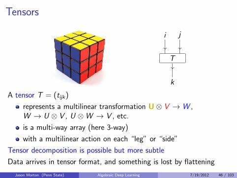
Tensors
T
��
i
��
j
k
��
A tensor T = (tijk)
represents a multilinear transformation U⊗ V → W ,W → U ⊗ V , U ⊗W → V , etc.
is a multi-way array (here 3-way)
with a multilinear action on each “leg” or “side”
Tensor decomposition is possible but more subtle
Data arrives in tensor format, and something is lost by flattening
Jason Morton (Penn State) Algebraic Deep Learning 7/19/2012 6 / 103

Example of tensor decompositionThree possible generalizations of eigenvalue decomposition are thesame in the matrix case but not in the tensor case. For a p × p × ptensor K ,
Name minimum r such that
Tensor rank K =∑r
i=1 ui ⊗ vi ⊗ wi
not closed
Border rank K = limε→0(Sε), Tensor rank(Sε) = rclosed but hard to represent;defining equations unknown.
Multilinear rank K = A · C ,C ∈ Rr×r×r ,A ∈ Rp×r ,closed and understood.
Jason Morton (Penn State) Algebraic Deep Learning 7/19/2012 7 / 103

Matrices vs Tensors
Generalization of matrix concepts to tensors is usually notstraightforward, but
flattenings are still matrices
effective computations in multilinear algebra generally reduce tolinear algebra (so far)
Jason Morton (Penn State) Algebraic Deep Learning 7/19/2012 8 / 103

Flatten
T
��
U
��
VW
��
Z
��
T
��
U
��
V
��
W
��
Z
View T ∈ U⊗V⊗W⊗Z as T : Z ∗⊗W ∗ → U⊗V
Jason Morton (Penn State) Algebraic Deep Learning 7/19/2012 9 / 103
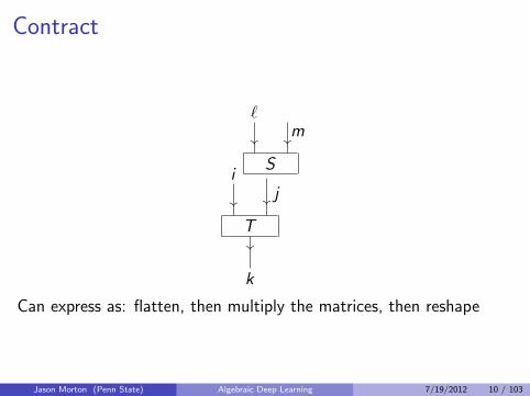
Contract
T
��
i
��j
k
��
S
��
`
��m
Can express as: flatten, then multiply the matrices, then reshape
Jason Morton (Penn State) Algebraic Deep Learning 7/19/2012 10 / 103

Algebraic geometry of tensor networks
Jason Morton (Penn State) Algebraic Deep Learning 7/19/2012 11 / 103

1 Algebraic geometry of tensor networksTensorsTensor NetworksAlgebraic geometry
2 Algebraic Description of Graphical ModelsReview of GM DefininitionsAlgebraic and semialgebraic descriptionsRestricted Boltzmann machines
3 Identifiability, singular learning theory, other perspectivesIdentifiabilitySingular Learning Theory
Jason Morton (Penn State) Algebraic Deep Learning 7/19/2012 12 / 103
What is a tensor network?
Jason Morton (Penn State) Algebraic Deep Learning 7/19/2012 13 / 103

And why do they keep coming up?
Bayesian networks: directed factor graph models
Converting a Bayesian network (a) to a directed factor graph (b).Factor f is the conditional distribution py |x , g is pz|x , and h is pw |z,y .
X Y
Z W
X f
g
Y
Z h
W
e
f
g
h
XY
ZW
(a) (b) (c)
(c) is a string diagram for a type of monoidal category; most of therest of the talk will be defining this.
Jason Morton (Penn State) Graphical models as monoidal categories 1/4/2012 5 / 25
When we reason about processes in space and time, involvinginteraction and independence, causality and locality, we tend todraw diagrams (networks) involving boxes, wires, arrowsAttaching mathematical meaning to such a diagram
I allows us to quantitatively model real systems and to computeI usually leads to defining a monoidal category
Analyzing the monoidal category often means defining a functorto the category of vector spaces and linear transformations
Jason Morton (Penn State) Algebraic Deep Learning 7/19/2012 14 / 103

Tensor Networks
Category theory provides a succint and beautiful means toformalize ideas about such diagrams and their interpetations inapplied mathematics
But I’ll focus on diagrams in the category of vector spaces andlinear transformations, often called tensor networks
Fortunately, many of the same mathematical ideas work toanalyze these whether they occur in machine learning, statistics,computational complexity, or quantum information
Algebraic geometry and representation theory provide a powerfulset of tools to characterize and understand these objects as theyarise in . . .
Jason Morton (Penn State) Algebraic Deep Learning 7/19/2012 15 / 103

Tensor Networks
|0〉
|0〉
|0〉
H
H
H
H
H
|000〉+|111〉√2
ML and Statistics Complexity Theory Quantum Informationand Many-Body Systems
Bayesian networks: directed factor graph models
Converting a Bayesian network (a) to a directed factor graph (b).Factor f is the conditional distribution py |x , g is pz|x , and h is pw |z,y .
X Y
Z W
X f
g
Y
Z h
W
e
f
g
h
XY
ZW
(a) (b) (c)
(c) is a string diagram for a type of monoidal category; most of therest of the talk will be defining this.
Jason Morton (Penn State) Graphical models as monoidal categories 1/4/2012 5 / 25
Pfaffian circuit/kernel counting example
76540123NAE
76540123
NAE
76540123NAE
76540123NAE
76540123
5 6
1 3
10 9
8
7
2
4
11
12
# of satisfying assignments =
〈all possibile assignments, all restrictions〉 = αβ√
det(x + y)
4096-dimensional space (C2)⊗12 12× 12 matrix
Jason Morton (Penn State) Pfaffian Circuits 1/6/2012 5 / 58
21
=
tim
e
(a) (b)
=
time
FIG. 19. Left (a) the circuit realization (internal to the triangle) of the function fW of e.g. (23) which outputslogical-one given input |x1x2x3〉 = |001〉, |010〉 and |100〉 and logical-zero otherwise. Right (b) reversing time andsetting the output to |1〉 (e.g. post-selection) gives a network representing the W-state. The naıve realization of fWis given in Figure 21 with an optimized co-algebraic construction shown in Figure 21.
FIG. 20. Naıve CTNS realization of the familiar W-state |001〉+ |010〉+ |100〉. A standard (temporal) acyclic classicalcircuit decomposition in terms of the XOR-algebra realizes the function fW of three bits. This function is given arepresentation on tensors. As illustrated, the networks input is post selected to |1〉 to realize the desired W-state.
Example 22 (Network realization of |ψ〉 = |01〉 + |10〉 + αk|11〉). We will now design a network to realizethe state |01〉 + |10〉 + αk|11〉. The first step is to write down a function fS such that
fS(0, 1) = fS(1, 0) = fS(1, 1) = 1 (27)
and fS(00) = 0 (in the present case, fS is the logical OR-gate). We post select the network output on |1〉,which yields the state |01〉 + |10〉 + |11〉, see Figure 23(a). The next step is to realize a diagonal operator,that acts as identity on all inputs, except |11〉 which gets sent to αk|11〉. To do this, we design a function fdsuch that
fd(0, 1) = fd(1, 0) = fd(0, 0) = 0 (28)
and fd(1, 1) = 1 (in the present case, fd is the logical AND-gate). This diagonal, takes the form in Figure23(b). The final state |ψ〉 = |01〉 + |10〉 + αk|11〉 is realized by connecting both networks, leading to Figure23(c).
VI. PROOF OF THE MAIN THEOREMS
We are now in a position to state the main theorem of this work. Specifically, we have a constructivemethod to realize any quantum state in terms of a categorical tensor network.8 We state and prove thetheorem for the case of qubit. The higher dimensional case of qudits follows from known results that anyd-state switching function can be expressed as a polynomial and realized as a connected network [47, 86, 87].The theorem can be stated as
8 A corollary of our exhaustive factorization of quantum states into tensor networks is a new type of quantum networkuniversality proof. To avoid confusion, we point out that past universality proofs in the gate model already imply that thelinear fragment (Figure 3) together with local gates is quantum universal. However, the known universality results clearlydo not provide a method to factor a state into a tensor network! Indeed, the decomposition or factorization of a state into atensor network is an entirely different problem which we address here.
Jason Morton (Penn State) Algebraic Deep Learning 7/19/2012 16 / 103

Tensors and wiring diagrams
T
��
U
��
V
W
��
A multilinear operatorT : U ⊗ V → Wis a tensor
Draw a wire for each vector space (variable)
Box for each tensor (factor)
Arrows denote primal/dual
Jason Morton (Penn State) Algebraic Deep Learning 7/19/2012 17 / 103

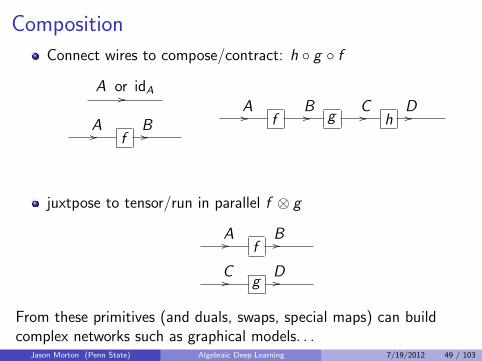
Composition
Connect wires to compose/contract: h ◦ g ◦ f
//A or idA
f//A
//B f//
Ag//
Bh//
C//D
juxtpose to tensor/run in parallel f ⊗ g
f//A
//B
g//C
//D
From these primitives (and duals, swaps, special maps) can buildcomplex networks
Jason Morton (Penn State) Algebraic Deep Learning 7/19/2012 18 / 103

You could have invented graphical models
This graphical notation has arisen several times in several areas(Feynman diagrams, graphical models, circuits, representationtheory. . . )
This convergent evolution is no accident and reflects anunderlying mathematical structure (monoidal categories)
Using the resulting common generalizations to study graphicalmodels is promising; makes translating results from/to otherareas much easier
Jason Morton (Penn State) Algebraic Deep Learning 7/19/2012 19 / 103
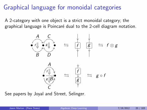
Graphical language for monoidal categories
A 2-category with one object is a strict monoidal category; thegraphical language is Poincare dual to the 2-cell diagram notation.
• •��A
II
B
f�� •��
C
II
D
g�� � f
��
��
g
��
��
� f ⊗ g
• •��
A
JJ
C
//
Bg��
f�� �
f
g
��
��
��
� g ◦ f
See papers by Joyal and Street, Selinger.
Jason Morton (Penn State) Algebraic Deep Learning 7/19/2012 20 / 103

Categories
A category C consists of a
class of objects Ob(C) and set Mor(A,B) of morphisms for eachordered pair of objects,
an associative composition rule taking morphisms Af→ B ,
Bg→ C , to a morphism g ◦ f : A→C
an identity idA ∈ Mor(A,A) such that idB ◦f = f = f ◦ idA.
Diagrammatically:
//A or idA
f//A
//B f//
Ag//
Bh//
C//D
Think of categories and variations as concrete and combinatorial.
Jason Morton (Penn State) Algebraic Deep Learning 7/19/2012 21 / 103

Monoidal categoriesDefinition
A monoidal category (C,⊗, α, λ, ρ, I) is a category C with theadditional data of
(i) an abstract tensor product functor ⊗ : C × C → C,
(ii) a natural isomorphism called the associatorαABC : (A⊗ B)⊗ C → A⊗ (B ⊗ C ),
(iii) a unit object I and natural isomorphisms λA : I⊗ A→ A andρA : A⊗ I, the left and right unitors,
such that if w ,w ′ are two words obtained from A1 ⊗ A2 ⊗ · · ·An byinserting Is and balanced parenthesis, then all isomorphismsφ : w → w ′ composed of αs, λs, and ρs and their inverses are equal.Thus we have a unique natural transformation w → w ′.
A monoidal category is strict if α, λ, and ρ are equalities. Monoidalcategories can be “strictified,” so the λ, ρ, α can often be ignored.
Jason Morton (Penn State) Algebraic Deep Learning 7/19/2012 22 / 103

Monoidal categories ctd.
DefinitionA monoidal category is braided if it is equipped with naturalisomorphisms bA⊗B : A⊗ B
∼→ B ⊗ A subject to the hexagon axiomsand symmetric if bA⊗BbB⊗A = idA⊗B .
Diagramatically:
=
braid isomorphismbA⊗B
symmetry relation
Jason Morton (Penn State) Algebraic Deep Learning 7/19/2012 23 / 103

From graphical model to string diagramQ: What does the graphical language of certain monoidal categorieswith additional axioms look like?A∗: Factor graph models.
X Y
Z W
X f
g
Y
Z h
W
e
f
g
h
XY
ZW
(a) (b) (c)
Converting a Bayesian network (a) to a directed factor graph (b) anda string diagram (c). Factor f is the conditional distribution py |x , g ispz|x , and h is pw |z,y .
Jason Morton (Penn State) Algebraic Deep Learning 7/19/2012 24 / 103

From graphical model to string diagram
•��� •???
◦
•
◦��� ◦???
◦
◦
◦→ →
Converting an undirected factor graph to a string diagram.
Jason Morton (Penn State) Algebraic Deep Learning 7/19/2012 25 / 103

Example: naıve Bayes
◦
•�������
• •???????
δA ◦ δA ◦ uA
A A A
B C D
A
B C D
Jason Morton (Penn State) Algebraic Deep Learning 7/19/2012 26 / 103

Example: gluing two triangles
••oooooo
•OOOOOO •oooooo
OOOOOO
C
A
B
D
A
B
δA
δB
C D
A
A A
B
B B
Jason Morton (Penn State) Algebraic Deep Learning 7/19/2012 27 / 103

RBM: Hadamard product of naıve Bayes
◦
•�������
• •???????
◦
????????
��������
A
B C D
E
B C DmB
mCmD
A
E
B C D
B C D
Jason Morton (Penn State) Algebraic Deep Learning 7/19/2012 28 / 103

Graphical models as tensor networks
Roughly
Wires are variables (Frobenius algebras)
Boxes are factors at fixed parameters, or spaces of factors asparameters vary
Under suitable assumptionsI global propertiesI (such as the set of equations cutting out the space of
representable probability distributions)I can be computed by gluing local properties
How do we describe these spaces of representable probabilitydistributions?
Jason Morton (Penn State) Algebraic Deep Learning 7/19/2012 29 / 103

Algebraic geometry of tensor networks
Jason Morton (Penn State) Algebraic Deep Learning 7/19/2012 30 / 103

1 Algebraic geometry of tensor networksTensorsTensor NetworksAlgebraic geometry
2 Algebraic Description of Graphical ModelsReview of GM DefininitionsAlgebraic and semialgebraic descriptionsRestricted Boltzmann machines
3 Identifiability, singular learning theory, other perspectivesIdentifiabilitySingular Learning Theory
Jason Morton (Penn State) Algebraic Deep Learning 7/19/2012 31 / 103

What is algebraic geometry?Study of solutions to systems of polynomial equations
Consider the ring of multivariate polynomials f ∈ C[x1, . . . , xn],e.g. 3x22x4 − 5x33Any polynomial f ∈ C[x1, . . . , xn] has a zero locus
{v = (v1, . . . , vn) ∈ Cn : f (v) = 0}.
This is the variety V (f ) cut out by f . For one polynomial, thisvariety is a hypersurface.
Introduction to Algebraic Geometry
Let R[p] = R[p1, . . . ,pm] be the set of all polynomials in indeterminatesp1, . . . ,pm with real coefficients.
DefinitionLet F ⊂ R[p1, . . . ,pm]. The variety defined by F is the set
V (F) := {a ∈ Rm | f (a) = 0 for all f ∈ F} .
V ({p2−p21}) =
Seth Sullivant (NCSU) Algebraic Statistics June 9, 2012 2 / 34
Jason Morton (Penn State) Algebraic Deep Learning 7/19/2012 32 / 103

What is algebraic geometry?
Study of solutions to systems of polynomial equations
Consider the ring of multivariate polynomials f ∈ C[x1, . . . , xn],e.g. 3x22x4 − 5x33Any polynomial f ∈ C[x1, . . . , xn] has a zero locus
{v = (v1, . . . , vn) ∈ Cn : f (v) = 0}.
This is the variety V (f ) cut out by f . For one polynomial, thisvariety is a hypersurface.
For example, the set of probability distributions that can berepresented by an RBM with 4 visible and 2 hidden nodes is partof a hypersurface.
I its f has degree 110 and probably around 5 trillion monomials[Cueto-Yu]
Jason Morton (Penn State) Algebraic Deep Learning 7/19/2012 33 / 103

Varieties defined by sets of polynomials
Now suppose you have a set F of polynomials: a system ofpolynomial equations
Requiring them all to hold simultaneously means we keep onlythe points where they all vanish:
I the intersection of their hypersurfaces
The zero locus
{v = (v1, . . . , vn) ∈ Cn : f (v) = 0 for all f ∈ F}
of a set of polynomials F is the variety V (F).
Jason Morton (Penn State) Algebraic Deep Learning 7/19/2012 34 / 103

Sets of polynomials defined by varieties
On the other hand,
Given a set S ⊂ Cn, the vanishing ideal of S is
I (S) = {f ∈ C[x1, . . . , xn] : f (a) = 0 ∀a ∈ S}.
Hilbert’s basis theorem: such an ideal has a finite generating set.
Combining these operations:a set S ⊂ Cn has a Zariski closure V (I (S)).
Jason Morton (Penn State) Algebraic Deep Learning 7/19/2012 35 / 103

Why applied algebraic geometry
“Any sufficiently advanced field of mathematics can model anyproblem.”
I Algebraic geometry is as old as it gets.
More formally:I Ideal membership / computing Grobner bases is
EXPSPACE-complete.I Matiyasevich’s theorem: every recursively enumerable set is a
Diophantine set (10th)
So any question with a computable answer can be phrased interms of algebraic geometry.
I If done well, get geometric insight into the problem and deephammers.
Jason Morton (Penn State) Algebraic Deep Learning 7/19/2012 36 / 103

Implicitization
We would like to study e.g. the space of probability distributionsrepresentable by various deep learning models.
These models are not given as sets of polynomials FThey are given in terms of a parameterization described by agraph: each box in the tensor network is allowed to be a certainrestricted set of tensors
So we need to study the map from parameter space toprobability space, its fibers, and its image.
A complete description tells us what equations and whatinequalities a probability distribution must satisfy in order tocome from, say, a DBN
Jason Morton (Penn State) Algebraic Deep Learning 7/19/2012 37 / 103

Implicitization
Define a polynomial map φ from a parameter space Θ ⊂ Cn toan ambient space Cm
x = t
y = t2
Defines an image φ(Θ) ⊂ Cm. What equations define, or cutout this set? y − x2 = 0 cuts out the image.
We took a Zariski closure
The process of finding defining equations of the image is calledimplicitization
This is hard! But not impossible.
Jason Morton (Penn State) Algebraic Deep Learning 7/19/2012 38 / 103

Example: Mixture of products
A
B C D
Jason Morton (Penn State) Algebraic Deep Learning 7/19/2012 39 / 103
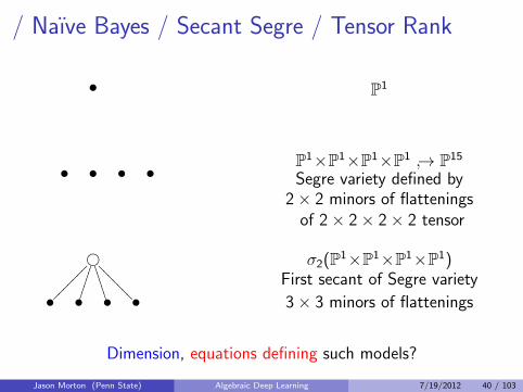
/ Naıve Bayes / Secant Segre / Tensor Rank
• P1
• P1×P1×P1×P1 ↪→ P15
Segre variety defined by2× 2 minors of flattenings
of 2× 2× 2× 2 tensor
• • •
��������•�������
•�����
•*****
•??????? σ2(P1×P1×P1×P1)First secant of Segre variety
3× 3 minors of flattenings
Dimension, equations defining such models?
Jason Morton (Penn State) Algebraic Deep Learning 7/19/2012 40 / 103

Computational Algebraic Geometry
There are computational tools for algebraic geometry, and manyadvances mix computational experiments and theory.
Grobner basis methods power general purpose software:Singular, Macaulay 2, CoCoA, (Mathematica, Maple)
I Symbolic term rewriting
Polyhedral methods (e.g. polymake, gfan) for certain problems;e.g. using work by Cueto and Yu, Bray and M- reduceimplicitization to (very) large-scale linear algebra: just find the(1d) kernel of a 5 trillion × 5 trillion matrix for RBM4,2.
Computational algebraic geometry computations now routinelyburn millions of CPU-hours of cluster compute time (e.g.implicitization, searching for efficiently contractable networks).
Jason Morton (Penn State) Algebraic Deep Learning 7/19/2012 41 / 103

Numerical Algebraic Geometry
Salmon Problem: Determine the ideal defining the fourth secantvariety of P3xP3xP3. Set theoretic [Friedland 2010], furtherprogress [Bates, Oeding 2010], [Friedland, Gross 2011].
Numerical Algebraic Geometry: Numerical methods forapproximating complex solutions of polynomial systems.
I Homotopy continuation (numerical path following).I Can be used to find isolated solutions or points on each
positive-dimensional irreducible component.I Can scale to thousands of variables for certain problems.I Reliable, parallelized, adaptive multiprecision software is
available: Bertini (Bates, Hauenstein, Sommese, and Wampler).
Jason Morton (Penn State) Algebraic Deep Learning 7/19/2012 42 / 103
Why are geometers interested?
Applications (especially tensor networks in statistics and CS)have revived classical viewpoints such as invariant theory.
Re-climbing the hierarchy of languages and tools (Italian school,Zariski-Serre, Grothendieck) as applied problems are unified andrecast in more sophisticated language.
Applied problems have also revealed gaps in our knowledge ofalgebraic geometry and driven new theoretical developments andcomputational tools
I Objects which are “large”: high-dimensional, many points, butwith many symmetries
I These often stabilize in some sense for large n.
Jason Morton (Penn State) Algebraic Deep Learning 7/19/2012 43 / 103

Lectures 2 and 3
Jason Morton (Penn State) Algebraic Deep Learning 7/19/2012 44 / 103

Last time
Last time, we talked about the
algebraic geometry of tensor networks
and how to learn something about this geometry
Jason Morton (Penn State) Algebraic Deep Learning 7/19/2012 45 / 103
Tensors
T
��
i
��
j
k
��
A tensor T = (tijk)
represents a multilinear transformation U⊗ V → W ,W → U ⊗ V , U ⊗W → V , etc.
is a multi-way array (here 3-way)
with a multilinear action on each “leg” or “side”
Tensor decomposition is possible but more subtle
Data arrives in tensor format, and something is lost by flattening
Jason Morton (Penn State) Algebraic Deep Learning 7/19/2012 46 / 103

One way things get harder with tensorsWhich tensor products Cd1 ⊗ · · · ⊗ Cdn have finitely many orbitsunder GL(d1,C)× · · · × GL(dn,C)?The answer for matrices is easyKac (1980), Parfenov (1998, 2001): up to C2 ⊗ C3 ⊗ C6, orbitrepresentatives and abutment graph
Orbits and their closures in the spaces Ck1 ⊗ · · · ⊗ Ckr 91
presented in Fig. 1, where the indices of vertices of the graph correspond to theindices of orbits appearing in Theorem 6. The integers on the left-hand side arethe dimensions of the orbits.
At the end of § 2 we prove Theorem 11, which asserts that in all cases underconsideration in our paper the abutment graphs are subgraphs of the abutmentgraph for the case (2, 3, 6). This graph is presented in Fig. 2, where the indicesof vertices correspond to the indices of orbits in Theorem 8. The integers on theleft-hand side are the dimensions of the orbits in their dependence on n.
For clarity the results of this paper are collected in Table 0. In this table, foreach case (2, m, n) we indicate the number of orbits of GL2×GLm×GLn and thedegree of the generator for the algebra of invariants of the corresponding groupSL2×SLm×SLn; we also indicate the statements relating to the orbits and thegraphs of abuttings.
Table 0
No. Case (2,m, n)The numberof orbits of
GL2×GLm×GLndeg f
Assertion
on the orbits
Assertion on the
abutment graph
1 (2, 2,2) 7 4 Lemma 2 Theorem 11, Fig. 2
2 (2, 2,3) 9 6 Theorem 8 Theorem 11, Fig. 2
3 (2, 2,4) 10 4 Theorem 8 Theorem 11, Fig. 2
4 (2, 2, n), n � 5 10 0 Theorem 8 Theorem 11, Fig. 2
5 (2, 3,3) 18 12 Theorem 6 Theorem 11, Figs. 1, 2
6 (2, 3,4) 24 12 Theorem 8 Theorem 11, Fig. 2
7 (2, 3,5) 26 0 Theorem 8 Theorem 11, Fig. 2
8 (2, 3,6) 27 6 Theorem 8 Theorem 11, Fig. 2
9 (2, 3, n), n � 7 27 0 Theorem 8 Theorem 11, Fig. 2
The main results of the present paper were published (without proofs) in [6].We use this opportunity to point out that [6] contains two disappointing mistakes,one of which is a consequence of the other. Namely:
(1) in Theorem 2, the line
(2, 2, n), n � 4, has ten orbits with representatives 1–9, 19
must be replaced by the line
(2, 2, n), n � 4, has ten orbits with representatives 1–7, 11, 13, 19;
(2) accordingly, the figure with the abutment graph should contain no arrowfrom vertex 19 to vertex 9, but there should be an arrow from the vertex 19 tovertex 13 instead.
I would like to express my deep gratitude to my research supervisor E. B. Vinbergfor setting the problem, crucial advice, and constant attention to this research.
Jason Morton (Penn State) Algebraic Deep Learning 7/19/2012 47 / 103

Another way
Consider a matrix turned into a vector
[x1, x2, x3, . . . x`]
can you compute its rank, SVD, kernel, etc?
Jason Morton (Penn State) Algebraic Deep Learning 7/19/2012 48 / 103
Composition
Connect wires to compose/contract: h ◦ g ◦ f
//A or idA
f//A
//B f//
Ag//
Bh//
C//D
juxtpose to tensor/run in parallel f ⊗ g
f//A
//B
g//C
//D
From these primitives (and duals, swaps, special maps) can buildcomplex networks such as graphical models. . .
Jason Morton (Penn State) Algebraic Deep Learning 7/19/2012 49 / 103

Tensor networks
X Y
Z W
X f
g
Y
Z h
W
e
f
g
h
XY
ZW
Jason Morton (Penn State) Algebraic Deep Learning 7/19/2012 50 / 103

Algebraic geometry
Study of solutions to systems of polynomial equations
Ring of multivariate polynomials f ∈ C[x1, . . . , xn], e.g.3x22x4 − 5ix33The zero locus
{v = (v1, . . . , vn) ∈ Cn : f (v) = 0 for all f ∈ F}
of a set of polynomials F is the variety V (F).
Given a set S ⊂ Cn, the vanishing ideal of S is
I (S) = {f ∈ C[x1, . . . , xn] : f (a) = 0 ∀a ∈ S}.
Hilbert’s basis theorem: such an ideal has a finite generating set.
A set S ⊂ Cn has a Zariski closure V (I (S)).
Jason Morton (Penn State) Algebraic Deep Learning 7/19/2012 51 / 103

Implicitization
Define a polynomial map φ from a parameter space Θ ⊂ Cn toan ambient space Cm
x = t
y = t2
Defines an image φ(Θ) ⊂ Cm. What equations define, or cutout this set? y − x2 = 0 cuts out the image.
We took a Zariski closure
The process of finding defining equations of the image is calledimplicitization
Jason Morton (Penn State) Algebraic Deep Learning 7/19/2012 52 / 103

Algebraic geometry and tensor networks
To an algebraic geometer, a tensor network
appearing in machine learning (statistics, signal processing,computational complexity, quantum computation, . . . )
describes a regular map φ from the parameter space (choice oftensors at the nodes) to an ambient space.
The image of φ is an algebraic variety of representableprobability distributions,
The fibers tell us about identifiability, transferability, andlearning rate
Jason Morton (Penn State) Algebraic Deep Learning 7/19/2012 53 / 103

1 Algebraic geometry of tensor networksTensorsTensor NetworksAlgebraic geometry
2 Algebraic Description of Graphical ModelsReview of GM DefininitionsAlgebraic and semialgebraic descriptionsRestricted Boltzmann machines
3 Identifiability, singular learning theory, other perspectivesIdentifiabilitySingular Learning Theory
Jason Morton (Penn State) Algebraic Deep Learning 7/19/2012 54 / 103

Algebraic description of probabilistic models
“Statistical models are algebraic varieties”
What distributions can be represented by a (graphical) model?
What is the geometry of the parameterization map?
Implications for approximation and optimization (learning)performance?
Jason Morton (Penn State) Algebraic Deep Learning 7/19/2012 55 / 103

Hierarchical models, undirected graphical models
Model joint probability distributions on N random variablesX1, . . . ,XN with finitely many states d1, . . . , dN .
Define dependence locally by a simplicial complex on{1, 2, . . . ,N}, parameterizing a family of probability distributionsby potential functions or factors, one per maximal simplex.
In an undirected graphical model, the simplicial complex is theclique complex of an undirected graph.
•A
•������
C
•D
•//////
B •��� •???
•
•
•��
•��
•
//
•//
UGM FG FG
Jason Morton (Penn State) Algebraic Deep Learning 7/19/2012 56 / 103

Hierarchical models: probability distribution
Model joint probability distributions on N random variablesX1, . . . ,XN with finitely many states d1, . . . , dN .
Define dependence locally by a simplicial complex on{1, 2, . . . ,N}, parameterizing a family of probability distributionsby potential functions or factors, one per maximal simplex.
In an undirected graphical model, the simplicial complex is theclique complex of an undirected graph.
Defines a family of probability distributions on discrete randomvariables X1, . . . ,XN , where Xi has di states by (before marginalizing)
pM(x) =1
Z
∏
s∈SΞs(xs)
where xs is the state vector restricted to the vertices in s, each Ξs isa tensor corresponding to the factor associated to simplex s.
Jason Morton (Penn State) Algebraic Deep Learning 7/19/2012 57 / 103

Hierarchical models: undirected factor graph models
A hierarchical model defines a factor graph, which is a bipartite graphΓ = (V ∪ H ,F ,E ) of nodes, factors and edges.
Each i ∈ {1, . . . ,N} = H ∪ V is labeled by a random variable Xi
and denoted by a open ◦ or filled • disc according to whether itis Hidden (latent) or Visible respectively.
Each maximal simplex s ∈ S is denoted by a box fs labeled by afactor fs ∈ F , and is connected by an edge to each variable discXi where i ∈ s.
•A
•������
C
•D
•//////
B •��� •???
•
•
•��
•��
•
//
•//
•��� •???
◦
•hidden
������
UGM FG FG FG
Jason Morton (Penn State) Algebraic Deep Learning 7/19/2012 58 / 103

Implicitization and graphical models
The Hammersley-Clifford Theorem is a theorem aboutimplicitizing undirected graphical models
They delayed publication for years trying to address thenonnegative case
This was completed in [Geiger, Meek, Sturmfels 2006] bystudying the algebraic geometry of these models (“AlgebraicStatistics”)
Jason Morton (Penn State) Algebraic Deep Learning 7/19/2012 59 / 103

Bayesian networks: directed factor graph models
A (discrete) Bayesian network M = (H ,V , d ,G ) is based on adirected acyclic graph G .
Vertices partitioned [N] = H ∪ V into hidden and visiblevariables; each variable i ∈ [N] has a number di of states.
The parameterization defines for each variable x a conditionalprobability distribution (a singly stochastic matrix) p(xi |xpa(i))where pa(i) is the set of vertices which are parents of i .
ThenpM(v) =
∑
xH
∏
i∈[N]
p(xi |xpa(i))
with p(xi |xpa(i)) ≥ 0,∑
i p(xi |xpa(i)) = 1 and no globalnormalization is needed because of the local normalization.
Jason Morton (Penn State) Algebraic Deep Learning 7/19/2012 60 / 103

Bayesian networks: directed factor graph models
Every Bayesian network can be written as a directed factorgraph model, but not conversely [Frey 2003].
Algebraic geometry of Bayesian networks [Garcia, Stillman,Sturmfels 2005]
Jason Morton (Penn State) Algebraic Deep Learning 7/19/2012 61 / 103

“Unhidden” Binary Deep Belief NetworkConsider a binary DBN with layer widths n0, . . . , n`. An “unhidden”binary DBN defines joint probability distributions of the form
P(h0, h1, . . . , h`) = P(h`−1, h`)`−2∏
k=0
P(hk |hk+1) ,
P(hk |hk+1) =
nk∏
j=1
P(hkj |hk+1) ,
P(hkj |hk+1) ∝ exp
(hkj b
kj + hkj
nk+1∑
i=1
W k+1j ,i hk+1
i
),
hk = (hkj )j ∈ {0, 1}nk is the state of the units in the kth layer,
W kj ,i ∈ R is the connection weight between the units j and i
from the (k − 1)th and kth layer respectively, and
bkj ∈ R is the bias weight of the jth unit in the kth layer.
Jason Morton (Penn State) Algebraic Deep Learning 7/19/2012 62 / 103
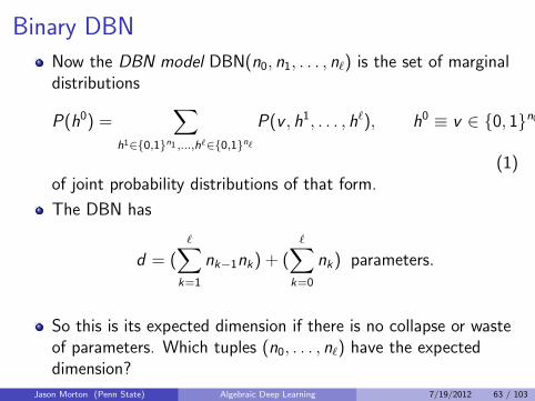
Binary DBN
Now the DBN model DBN(n0, n1, . . . , n`) is the set of marginaldistributions
P(h0) =∑
h1∈{0,1}n1 ,...,h`∈{0,1}n`P(v , h1, . . . , h`), h0 ≡ v ∈ {0, 1}n0
(1)of joint probability distributions of that form.
The DBN has
d = (∑
k=1
nk−1nk) + (∑
k=0
nk) parameters.
So this is its expected dimension if there is no collapse or wasteof parameters. Which tuples (n0, . . . , n`) have the expecteddimension?
Jason Morton (Penn State) Algebraic Deep Learning 7/19/2012 63 / 103

Where we are
The DBN contains many of the known models, hence
Don’t have a complete semialgebraic description of DBN, DBM.
Have partial information about representational power
Have algebraic, semialgebraic descriptions of submodels: naıveBayes, HMM, trees, RBM, etc.
I In some cases (especially small number of states), this is doneI In others, just have coarse information (dimension, relative
power)
Translating that understanding to something prescriptive isongoing
Let’s look at some of these submodels
Jason Morton (Penn State) Algebraic Deep Learning 7/19/2012 64 / 103

Naıve Bayes / Secant Segre / Tensor Rank
A
B C D
Jason Morton (Penn State) Algebraic Deep Learning 7/19/2012 65 / 103

Naıve Bayes / Secant Segre / Tensor RankLook at one hiden node in such a network, binary variables
• P1
• P1×P1×P1×P1 ↪→ P15
Segre variety defined by2× 2 minors of flattenings
of 2× 2× 2× 2 tensor
• • •
��������•�������
•�����
•*****
•??????? σ2(P1×P1×P1×P1)First secant of Segre variety
3× 3 minors of flattenings
Dimension, equations defining such models?
Jason Morton (Penn State) Algebraic Deep Learning 7/19/2012 66 / 103

Expected dimension of secant varieties
The expected dimension of σk(P1)n is
min(kn + k − 1, 2n − 1)
(e.g. by a parameter count)
But (especially for small n) things can collide and we can get adefect, where the dimension is less than expected
Dimension is among the first questions one can ask about avariety
I Is there hope for identifiability?I are there wasted parameters/ positive-dimensional fibers?I how big a model is needed to be able to represent all
distributions?
Jason Morton (Penn State) Algebraic Deep Learning 7/19/2012 67 / 103

Dimension of secant varieties
Recently [Catalisano, Geramita, Gimigliano 2011] showedσk(P1)n has the expected dimension
min(kn + k − 1, 2n − 1)
except σ3(P1)4 where it is 13 not 14.
Progress in Palatini 1909, . . . , Alexander Hirschowitz 1995,2000, CGG 2002,03,05, Abo Ottaviani Peterson 2006, Draisma2008, others.
Classically studied, revived by applications to statistics, quantuminformation, and complexity; shift to higher secants, solution.
So a generic tensor of (C2)⊗n can be written as a sum of d 2n
n+1e
decomposable tensors, no fewer.
Jason Morton (Penn State) Algebraic Deep Learning 7/19/2012 68 / 103

Representation theory of secant varieties
Raicu (2011) proved the ideal-theoretic GSS [Garcia StillmanSturmfels 05] conjecture
Equations defining σ2(Pk1 × · · · × Pkn)
Using representation theory of ideal of σ2(Pk1 × · · · × Pkn) as aGLk1 × · · ·GLkn-module
(progress in [Landsberg Manivel 04, Landsberg Weyman 07,Allman Rhodes 08]).
SECANT VARIETIES OF SEGRE–VERONESE VARIETIES 15
Definition 3.14. Given a partition µ = (µ1, · · · , µt) ` r, an n-partition λ `n r and a block
M ∈ Udµ , we associate to the element cλ ·M ∈ cλ · Udµ the n-tableau
T = (T 1, · · · , Tn) = T 1 ⊗ · · · ⊗ Tn
of shape λ, obtained as follows. Suppose that the block M has the set αij in its i-th row and
j-th column. Then we set equal to i the entries in the boxes of T j indexed by elements ofαij (recall from Section 2.3 that the boxes of a tableau are indexed canonically: from left to
right and top to bottom). Note that each tableau T j has entries 1, · · · , t, with i appearingexactly µi · dj times.
Note also that in order to construct the n-tableau T we have made a choice of the orderingof the rows of M : interchanging rows i and i′ when µi = µi′ should yield the same element
M ∈ Udµ , therefore we identify the corresponding n-tableaux that differ by interchangingthe entries equal to i and i′.
Example 3.15. We let n = 2, d = (2, 1), r = 4, µ = (2, 2) as in Example 3.2, and considerthe 2-partition λ = (λ1, λ2), with λ1 = (5, 3), λ2 = (2, 1, 1). We have
cλ ·1, 6 12, 3 44, 5 27, 8 3
1 2 2 3 31 4 4
⊗1 342
cλ ·2, 3 47, 8 31, 6 14, 5 2
3 1 1 4 43 2 2
⊗3 421
Let’s write down the action of the map πµ on the tableaux pictured above
πµ
1 2 2 3 3
1 4 4⊗
1 342
= 1 1 1 2 2
1 2 2⊗
1 221
+ 1 2 2 1 11 2 2
⊗1 122
+ 1 2 2 2 21 1 1
⊗1 212
.
We collect in the following lemma the basic relations that n-tableaux satisfy.
Lemma 3.16. Fix an n partition λ `n r, and let T be an n-tableau of shape λ. Thefollowing relations hold:
(1) If σ is a permutation of the entries of T that preserves the set of entries in eachcolumn of T , then
σ(T ) = sgn(σ) · T.In particular, if T has repeated entries in a column, then T = 0.
Jason Morton (Penn State) Algebraic Deep Learning 7/19/2012 69 / 103

Equations of the naive Bayes model (secant
varieties of Segre varieties)
Good news/bad news
Good News: We know them for small number of states
Bad News: But we don’t know them for large numbers of states.
Good News: In some cases, just minors of flattenings
Bad News: But not in general.
Good News: Many models (trees, RBM, DBN) are built bygluing naıve Bayes models together, so we have someinformation and the good news above propagates
Bad News: But so does the bad news.
Jason Morton (Penn State) Algebraic Deep Learning 7/19/2012 70 / 103

Algebraic description of Hidden Markov Models
A simplified (circular) version. Fix parameter matrices A1, . . . ,Ad .Then up to a global rescaling,
p =∑
i1,...,in
tr(Ai1 · · ·Ain)ei1i2···in
Jason Morton (Penn State) Algebraic Deep Learning 7/19/2012 71 / 103

Algebraic description of Hidden Markov Models
A simplified (circular) version. Fix parameter matrices A1, . . . ,Ad .Then up to a global rescaling,
p =∑
i1,...,in
tr(Ai1 · · ·Ain)ei1i2···in
What are the polynomial relations that hold among the coefficients
pi1,...in = tr(Ai1 · · ·Ain)?
That is, the ideal I = {f : f (pi1,...in) = 0} of polynomials f in thecoefficients such that f (pi1,...in) = 0.
Series of papers [Bray and M- 2006], [Schonhuth 2008, 2011], [Critch2012] provide characterizations, membership tests, identifiability, etc.
Jason Morton (Penn State) Algebraic Deep Learning 7/19/2012 72 / 103
(Phylogenetic) Trees
Jason Morton (Penn State) Algebraic Deep Learning 7/19/2012 73 / 103

Trees
Jason Morton (Penn State) Algebraic Deep Learning 7/19/2012 74 / 103

Trees and the General Markov Model
Studied in a long series of papers by authors includingSturmfels-Sullivant, Casanellas, Draisma-Kuttler,Allman-Rhodes, many others
I Many techniques were developed first on this reasonablytractable class
Ideas include changes of coordinates (Fourier transform,cumulant coordinates), gluing constructions, hard work
Now have complete algebraic description of many special classes
Complete semi-algebraic description of GMM for small numberof states [Allman et al. 2012]
This is a submodel of the DBN.
Jason Morton (Penn State) Algebraic Deep Learning 7/19/2012 75 / 103

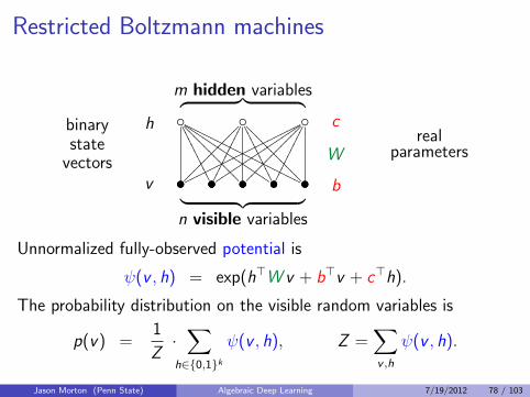
Restricted Boltzmann Machines
Jason Morton (Penn State) Algebraic Deep Learning 7/19/2012 76 / 103

pre-RBM: graphical model on a bipartite graph
•
• •/////////
•???????????
•JJJJJJJJJJJJJJ
•OOOOOOOOOOOOOOOOOO •
•�����������
•���������
• •/////////
•??????????? •
•oooooooooooooooooo
•tttttttttttttt
•�����������
•���������
•
binarystate
vectors
h
v
︷ ︸︸ ︷m variables
︸ ︷︷ ︸n variables
realparameters
c
b
W
Unnormalized potential is built from node and edge parameters
ψ(v , h) = exp(h>Wv + b>v + c>h).
The probability distribution on the binary random variables is
p(v , h) =1
Z·ψ(v , h), Z =
∑
v ,h
ψ(v , h).
Jason Morton (Penn State) Algebraic Deep Learning 7/19/2012 77 / 103
Restricted Boltzmann machines
◦
• •/////////
•???????????
•JJJJJJJJJJJJJJ
•OOOOOOOOOOOOOOOOOO ◦
•�����������
•���������
• •/////////
•??????????? ◦
•oooooooooooooooooo
•tttttttttttttt
•�����������
•���������
•
binarystate
vectors
h
v
︷ ︸︸ ︷m hidden variables
︸ ︷︷ ︸n visible variables
realparameters
c
b
W
Unnormalized fully-observed potential is
ψ(v , h) = exp(h>Wv + b>v + c>h).
The probability distribution on the visible random variables is
p(v) =1
Z·∑
h∈{0,1}kψ(v , h), Z =
∑
v ,h
ψ(v , h).
Jason Morton (Penn State) Algebraic Deep Learning 7/19/2012 78 / 103

Restricted Boltzmann machines
◦
• •/////////
•???????????
•JJJJJJJJJJJJJJ
•OOOOOOOOOOOOOOOOOO ◦
•�����������
•���������
• •/////////
•??????????? ◦
•oooooooooooooooooo
•tttttttttttttt
•�����������
•���������
•
binarystate
vectors
h
v
︷ ︸︸ ︷m hidden variables
︸ ︷︷ ︸n observed variables
realparameters
c
b
W
The restricted Boltzmann machine (RBM) is the undirectedgraphical model for binary random variables thus specified.
Denote by Mmn the set of joint distributions as
b ∈ Rn, c ∈ Rk ,W ∈ Rm×n vary.
Mmn is a subset of the probability simplex ∆2n−1.
Jason Morton (Penn State) Algebraic Deep Learning 7/19/2012 79 / 103

Hadamard Products of VarietiesGiven two projective varieties X and Y in P`, their Hadamardproduct X∗Y is the closure of the image of
X × Y 99K P` , (x , y) 7→ (x0y0 : x1y1 : . . . : x`y`).
We also define Hadamard powers X [m] = X ∗ X [m−1].
If M is a subset of the simplex ∆`−1 then M [m] is also defined bycomponentwise multiplication followed by rescaling so that thecoordinates sum to one. This is compatible with taking Zariski
closure: M [m] = M[m]
LemmaRBM variety and RBM model factor as
Vmn = (V 1
n )[m] and Mmn = (M1
n )[m].
Jason Morton (Penn State) Algebraic Deep Learning 7/19/2012 80 / 103

RBM as Hadamard product of naıve Bayes
◦
•�������
• •???????
◦
????????
��������
A
B C D
E
B C DmB
mCmD
A
E
B C D
B C D
Jason Morton (Penn State) Algebraic Deep Learning 7/19/2012 81 / 103

Representational power of RBMs
Conjecture
The restricted Boltzmann machine has the expected dimension.
That is, Mmn is a semialgebraic set of dimension
min{nm + n + m, 2n − 1} in ∆2n−1.
Jason Morton (Penn State) Algebraic Deep Learning 7/19/2012 82 / 103
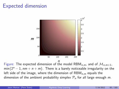
Expected dimension
50 100 150 200
150
100
50
0
0.5
1
1.5
2
2.5
3
3.5
4x 10
4
n
mm
Figure: The expected dimension of the model RBMn,m, and of Mn,m+1,min{2n − 1, nm + n + m}. There is a barely noticeable irregularity on theleft side of the image, where the dimension of RBMn,m equals thedimension of the ambient probability simplex Pn for all large enough m.
Jason Morton (Penn State) Algebraic Deep Learning 7/19/2012 83 / 103

Representational power of RBMs
We can show many special cases and the following general result:
Theorem (Cueto M- Sturmfels)
The restricted Boltzmann machine has the expected dimension
nm + n + m when m < 2n−dlog2(n+1)e
min{nm + n + m, 2n − 1} when m = 2n−dlog2(n+1)e and
2n − 1 when m ≥ 2n−blog2(n+1)c.
Covers most cases of restricted Boltzmann machines in practice,as those generally satisfy m ≤ 2n−dlog2(n+1)e.
Proof uses tropical geometry, coding theory
Jason Morton (Penn State) Algebraic Deep Learning 7/19/2012 84 / 103

Tropical RBM Model
Tropical geometry is the “polyhedral shadow” of algebraicgeometry.
The process of passing from ordinary arithmetic to the max-plusalgebra is known as tropicalization.
The tropicalization Φ of our RBM parameterization is the mapΦ : Rnm+n+m → TP2n−1 = R2n/R(1, 1, . . . , 1) whose 2n
coordinates are the tropical polynomials
qv = max{h>Wv + b>v + c>h : h ∈ {0, 1}m
}
This yields a piecewise-linear concave function Rnm+n+m → R onthe space of model parameters (W , b, c).
Its image TMmn is called the tropical RBM model.
Jason Morton (Penn State) Algebraic Deep Learning 7/19/2012 85 / 103

Tropical RBM Variety
The tropical hypersurface T (f ) is the union of all codimensionone cones in the normal fan of the Newton polytope of f .
The tropical RBM variety TVmn is the intersection in TP2n−1 of
all the tropical hypersurfaces T (f ) where f runs over allpolynomials that vanish on Vm
n (or on Mmn ).
Understand tropical variety, use:
dim(TMmn ) ≤ dim(TVm
n ) = dim(Vmn ) =
dim(Mmn ) ≤ min{nm + n + m, 2n − 1}
and coding theory to obtain the result.
Jason Morton (Penn State) Algebraic Deep Learning 7/19/2012 86 / 103

Relative representational power
Another way to study the representational power of RBMs andDBNs is to compare them with other models
When does one potential model contain another?
Jason Morton (Penn State) Algebraic Deep Learning 7/19/2012 87 / 103
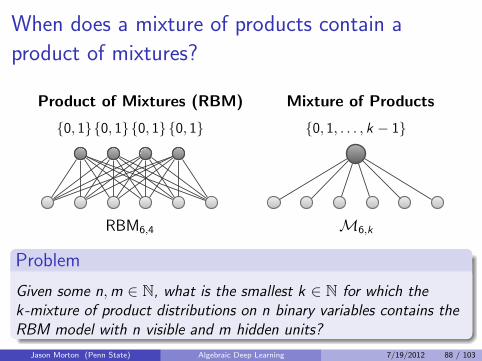
When does a mixture of products contain a
product of mixtures?
{0, 1}{0, 1}{0, 1}{0, 1} {0, 1, . . . , k − 1}Product of Mixtures (RBM) Mixture of Products
RBM6,4 M6,k
Problem
Given some n,m ∈ N, what is the smallest k ∈ N for which thek-mixture of product distributions on n binary variables contains theRBM model with n visible and m hidden units?
Jason Morton (Penn State) Algebraic Deep Learning 7/19/2012 88 / 103

Exponentially more efficientFrom Yoshua’s first talk
#2 The need for distributed representations
Mul%-‐ Clustering Clustering
18
Learning a set of features that are not mutually exclusive can be exponen%ally more sta%s%cally efficient than nearest-‐neighbor-‐like or clustering-‐like models
Jason Morton (Penn State) Algebraic Deep Learning 7/19/2012 89 / 103
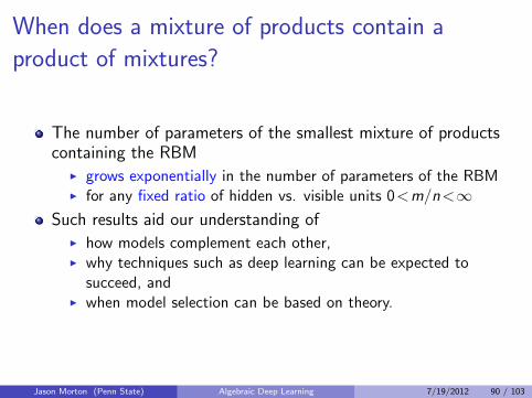
When does a mixture of products contain a
product of mixtures?
The number of parameters of the smallest mixture of productscontaining the RBM
I grows exponentially in the number of parameters of the RBMI for any fixed ratio of hidden vs. visible units 0<m/n<∞
Such results aid our understanding ofI how models complement each other,I why techniques such as deep learning can be expected to
succeed, andI when model selection can be based on theory.
Jason Morton (Penn State) Algebraic Deep Learning 7/19/2012 90 / 103
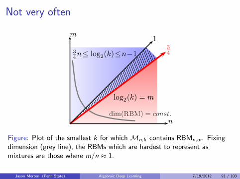
Not very often
m
n
log2(k) = m
34n≤ log2(k)≤n−1
34
1
dim(RBM) = const.
Figure: Plot of the smallest k for which Mn,k contains RBMn,m. Fixingdimension (grey line), the RBMs which are hardest to represent asmixtures are those where m/n ≈ 1.
Jason Morton (Penn State) Algebraic Deep Learning 7/19/2012 91 / 103

Modes and strong modes
Definition
Call x ∈ {0, 1}n a mode of p ∈ Pn if p(x) > p(x) for all x withdH(x , x) = 1, and a strong mode if p(x) >
∑x :dH(x ,x)=1 p(x).
One way to make precise that the RBM can represent morecomplicated distributions than a mixture model of similar size isto study this bumpiness in Hamming space.
On the one hand the sets of strong modes C⊂{0, 1}n realizableby a mixture model Mn,k are exactly the binary codes ofminimum Hamming distance two and cardinality at most k .
On the other hand. . .
Jason Morton (Penn State) Algebraic Deep Learning 7/19/2012 92 / 103

RBMs and Linear Threshold Codes
11
55
33
77
22
66
44
DefinitionA subset C ⊆ {0, 1}n is an (n,m)-linear threshold code (LTC) iffthere exist n linear threshold functions fi : {0, 1}m → {0, 1}, i ∈ [n]with
{(f1(x), f2(x), . . . , fn(x)) ∈ {0, 1}n : x ∈ {0, 1}m} = C.
If the functions fi can be chosen self-dual (hyperplanes are central),then C is called homogeneous.
Jason Morton (Penn State) Algebraic Deep Learning 7/19/2012 93 / 103

Strong modes and linear threshold codes
On the other hand,
for codes C ⊆ {0, 1}n, |C| = 2m of minimum distance two,
when C is a homogeneous linear threshold code (LTC)
then RBMn,m can represent a distribution with strong modes C.
And, if RBMn,m can represent a distribution with strong modesC, then C is a LTC.
Jason Morton (Penn State) Algebraic Deep Learning 7/19/2012 94 / 103

Combining these results gives our answer to
Problem
Given some n,m ∈ N, what is the smallest k ∈ N for which thek-mixture of product distributions on n binary variables contains theRBM model with n visible and m hidden units?
Namely, if 4dm/3e≤n, then Mn,k⊇RBMn,m if and only ifk≥2m;
and if 4dm/3e>n, then Mn,k⊇RBMn,m only ifk≥min{2l +m−l , 2n−1}, where l is max{l ∈ N : 4dl/3e≤n}.Thus an exponentially larger mixture model, with anexponentially larger number of parameters, is required torepresent distributions that can be represented by the RBM.
There’s another way to see that the RBM has points of rank 2m
when 2m ≤ n
Jason Morton (Penn State) Algebraic Deep Learning 7/19/2012 95 / 103

Not very often
m
n
log2(k) = m
34n≤ log2(k)≤n−1
34
1
dim(RBM) = const.
Figure: Plot of the smallest k for which Mn,k contains RBMn,m. Fixingdimension (grey line), the RBMs which are hardest to represent asmixtures are those where m/n ≈ 1.
Jason Morton (Penn State) Algebraic Deep Learning 7/19/2012 96 / 103

1 Algebraic geometry of tensor networksTensorsTensor NetworksAlgebraic geometry
2 Algebraic Description of Graphical ModelsReview of GM DefininitionsAlgebraic and semialgebraic descriptionsRestricted Boltzmann machines
3 Identifiability, singular learning theory, other perspectivesIdentifiabilitySingular Learning Theory
Jason Morton (Penn State) Algebraic Deep Learning 7/19/2012 97 / 103

Identifiability: uniqueness of parameter estimates
A parameterization of a set of probability distributions isidentifiable if it is injective.
A parameterization of a set of probability distributions isgenerically identifiable if it is injective except on a properalgebraic subvariety of parameter space.
Identifiability questions can be answered with algebraic geometry(e.g. many recent results in phylogenetics)
A weaker question: What conditions guarantee genericidentifiability up to known symmetries?
A still weaker question: is the dimension of the space ofrepresentable distributions (states) equal to the expecteddimension (number of parameters)? Or are parameters wasted?
Jason Morton (Penn State) Algebraic Deep Learning 7/19/2012 98 / 103

Uniqueness up to known symmetries and normal
forms
Identify internal symmetries (here SL2)
Reparameterize to choose a normal form
Jason Morton (Penn State) Algebraic Deep Learning 7/19/2012 99 / 103

Singular learning theoryA model is more than its implicitization; the parameterization map iscritically important to learning performance and quality.
How fast and how well can a model learn?
When a statistical model is regular, we can use central limittheorems to figure out their behavior for large data.
But most hidden variable models are not regular (identifiable w/positive definite Fisher information matrix) but singular.
Singular learning theory [Watanabe 2009] offers one avenue forprogress in this situation based on algebraic geometry.
Asymptotics, generalization error, etc are governed by the reallog canonical threshold.
Resolve the model singularities and develop new limit theorems.
Jason Morton (Penn State) Algebraic Deep Learning 7/19/2012 100 / 103

Comparing Architectures
/. -,() *+/. -,() *+
������������������������������������������������������������������������������������������������������������������������������������������������������������������������ ��
OO
/. -,() *+/. -,() *+
/. -,() *+/. -,() *+
��������������������������������������������������������������������������������
��������������������������������������������������������������������������������������������������������
OO��
��OO
��OO
RBM Treelike(9,18): 189 parameters (9,8,6,6): 185 parameters
/. -,() *+/. -,() *+
/. -,() *+
����������������������������������������������������������������������������������������������������������������
����������������������������������������������������������
OO
��OO
/. -,() *+/. -,() *+/. -,() *+
������������������������������������������������������������������������������������������������������������������������������������������������������������������������
��OO
��OO
Bulge Column(9,11,6): 191 parameters (9,9,9): 189 parameters
Jason Morton (Penn State) Algebraic Deep Learning 7/19/2012 101 / 103

Optimal architectures for learning
The real log canonical threshold λq of a parameterization at truedistribution q = p(x |θ) determines Bayes generalization error,
Gn(q) = Eq[KL(q||p∗n)]− Sq = λqn
+ o( 1n
) [Watanabe 2009].I Expected KL-divergenceI from the true model to the predicted distribution p∗
I after seeing n observations and updating to the posterior.
E.g. what do we have to believe about which qs appear innature for the deep model to be better, λRBM(q) > λCOL(q)?
Techniques for calculating λ are rapidly evolving; known forsimple binary graphical models such as trees [Zwiernik 2011].
Jason Morton (Penn State) Algebraic Deep Learning 7/19/2012 102 / 103

Advertisement
Modern applications of representation theoryI an IMA PI Graduate Summer SchoolI at the University of ChicagoI Summer 2014
≈ 12 Lectures on tensor networks
Jason Morton (Penn State) Algebraic Deep Learning 7/19/2012 103 / 103
Recommended


![arXiv:1705.06206v2 [math.QA] 5 Dec 2017 · spaces of states. We call the two-dimensional Hilbert space C2 with preferred basis j0iand j1i a qubit. Therefore, a qubit, utilizing superposition,](https://img.dokumen.tips/doc/110x75/5e6a34fd4dd0a8778a6b29c5/arxiv170506206v2-mathqa-5-dec-2017-spaces-of-states-we-call-the-two-dimensional.jpg)


