
AIRBORNE WIRELESS COMMUNICATION MODELING AND ANALYSIS
THESIS
Matthew J. Vincie, Lieutenant, USAF
AFIT-ENG-14-M-80
DEPARTMENT OF THE AIR FORCE AIR UNIVERSITY
AIR FORCE INSTITUTE OF TECHNOLOGY
Wright-Patterson Air Force Base, Ohio
DISTRIBUTION STATEMENT A. APPROVED FOR PUBLIC RELEASE; DISTRIBUTION UNLIMITED.

The views expressed in this thesis are those of the author and do not reflect the official policy or position of the United States Air Force, Department of Defense, or the United States Government. This material is declared a work of the U.S. Government and is not subject to copyright protection in the United States.

AFIT-ENG-14-M-80
AIRBORNE WIRELESS COMMUNICATION MODELING AND ANALYSIS
THESIS
Presented to the Faculty
Department of Electrical and Computer Engineering
Graduate School of Engineering and Management
Air Force Institute of Technology
Air University
Air Education and Training Command
In Partial Fulfillment of the Requirements for the
Degree of Master of Science in Electrical Engineering
Matthew J. Vincie, BS
Lieutenant, USAF
March 2014
DISTRIBUTION STATEMENT A. APPROVED FOR PUBLIC RELEASE; DISTRIBUTION UNLIMITED.

AFIT-ENG-14-M-80
AIRBORNE WIRELESS COMMUNICATION MODELING AND ANALYSIS
Matthew J. Vincie, BS
Lieutenant, USAF
Approved:
//signed// 13-03-14 Dr. Gilbert L. Peterson (Chairman) Date //signed// 13-03-14 Dr. John M. Colombi (Member) Date //signed// 13-03-14 Dr. David R. Jacques (Member) Date

iv
AFIT-ENG-14-M-80
Abstract
Over the past decade, there has been a dramatic increase in the use of unmanned
aerial vehicles (UAV) for military, commercial, and private applications. Critical to
maintaining control and a use for these systems is the development of wireless
networking systems [1]. Computer simulation has increasingly become a key player in
airborne networking developments though the accuracy and credibility of network
simulations has become a topic of increasing scrutiny [2-5]. Much of the inaccuracies
seen in simulation are due to inaccurate modeling of the physical layer of the
communication system. This research develops a physical layer model that combines
antenna modeling using computational electromagnetics and the two-ray propagation
model to predict the received signal strength. The antenna is modeled with triangular
patches and analyzed by extending the antenna modeling algorithm by Sergey Makarov,
which employs Rao-Wilton-Glisson basis functions. The two-ray model consists of a
line-of-sight ray and a reflected ray that is modeled as a lossless ground reflection.
Comparison with a UAV data collection shows that the developed physical layer model
improves over a simpler model that was only dependent on distance. The resulting two-
ray model provides a more accurate networking model framework for future wireless
network simulations.

v
I would like to thank my family and friends for their support in this endeavor. I would
also like to extend a special thanks to my fiancée for her thoughtfulness and
encouragement. Your love and support are very much appreciated.

vi
Acknowledgments
I would like to express my sincere appreciation to my advisor, Dr. Gilbert
Peterson, for his guidance and support throughout the course of my research. I would also
like to thank Dr. David Jacques and Dr. John Colombi for their invaluable training in
unmanned aerial systems and their involvement in flight-testing. I would like to thank
Rick Patton and Captain Charles Neal for their technical guidance and assistance with
flight tests. I would also like to thank the staff at Radical RC in Dayton, Ohio for their
advice and demonstration of wiring procedures. I would like to extend appreciation to
Co-Operative Engineering Services, Inc. (CESI) for facilitating the flight tests.
Matthew J. Vincie

vii
Table of Contents
Page
Abstract .............................................................................................................................. iv
Table of Contents .............................................................................................................. vii
List of Figures ......................................................................................................................x
I Introduction ..................................................................................................................1
1.2. Goals ......................................................................................................................2
1.3. Methodology..........................................................................................................2
1.4. Contribution ...........................................................................................................2
1.5. Results ...................................................................................................................3
1.6. Layout ....................................................................................................................3
II Literature Review .........................................................................................................4
2.1. Chapter Overview ..................................................................................................4
2.2 Reduction on DoD Electromagnetic Spectrum ......................................................4
2.3 Emergency Communications ..................................................................................5
2.4. Previous Research at AFIT using OPNET ............................................................5
2.5. Network Simulators ...............................................................................................6
2.6. Propagation Modeling: Ray Tracing .....................................................................7
2.7. Propagation Modeling: Statistical Models ............................................................8
2.8. Antenna Modeling .................................................................................................9
2.9. Scalar, Vector, and Matrix Notations ..................................................................10
2.10. Summary ............................................................................................................10
III Methodology ..............................................................................................................11
3.1. Chapter Overview ................................................................................................11

viii
3.2. Conversion of Aircraft GPS Location into the Local Cartesian Frame ...............14
3.3. Reflection Point Localization ..............................................................................15
3.4. Transformations between Orthogonal Coordinate Frames ..................................17
3.5. Transmitting Antenna Model ..............................................................................19
3.6. Reflection Modelling ...........................................................................................25
3.7. LOS Ray ..............................................................................................................30
3.8. Receiving Antenna Model ...................................................................................31
3.9. Validation Testing ...............................................................................................33
3.10. Performance Evaluation ....................................................................................40
3.11. Summary ............................................................................................................41
IV Analysis and Results ..................................................................................................43
4.1. Chapter Overview ................................................................................................43
4.2. Yaw Angle Correction .........................................................................................43
4.3. Results of Air-to-Air Scenario .............................................................................45
4.4. Results of Ground-to-Air Scenario ......................................................................49
4.5. Results of Air-to-Ground Scenario ......................................................................51
4.6. Combined Result of All Scenarios ......................................................................52
4.7. Summary..............................................................................................................56
V Conclusions and Recommendations ...........................................................................58
5.1. Chapter Overview ................................................................................................58
5.2. Justification for Research ....................................................................................58
5.3. Research Goals ....................................................................................................58
5.4. Research Contribution .........................................................................................59

ix
5.5. Conclusions of Research .....................................................................................59
5.6. Significance of Research .....................................................................................61
5.7. Recommendations for Future Research ...............................................................61
Appendix A. Hardware Configuration ...............................................................................63
A.1. Aircraft................................................................................................................63
A.2. Client Aircraft Payload Configuration ...............................................................66
A.3. Access Point Aircraft Payload Configuration ....................................................72
A.4. Using APM autopilot feature ..............................................................................73
Appendix B. Software Configuration ................................................................................75
B.1. ArduPlane source code modifications ................................................................75
B.2. WLAN module setup process .............................................................................79
B.3. Troubleshooting configuration ...........................................................................84
Appendix C. Access point Configuration Parameters. ......................................................86
Appendix D. Client Configuration Parameters ..................................................................88
Appendix E. Supporting Figures........................................................................................90
E.1. Air-to-Air Scenario Figures ................................................................................90
E.2. Ground-to-Air Scenario Figures .........................................................................98
E.3. Air-to-Ground Scenario Figures .......................................................................110
E.4. Figures from all scenarios combined ................................................................122
Bibliography ....................................................................................................................126

x
List of Figures
Page
Figure 1: Seven Layer OSI Model [11]. ............................................................................. 6
Figure 2: OPNET Radio Transceiver Pipeline [36] ............................................................ 7
Figure 3: Airborne Two-Ray Model. ................................................................................ 11
Figure 4: Two-Ray Algorithm Flow Chart (Part 1 of 2). .................................................. 12
Figure 5: Two-Ray Algorithm Flow Chart (Part 2 of 2). .................................................. 13
Figure 6: Map of Small UAV Airstrip Superimposed with Local Frame. ........................ 15
Figure 7: Reflection Geometry in Local Frame. ............................................................... 16
Figure 8: Plane of Incidence Geometry. ........................................................................... 17
Figure 9: Antenna's Coordinate Frame. ............................................................................ 18
Figure 10: Internal Geometry of Research Antenna. ........................................................ 20
Figure 11: 3-D Antenna Model made from 2-D Patches. ................................................. 21
Figure 12: Qualitative Representation of Power Distribution. ......................................... 22
Figure 13: Vertical Plane Co-polarization E-field Pattern (Radial Unit is dB). ............... 23
Figure 14: Vertical Plane Power Pattern (Radial Unit is dB). .......................................... 24
Figure 15: Horizontal Plane H-field Co-polarization Pattern (Radial Unit is dB). .......... 24
Figure 16: Reflection Coordinate Frame Shown in Local Frame. .................................... 26
Figure 17: View from above xy-plane. ............................................................................. 27
Figure 18: Plane of Incidence View. ................................................................................. 28
Figure 19: Incidence Model Geometry. ............................................................................ 32
Figure 20: Test Setup 1 for Vertical Plane Power Pattern Analysis. ................................ 33
Figure 21: Validation Vertical Plane Power Pattern. ........................................................ 34

xi
Figure 22: Test Setup 2 for Vertical Plane Power Pattern Analysis. ................................ 34
Figure 23: Test Setup for Polarization Mismatch Analysis. ............................................. 35
Figure 24: Simulated and Theoretical RSS vs. Polarization Mismatch Angle. ................ 36
Figure 25: RSS vs. Distance (Height = 1.50 m and Vertical Polarization). ..................... 38
Figure 26: RSS vs. Distance (Height = 1.50 m and Horizontal Polarization). ................. 39
Figure 27: RSS Pattern Produced by Interference (Height = 1.50 m and V-Pol.). ........... 40
Figure 28: Flight Path Overlaid with Antenna’s Frame using Autopilot Yaw. ................ 44
Figure 29: Flight Path Overlaid with Antenna’s Frame using GPS Based Yaw. ............. 45
Figure 30: Statistical Analysis of AtoA Scenario with Raw Heading. ............................. 47
Figure 31: Snapshot of RSS vs. Time for AtoA Scenario using Raw Heading. ............... 48
Figure 32: Statistical Analysis of GtoA Scenario with Raw Heading. ............................. 50
Figure 33: Statistical Analysis of AtoG Scenario with Raw Heading. ............................. 51
Figure 34: Statistical Analysis of All Scenarios with Raw Heading. ............................... 52
Figure 35: Elevation Angle Geometry. ............................................................................. 53
Figure 36: Error Statistics of All Scenarios with respect to Elevation Angle. ................. 55
Figure 37: Bias of Errors and Mean Absolute Value of Elevation Angle vs. Distance .... 56
Figure 38: Amplitude of Electric Field in the Direction of Propagation vs. Distance. ..... 60
Figure 39: Elevator Servo. ................................................................................................ 64
Figure 40: Rudder Servo. .................................................................................................. 64
Figure 41: Servo connections for wings. .......................................................................... 65
Figure 42: Spektrum receiver with externally mounted remote receiver. ........................ 65
Figure 43: RN-171-XV connected directly to antenna. .................................................... 67
Figure 44: Image of payload bay. ..................................................................................... 68

xii
Figure 45: Diagram of payload components for the client aircraft. .................................. 69
Figure 46: GPS/magnetometer module and antenna. ....................................................... 70
Figure 47: Side view displaying antenna placement. ........................................................ 70
Figure 48: UART2 connection.......................................................................................... 71
Figure 49: WLAN module connection. ............................................................................ 72
Figure 50: Diagram of payload for access point aircraft. ................................................. 73
Figure 51: Failsafe mux implementation. ......................................................................... 74
Figure 52: Serial port selection in Tera Term. .................................................................. 80
Figure 53: Message seen on startup. ................................................................................. 81
Figure 54: Setting baud rate for serial port. ...................................................................... 82
Figure 55: Message received from client module on startup. ........................................... 84
Figure 56: Configuration to listen to data coming from ArduPilot. ................................. 85
Figure 57: Configuration to listen to data coming from Wi-Fi module. ........................... 85
Figure 58: RSS vs. Time for AtoA Scenario using Raw Heading. ................................... 90
Figure 59: Error vs. Time for AtoA Scenario using Raw Heading. ................................. 91
Figure 60: Scatter Plot of Error vs. Distance for AtoA Scenario using Raw Heading. .... 92
Figure 61: Altitude vs. Time for AtoA Scenario. ............................................................. 93
Figure 62: RSS vs. Time for AtoA Scenario using GPS Based Heading. ........................ 94
Figure 63: Error vs. Time for AtoA Scenario using GPS Based Heading. ....................... 95
Figure 64: Error vs. Distance for AtoA Scenario using GPS Based Heading. ................. 96
Figure 65: Statistical Analysis of AtoA Scenario with GPS Based Heading. .................. 97
Figure 66: Access Point’s Position vs. Time for GtoA Scenario. ..................................... 98
Figure 67: Distribution of x location of Access Point for GtoA Scenario. ....................... 99

xiii
Figure 68: Distribution of y location of Access Point for GtoA Scenario. ..................... 100
Figure 69: Distribution of z location of Access Point for GtoA Scenario. ..................... 101
Figure 70: Access Point’s Attitude Angles for GtoA Scenario. ..................................... 102
Figure 71: RSS vs. Time for GtoA Scenario using Raw Heading. ................................. 103
Figure 72: Error vs. Time for GtoA Scenario using Raw Heading. ............................... 104
Figure 73: Error vs. Distance for GtoA Scenario using Raw Heading. .......................... 105
Figure 74: Altitude vs. Time for GtoA Scenario. ........................................................... 106
Figure 75: RSS vs. Time for GtoA Scenario using GPS Based Heading. ...................... 106
Figure 76: Error vs. Time for GtoA Scenario using GPS Based Heading. ..................... 107
Figure 77: Error vs. Distance for GtoA Scenario using GPS Based Heading. ............... 108
Figure 78: Statistical Analysis of GtoA Scenario with GPS Based Heading. ................ 109
Figure 79: Client’s Position vs. Time for AtoG Scenario. .............................................. 110
Figure 80: Distribution of x location of Client for AtoG Scenario. ................................ 111
Figure 81: Distribution of y location of Client for AtoG Scenario. ................................ 112
Figure 82: Distribution of z location of Client for AtoG Scenario. ............................... 113
Figure 83: Client’s Attitude Angles for AtoG Scenario. ................................................ 114
Figure 84: Altitude vs. Time for AtoG Scenario. ........................................................... 115
Figure 85: RSS vs. Time for AtoG Scenario using Raw Heading. ................................. 116
Figure 86: Error vs. Time for AtoG Scenario using Raw Heading. ............................... 117
Figure 87: Error vs. Distance for AtoG Scenario using Raw Heading. .......................... 118
Figure 88: RSS vs. Time for AtoG Scenario using GPS Based Heading. ...................... 118
Figure 89: Error vs. Time for AtoG Scenario using GPS Based Heading. ..................... 119
Figure 90: Error vs. Distance for AtoG Scenario using Raw Heading ........................... 120

xiv
Figure 91: Statistical Analysis of AtoG Scenario with GPS Based Heading. ................ 121
Figure 92: Error vs. Distance for All Scenario using GPS Based Heading. ................... 122
Figure 93: Error distribution of one-ray for all scenarios (data unit is dBm). ................ 123
Figure 94: Error distribution of two-ray for all scenarios (data unit is dBm). ................ 124
Figure 95: Error distribution of Friis for all scenarios (data unit is dBm). ..................... 125

1
I Introduction
1.1. Motivation
It is of interest to the US military and several public institutions to develop a high fidelity
simulation of airborne communication networks [5]. By making simulations perform closer to
reality, communications protocols can be designed to handle the high variability of the wireless
environment. In addition, a high fidelity simulation will provide a means to explore the
optimization of flight paths and antennas to achieve the best network performance. Ultimately,
there is a desire for a high fidelity simulation that can replace costly flight tests.
Several projects at AFIT have involved wireless communications among small unmanned
aerial vehicles (SUAVs) [6-11]. These projects looked at extending the range of the wireless
communication system [6,7], cooperative control [8,9], mesh networking [10], and network
simulation [11]. In these projects, RF propagation was assumed to be isotropic in an environment
free of obstacles. In reality, the wireless communication link is more complex and unreliable
than these projects anticipated. A model for RF propagation will aid AFIT in both the
development and deployment of future unmanned aerial systems (UASs).
Outside AFIT, ongoing airborne wireless communication research focuses mainly on the
development of wireless systems rather than modelling the environment in which they operate.
This research usually involves topics such as: autonomous node placement [12-14], flight path
optimization [15,16], antenna diversity and tracking [17-21], protocol development [22], data
ferrying [23,24], field experimentation [25-27], test bed development [28-30], range extension
[31,32], unmanned aerial vehicle (UAV) development [33], and cooperative control [34]. These
topics are subject to the wireless environment. As a result, they can all benefit from a simulator
that characterizes the wireless environment.

2
1.2. Goals
This research has three goals. The first goal is to develop a method and algorithm for
modeling wireless communication in a simplified, rural, outdoor environment. This model uses
the position and attitude of each aircraft to predict the received signal strength (RSS). This model
takes into account polarization and multipath interference due to ground reflection. The second
goal is to devise a system to acquire flight telemetry and RSS measurements (Appendices A-D).
The final goal is to validate the model by comparison with measured flight data.
1.3. Methodology
This research develops a physical layer model that combines antenna modeling using
computational electromagnetics in the frequency-domain and the two-ray propagation model to
predict the RSS. The antenna is modeled with triangular patches and analyzed by extending the
antenna modeling algorithm by Sergey Makarov, which employs Rao-Wilton-Glisson basis
functions. The two-ray model consists of a line-of-sight ray and a reflected ray that is modeled as
a lossless ground reflection. This model is validated with real-world UAV data.
1.4. Contribution
This research provides future researchers with a foundation for airborne network
simulation using MATLAB® and develops a model of the physical layer of an airborne
communication system. MATLAB simulations are compared to real-world flight data to
determine the accuracy of the model. This model is more accurate than models dependent only
on distance and allows the user the flexibility to design new antenna models and test them in a
simulated environment. A large portion of this research was spent in the development of a
system for flight data acquisition using commercial-off-the-shelf products. For future
researchers, this system is discussed in detail in the appendices.

3
1.5. Results
For validation, this model was compared to real-world UAV data from three scenarios.
The first scenario compared the model to data collected in an Air-to-Air configuration where
both aircraft were in flight; the second scenario compared the model to data collected in a
Ground-to-Air configuration where the aircraft containing the access point was place on the
ground and the aircraft containing the client was flown; and the third scenario compared the
model to data collected in an Air-to-Ground configuration where the aircraft containing the client
was placed on the ground and the aircraft containing the access point was flown. Data from all
flight tests were combined and compared to the model, and the model developed in this research
showed improvement in accuracy over a model that is only dependent on distance. Nonetheless,
the model lacked higher precision due to inaccuracies in the antenna model and measurement
errors contained in the flight data.
1.6. Layout
This chapter discussed the motivation for this research and the goals, methodology,
contribution, and results. Chapter 2 presents the background material related to modeling the
physical layer of an airborne RF wireless communication system. Chapter 3 presents the
development of a model for simulating the airborne wireless environment. Chapter 4 compares
the one-ray, two-ray, and Friis model results against data collected from several flight tests.
Chapter 5 concludes the documentation of the research and presents recommendations for future
research.

4
II Literature Review
2.1. Chapter Overview
This chapter presents the background material related to modeling the airborne RF
wireless communication system. Section 2.2 discusses the growing demand from efficient and
flexible communication systems within the DoD, and Section 2.3 discusses the Federal
Communication Commission’s investigation of airborne networking for disaster relief. Section
2.4 discusses previous AFIT work related closely to this research. Section 2.5 discusses the
application and operation of network simulators. For this research, modeling of the physical
layer is divided into two parts: propagation modeling and antenna modeling. Section 2.6
provides a brief description of propagation modeling using ray tracing. Section 2.7 discusses
statistical propagation models and focuses on the two-ray model adopted in this research. Section
2.8 discusses the antenna modeling technique used in this research. Section 2.9 defines the
scalar, vector, and matrix notations used in this thesis. Section 2.10 provides a summary of this
chapter.
2.2 Reduction on DoD Electromagnetic Spectrum
On February 20, 2014, the DoD announced that they would be turning over part of the
DoD allocated electromagnetic spectrum to the civilian sector [35]. This reduces the amount of
spectrum available to the DoD to perform its mission which is becoming increasingly dependent
on communications. Mission performance calls for the development of efficient and flexible
communication systems. The operation of these systems will also require more stringent
planning to avoid interference. Critical to the development of new communication systems and
planning are realistic computer simulations which could reduce the overall cost of upgrades to
DoD legacy communication systems.

5
2.3 Emergency Communications
The Federal Communications Commission is investigating the use of a deployable aerial
communication architecture (DACA) to provide reliable communication to first responders after
disasters [1]. A DACA provides a means to avoid road blockages which often impede ground
repair crews and mobile ground based communications. In addition, DACA technology provides
unique propagation advantages and increased coverage area. However, the problem of
interference remains a large issue in the development of this system. The development and
operation of a DACA is costly. This cost can be mitigated by implementing computer simulation
in operational planning and system development.
2.4. Previous Research at AFIT using OPNET
In 2009, Major Clifton Durham evaluated the performance of the OPNET® network
simulator in emulating a wireless airborne network [11]. In addition, he investigated the use of
network simulators in the development of a mobile ad-hoc network (MANET). Durham
compared recorded flight data to the simulated results in order to determine the accuracy of
OPNET. Durham used three custom pairs of antenna radiation patterns in his analysis, and he
found that the antenna model with the greatest level of detail yielded results closest to the real-
world data in two of the three flight tests. The third flight test was said to be significantly
different from the other tests and could not be successfully simulated. Durham found that an
appropriate amount of detail must be put into the design of the network physical layer in order to
produce results closer to reality. According to Durham, the model used to determine the path loss
was the free-space model that has an inverse distance squared dependency. He suggested that
solving the accuracy problem required complicated antenna engineering, which was beyond the
scope of his research.

6
2.5. Network Simulators
Network simulation provides a means to test communication protocols and network
configurations. A network simulator typically analyzes several layers of communication. These
layers are defined in the Open System Interconnection (OSI) model [11]. Figure 1 shows the
relationship between these layers.
Figure 1: Seven Layer OSI Model [11].
The physical layer is the bottom layer of the model and defines how information is
transmitted from one physical device to another. The physical layer can be wired, wireless, or
even mechanical. The physical layer includes parameters such as voltages, currents, impedance,
modulation, frequency, antenna gain, propagation, etc. Moving up from the physical layer,
operations are performed on bits using both software and hardware.
This research focuses on the physical layer, which for a wireless environment is difficult
to model. Inaccurate modeling of the physical layer can greatly reduce the accuracy of the
network simulation. Major Durham gives an example of the physical layer model used by
OPNET in his discussion of the transceiver pipeline [11, pp. 18]. This pipeline is depicted in
7
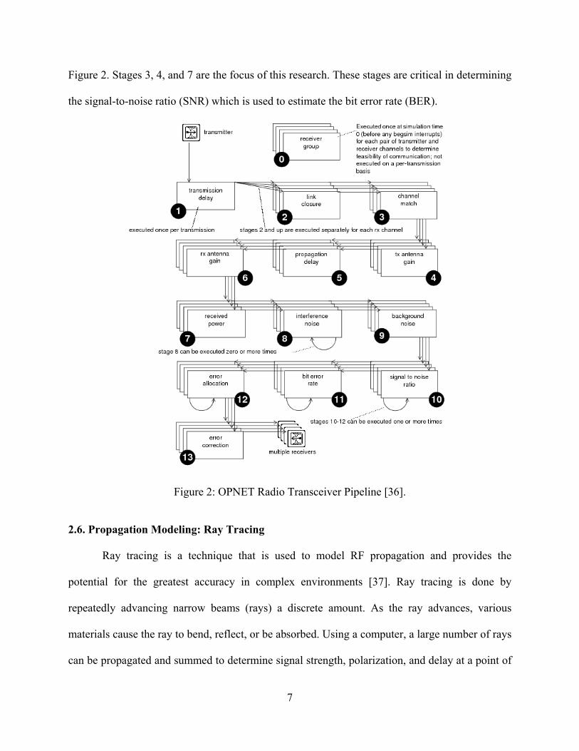
Figure 2. Stages 3, 4, and 7 are the focus of this research. These stages are critical in determining
the signal-to-noise ratio (SNR) which is used to estimate the bit error rate (BER).
Figure 2: OPNET Radio Transceiver Pipeline [36].
2.6. Propagation Modeling: Ray Tracing
Ray tracing is a technique that is used to model RF propagation and provides the
potential for the greatest accuracy in complex environments [37]. Ray tracing is done by
repeatedly advancing narrow beams (rays) a discrete amount. As the ray advances, various
materials cause the ray to bend, reflect, or be absorbed. Using a computer, a large number of rays
can be propagated and summed to determine signal strength, polarization, and delay at a point of

8
interest. For example, SAIC® Urbana™ wireless toolkit uses 3-D ray tracing to simulate
propagation and takes into account antenna radiation patterns, multipath, angle of arrival, delay,
etc. [38]. The two drawbacks to this technique are the large computational expense and the
requirement for an accurate 3-D representation of the region of interest. Furthermore, the
electromagnetic characteristics of the materials in the region must be specified.
2.7. Propagation Modeling: Statistical Models
Statistical models of RF propagation are based on both experimental and theoretical data.
They give a rough estimate of what the signal strength will be at a point of interest and are less
computationally expensive than the ray trace method. They are employed in network simulators
such as NS-2 and OPNET [11]; however, a majority of these models are not designed for
airborne wireless networks [39-41]. According to a study performed by Nadeel Ahmed et al.,the
two major contributors to link degradation in airborne networks are antenna orientation and
multipath due to ground reflections [42].
A practical model found in [41] yielded RSS values that were close to reality when
multipath due to ground reflection was present. To calculate the gain due to antenna orientation,
they modelled antenna radiation patterns using real-world data. They then used the common two-
ray model to determine RSS. This model is deterministic in nature. However, based on empirical
data, they added a Gaussian error to the output of the model to compensate for imperfections in
the hardware and the incomplete description of the wireless environment. This Gaussian error
had a standard deviation that was dependent on the mean RSS. They found that as the mean RSS
increased the standard deviation of the RSS decreased. By adding this error to their model, they
were able to estimate the precision of their simulation. Though their model was accurate for a
specific scenario, it does not accurately model airborne operations for two reasons. First, they

9
designed their model for strictly horizontal or vertical polarization, which for the airborne
environment is seldom reality. Second, their antenna model cannot accurately define complex
radiation patterns. To apply the two-ray model to airborne environment, the model must be
reformulated to handle all polarizations, and the antenna must be modeled to accurately account
for polarization and gain.
2.8. Antenna Modeling
Over the past 60 years, advancements in computational electromagnetics (CEM) have
increased the fidelity of antenna models; and, in the last decade, advancements in computer
technology have provided the computational power necessary to analyze these high fidelity
models. It is beyond the scope of this thesis to discuss all the advancements in CEM. Instead, the
model implemented in this research is discussed.
Like many engineering problems, antenna modeling can be framed in the frequency
domain. Solving Maxwell’s integral equations in the frequency-domain is the most popular and
widely used method for antenna design and analysis [43]. Two frequently used methods to solve
these equations in the frequency-domain are the finite element (FE) method and the Method of
Moments (MoM). The MoM is more efficient than the FE method when the antenna is
comprised solely of conducting material. Since the antenna used in the research was comprised
of only conducting material, the MoM was selected for this research. This method has improved
in capability and fidelity since the 1960s. Two common antenna problems simulated using the
MoM are wire and surface antennas. The latter is used in this research because it provides future
researchers the capability of analyzing more complex antenna structures.
In the simulation of a surface antenna, a surface integral equation is solved. Solving the
surface integral equation requires breaking the surface into smaller surface patches. Modeling the
10
antenna with surface patches was one of the more challenging aspects of modeling antennas
because expansion functions of the time did correctly model current continuity from patch-to-
patch [43]. In 1982, Rao, Wilton, and Glisson (RWG) developed the vector basis functions
which substantially improved the fidelity of the surface antenna simulation. Sergey N. Makarov,
whose code was adopted in this research, employed these vector basis functions and the MoM
[44]. For brevity and because many other resource are available for this type of antenna
modeling, further details of this model are not discussed in this thesis. Makarov’s codes can be
downloaded from [45].
2.9. Scalar, Vector, and Matrix Notations
Throughout the methodology and results section of this thesis, the following notations are
adhered to. Scalars are italicized. Vectors appear with an arrow on top (for example— and are
in column form. Matrices are bold and italicized.
2.10. Summary
This chapter discussed the background materials related to modeling an airborne RF
wireless communication system. Sections 2.2 and 2.3 discussed the growing demand for better
airborne communication systems. Section 2.4 discussed Major Durham’s work at AFIT using
OPNET to simulate an airborne wireless network, where he found that greater model fidelity was
needed to accurately model the physical layer. Section 2.5 briefly discussed network simulators
and the physical layer of the communication system. Sections 2.6 and 2.7 looked at how wireless
propagation could be modeled using ray tracing or statistical models. Ray tracing has the
potential for greater fidelity but is more computationally expensive and complex than statistical
model. Section 2.8 provided a background of the antenna modeling technique used in this
research. Section 2.9 defined the notation for scalars, vectors, and matrices in this thesis.

11
III Methodology
3.1. Chapter Overview
This chapter presents the development of a model for simulating the airborne wireless
environment. The model incorporates multipath due to ground reflects into the calculation of the
received signal strength (RSS). The more accurate this calculation is, the more realistic results
from flight path optimization and communication protocol development will be.
The method used in this research to characterize the wireless environment is the two-ray
model. This model takes into account the multipath due to ground reflection. Figure 3 shows the
two rays leaving the transmitting antenna and ending at the receiving antenna. In this model, the
effects of the airframe on the electromagnetic (EM) field are ignored.
Figure 3: Airborne Two-Ray Model.
The MATLAB® algorithm designed to implement the two-ray model splits the data flow
into two threads (Figure 4 and Figure 5). These two threads show the steps necessary to calculate
the EM field of the reflected and line-of-sight (LOS) rays. Each process block includes a

12
reference to the section that discusses the computation within that block. The outputs of these
two threads are combined for the calculation of the RSS at the receiving antenna.
Figure 4: Two-Ray Algorithm Flow Chart (Part 1 of 2).
13
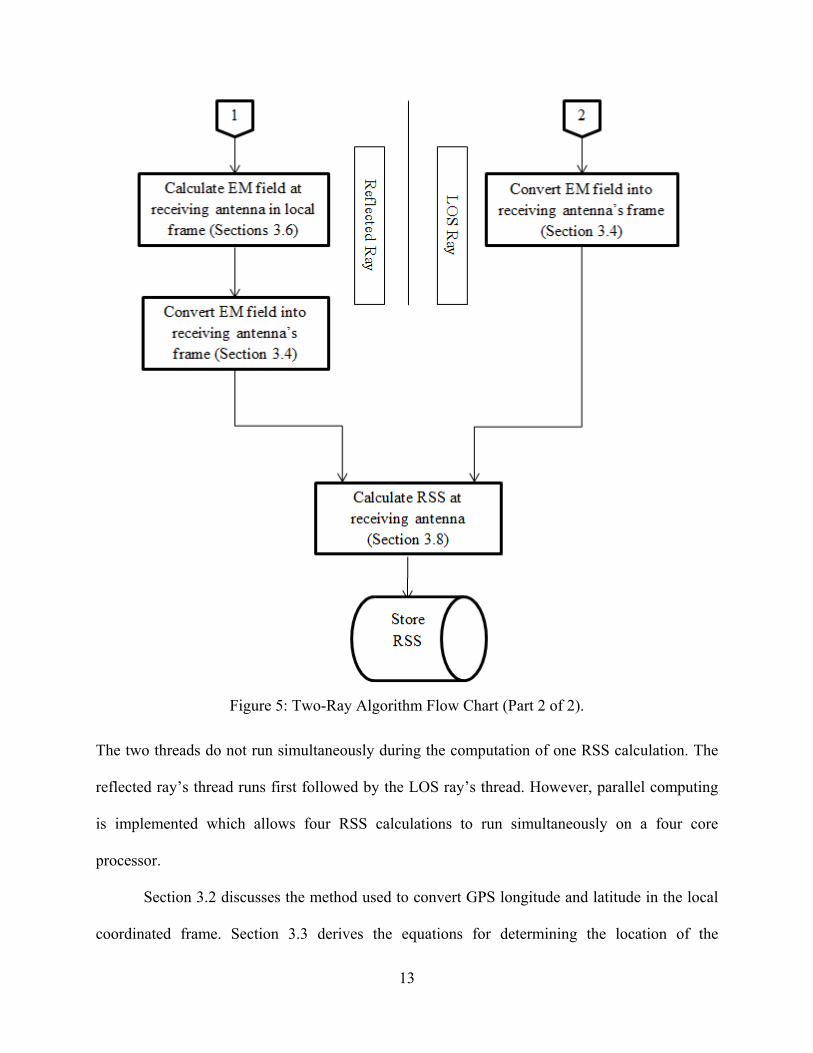
Figure 5: Two-Ray Algorithm Flow Chart (Part 2 of 2).
The two threads do not run simultaneously during the computation of one RSS calculation. The
reflected ray’s thread runs first followed by the LOS ray’s thread. However, parallel computing
is implemented which allows four RSS calculations to run simultaneously on a four core
processor.
Section 3.2 discusses the method used to convert GPS longitude and latitude in the local
coordinated frame. Section 3.3 derives the equations for determining the location of the

14
reflection point. Section 3.4 presents the transformation between local and antenna frames.
Section 3.5 discusses the method used to develop the antenna model and compares the simulated
radiation characteristics to the datasheet of the research antenna. Section 3.6 derives the
equations used to determine the strength and polarization of the reflected ray. Section 3.7 briefly
describes the method used to calculate the LOS ray at the receiving antenna. Section 3.8
discusses the method used to combine the two rays at the receiving antenna and the method used
to estimate the RSS. Section 3.9 describes the testing of the model in six validation scenarios.
Section 3.10 discusses the method used for performance evaluation of the model, and Section
3.11 summarizes the model developed in this chapter.
3.2. Conversion of Aircraft GPS Location into the Local Cartesian Frame
In the local frame, the ground is considered to be an infinite, flat plane with the origin
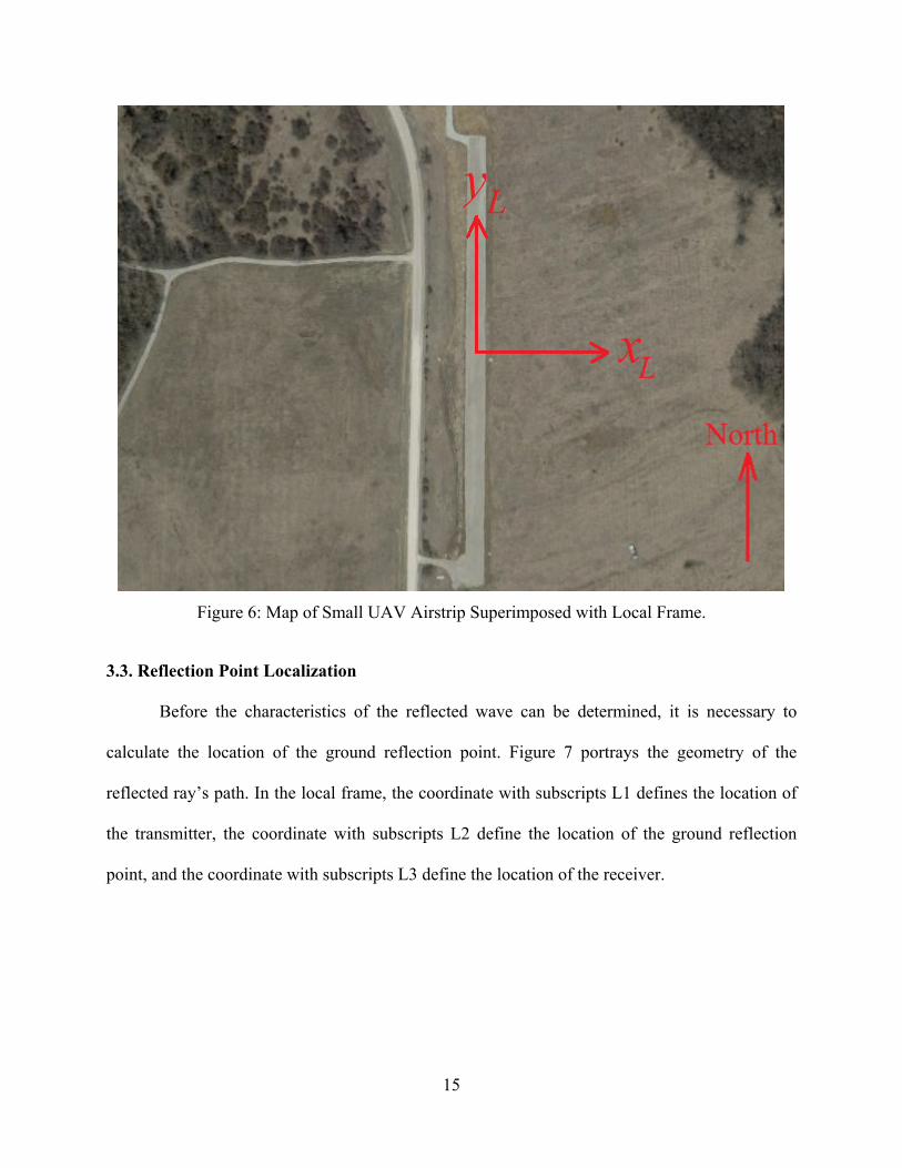
centered at longitude = -86.009389° and latitude = 39.34300°. This places the origin at the center
of the small UAV airstrip at Camp Atterbury, Johnson, Indiana (Figure 6). The flat plane model
is accurate for a small change in latitude and longitude. For this reason, the origin was placed at
the center of the runway. For the selected origin, a one-degree change in longitude results in an
86,206.576 m change in the + -axis direction, and a one-degree change in the latitude results in
an 111,022.01 m change in the + -axis direction [46]. The altitude stored by the autopilot is
equal to the displacement in the + -axis direction.
15
Figure 6: Map of Small UAV Airstrip Superimposed with Local Frame.
3.3. Reflection Point Localization
Before the characteristics of the reflected wave can be determined, it is necessary to
calculate the location of the ground reflection point. Figure 7 portrays the geometry of the
reflected ray’s path. In the local frame, the coordinate with subscripts L1 defines the location of
the transmitter, the coordinate with subscripts L2 define the location of the ground reflection
point, and the coordinate with subscripts L3 define the location of the receiver.

16
Figure 7: Reflection Geometry in Local Frame.
According to the law of reflection, the angle of incidence is equal to the angle of
reflection. This relationship is seen in Figure 7 with the angle α. The angle φ is calculated using
Equation 1:
cosφ (1)
The geometry is then viewed in two dimensions as shown in Figure 8, where is the
ground distance between the transmitter and the receiver and is calculated using Equation 2:
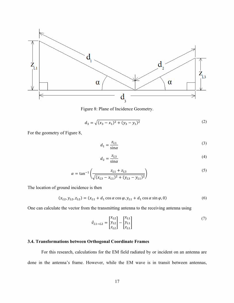
17
Figure 8: Plane of Incidence Geometry.
(2)
For the geometry of Figure 8,
sin (3)
sin (4)
tan (5)
The location of ground incidence is then
, , cos cos , cos sin , 0 (6)
One can calculate the vector from the transmitting antenna to the receiving antenna using
→ (7)
3.4. Transformations between Orthogonal Coordinate Frames
For this research, calculations for the EM field radiated by or incident on an antenna are
done in the antenna’s frame. However, while the EM wave is in transit between antennas,

18
calculations are done in the local frame or reflection frame. Therefore, a transformation between
orthogonal coordinate frames is necessary.
To transform the coordinates of a vector in the local frame into the antenna’s frame, four
direction cosine matrices (DCMs) which correspond to rotations in yaw, pitch, roll, and antenna
angle are developed. The rotations will align the -axis with the antenna and the -axis with
the left wing of the aircraft (Figure 9). Because the autopilot and GPS unit are located close to
the antenna, the origin of the reference frame used by the autopilot is assumed to be located at
the origin of the antenna’s frame.
Figure 9: Antenna's Coordinate Frame.
The first DCM, Equation 8, corresponds to a rotation about the about the yaw axis:
cos sin 0sin cos 00 0 1
(8)
Where γ is the yaw angle. A rotation is then performed about the pitch axis:
cos 0 sin0 1 0
sin 0 cos
(9)

19
Where β is the pitch angle. The third rotation is performed about the roll axis:
1 0 00 cos sin0 sin cos
(10)
Where δ is the roll angle. The final rotation is due to the position of the antenna with respect to
the aircraft (Appendix A). This rotation is about the y-axis by -5°:
cos 5° 0 sin 5°0 1 0
sin 5° 0 cos 5°
(11)
A vector is transformed from the local frame to the antenna frame by Equation 12:
(12)
Note that the matrix multiplication is not commutative and that the matrix multiplication must be
performed in the order prescribed by Equation 12.
To transform a vector from the antenna’s frame to the local frame, matrix algebra is used
to solve for in Equation 12. This yields
(13)
Since each of the frames is orthogonal, Equation 13 can be written as
(14)
Where is the transpose of .
3.5. Transmitting Antenna Model
In order to model the transmitting antenna, MATLAB codes written by Sergey N.
Makarov [44] were adopted. This code requires a 3-D model of the antenna created using
triangular patches. The antenna used for flight data collection was cut open to reveal the internal
geometry of the antenna (Figure 10).

20
Figure 10: Internal Geometry of Research Antenna.
Using the dimensions of the antenna, code was written that divided the antenna up into 15
sections, and these sections were populated with triangular patches (Figure 11). Each coil has 4
turns; and the feeding-edge, which is the location where the shielded cable connects to the
antenna, is located between the sections that have a 3.39-mm diameter and a 1.00-mm diameter.
Correspondingly, the feeding-edge is located at coordinate (0, 0, 0) in the MATLAB model.
Each section is modelled by a 2-D strip with a width equal to four times the radius of the wire for
that section [44, pp. 60].
Makarov’s code uses the 3-D model to calculate an impedance matrix. This matrix is
used in the determination of the electric current flowing on the antenna surface [44, pp. 3]. Once
the electric current flow is determined, the radiated field can be determined at any point in space.
Figure 12 shows a quantitative representation of the power passing through each triangular
subsection of a sphere with a radius of 100 m. The axes shown in Figure 12 correspond to the
axes of the antenna’s frame. The dark blue triangles represent the regions of lowest transmitted
power, and the dark red triangles represent the regions of highest transmitted power. A majority
of this antenna’s power is confined to low elevation angles, while the power remains
approximately constant for every azimuthal angle. This pattern is common for omni-directional
antennas, and the antenna used in this research is omni-directional [47].

21
Figure 11: 3-D Antenna Model made from 2-D Patches.

22
Figure 12: Qualitative Representation of Power Distribution.
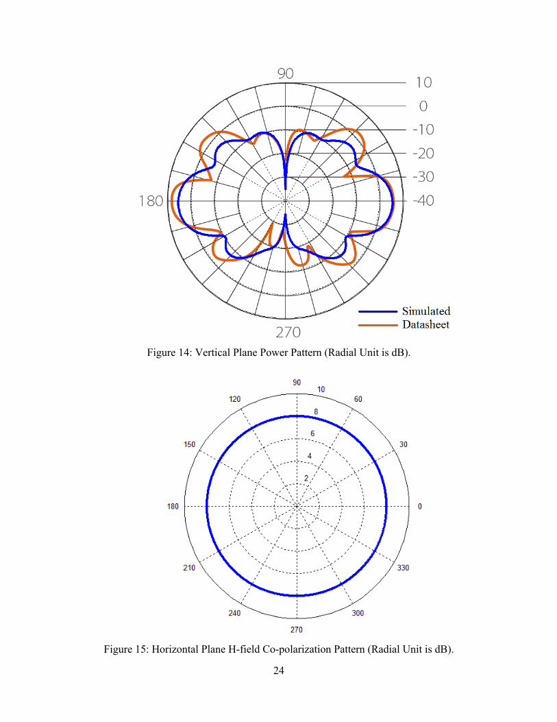
In order to validate the accuracy of this model, the radiation patterns must be compared to
the antenna’s datasheet. Figure 13 shows the datasheet’s vertical plane co-polarization pattern in
orange. The vertical plane co-polarization E-field pattern generated by the simulation is
superimposed in blue.

23
Figure 13: Vertical Plane Co-polarization E-field Pattern (Radial Unit is dB).
Figure 12 shows the comparison of the datasheet’s vertical plane co-polarization pattern
to the pattern representing the simulated transmitted power at a given elevation. This figure looks
more like the pattern seen in the datasheet than Figure 13. The datasheet’s vertical plane co-
polarization pattern is asymmetric. This asymmetry may be a result of the test configuration or, if
simulation was employed, the model used to simulate the antenna’s radiation. The simulated
pattern in blue has negligible asymmetry. Figure 15 shows the horizontal plane H-field co-
polarization pattern. This pattern is the same as the horizontal plane co-polarization pattern in the
datasheet.
The simulated antenna model produced similar propagation patterns to those found in the
datasheet; consequently, this model was used in all simulations. Furthermore, the 3-D patch
model was used to compute both the radiated field of the transmitting antenna and the current in
the receiving antenna.
24
Figure 14: Vertical Plane Power Pattern (Radial Unit is dB).
Figure 15: Horizontal Plane H-field Co-polarization Pattern (Radial Unit is dB).

25
3.6. Reflection Modelling
Reflections are normally modeled in the plane of incidence, which is the plane containing
the incident, reflected, and transmitted rays (Figure 8). Many electromagnetics and wireless
communications textbooks characterize the interaction taking place on the reflecting surface for
both parallel and perpendicular polarizations [39, 48-51]. For this model, the rays are assumed to
be travelling through free space and reflecting from the soil. It is also assumed that the receiving
antenna and reflection point are in the far-field. In the far-field, and are related by
Η (15)
1E
(16)
where is the intrinsic impedance, is the electric field (E-field) vector, is the magnetic field
(H-field) vector, is the vector from the transmitting antenna to the point of interest, and r is the
magnitude of . Equations 15 and 16 are good approximations when
2
(17)
where L is the maximum dimension of the antenna and is the wavelength of the
electromagnetic wave in free space [44, pp. 44]. At 2.4 GHz and with an antenna length of 28.5
cm, (2 / ) = 1.30 m. For all of the flight tests, r > 1.30 m, which justifies the use of the far-
field approximation in this research.
Because the E-field and H-field are related, only the E-field is considered in the reflection
equations. At the point of reflection, the incident E-field in the antenna’s frame, , can be
calculated using the antenna model. The E-field components in the antenna frame are then
converted to the local frame using DCMs. However, the local frame may not align with the
parallel and perpendicular polarization vectors, and respectively. Because the equations
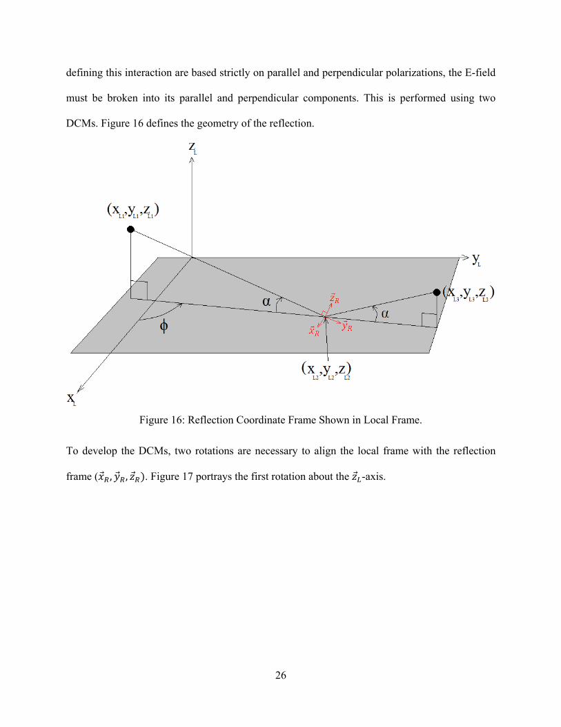
26
defining this interaction are based strictly on parallel and perpendicular polarizations, the E-field
must be broken into its parallel and perpendicular components. This is performed using two
DCMs. Figure 16 defines the geometry of the reflection.
Figure 16: Reflection Coordinate Frame Shown in Local Frame.
To develop the DCMs, two rotations are necessary to align the local frame with the reflection
frame ( , , . Figure 17 portrays the first rotation about the -axis.

27
Figure 17: View from above xy-plane.
Using the φ calculated in Section 3.3, the amount of rotation about the -axis required to align
with is -(90°- φ). The DCM used for this rotation is
cos 90° sin 90° 0sin 90° cos 90° 0
0 0 1
(18)
The second rotation is shown in Figure 18. This rotation is about the axis by –α. The
corresponding DCM is
1 0 00 cos α sin0 sin cos
(19)

28
Figure 18: Plane of Incidence View.
The multiplication of these DCMs with the incidence E-field, , yields
(20)
Where is the incidence E-field in the reflection frame. Once the incidence E-field is in the
reflection frame, the depolarization matrix is used to calculate the strength and polarization of
the reflected E-field in the reflection frame [39, pp. 117]. This matrix is given by
Γ 0 00 0 00 0 Γ∥
(21)
Where Γ∥ and Γ are the parallel and perpendicular reflection coefficients respectively, and
Γ∥sin sinsin sin
(22)
Γsin sinsin sin
(23)
Where , is the intrinsic impedance and is given by
, , ,⁄ (24)

29
where is the permeability of free space which equals 4 10 H/m; is the permittivity of
free space which equals 8.854 10 F/m; is the permeability of the soil and is normally
equal to the permeability of free space [52]; and is the permittivity of the soil and for
simplicity equal to 3.4 [51, pp. 35]. This simplification is made because ground samples at
the flight area were not analyzed and the added complexity of having a complex (real and
imaginary parts) may not add substantial accuracy to the solution. This simplified case is known
as lossless reflection. Before equations 22 and 23 can be used, the transmission angle, , must
be solved using Snell’s Law:
90° sin sin 90°
(25)
The reflected field in the reflection frame, ,is given by
(26)
The next step is to compute the reflected field in the local frame. Parallel component of
the reflected field does not coincide with the reflection frame’s . To align the local frame with
the perpendicular and parallel components of the reflected field, the first rotation is the same, but
the second rotation is about the axis by +α. This results in the following DCM:
1 0 00 cos α sin0 sin cos
(27)
The equation to compute the reflected E-field in the local frame from the incidence E-
field in the local frame is given by
(28)
30
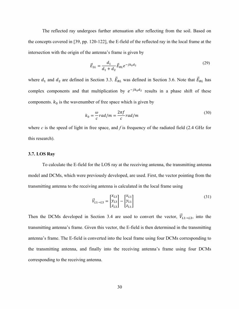
The reflected ray undergoes further attenuation after reflecting from the soil. Based on
the concepts covered in [39, pp. 120-122], the E-field of the reflected ray in the local frame at the
intersection with the origin of the antenna’s frame is given by
(29)
where and are defined in Section 3.3. was defined in Section 3.6. Note that has
complex components and that multiplication by results in a phase shift of these
components. is the wavenumber of free space which is given by
/2
/ (30)
where c is the speed of light in free space, and f is frequency of the radiated field (2.4 GHz for
this research).
3.7. LOS Ray
To calculate the E-field for the LOS ray at the receiving antenna, the transmitting antenna
model and DCMs, which were previously developed, are used. First, the vector pointing from the
transmitting antenna to the receiving antenna is calculated in the local frame using
→ (31)
Then the DCMs developed in Section 3.4 are used to convert the vector, → , into the
transmitting antenna’s frame. Given this vector, the E-field is then determined in the transmitting
antenna’s frame. The E-field is converted into the local frame using four DCMs corresponding to
the transmitting antenna, and finally into the receiving antenna’s frame using four DCMs
corresponding to the receiving antenna.

31
3.8. Receiving Antenna Model
To compute the received power, the 3-D patch model developed in Section 3.5 is again
used. In the case of receiving antenna, the radiated field incidence on the antenna’s surface will
induce current flow in the antenna. Code was developed by Makarov in [44] to handle the
incidence of a single plane wave on the surface of an antenna; however, the two-ray model
requires the superposition of two plane waves on the antenna surface. The far-field
approximation is again used.
The E-field of the LOS ray and reflected ray in the local frame at the intersection with the
origin of the antenna’s frame are and respectively. These E-fields are transformed into the
receiving antenna’s frame using the DCMs developed in Section 3.4. In the antenna frame, the
two rays intersect at the origin of the frame and consequently at the feeding point of the antenna.
In the far-field, these rays are approximated using uniform plane waves. Figure 19 shows the
incidence of a single plane wave on an antenna. This plane wave changes in both phase and
amplitude along the antenna. Since the dimensions of the antenna are small, the changes in
amplitude are negligible; however, the change in phase is not negligible and is computed using
the distance, d, the wave front moves in the direction of . The wave vector, , is pointed in the
same direction as the ray and has a magnitude of for Section 3.6. The distance, d, is the
projection of onto which is the unit vector in the direction of . Multiplying by d gives the
amount of phase shift in radians. Using complex numbers, the E-field at each point along the
antenna produced by a single ray is
∙ (32)
Where is the E-field at the origin, and (·) denotes the dot product. This approach was used by
Makarov and is described in [53].

32
Figure 19: Incidence Model Geometry.
Since two waves are arriving at the antenna, the E-field created by each wave front is first
computed and then added together at each patch along the antenna. The current in the antenna is
then calculated using Makarov’s code, and the received power is estimated using the current
through the feed-point and the real part of the antenna’s impedance. The received power is given
by
12
(33)
Where Z is the complex impedance of the antenna (which is 227.73+j9.6215 Ω from simulation),
and I is the amplitude of the steady-state alternating current. Note that the real part of the
impedance which was calculated using the 3-D patch model is higher than the datasheet specified
(50 Ω) [47]. This is due to imperfections in the modeling of the antenna.

33
3.9. Validation Testing
In order to ensure that the algorithm was working properly, several tests were performed
in simulation. The first, three tests were done at high altitude (10 km) to ensure both the
transmitting and receiving antenna models were working correctly. In the first test, the
transmitting and receiving aircraft were positioned at local coordinate positions (0, 0, 10000) m
and (0, 100, 10000) m respectively. Both aircraft were pointed in the x-axis direction. The
transmitting plane performed a rotation about the roll axis (Figure 20). Figure 21 is RSS pattern
generated as the transmitting aircraft rotates. This is identical to Figure 14 and proves that the
transmitting antenna model is working properly. The plot is offset by 80.6774 dB to prohibit
negative dB values, which causes trouble when using the MATLAB polar function.
Figure 20: Test Setup 1 for Vertical Plane Power Pattern Analysis.

34
Figure 21: Validation Vertical Plane Power Pattern.
Similarly the receiving aircraft was rotated (Figure 22), and the pattern seen in Figure 21
was again repeated. This repetition follows in accordance with the reciprocity theorem [54, pp.
147-150] and proves that the receiving antenna model was functioning properly.
Figure 22: Test Setup 2 for Vertical Plane Power Pattern Analysis.
The third test looked at polarization mismatch. The transmitting and receiving aircraft
were positioned at local coordinate positions (0, 0, 10000) m and (100, 0, 10000) m respectively.

35
Both aircraft were pointed in the x-axis direction. The receiving plane was rotated about the roll
axis to create a polarization mismatch (Figure 23).
Figure 23: Test Setup for Polarization Mismatch Analysis.
According to [54, pp. 76], the polarization loss factor for linear polarization is given by
|cos | (34)
where the angle is defined in Figure 23 above. For comparison of the simulated RSS to the
theoretical RSS, the theoretical RSS is given by
10log |cos | max (35)
where is the received signal strength in dB that is computed from the simulation, and
is the value added to the RSS value to avoid plotting of negative radii in the polar plot.
In addition, values which fall below zero, which takes place when goes to 90° or -90°,
are reset to zero. This prevents from going towards negative infinity. In Figure 24, the
simulated RSS is shown in blue, and the RSS computed from Equation 35 is shown in red. The
red and blue curves show significant overlap proving that the simulation model is functioning
properly. The curves do not overlap at every angle because the antenna is not perfectly linearly
polarized.

36
Figure 24: Simulated and Theoretical RSS vs. Polarization Mismatch Angle.
The final three tests are performed at 1.50-m altitude with the transmitting aircraft at the
coordinate (0, 0, 1.50) m. This ensures that the effects of ground reflection will be observable in
the RSS solution. For the first test, both antennas are perpendicular to the ground plane, and the
receiving aircraft is moved along the y-axis direction from (0, 0, 1.50) m to (0, 70, 1.50) m.
Figure 25 shows the simulated RSS value in blue, and the RSS value predicted by the Friis
equation [44, pp. 81] is shown in green. The Friis equation is given by
4
(36)

37
where is the transmitted power in watts; is the linear gain of the transmitting antenna;
is the linear gain of the receiving antenna; is the wavelength of the electromagnetic wave; and r
is the distance between the antennas.
Equation 36 in dB is given by
10log 20log 4 20log (37)
Only the last term on the right side of Equation 37 varies with distance. The rest of the terms
remain constant. Therefore, Equation 37 can be written as
20log (38)
Where C is a constant. At a distance of one meter, the last term of Equation 38 cancels out, and
the constant C can be solved for. In Figure 25, the simulated RSS is above and below the Friis
value due to constructive and destructive interference created by the ground reflection. This
proves that the algorithm is combining both the LOS and reflected rays for vertically oriented
antennas.

38
Figure 25: RSS vs. Distance (Height = 1.50 m and Vertical Polarization).
The second test was similar to the previous test. However, this time the antennas were
oriented parallel to the ground plane and one another with the direction of highest gain pointed
towards each other. Figure 26 again shows the effects of constructive and destructive
interference and resembles [41, Fig. 6(c)] which was computed for the same antenna height and
orientation using a different method. This proves that the algorithm is properly combining both
the LOS and reflected rays for antennas oriented parallel to the ground plane.

39
Figure 26: RSS vs. Distance (Height = 1.50 m and Horizontal Polarization).
In the final test, both antennas were placed vertically with respect to the ground plane,
and the transmitting antenna was again placed at (0, 0, 1.5) m. The receiving antenna was moved
to 40,000 positions in x- and y-axes directions while maintaining a height of 1.5 m above ground
level. This produced the interference pattern seen in Figure 27 and proved that the algorithm is
combining the two rays in the same manner in all directions.

40
Figure 27: RSS Pattern Produced by Interference (Height = 1.50 m and V-Pol.).
3.10. Performance Evaluation
To evaluate the performance of the model, the results section compares the two-ray
model to the data attained from flight-testing. In addition, this section evaluates a one-ray model
using only the LOS ray. This model is a simplification of the two-ray model where the reflected
ray is removed from the calculation of E-field at the receiving antenna. Furthermore, this section
also evaluates the Friis model (Equation 38) and compares it to the other models. To rate the
performance of the models, the results section displays the error between the simulated RSS and

41
measured RSS and shows the bias and standard deviation of the error with respect to the distance
between antennas. A bias of zero means that the model is accurate and on average will produce
the right result. A lower standard deviation means the model has greater precision. Note the
precision and accuracy of the flight data affects the precision with which the simulated results
can match the measured results. If errors are present in the measurement of location and attitude,
the output of model will also have errors.
Before evaluation, all the models require calibration. The algorithm sets the input to the
one-ray and two-ray models to a 10 V amplitude sinusoid. By varying the voltage amplitude the
model can be calibrated; however, adding a constant value to the simulated RSS is much faster
and produces the same result. The calibrated RSS equation is given by
20log (39)
Where is the simulated RSS in watts, and E is a constant that is chosen to reduce the bias of
the error between simulated RSS and measured RSS. Similarly, C in Equation 38 is also chosen
to reduce the bias of the error for the Friis model.
3.11. Summary
This chapter presented the two-ray model that simulates the airborne wireless
environment. To determine the radiation characteristics of the transmitting antenna, MATLAB
codes developed by Sergey N. Makarov were used to analyze a 3-D model of the research
antenna made from 2-D triangular patches. DCMs were developed to transform vectors between
coordinate frames, and a lossless reflection model was developed to determine the strength and
polarity of the reflected ray. To determine the power generated at the receiving antenna, codes
written by Makarov and the 3-D model developed in this chapter were again utilized. This model
was tested and performed as anticipated showing the effects of polarization, directional gain, and

42
interference. Lastly, statistical evaluation of the error between the simulated RSS and measured
RSS was proposed as the method for evaluating the performance of the one-ray, two-ray, and
Friis models.

43
IV Analysis and Results
4.1. Chapter Overview
This chapter compares the one-ray, two-ray, and Friis model results against data collected
from several flight test. In all sections, the data is analyzed when the required aircraft is/are in
flight. Section 4.2 discusses the yaw angle correction applied to the flight data. Section 4.3
evaluates the performances of the models in the air-to-air (AtoA) scenario and provides the
calibrated equations for the models. Sections 4.4 and 4.5 analyze the ground-to-air (GtoA) and
air-to-ground (AtoG) scenarios and identify key features of the results. Section 4.6 combines the
data from all scenarios and provides a more in depth statistical analysis. Section 4.7 summarizes
the results found in this chapter.
4.2. Yaw Angle Correction
In Sections 4.2-4.4, the flight data is analyzed using both the yaw angle provided by the
autopilot and the yaw calculated from the direction of the vector between consecutive GPS
locations. Early in the analysis, it was found that the yaw angle provided by the autopilot was
unreliable before the aircraft was in flight. The yaw angle drifted while the aircraft was
stationary on the ground (Figure 83 in Appendix E). Even during flight, the yaw angle
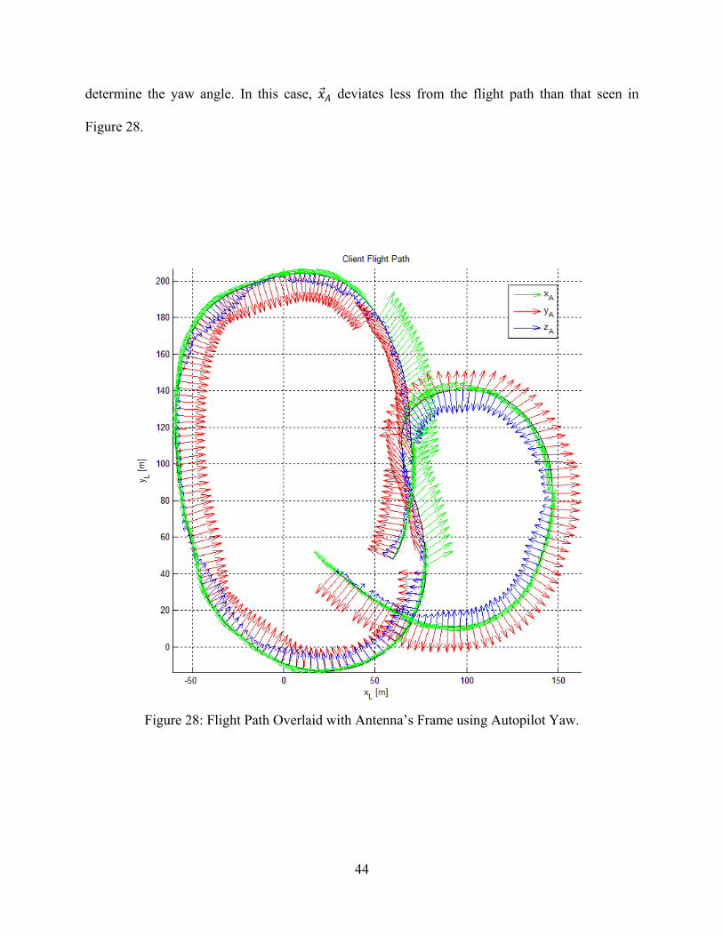
sometimes points in a direction off the flight path. This is observed in Figure 28, where the
arrows shown are in the directions of the axes of the antenna’s frame as defined in Section 3.4.
The deviation of from the flight path could be due to the high winds experienced the day of
flight-testing. However, the locations at which these deviations occur and direction of at these
locations led to the conclusion that the heading solution of the autopilot was inaccurate. This
could be due to the ArduPlane program or the inaccuracies associated with the magnetometer.
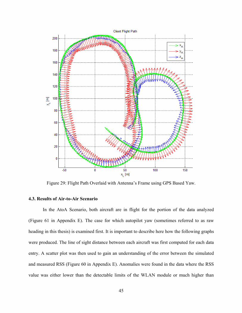
Figure 29 shows the flight path overlaid with the antenna’s frame and using GPS positions to
44
determine the yaw angle. In this case, deviates less from the flight path than that seen in
Figure 28.
Figure 28: Flight Path Overlaid with Antenna’s Frame using Autopilot Yaw.
45
Figure 29: Flight Path Overlaid with Antenna’s Frame using GPS Based Yaw.
4.3. Results of Air-to-Air Scenario
In the AtoA Scenario, both aircraft are in flight for the portion of the data analyzed
(Figure 61 in Appendix E). The case for which autopilot yaw (sometimes referred to as raw
heading in this thesis) is examined first. It is important to describe here how the following graphs
were produced. The line of sight distance between each aircraft was first computed for each data
entry. A scatter plot was then used to gain an understanding of the error between the simulated
and measured RSS (Figure 60 in Appendix E). Anomalies were found in the data where the RSS
value was either lower than the detectable limits of the WLAN module or much higher than

46
anticipated. For this reason, threshold lines were drawn using Equations 40 and 41, and data
points outside the threshold lines were ignored.
2035
(40)
2035
(41)
Where distance is the LOS distance between the antennas. Figure 30 shows the results of the
statistical analysis on the data found in the scatter plot (Figure 60 in Appendix E). In Figure 30,
30, 31, and 32, the error is examined for every 20-m section of distance (0-20 m, 20-40 m, and so
on), the bias and standard deviation are graphed at the midpoint of each section. The histogram
shows the number of data points recorded within each 20-m section. These figures show the
relationship between error and distance.
The Friis equation was calibrated to drive the bias at 250 m to zero and is given by
36.638 20log (42)
Where r is the distance between the antennas. The one-ray and two-ray models were also
calibrated at 250 m to reduce the error bias to zero, and Equation 43 is used by both:
33.5 20log (43)
Where is the simulated RSS in watts. These equations are used in the remaining analysis.
Since the wireless module will only report RSS for the last received packet, values that fall
below -92 dBm (the lowest value the wireless module can measure) are set equal to -92 dBm.
Figure 30 shows a tendency of the Friis equation to estimate above the measured RSS value at
distances under 150 m. This tendency is due in part to the Friis equation not taking into account
the variations in antenna gain due to polarization and propagation direction.

47
Figure 30: Statistical Analysis of AtoA Scenario with Raw Heading.
48
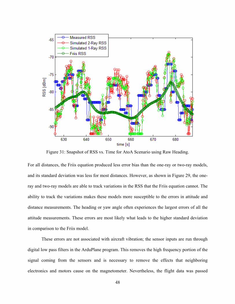
Figure 31: Snapshot of RSS vs. Time for AtoA Scenario using Raw Heading.
For all distances, the Friis equation produced less error bias than the one-ray or two-ray models,
and its standard deviation was less for most distances. However, as shown in Figure 29, the one-
ray and two-ray models are able to track variations in the RSS that the Friis equation cannot. The
ability to track the variations makes these models more susceptible to the errors in attitude and
distance measurements. The heading or yaw angle often experiences the largest errors of all the
attitude measurements. These errors are most likely what leads to the higher standard deviation
in comparison to the Friis model.
These errors are not associated with aircraft vibration; the sensor inputs are run through
digital low pass filters in the ArduPlane program. This removes the high frequency portion of the
signal coming from the sensors and is necessary to remove the effects that neighboring
electronics and motors cause on the magnetometer. Nevertheless, the flight data was passed

49
through a first-order low-pass 1 Hz filter, but this method showed no improvement over using
the raw data from the autopilot.
The AtoA flight was again analyzed with the autopilot yaw angle replace with a GPS
based heading. For this case, the standard deviation of the error for the one-ray and two-ray
models was reduced for a majority of the distances; the bias however was better at some distance
and worse at others (Figure 65 in Appendix E).
4.4. Results of Ground-to-Air Scenario
For the GtoA Scenario, the aircraft containing the access point remained stationary on the
ground while the aircraft containing the client was flown. Figure 32 shows that for a majority of
the data entries the distance between the antennas was less than 200 m. For a majority of the
distances, the one-ray and two-ray models have less error bias than the Friis model. For distances
that have more than fifty data entries, the standard deviation of error for the one-ray and two-
models varies by approximately one dBm above and below that of the Friis model. The use of a
GPS based heading does not appear to perform any better (Figure 78 in Appendix E).

50
Figure 32: Statistical Analysis of GtoA Scenario with Raw Heading.

51
4.5. Results of Air-to-Ground Scenario
For the AtoG Scenario, the aircraft containing the client remained stationary on the
ground while the aircraft containing the access point was flown. Figure 33 shows a majority of
the data entries are around a 170-m separation distance between antennas. In this case, the error
bias for the Friis model is again higher in magnitude than the one-ray or two-ray models for
distances less than 270 m. For a majority of the distances, the standard deviation for the Friis
model error is less than that for the one-ray or two-ray. The use of a GPS based heading does not
appear to perform any better (Figure 91 in Appendix E).
Figure 33: Statistical Analysis of AtoG Scenario with Raw Heading.

52
4.6. Combined Result of All Scenarios
Due to the limited data set available for each scenario, the flight data from all 3 scenarios
were combined, and the results are shown in Figure 34.
Figure 34: Statistical Analysis of All Scenarios with Raw Heading.
For a majority of the distances, the error bias of one-ray and two-ray is less than the error bias of
the Friis model. The exception is at distances greater than 330 m where the number of data
53
entries is less than 400 per 20-m section. The standard deviation of the error for the one-ray and
two-ray models is greater for a majority of the distances than the Friis model.
As stated earlier, the tendency of the Friis equation to estimate above the measured RSS
value is due in part to the Friis equation not taking into account the variations in antenna gain
due to polarization and propagation direction. To prove that this is indeed true, the elevation
angle is first defined, and then the error is evaluated with respect to the elevation angle between
the aircraft.
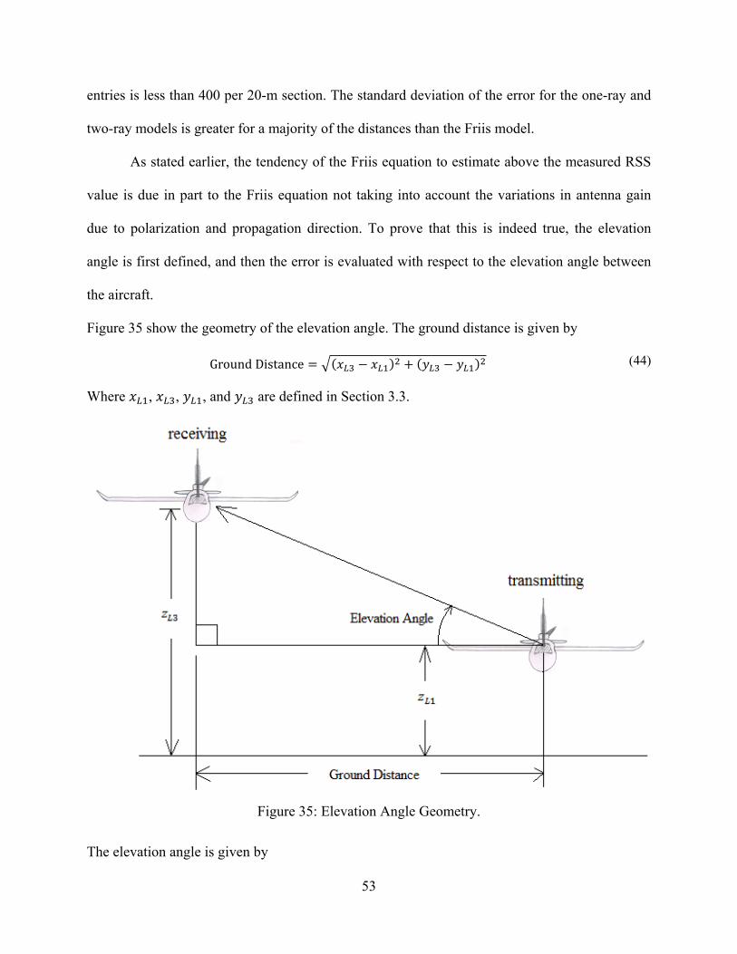
Figure 35 show the geometry of the elevation angle. The ground distance is given by
GroundDistance (44)
Where , , , and are defined in Section 3.3.
Figure 35: Elevation Angle Geometry.
The elevation angle is given by

54
ElevationAngle tan (44)
Where and are defined in Section 3.3. Using the definition of the elevation angle, the bias
and standard deviation of the error between the simulated and measured results were plotted in
Figure 36. This plot shows that as the elevation angle moves from zero the Friis error begins to
have a positive bias. Furthermore, it shows that the one-ray and two-ray experience a negative
bias as the elevation angle moves from zero. This bias is due to inaccuracies in the antenna
model. Figure 14 of Section 3.5 reveals that the lobes above and below the main horizontal lobes
are smaller than the datasheet specifies, and this causes the negative bias seen in Figure 36.
Figure 36 shows how the error is related to the elevation angle, but it does not prove why
the error bias of the Friis model increased as the distance between the antennas decreased. To
prove this the elevation angle with respect to the distance between the antennas must be plotted.
The elevation angle however has both positive and negative values. This leads to cancellation
and predicts a mean elevation angle closer to zero. For sake of evaluation, if it is assumed that
Figure 36 is symmetric across the vertical axis (which is not far from reality), then we need only
look at the absolute value of the elevation angle. Figure 37 reveals that the mean of the absolute
value of the elevation angle is increasing as distance decreases. This increase in elevation angle
causes increasing, positive bias in the error of the Friis model and decreasing, negative bias in
error for the one-ray and two-ray models. These results prove why the error bias of the Friis
model increased as the distance between the antennas decreased and why the bias of the one-ray
and two-ray models became more negative as the distance between the antennas decreased.

55
Figure 36: Error Statistics of All Scenarios with respect to Elevation Angle.

56
Figure 37: Bias of Errors and Mean Absolute Value of Elevation Angle vs. Distance
4.7. Summary
For the combination of all scenarios, the one-ray and two-ray models had a lower error
bias than the Friis model for a majority of the antenna separation distances. This means that on
average the one-ray and two-ray models produced the correct RSS value. On the other hand, the
Friis model at short distances on average produced RSS values that were higher than the

57
measured values, which was linked to the Friis equation not taking into account the variations in
antenna gain due to polarization and propagation direction. In addition, the negative error bias of
the one-ray and two-ray models at short distances was linked to inaccuracies in the modelling of
the antenna. The standard deviations of the errors for the one-ray and two-ray models were larger
than that of the Friis model because of inaccuracies in the antenna model and the measurements
of location and attitude. Lastly, the two-ray model performed almost identical to the one-ray
model and showed no signs of improved accuracy or precision.

58
V Conclusions and Recommendations
5.1. Chapter Overview
This chapter concludes the research and presents recommendations for future research.
Section 5.2 discusses the justification for this research. Section 5.3 discusses the goals of this
research. Section 5.4 describes the contribution of this research to flight path planning, antenna
selection, and protocol simulation. Section 5.5 provides a summary of the research findings.
Section 5.6 describes the significance of this research, and Section 5.7 provides
recommendations for future research.
5.2. Justification for Research
The reason for doing this research was to increase the fidelity of airborne wireless
networking simulations. By doing so, the aircraft flight paths can be better optimized, and
routing protocols can be tested in a simulation environment closer to reality. Static wireless
network planning will also benefit from higher fidelity.
5.3. Research Goals
This research had three goals. The first goal was to develop a method and algorithm for
modeling wireless communication in a simplified, rural, outdoor environment. This model used
the position and attitude of each aircraft to predict the RSS. This model took into account
polarization and multipath interference due to ground reflection. The second goal was to devise a
system to acquire flight telemetry and RSS measurements. The system is discussed in detail in
the appendices. The final goal was to validate the model by comparison with measured flight
data.

59
5.4. Research Contribution
This research developed a model of the physical layer of an airborne communication
system. This model was tested with real-world flight data collected using a system developed in
this research. This model can be used in the optimization of flight paths to maintain the greatest
signal strength. It can also be used in the selection and development of antennas for use in a
specific airborne scenario. With modifications, it can simulate radio direction finding via phase
shift analysis. Lastly, it provides a foundation for network simulation. This model can be
extended to encompass the higher layers of the Open System Interconnection (OSI) model [11].
Employing this model in the physical layer provides for higher fidelity than that seen in many
network simulators which do not incorporate computational electromagnetics (CEM) for antenna
modeling.
5.5. Conclusions of Research
The two-ray model, on average, produced the correct result at all distances and was more
accurate than the Friis model for the combination of all flight test scenarios. It was not however
more accurate than the one-ray model. Inaccuracy in the antenna model caused the simulated
results from the one-ray and two-ray models to be lower than the measured RSS at elevation
angles above 20° and below -20°. Contrarily the results from the Friis model were higher than
the measured RSS at elevation angles above 20° and below -20°. The standard deviation of the
one-ray and two-ray models was also higher due to both inaccuracies in the model and errors in
the measurement of the location and attitude. Figure 25 of Section 3.9 shows that small errors in
the measurement of location can result in large variations of the predicted signal strength.
Because the one-ray model is simpler and had the same accuracy as the two-ray model, it is the
best model to use for the data collected in this research.
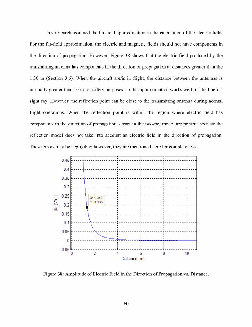
60
This research assumed the far-field approximation in the calculation of the electric field.
For the far-field approximation, the electric and magnetic fields should not have components in
the direction of propagation. However, Figure 38 shows that the electric field produced by the
transmitting antenna has components in the direction of propagation at distances greater than the
1.30 m (Section 3.6). When the aircraft are/is in flight, the distance between the antennas is
normally greater than 10 m for safety purposes, so this approximation works well for the line-of-
sight ray. However, the reflection point can be close to the transmitting antenna during normal
flight operations. When the reflection point is within the region where electric field has
components in the direction of propagation, errors in the two-ray model are present because the
reflection model does not take into account an electric field in the direction of propagation.
These errors may be negligible; however, they are mentioned here for completeness.
Figure 38: Amplitude of Electric Field in the Direction of Propagation vs. Distance.
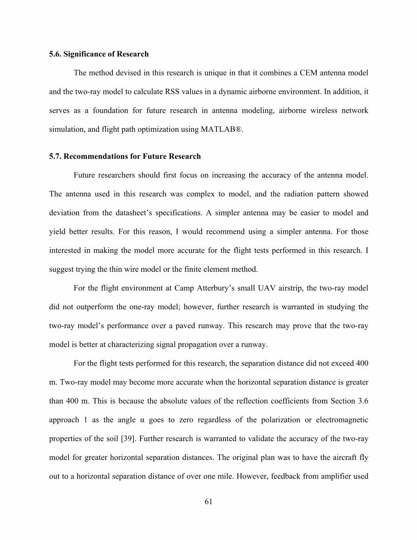
61
5.6. Significance of Research
The method devised in this research is unique in that it combines a CEM antenna model
and the two-ray model to calculate RSS values in a dynamic airborne environment. In addition, it
serves as a foundation for future research in antenna modeling, airborne wireless network
simulation, and flight path optimization using MATLAB®.
5.7. Recommendations for Future Research
Future researchers should first focus on increasing the accuracy of the antenna model.
The antenna used in this research was complex to model, and the radiation pattern showed
deviation from the datasheet’s specifications. A simpler antenna may be easier to model and
yield better results. For this reason, I would recommend using a simpler antenna. For those
interested in making the model more accurate for the flight tests performed in this research. I
suggest trying the thin wire model or the finite element method.
For the flight environment at Camp Atterbury’s small UAV airstrip, the two-ray model
did not outperform the one-ray model; however, further research is warranted in studying the
two-ray model’s performance over a paved runway. This research may prove that the two-ray
model is better at characterizing signal propagation over a runway.
For the flight tests performed for this research, the separation distance did not exceed 400
m. Two-ray model may become more accurate when the horizontal separation distance is greater
than 400 m. This is because the absolute values of the reflection coefficients from Section 3.6
approach 1 as the angle α goes to zero regardless of the polarization or electromagnetic
properties of the soil [39]. Further research is warranted to validate the accuracy of the two-ray
model for greater horizontal separation distances. The original plan was to have the aircraft fly
out to a horizontal separation distance of over one mile. However, feedback from amplifier used

62
to boost the RF signal of the WLAN modules caused the modules to fail (Appendix A). The
modules functioned for several hours before failing and may have failed due to thermal issues.
This research used WLAN modules in order to make RSS measurements. In order to gain
a better understanding of the physical layer, a software defined radio should be used. A software
defined radio opens the possibility of testing different modulation schemes and operating at a
variety of frequencies. In addition, software defined radios could be used to perform RF source
localization and navigation via signals of opportunity. Future researches should study how to
implement these radios on a small unmanned aerial vehicle.
In February of 2014, Steve Perlman announced the development of technology called
pCell [55]. This technology relies on deliberate interference of electromagnetic signals, which is
in opposition to previous communication technology. Each pCell radio transmits part of the
signal to be picked up by the receiver. Through precise timing, the signals combine at one point
in space to provide the full signal. This system has been lab tested and has shown drastic
improvement in bandwidth over legacy systems. If this system can be employed airborne
environment, it could provide a means for a more efficient and reliable communications. Future
researchers should look into the implementation of this technology into future communication
systems.

63
Appendix A. Hardware Configuration
The data collection portion of this research was performed using two aircraft. The first
aircraft contained a WLAN module which was configured as an access point, while the second
aircraft contained a WLAN module which was configured as a client. The second aircraft was
used to take measurements of the received signal strength (RSS). Though the ArduPilot Mega
(APM) was used by both aircraft, it was not used to control the aircraft which avoided the
possibility of crash due to microcontroller malfunction. Section A.1 discusses the aircraft used in
the experiment and includes recommendations for future configurations. Section A.2 presents
the hardware configuration of the aircraft containing the network client. Section A.3 describes
the hardware configuration for the aircraft containing the access point, which acts as the airborne
802.11 wireless relay. Section A.4 discusses recommendations for future hardware configuration
that makes use of the APM’s autopilot feature.
A.1. Aircraft
The aircraft used in this experiment was the Super Sky Surfer sold by Banana Hobby.
The Super Sky Surfer is an RC sailplane with a large wingspan (2400 mm) and wing cord length
(315 mm), which facilitates slow flight and high lifting capacity. Several modification were
made to the airframe in order to carry a larger than standard payload and facilitate easy setup and
teardown.
The standard configuration of the Super Sky Surfer uses two servos mounted within the
fuselage to actuate the elevator and rudder. Both servos were moved near the tail which allows
more weight to be place in the fuselage without causing the aircraft to become nose heavy
(Figure 39 and Figure 40). In addition, the pushrod assembly was replaced with stronger
materials: thicker pushrods and studier clevises.

64
Figure 39: Elevator Servo.
Figure 40: Rudder Servo.
To produce greater power from the motor, the stock speed controller was replaced with a
Turnigy® Plush 60A Bulletproof ESC/BEC. In the addition, the battery was upgraded from a
three cell to a four-cell, 4500-mAh, 35-70C, Turnigy battery, and the propeller was replaced with
an 8x6 pusher propeller.

65
In order to allow the wings of the aircraft to be easily removed for storage, the servo
connections were moved to under the wing (Figure 41). This configuration also made assembly
easier. Both aircraft used Spektrum® DSMX receivers with remote receivers (Figure 42).
Figure 41: Servo connections for wings.
Figure 42: Spektrum receiver with externally mounted remote receiver.
Flight testing with the Super Sky Surfer revealed several weaknesses with the aircraft due
to poor manufacturing and low quality standards. The stock motor is well designed; however, the

66
magnets within the motor detached from the rotor during flight. This is caused by poor adhesion
of the magnets to the rotor. This problem is fixed by placing the rotor on a drill or similar device,
applying super glue to the magnets, and spinning the rotor to allow the centripetal force to pull
the glue into the cracks surrounding the magnets.
The stock servos which are included in the almost-ready-to-fly kit are of low quality, and
the failure of an aileron servo during flight caused one of the aircraft used in this research to
crash. Furthermore, the glue along the center seam of the fuselage has proven unreliable, causing
the fuselage after several flights to start splitting down the seam. In order to alleviate these
problems, the Super Sky Surfer should be purchased in kit form without servos, and fuselage
seam should be reinforced with tape and glue.
A.2. Client Aircraft Payload Configuration
The payload carried by the client aircraft consisted of:
1-W bidirectional 2.4-GHz amplifier
6-V voltage regulator for amplifier
Roving Networks® RN-171-XV 802.11 b/g WLAN module [56]
XtreamBee XBee® adapter board [57]
3DR™ 915-MHz telemetry transceiver
2.4-GHz antenna [47]
3DR™ uBlox™ GPS/magnetometer module
APM power module
APM 2.6 microcontroller
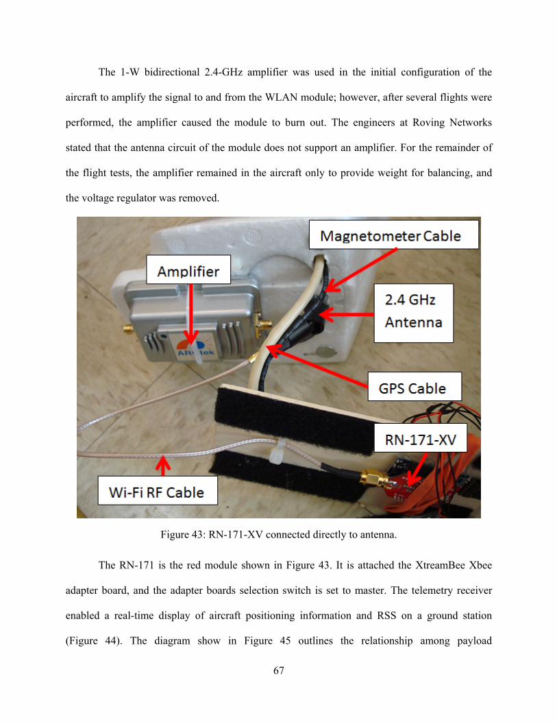
67
The 1-W bidirectional 2.4-GHz amplifier was used in the initial configuration of the
aircraft to amplify the signal to and from the WLAN module; however, after several flights were
performed, the amplifier caused the module to burn out. The engineers at Roving Networks
stated that the antenna circuit of the module does not support an amplifier. For the remainder of
the flight tests, the amplifier remained in the aircraft only to provide weight for balancing, and
the voltage regulator was removed.
Figure 43: RN-171-XV connected directly to antenna.
The RN-171 is the red module shown in Figure 43. It is attached the XtreamBee Xbee
adapter board, and the adapter boards selection switch is set to master. The telemetry receiver
enabled a real-time display of aircraft positioning information and RSS on a ground station
(Figure 44). The diagram show in Figure 45 outlines the relationship among payload
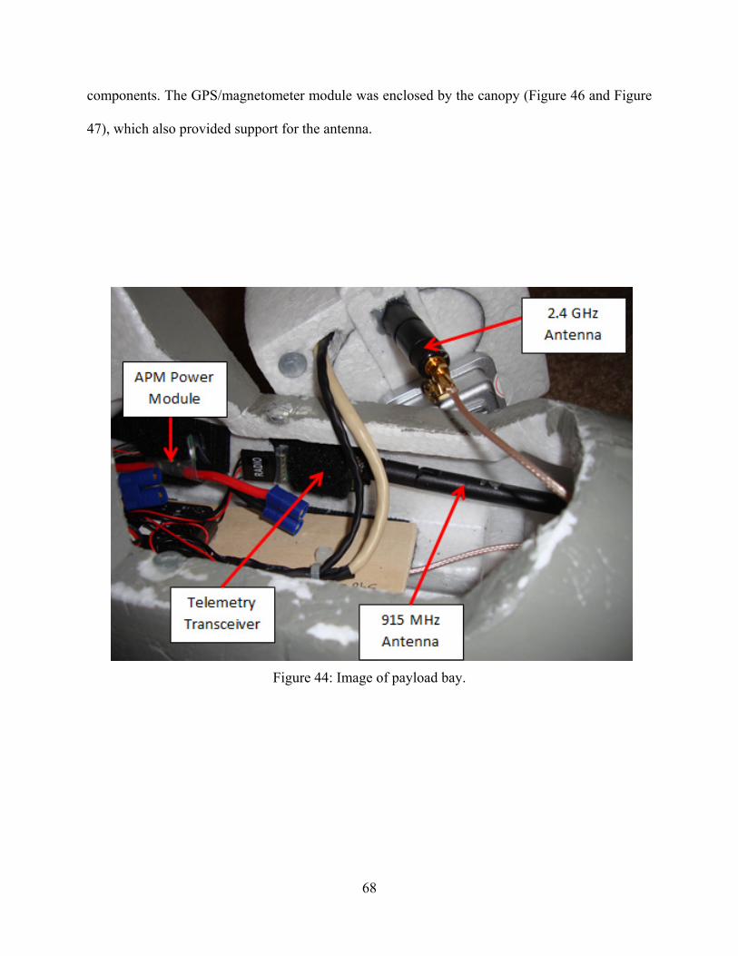
68
components. The GPS/magnetometer module was enclosed by the canopy (Figure 46 and Figure
47), which also provided support for the antenna.
Figure 44: Image of payload bay.
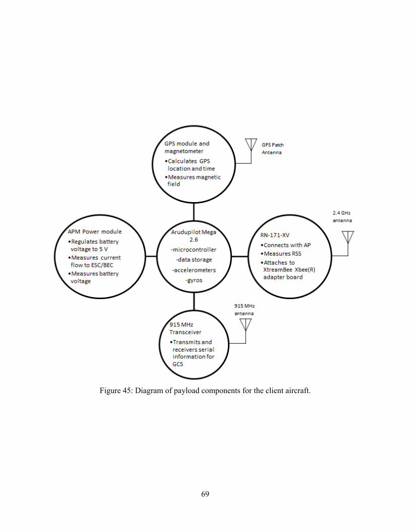
69
Figure 45: Diagram of payload components for the client aircraft.

70
Figure 46: GPS/magnetometer module and antenna.
Figure 47: Side view displaying antenna placement.

71
The APM power module supplies five volts to the microcontroller, which subsequently
provided five volts to the GPS module, telemetry transceiver, and WLAN module. The
microcontroller was modified from its standard configuration to allow access to two Universal
Asynchronous Receiver/Transmitter (UART) ports. UART0 port is shared by the USB™ port
and telemetry port. When the USB port is connected with a computer, the telemetry port is
disabled by an onboard multiplexer. UART2 port is accessible at the through-hole JP13 location
(Figure 48), and the pins adjacent to JP13 provide five volts and ground. UART2 was used to
communicate with the WLAN module (Figure 49).
Figure 48: UART2 connection.
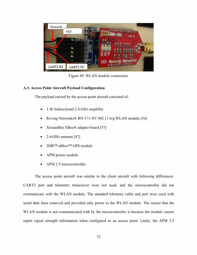
72
Figure 49: WLAN module connection.
A.3. Access Point Aircraft Payload Configuration
The payload carried by the access point aircraft consisted of:
1-W bidirectional 2.4-GHz amplifier
Roving Networks® RN-171-XV 802.11 b/g WLAN module [56]
XtreamBee XBee® adapter board [57]
2.4-GHz antenna [47]
3DR™ uBlox™ GPS module
APM power module
APM 2.5 microcontroller
The access point aircraft was similar to the client aircraft with following differences.
UART2 port and telemetry transceiver were not used, and the microcontroller did not
communicate with the WLAN module. The standard telemetry cable and port were used with
serial data lines removed and provided only power to the WLAN module. The reason that the
WLAN module is not communicated with by the microcontroller is because the module cannot
report signal strength information when configured as an access point. Lastly, the APM 2.5

73
contains the magnetometer onboard, while the GPS module is external. Figure 50outlines the
relationship among payload components.
Figure 50: Diagram of payload for access point aircraft.
A.4. Using APM autopilot feature
The APM is capable of flying the aircraft in addition to measuring signal strength data.
However, using the code written for this research, problems with the WLAN module will cause
the APM’s main processor to run a continuous loop in which the processor is looking for data
from the WLAN module. Since this loop does not contain the navigation or control functions, the
APM will not update flight control surfaces and may cause the plane to crash. The APM 2.5 and
2.6 do not contain a failsafe multiplexer. Consequently, if the processor runs into an infinite loop
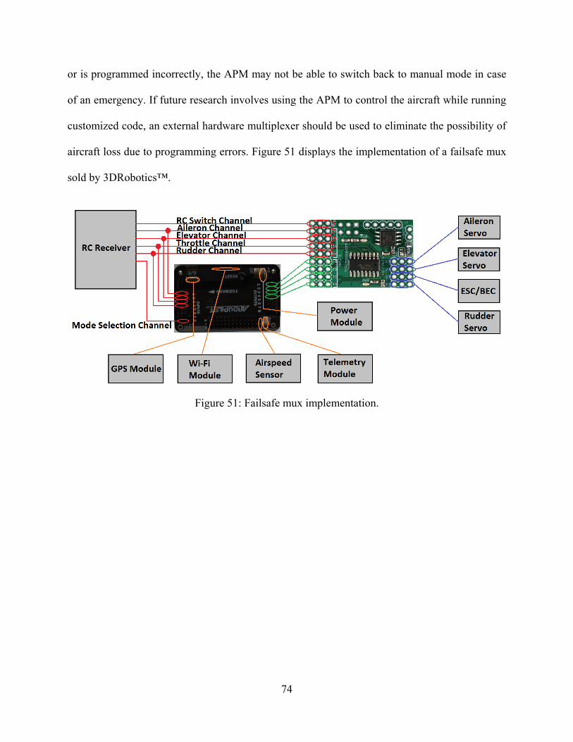
74
or is programmed incorrectly, the APM may not be able to switch back to manual mode in case
of an emergency. If future research involves using the APM to control the aircraft while running
customized code, an external hardware multiplexer should be used to eliminate the possibility of
aircraft loss due to programming errors. Figure 51 displays the implementation of a failsafe mux
sold by 3DRobotics™.
Figure 51: Failsafe mux implementation.

75
Appendix B. Software Configuration
In order to collect the data necessary for this research, the ArduPlane V2.75beta2 source
code [58] was modified, and the WLAN modules were manually configured. Section B.1
discusses the modifications made to the original ArduPlane source code in order to collect the
received signal strength (RSS). Section B.2 describes the setup process for the WLAN modules,
and Section B.3 illustrates how troubleshooting was performed.
B.1. ArduPlane source code modifications
The ArduPlane source code configures the ArduPilot as an autopilot for fixed-wing
aircraft. Modifications were made to the ArduPlane source code installed on the aircraft to
include a client WLAN module. Minor modifications were made to the ArduPlane code so as to
not disrupt the original ArduPlane routines. The WLAN module was originally connected to the
standard telemetry port. To collect WLAN data, the flow of telemetry data through this port must
be stopped. However, stopping telemetry data flow also stops data flow through the USB.
Consequently, the Mission Planner ground control software [58] is unable to communicate with
board. For this reason, the original configuration was abandoned, and the WLAN module was
connected to the UART2 port, which is the only other available port on the board. This
configuration allowed communications through the standard telemetry port and USB to remain
functional.
The Arduino programming language requires a void setup function and void loop
function. The setup function initializes the board in preparation for the loop function. The setup
function runs whenever power is connected to the ArduPilot, the reset button is pressed, or USB
port is connected or disconnected from a computer. Within this function, a command is sent to
the WLAN module requesting a reboot. This ensures that the module will be in the same state

76
every time the setup function runs. Following the reboot command is a command to place the
module in command mode, which is necessary to acquire RSS. Algorithm 1 is a section of
WifiTestConfiguration.ino, and the additions to this file are highlighted in red.
Algorithm 1: Additional Code added to setup function (WifiTestConfiguration.ino).
void setup() // this needs to be the first call, as it fills memory with // sentinel values memcheck_init(); cliSerial = hal.console; // load the default values of variables listed in var_info[] AP_Param::setup_sketch_defaults(); // arduplane does not use arming nor pre-arm checks notify.init(); AP_Notify::flags.armed = true; AP_Notify::flags.pre_arm_check = true; rssi_analog_source = hal.analogin->channel(ANALOG_INPUT_NONE); vcc_pin = hal.analogin->channel(ANALOG_INPUT_BOARD_VCC); batt_volt_pin = hal.analogin->channel(g.battery_volt_pin); batt_curr_pin = hal.analogin->channel(g.battery_curr_pin); init_ardupilot(); // initialise the main loop scheduler scheduler.init(&scheduler_tasks[0], sizeof(scheduler_tasks)/sizeof(scheduler_tasks[0])); hal.uartC->println_P(PSTR("reboot"));//Reboot WLAN adapter delay(500); hal.uartC->print_P(PSTR("$$$")); //Place WLAN adapter in command mode delay(500); The void loop function is the main program which runs continuously after initialization
has been performed. This loop contains a scheduler which allots time for the multiple tasks and
ensures that control updates are made at 50 Hz. Within this schedule is a logging task which
stores telemetry data to the onboard memory. Log.pde comprises the code used for logging (see
Figure 2). In Algorithm 2, modifications are highlighted in red. The character string mystring
was declared in the beginning of WifiTestConfiguration.ino. Since the RSS data must be logged
with the corresponding attitude data to meet data collection requirement, the commands to

77
acquire data from the WLAN module were placed within the function which logs the attitude
data to the memory. In this code, the show r command is routinely sent to the WLAN module,
and the module sends back a text string. This string is then parsed to pull out the RSS. The RSS
is then stored as an integer, and this value is logged with the rest of the data in the attitude
packet.
Algorithm 2: Code which requests and stores RSS data (Log.pde)
// Write an attitude packet. Total length : X bytes // Modified by Matthew Vincie static void Log_Write_Attitude(void) uint16_t stored_rssi; while(!hal.uartC->available())//Wait for input from modem hal.uartC->flush(); //Flush buffer for UART2 hal.uartC->println_P(PSTR("show r"));//Request RSS from modem for(int i=0;i<14;i++) while(!hal.uartC->available()) mystring[i]=hal.uartC->read();//Places modem reply in mystring stored_rssi=((mystring[7]-'0')*10+(mystring[8]-'0'));//Pulls the RSS // value from the string and stores the value as an integer receiver_rssi=stored_rssi*255/100; //This scaled value is sent to the GCS struct log_Attitude pkt = LOG_PACKET_HEADER_INIT(LOG_ATTITUDE_MSG), roll : (int16_t)ahrs.roll_sensor, pitch : (int16_t)ahrs.pitch_sensor, yaw : (uint16_t)ahrs.yaw_sensor, rssi : stored_rssi //RSS value added to the data being stored to //the APM memory ; DataFlash.WriteBlock(&pkt, sizeof(pkt)); The original ArduPlane source code is designed to measure RC receiver RSS and send
these values to the ground control station (GCS). Some RC receivers will output a voltage that is
proportional to the RSS. The ArduPilot uses an analog-to-digital converter on pins A0, A1, or
A13 to measure the voltage coming from RC receiver. The measured voltage is stored in the
receiver_rssi variable which is continuously updated with each measurement and then sent
within the telemetry stream to the GCS. The parameter list provides the ability to select the pin

78
used in the RSS measurement and to disable the RSS measurement altogether. When the RSS
measurement is disabled, the receiver_rssi variable will not update from zero; however, this
value is still sent to the GCS. The modified code updates the receiver_rssi variable with a scaled
value of the WLAN module’s RSS. This allows real-time display of the RSS to the GCS.
Lastly, the log structure for attitude was modified to contain the RSS variable. This was
done by adding an additional “c” before the final “C” within the log attitude structure (Algorithm
3).
Algorithm 3: Modification to attitude log structure (Log.pde).
static const struct LogStructure log_structure[] PROGMEM = LOG_COMMON_STRUCTURES, LOG_ATTITUDE_MSG, sizeof(log_Attitude), "ATT", "cccC", "Roll,Pitch,Yaw,RSSI" ,//An additional c was //added //before the final C to allow a slot for RSSI to be stored LOG_PERFORMANCE_MSG, sizeof(log_Performance), "PM", "IHhBBBhhhhB", "LTime,MLC,gDt,RNCnt,RNBl,GPScnt,GDx,GDy,GDz,I2CErr" , LOG_CMD_MSG, sizeof(log_Cmd), "CMD", "BBBBBeLL", "CTot,CNum,CId,COpt,Prm1,Alt,Lat,Lng" , LOG_CAMERA_MSG, sizeof(log_Camera), "CAM", "ILLeccC", "GPSTime,Lat,Lng,Alt,Roll,Pitch,Yaw" , LOG_STARTUP_MSG, sizeof(log_Startup), "STRT", "BB", "SType,CTot" , LOG_CTUN_MSG, sizeof(log_Control_Tuning), "CTUN", "cccchhf", "NavRoll,Roll,NavPitch,Pitch,ThrOut,RdrOut,AccY" , LOG_NTUN_MSG, sizeof(log_Nav_Tuning), "NTUN", "CICCcc", "Yaw,WpDist,TargBrg,NavBrg,AltErr,Arspd" , LOG_MODE_MSG, sizeof(log_Mode), "MODE", "MB", "Mode,ModeNum" , LOG_CURRENT_MSG, sizeof(log_Current), "CURR", "hhhHf", "Thr,Volt,Curr,Vcc,CurrTot" , LOG_COMPASS_MSG, sizeof(log_Compass), "MAG", "hhhhhhhhh", "MagX,MagY,MagZ,OfsX,OfsY,OfsZ,MOfsX,MOfsY,MOfsZ" , TECS_LOG_FORMAT(LOG_TECS_MSG), ;

79
B.2. WLAN module setup process
Setting up the WLAN modules is a two-step process. The firmware on each module was
first updated to wifly-EZX version 4.00.1. The updated firmware allows the module to function
as an access point and includes bug fixes. The second step is to configure the individual modules
to perform in the WLAN network. Section B.2.1 describes the method used to update the
firmware, and Section B.2.2 outlines the process of configuring the individual modules. For
additional information, visit the Microchip website.
B.2.1. WLAN module firmware update
Before the firmware on the module can be updated, the module must be able to
communicate with a computer. Communication can be achieved in three ways: using an
XtreamBee Xbee adapter board with a FTDI cable, Ad-hoc wireless connection, or RN-XV-EK1
USB serial converter with USB cable. The XtreamBee Xbee method requires moving the solder
jumper on the board to allow for a 3.3 V input. Of these methods, the serial converter method
provides the easiest setup. This method was used in this research.
Once the module is connected to the computer either by USB or FTDI, communication
with the module is done through a terminal emulator which is able to communicate through a
serial port. For this research, Tera Term version 4.78 was used, which has features similar to
PuTTY and SecureCRT. Tera Term is open source software and can be downloaded from the
TeraTerm Project website.
When starting the Tera Term, the serial port associated with the WLAN module must be
selected (Figure 52).

80
Figure 52: Serial port selection in Tera Term.
After clicking OK, press the reset button on the RN-XV-EK1 board. You should see information
similar to that shown in Figure 53.
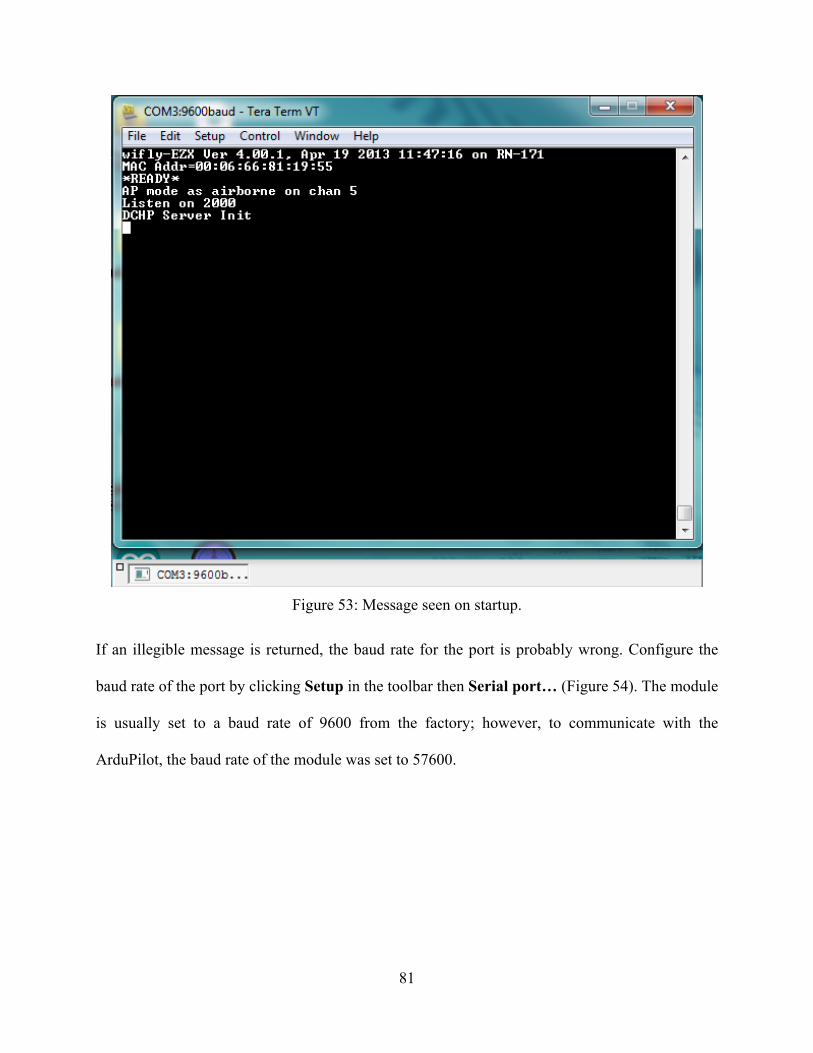
81
Figure 53: Message seen on startup.
If an illegible message is returned, the baud rate for the port is probably wrong. Configure the
baud rate of the port by clicking Setup in the toolbar then Serial port… (Figure 54). The module
is usually set to a baud rate of 9600 from the factory; however, to communicate with the
ArduPilot, the baud rate of the module was set to 57600.

82
Figure 54: Setting baud rate for serial port.
After a legible message has been received from the module, the firmware update process can
begin.
The next step is to place the module in command mode by typing $$$ in the terminal
window together quickly without additional characters directly before or after. The module will
then return CMD. Type factory R to reset the module to factory specifications. Then type scan
to see which wireless access points are available. If the wireless access point has a password,
type set w p password, where password is the password for the wireless access point. Next type
join SSID, where SSID is the SSID of the access point you are trying to join. This access point
must have internet access for firmware update, and the SSID must not have any spaces between
characters. Type ftp update to download and update the firmware. After the update, type reboot,

83
and place the module in command mode again. Type factory R, then type save, and lastly type
reboot. The module is now ready for manual configuration.
B.2.2. WLAN module configuration
To configure the module which functions as the access point in the network, start by
placing the module in command mode. Type set wlan join 7 or set w j 7 (short notation), to
enable AP mode. Next type set w c 5 to specify wireless communication on 802.11 channel 5.
Type set w s airborne (airborne is the access point SSID). Then type set i d 4 which enables the
DHCP server. Next type set w r 0 which reduces the wireless data rate to 1 Mbits/s which is the
slowest rate available and maximizes the transmission distance. The final step is to save the
configuration. Type save filename, where filename is the name you would like to use for the
configuration file. Multiple configuration files can be saved and loaded from the internal
memory. If you run into an error saving the file, make sure that you performed a factory reset
before beginning the configuration. Lastly type save which will overwrite the running
configuration file (config). The module is now ready to be rebooted and used. Appendix C shows
a list of all the configuration parameters for the access point.
To configure the module which functions as the client in the network, place the module in
command mode. Type set w s SSID, where SSID is the SSID of the access point which will be
automatically connected upon startup. The current firmware does not allow the access point to
have a password, so the password stored on the client module is irrelevant. Next type set w r 0 to
set the wireless data rate. Then type set w j 1 to configure the module to automatic login to the
access point. Now type set u b 57600 which allows the module to communicate with the
ArduPilot at the baud rate of 57600. When the module is rebooted, the baud rate in Tera Term
must be adjusted. Next type set w a 0 which specifies that the access point which the client is
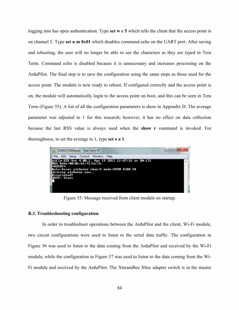
84
logging into has open authentication. Type set w c 5 which tells the client that the access point is
on channel 5. Type set u m 0x01 which disables command echo on the UART port. After saving
and rebooting, the user will no longer be able to see the characters as they are typed in Tera
Term. Command echo is disabled because it is unnecessary and increases processing on the
ArduPilot. The final step is to save the configuration using the same steps as those used for the
access point. The module is now ready to reboot. If configured correctly and the access point is
on, the module will automatically login to the access point on boot, and this can be seen in Tera
Term (Figure 55). A list of all the configuration parameters is show in Appendix D. The average
parameter was adjusted to 1 for this research; however, it has no effect on data collection
because the last RSS value is always used when the show r command is invoked. For
thoroughness, to set the average to 1, type set o a 1.
Figure 55: Message received from client module on startup.
B.3. Troubleshooting configuration
In order to troubleshoot operations between the ArduPilot and the client, Wi-Fi module,
two circuit configurations were used to listen to the serial data traffic. The configuration in
Figure 56 was used to listen to the data coming from the ArduPilot and received by the Wi-Fi
module, while the configuration in Figure 57 was used to listen to the data coming from the Wi-
Fi module and received by the ArduPilot. The XtreamBee Xbee adapter switch is in the master

85
position for both configurations. Tera Term is used to display the serial data stream on the
connected computer.
Figure 56: Configuration to listen to data coming from ArduPilot.
Figure 57: Configuration to listen to data coming from Wi-Fi module.

86
Appendix C. Access point Configuration Parameters.
<4.00> get e wifly-EZX Ver 4.00.1, Apr 19 2013 11:47:20 on RN-171 Beacon=102 Reboot=0 IF=UP DHCP=SERVER IP=0.0.0.0:2000 NM=255.255.255.0 GW=0.0.0.0 HOST=0.0.0.0:2000 PROTO=TCP, MTU=1524 FLAGS=0x7 TCPMODE=0x0 BACKUP=0.0.0.0 OPEN=*OPEN* CLOSE=*CLOS* REMOTE=*HELLO* FlushSize=1420 MatchChar=0 FlushTimer=5 IdleTimer=0 CmdChar=$ DNS=0.0.0.0 Name=dns1 Backup=rn.microchip.com Lease=86400 FTP=0.0.0.0:21 File=wifly-EZX.img User=roving Pass=Pass123 Dir=public Timeout=200 FTP_mode=0x0 SSID=airborne Chan=5 ExtAnt=0 Join=7 Auth=OPEN Mask=0x1fff Rate=0, 1 Mb Linkmon-Infra=30 Linkmon-AP=3600 Passphrase=rubygirl TxPower=12 EAP_Id=userid EAP_User=peap-user SleepTmr=0 WakeTmr=0

87
Trigger=0x1 Autoconn=0 IoFunc=0x0 IoMask=0x21f0 IoValu=0x0 DebugReg=0x0 PrintLvl=0x1 LaunchStr=web_app TimeEna=0 TIMEADR=64.90.182.55:123 Zone=7 Baudrate=9600 Flow=0x0 Mode=0x0 Cmd_GPIO=0 JoinTmr=1000 Replace=0x24 DeviceId=WiFly-EZX Password= Format=0x0 Signal=0 Average=5 BCAST=255.255.255.255:55555 Interval=0x7 Backup=0.0.0.0:0 Sensor=0x0 SensePwr=0x0 <4.00>

88
Appendix D. Client Configuration Parameters
<4.00> get e wifly-EZX Ver 4.00.1, Apr 19 2013 11:47:20 on RN-171 Beacon=102 Reboot=0 IF=UP DHCP=ON IP=0.0.0.0:2000 NM=0.0.0.0 GW=0.0.0.0 HOST=0.0.0.0:2000 PROTO=TCP, MTU=1524 FLAGS=0x7 TCPMODE=0x0 BACKUP=0.0.0.0 OPEN=*OPEN* CLOSE=*CLOS* REMOTE=*HELLO* FlushSize=1420 MatchChar=0 FlushTimer=5 IdleTimer=0 CmdChar=$ DNS=0.0.0.0 Name=dns1 Backup=rn.microchip.com Lease=86400 FTP=0.0.0.0:21 File=wifly-EZX.img User=roving Pass=Pass123 Dir=public Timeout=200 FTP_mode=0x0 SSID=airborne Chan=0 ExtAnt=0 Join=1 Auth=OPEN Mask=0x1fff Rate=0, 1 Mb Linkmon-Infra=30 Linkmon-AP=3600 Passphrase=open TxPower=12 EAP_Id=userid EAP_User=peap-user SleepTmr=0 WakeTmr=0

89
Trigger=0x1 Autoconn=1 IoFunc=0x0 IoMask=0x21f0 IoValu=0x0 DebugReg=0x0 PrintLvl=0x1 LaunchStr=web_app TimeEna=0 TIMEADR=64.90.182.55:123 Zone=7 Baudrate=57600 Flow=0x0 Mode=0x1 Cmd_GPIO=0 JoinTmr=1000 Replace=0x24 DeviceId=WiFly-EZX Password= Format=0x0 Signal=92 Average=1 BCAST=255.255.255.255:55555 Interval=0x7 Backup=0.0.0.0:0 Sensor=0x0 SensePwr=0x0 <4.00>

90
Appendix E. Supporting Figures
This appendix contains figures from all three scenarios and supports the results section of
this thesis.
E.1. Air-to-Air Scenario Figures
Figure 58: RSS vs. Time for AtoA Scenario using Raw Heading.
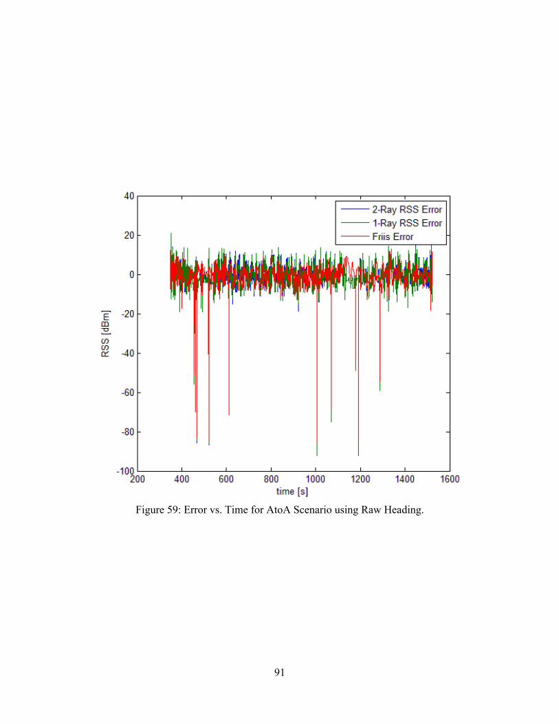
91
Figure 59: Error vs. Time for AtoA Scenario using Raw Heading.

92
Figure 60: Scatter Plot of Error vs. Distance for AtoA Scenario using Raw Heading.
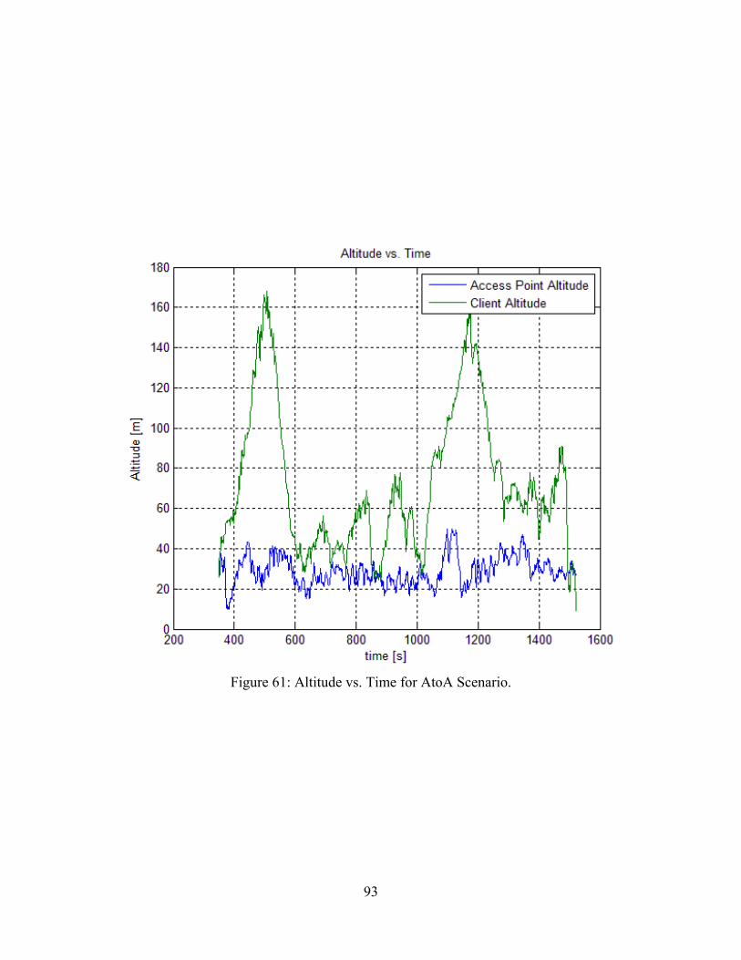
93
Figure 61: Altitude vs. Time for AtoA Scenario.
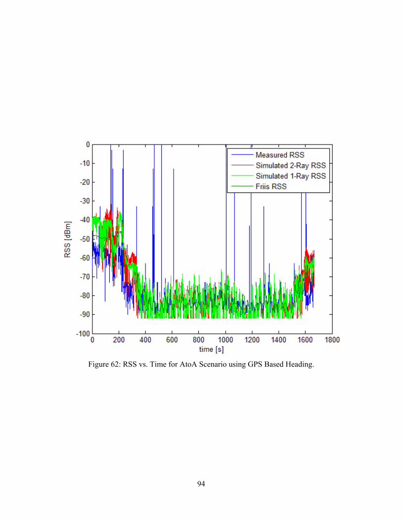
94
Figure 62: RSS vs. Time for AtoA Scenario using GPS Based Heading.

95
Figure 63: Error vs. Time for AtoA Scenario using GPS Based Heading.

96
Figure 64: Error vs. Distance for AtoA Scenario using GPS Based Heading.

97
Figure 65: Statistical Analysis of AtoA Scenario with GPS Based Heading.
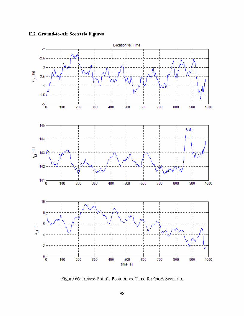
98
E.2. Ground-to-Air Scenario Figures
Figure 66: Access Point’s Position vs. Time for GtoA Scenario.

99
Figure 67: Distribution of x location of Access Point for GtoA Scenario.

100
Figure 68: Distribution of y location of Access Point for GtoA Scenario.
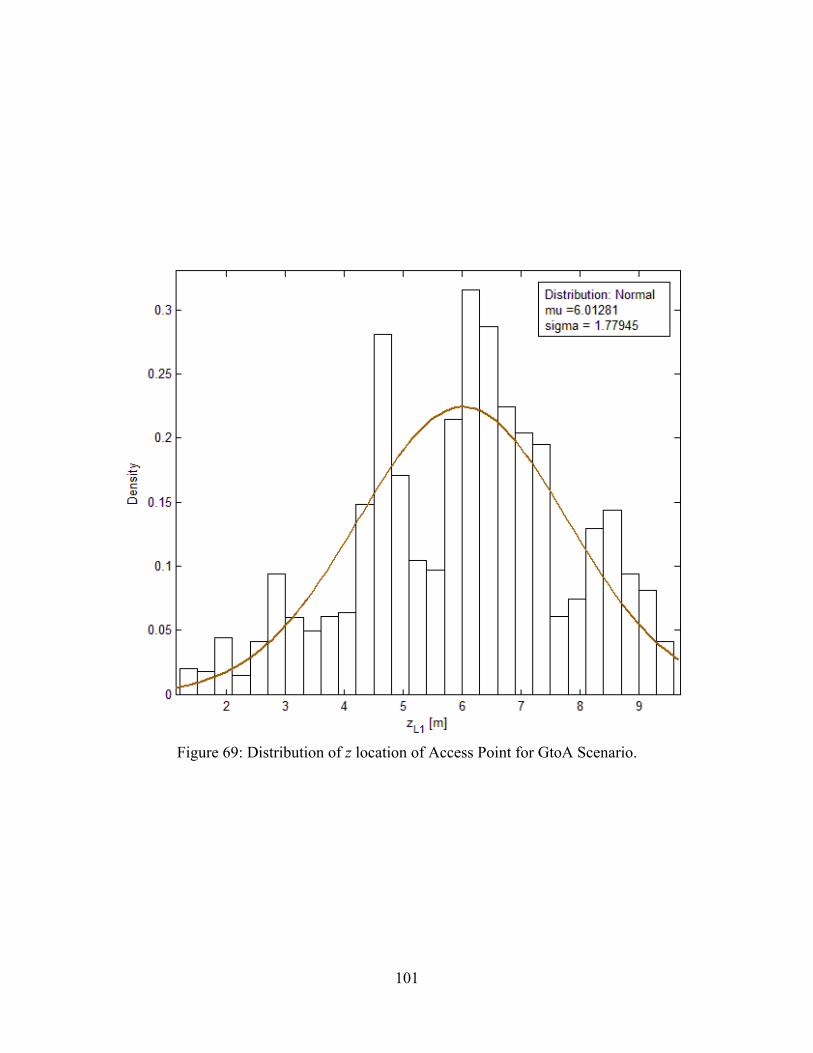
101
Figure 69: Distribution of z location of Access Point for GtoA Scenario.

102
Figure 70: Access Point’s Attitude Angles for GtoA Scenario.
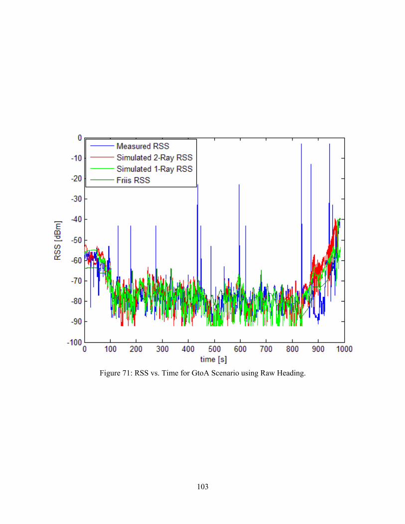
103
Figure 71: RSS vs. Time for GtoA Scenario using Raw Heading.

104
Figure 72: Error vs. Time for GtoA Scenario using Raw Heading.
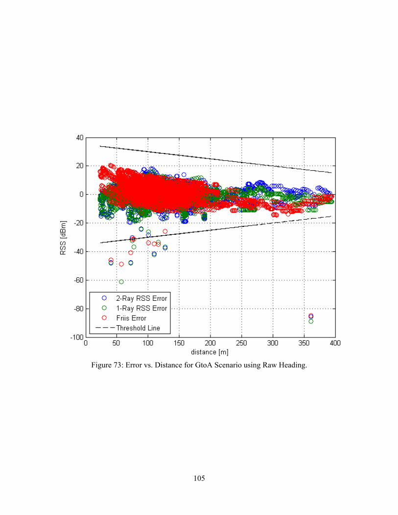
105
Figure 73: Error vs. Distance for GtoA Scenario using Raw Heading.

106
Figure 74: Altitude vs. Time for GtoA Scenario.
Figure 75: RSS vs. Time for GtoA Scenario using GPS Based Heading.

107
Figure 76: Error vs. Time for GtoA Scenario using GPS Based Heading.
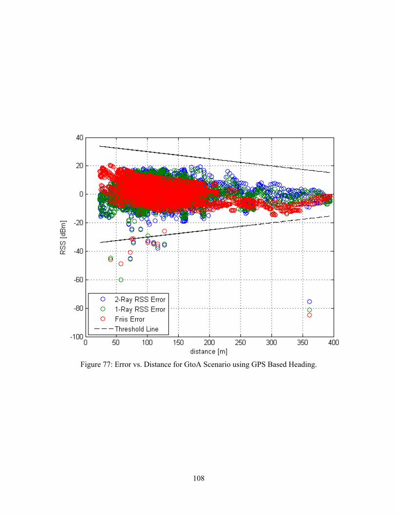
108
Figure 77: Error vs. Distance for GtoA Scenario using GPS Based Heading.
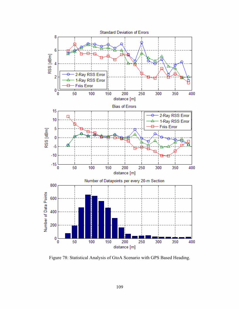
109
Figure 78: Statistical Analysis of GtoA Scenario with GPS Based Heading.
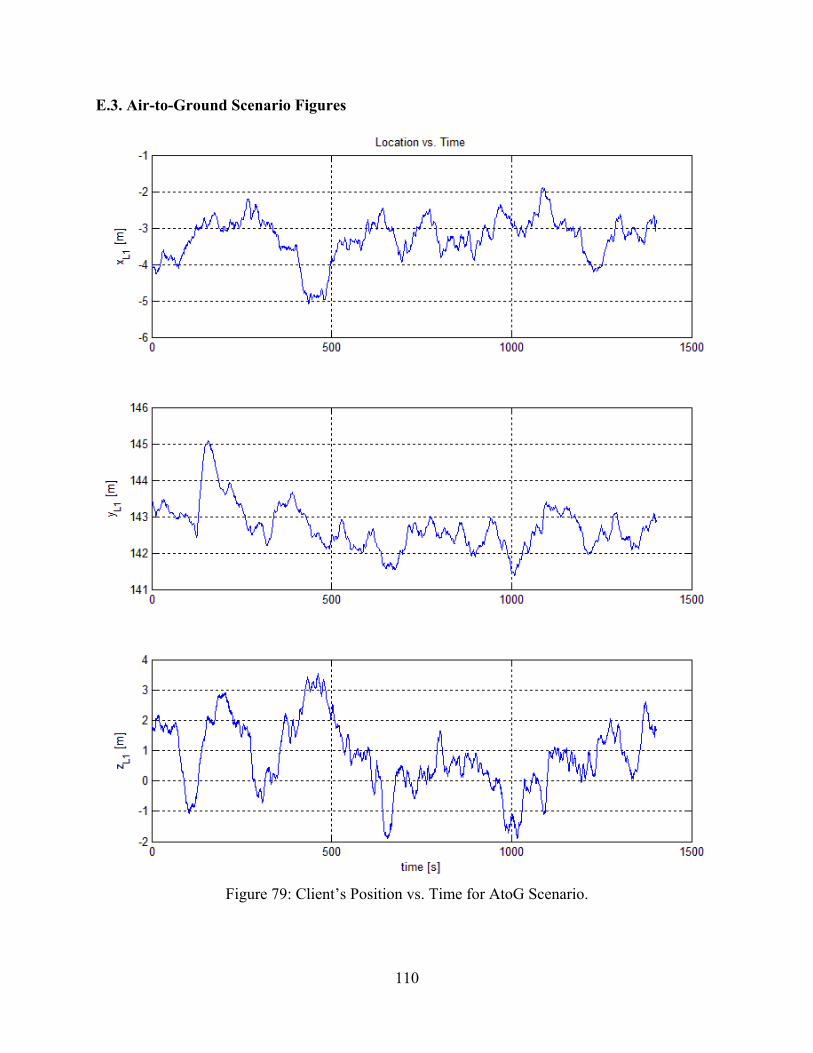
110
E.3. Air-to-Ground Scenario Figures
Figure 79: Client’s Position vs. Time for AtoG Scenario.

111
Figure 80: Distribution of x location of Client for AtoG Scenario.
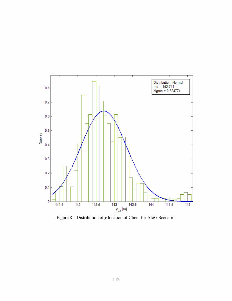
112
Figure 81: Distribution of y location of Client for AtoG Scenario.

113
Figure 82: Distribution of z location of Client for AtoG Scenario.

114
Figure 83: Client’s Attitude Angles for AtoG Scenario.
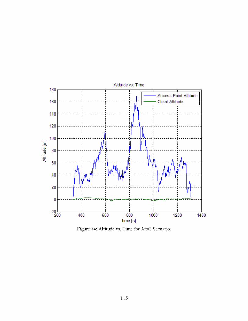
115
Figure 84: Altitude vs. Time for AtoG Scenario.
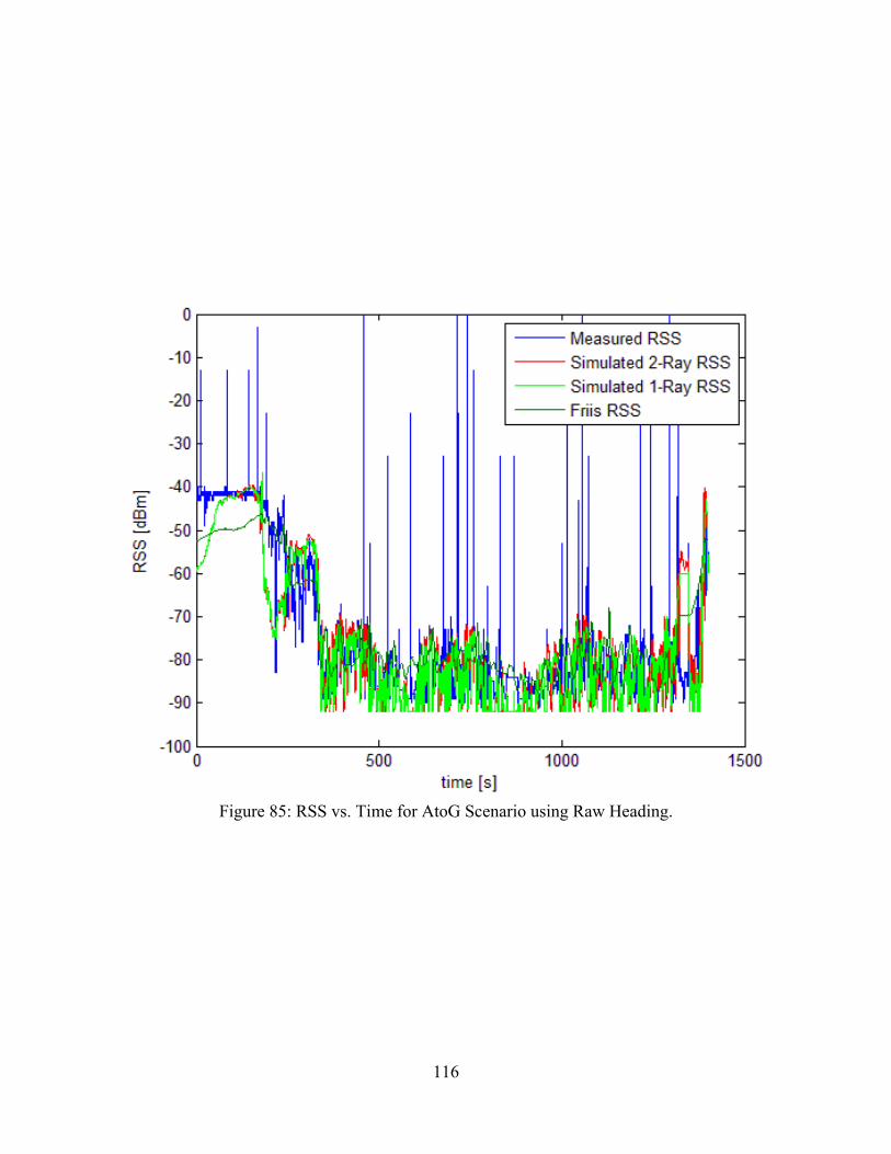
116
Figure 85: RSS vs. Time for AtoG Scenario using Raw Heading.
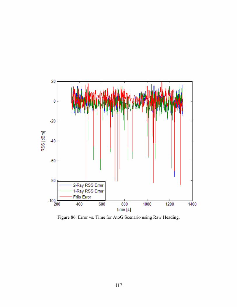
117
Figure 86: Error vs. Time for AtoG Scenario using Raw Heading.

118
Figure 87: Error vs. Distance for AtoG Scenario using Raw Heading.
Figure 88: RSS vs. Time for AtoG Scenario using GPS Based Heading.

119
Figure 89: Error vs. Time for AtoG Scenario using GPS Based Heading.

120
Figure 90: Error vs. Distance for AtoG Scenario using Raw Heading

121
.
Figure 91: Statistical Analysis of AtoG Scenario with GPS Based Heading.

122
E.4. Figures from all scenarios combined
Figure 92: Error vs. Distance for All Scenario using GPS Based Heading.

123
Figure 93: Error distribution of one-ray for all scenarios (data unit is dBm).
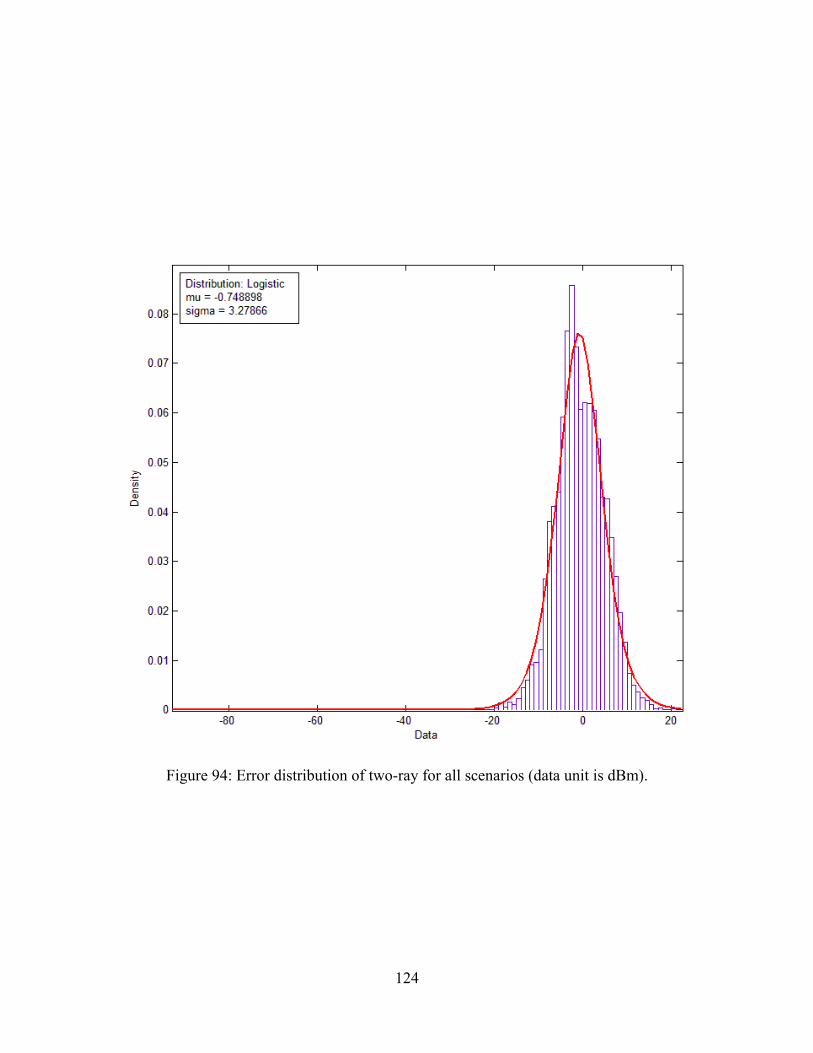
124
Figure 94: Error distribution of two-ray for all scenarios (data unit is dBm).
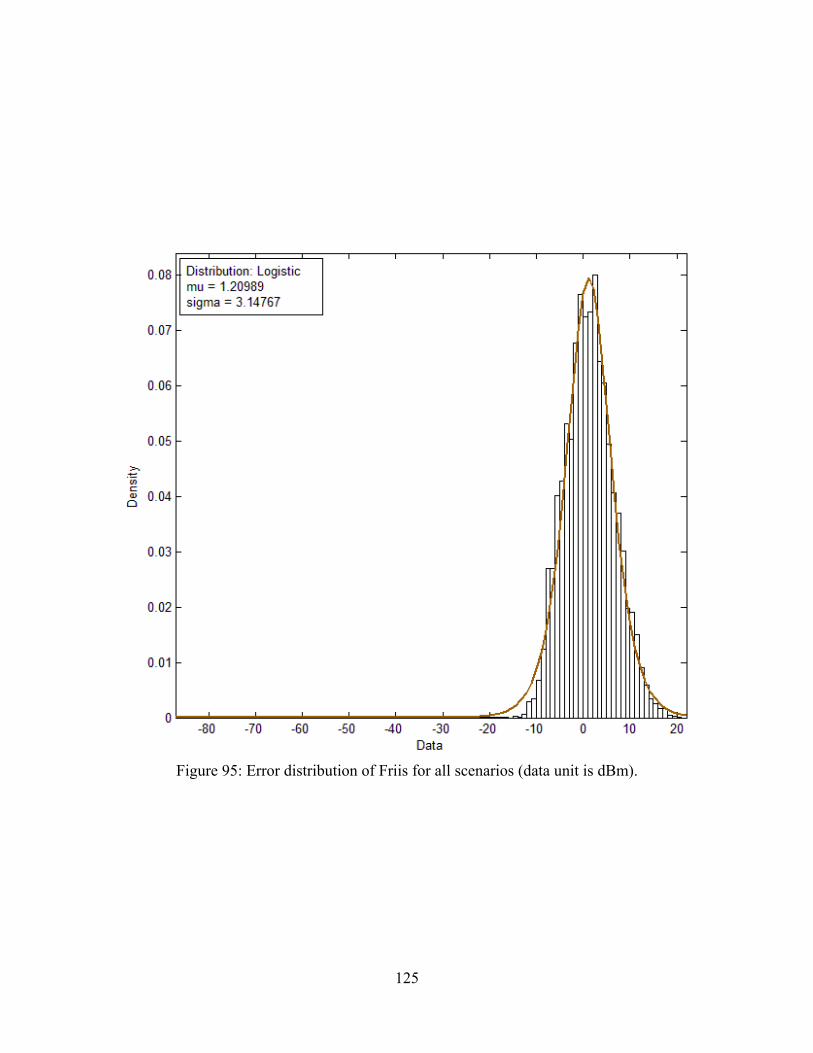
125
Figure 95: Error distribution of Friis for all scenarios (data unit is dBm).
126
Bibliography
[1] R. Lee, J. Manner, J. Kim, B. Hurley, P. Amodio, and K. Anderson, ”The role of deployable aerial communications architecture in emergency communications and recommended next steps,” Federal Communications Commission, Washington, DC, White Paper DOC-309742A1. September 2011.
[2] K. Pawlikowski, H.-D.J. Jeong, and J.-S.R. Lee, "On credibility of simulation studies of
telecommunication networks," IEEE Communications Magazine, vol. 40, no. 1, pp. 132-139, 2002. DOI: 10.1109/35.978060.
[3] L. F. Perrone, D. Nicol, and Yuan Yougu, "Modeling and simulation best practices for
wireless ad hoc networks," in Proc. of the 2003 Winter Simulation Conference, vol. 1, pp. 685-693, 2003. DOI: 10.1109/WSC.2003.1261484.
[4] S. Kurkowski, T. Camp, and M. Colagrosso, "Manet simulation studies: the current state and
new simulation tools," Technical Report MCS 06-01, Colorado School of Mines, pp. 1-13, Feb 2006.
[5] T. R. Andel and A. Yasinsac, "On the credibility of manet simulations," Computer ,vol. 39,
no. 7, pp. 48-54, 2006. [6] J. H. Hansen, ”Optimal guidance of a relay mav for isr support beyond line-of-sight.” MS
Thesis, AFIT/GAE/ENG/08-01, Air Force Institute of Technology, Wright-Patterson AFB, OH. 27 March 2008.
[7] M. T. Seibert, A. J. Stryker, J. R. Ward, and C. T. Wellbaum, ”System analysis and
prototyping for single operator management of multiple unmanned aerial vehicles operating beyond line of sight.” MS Thesis, AFIT/GSE/ENV/10-M01, Air Force Institute of Technology, Wright-Patterson AFB, OH, 26 March 2010.
[8] J. P. Boire, ”Autonomous routing of unmanned aerial vehicle (UAV) relays to mimic optimal
trajectories in real time.” MS Thesis, AFIT/GSE/ENV/11-M03, Air Force Institute of Technology, Wright-Patterson AFB, OH, 24 March 2011.
[9] T. J. Shuck, ”Development of autonomous optimal cooperative control in relay rover
configured small unmanned aerial systems.” MS Thesis. AFIT-ENV-13-M-27, Air Force Institute of Technology, Wright-Patterson AFB, OH, 21 March 2013.
[10] S. A. Songer, ”Aerial networking for the implementation of cooperative control on small
unmanned.” MS Thesis. AFIT-ENV-13-M-29, Air Force Institute of Technology, Wright-Patterson AFB, OH. 21 March 2013.
127
[11] C. M. Durham, ”Evaluation of an OPNET model for unmanned aerial vehicle networks.” MS Thesis. AFIT/GCO/ENG/09-04, Air Force Institute of Technology, Wright-Patterson AFB, OH. 26 March 2009.
[12] K. Daniel, S. Rohde, N. Goddemeier, and C. Wietfeld, ”Cognitive agent mobility for aerial
sensor networks,” IEEE Sensors Journal, vol. 11 ,no. 11, pp. 2671-2682. 2011. DOI: 10.1109/JSEN.2011.2159489.
[13] S. Morgenthaler, T. Braun, Z. Zhongliang, T. Staub, and M. Anwander, ”UAVNet: A
mobile wireless mesh network using unmanned aerial vehicles,” in Proc. of 2012 IEEE Globecom Workshops, pp. 1603-1608, 2012. DOI: 10.1109/GLOCOMW.2012.6477825.
[14] T. Stoyanova, F. Kerasiotis, A. Prayati, and G. Papadopoulos, ”Communication-aware
deployment for wireless sensor networks,” in Proc of Second International Conference on Sensor Technologies and Applications, pp. 217-222, 2008. DOI: 10.1109/SENSORCOMM.2008.97.
[15] D. P. Horner and A. J. Healey, ”Use of artificial potential fields for UAV guidance and
optimization of WLAN communications,” in Proc. Of IEEE/OES 2004 Autonomous Underwater Vehicles Conference, pp. 88-95, 2004. DOI: 10.1109/AUV.2004.1431198.
[16] Z. Pengcheng, Y. Kai, and A. Swindlehurst, ”Wireless relay communications using an
unmanned aerial vehicle,” in Proc. of IEEE 7th Workshop on Signal Processing Advances in Wireless Communications. pp. 1-5, 2006. DOI: 10.1109/SPAWC.2006.346492.
[17] C. Chen-Mou, P. Hsiao, H. Kung, and D. Vlah, ”Transmit antenna selection based on link-
layer channel probing,” in Proc. of World of Wireless Mobile and Multimedia Networks 2007 IEEE International Symposium, pp. 1-6, 2007. DOI: 10.1109/WOWMOM.2007.4351703.
[18] G. Hadynski, S. Lee, G. Rajappan, R. Sundaram, X. Wang, and F. Zhou, ”Optimization of
directional antenna network topology in airborne networks,” in Proc. of 2010 Military Communications Conference. pp. 68-73, 2010. DOI: 10.1109/MILCOM.2010.5680269.
[19] C. E. Lin, Y. Huang, Y. Lai, Y. Yeh, and W. Huang, ”Airborne antenna tracking for sky-net
mobile communication,” in Proc. of 2011 Fifth International Conference on Sensing Technology, pp. 569-574, 2011. DOI: 10.1109/ICSensT.2011.6137044.
[20] A. Ayyagari, J. Harrang, and S. Ray, ”Airborne information and reconnaissance network,”
in Proc. of 1996 Military Communications Conference, vol. 1, pp. 230-234, 1996. DOI: 10.1109/MILCOM.1996.568619.
[21] H. T. Kung, C. Lin, T. Lin, S. Tarsa, and D. Vlah, ”Measuring diversity on a low-altitude
UAV in a ground-to-air wireless 802.11 mesh network,” in Proc. of GLOBECOM Workshops, pp. 1799-1804, 2010. DOI: 10.1109/GLOCOMW.2010.5700251.

128
[22] E. K. Çetinkaya, J. Rohrer, A. Jabbar, M. Alenazi, D. Zhang, D. Broyles, K. Pathapati, H. Narra, K. Peters, S. Gogi, and J. Sterbenz, ”Protocols for highly-dynamic airborne networks,” in Proc. of the 18th Annual International Conference on Mobile Computing and Networking, pp. 411-414. 2012. DOI: 10.1145/2348543.2348597
[23] C. Cheng, P. Hsiao, H. Kung, and D. Vlah, ”Maximizing throughput of UAV-relaying
networks with the load-carry-and-deliver paradigm,” in Proc. of Wireless Communications and Networking Conference, pp. 4417-4424, 2007. DOI: 10.1109/WCNC.2007.805.
[24] A. Sivakumar, T. Phang, C. Tan, and W. Seah, ”Robust airborne wireless backbone using
low-cost UAVs and commodity WiFi technology,” in Proc. of 8th International Conference on ITS Telecommunications. pp. 373-378, 2008. DOI: 10.1109/ITST.2008.4740289.
[25] H. T. Kung, ”Research and demonstration of video streaming on unmanned aerial vehicles
(UAV) networks.” Harvard University, Cambridge, MA, 2008. [26] C. Danilov, T. Henderson, T. Goff, J. Kim, J. Weston, N. Neogi, A. Ortiz, and D. Uhlig,
”Experiment and field demonstration of a 802.11-based ground-UAV mobile ad-hoc network,” in Proc. in 2009 Military Communications Conference, pp. 1-7, 2009. DOI: 10.1109/MILCOM.2009.5379932.
[27] D. Hague. H. Kung, and B. Suter, ”Field experimentation of cots-based UAV networking,”
in Proc. of 2006 Military Communications Conference, pp. 1-7. 2006. DOI: 10.1109/MILCOM.2006.302070.
[28] J. Allred, A. Hasan, S. Panichsakul, W. Pisano, P. Gray, J. Huang, R. Han, D. Lawrence,
and K. Mohseni, ”SensorFlock: An airborne wireless sensor network of micro-air vehicles,” in Proc. of the 5th International Conference on Embedded Networked Sensor Systems, pp. 117-129, 2007.
[29] T. X. Brown, S. Doshi, S. Jadhav, and J. Himmelstein, ”Test bed for a wireless network on
small UAVs,” in Proc. of the 3rd AIAA “Unmanned Unlimited” Technical Conference, Chicago, IL, pp. 20-30, 2004.
[30] T. X. Brown, B. Argrow, C. Dixon, S. Doshi, R. Thekkekunnel, and D. Henkel, “Ad hoc
uav ground network (augnet),” in Proc. of AIAA 3rd Unmanned Unlimited Technical Conference. 2004. DOI: 10.2514/6.2004-6321.
[31] M. Gillen, J. Loyall, K. Usbeck, K. Hanlon, A. Scally, J. Sterling, R. Newkirk, R. Kohler,
”Beyond line-of-sight information dissemination for force protection,” in Proc. of 2012 Military Communications Conference, pp. 1-6. 2012. DOI: 10.1109/MILCOM.2012.6415700.
[32] T. M. Schulteis and J. G. Price, “Project stork UAV/UGV collaborative initiative,” Defense
and Security. International Society for Optics and Photonics, pp. 414-425, 2004.

129
[33] J. M. Grasmeyer and M. T. Keennon, ”Development of the black widow micro air vehicle”. Progress in Astronautics and Aeronautics, vol. 195, pp. 519-535. 2001.
[34] A. Ryan, M. Zennaro, A. Howell, R. Sengupta, and J. Hendrick, “An overview of emerging
results in cooperative UAV control,” in Proc. of 43rd IEEE Conference in Decision and Control. vol. 1, pp. 602-607, 2004. DOI: 10.1109/CDC.2004.1428700.
[35] U.S. Department of Defense, “DoD Releases Electromagnetic Spectrum Strategy,”
www.defense.gov/Releases, February 20, 2014, [Online]. Available: http://www.defense.gov/Releases/Release.aspx?ReleaseID=16547
[36] Riverbed, “OPNET IT Guru,” support.riverbed.com. [Online] Available:
https://support.riverbed.com/bin/support/static//doc/opnet/17.5.A/online/itguru_17.5.PL5/Modules/wwhelp/wwhimpl/js/html/wwhelp.htm#href=FA_10_Ov.060.1.html#47363 (Accessed: 12 March 2014)
[37] C. V. Chung, “Simulation of radiowave propagation in a dense urban environment,” MS
Thesis, Naval Postgraduate School, Monterey, CA, 2007. [38] Leidos, “Asymptotic Electromagnetic Radiation Software,” www.leidos.com. [Online]
Available: https://www.leidos.com/products/software/urbana (Accessed: 13 February 2014) [39] T. S. Rappaport, Wireless Communications: Principles and Practice,2nd ed., New Jersey,
Prentic Hall PTR, 1996. [40] K. Daniel, M. Putzke, B. Dusza, and C. Wietfeld, “Three dimensional channel
characterization for low altitude aerial vehicles,” in Proc. of 7th International Symposium on Wireless Communication Systems. pp. 756-760. 2010. DOI: 10.1109/ISWCS.2010.5624356.
[41] T. Stoyanova, F. Kerasiotis, A. Prayati, G. Papadopoulos, “A practical RF propagation
model for wireless network sensors,” in Proc. of 3rd International Conference on Sensor Technologies and Applications, pp. 194-199, 2009. DOI: 10.1109/SENSORCOMM.2009.39.
[42] N. Ahmed, S. Kanhere, and S. Jha, “Link characterization for aerial wireless sensor
networks,” in Proc. of 2011 IEEE GLOBECOM Workshops, pp. 1274-1279, 2011. DOI: 10.1109/GLOCOMW.2011.6162388.
[43] L. C. Kempel, “Computational Electromagnetics for Antennas” in Antenna engineering
handbook, 4th ed. J. L. Volakis, New York, McGraw-Hill Book Company, 1984, pp. 59.1-59.29.
[44] S. N. Makarov, Antenna and EM Modeling with MATLAB, vol. 1, Princeton University
Press, 2002.

130
[45] S. N. Makarov and L. C. Kempel, “MATLAB Antenna Toolbox. A Draft,” 2 February 2006, [Online], Available: http://ece.wpi.edu/mom/ (Accessed: 13 February 2014).
[46] CSGNetwork, “Length of a degree of latitude and longitude calculator,” CSGNetwork.com.
[Online] Available: http://www.csgnetwork.com/degreelenllavcalc.html (Accessed: 13 February 2014).
[47] TP-LINK Technology, “2.4GHz 8dBi indoor omni-directional antenna,” TL-ANT3408CL
datasheet, Available: http://www.tp-link.com/en/products/details/?model=TL-ANT2408CL#down.
[48] W. H. Hayt, Jr. and J. A. Buck , “Plane wave reflection and dispersion,” in Engineering
Electromagnetics, 7th ed., 2006, pp. 434-475. [49] S. S. Haykin and M. Moher, “Propagation and Noise,” in Modern Wireless Communication,
2004, pp. 11-94. [50] D. M. Dobkin, “Propagation,” in RF Engineering for Wireless Networks: Hardware,
Antennas, and Propagation, 2011, pp. 251-303. [51] H. R. Anderson, “Electromagnetic wave propagation,” in Fixed Broadband Wireless System
Design, 2003, pp. 25-68. [52] W. E. Patitz, B. C. Brock, and E. G. Powell, “Measurement of dielectric and magnetic
properties of soil,” Sandia National Labs, Albuquerque, NM, 1995. SAND95-2419 [53] S. M. Rao, D. Wilton, and A. W. Glisson, “Electromagnetic scattering by surfaces of
arbitrary shape," IEEE Transactions on Antennas and Propagation, vol. 30, no. 3, pp. 409-418, 1982. DOI: 10.1109/TAP.1982.1142818
[54] C. A. Balanis, Antenna Theory: Analysis and Design, Hoboken, New Jersey, John Wiley &
Sons, Inc., 2005. [55] Artiemis, “What is pcell,” [Online]. Available: http://www.artemis.com/pcell (Accessed: 20
February 2014). [56] Roving Networks, “802.11 b/g Wireless LAN Module,” RN-171-XV datasheet, Available:
http://ww1.microchip.com/downloads/en/DeviceDoc/rn-171-xv-ds-v1.04r.pdf. [57] 3DRobotics, “XtreamBee Xbee adapter board,” store.3drobotics.com [Online]. Available:
https://store.3drobotics.com/products/xtreambee-xbee-adapter-board (Accessed: 14 February 2014).
[58] 3DRobotics, “ArduPilot/APM development site,” ardupilot.com [Online]. Available:
http://dev.ardupilot.com (Accessed: 14 February 2014).

131
REPORT DOCUMENTATION PAGE Form Approved OMB No. 074-0188
The public reporting burden for this collection of information is estimated to average 1 hour per response, including the time for reviewing instructions, searching existing data sources, gathering and maintaining the data needed, and completing and reviewing the collection of information. Send comments regarding this burden estimate or any other aspect of the collection of information, including suggestions for reducing this burden to Department of Defense, Washington Headquarters Services, Directorate for Information Operations and Reports (0704-0188), 1215 Jefferson Davis Highway, Suite 1204, Arlington, VA 22202-4302. Respondents should be aware that notwithstanding any other provision of law, no person shall be subject to an penalty for failing to comply with a collection of information if it does not display a currently valid OMB control number. PLEASE DO NOT RETURN YOUR FORM TO THE ABOVE ADDRESS. 1. REPORT DATE (DD-MM-YYYY)
27-03-2014 2. REPORT TYPE
Master’s Thesis 3. DATES COVERED (From – To)
Aug 2012 – March 2014 TITLE AND SUBTITLE
Airborne Wireless Communication Modeling and Analysis with MATLAB
5a. CONTRACT NUMBER
5b. GRANT NUMBER
5c. PROGRAM ELEMENT NUMBER
6. AUTHOR(S)
Vincie, Matthew J., 2nd Lieutenant, USAF
5d. PROJECT NUMBER
5e. TASK NUMBER
5f. WORK UNIT NUMBER
7. PERFORMING ORGANIZATION NAMES(S) AND ADDRESS(S) Air Force Institute of Technology Graduate School of Engineering and Management (AFIT/ENY) 2950 Hobson Way, Building 640 WPAFB OH 45433-8865
8. PERFORMING ORGANIZATION REPORT NUMBER
AFIT-ENG-14-M-80
9. SPONSORING/MONITORING AGENCY NAME(S) AND ADDRESS(ES) Sponsor: AFRL Sensors Directorate, Reference Branch Name: Dr. Jacob Campbell (Research Engineer) Telephone number: (293) 255-6127 x 4154 ([email protected])
10. SPONSOR/MONITOR’S ACRONYM(S) 11. SPONSOR/MONITOR’S REPORT NUMBER(S)
12. DISTRIBUTION/AVAILABILITY STATEMENT DISTRUBTION STATEMENT A. APPROVED FOR PUBLIC RELEASE; DISTRIBUTION UNLIMITED.
13. SUPPLEMENTARY NOTES This material is declared a work of the U.S. Government and is not subject to copyright protection in the United States.
14. ABSTRACT Over the past decade, there has been a dramatic increase in the use of unmanned aerial vehicles (UAV) for military, commercial, and private applications. Critical to maintaining control and a use for these systems is the development of wireless networking systems [1]. Computer simulation has increasingly become a key player in airborne networking developments though the accuracy and credibility of network simulations has become a topic of increasing scrutiny [2-5]. Much of the inaccuracies seen in simulation are due to inaccurate modeling of the physical layer of the communication system. This research develops a physical layer model that combines antenna modeling using computational electromagnetics and the two-ray propagation model to predict the received signal strength. The antenna is modeled with triangular patches and analyzed by extending the antenna modeling algorithm by Sergey Makarov, which employs Rao-Wilton-Glisson basis functions. The two-ray model consists of a line-of-sight ray and a reflected ray that is modeled as a lossless ground reflection. Comparison with a UAV data collection shows that the developed physical layer model improves over a simpler model that was only dependent on distance. The resulting two-ray model provides a more accurate networking model framework for future wireless network simulations. 15. SUBJECT TERMS Aerial Networking, Antenna Modeling, UAV, UAS, Data Links, Airborne Communication 16. SECURITY CLASSIFICATION OF:
17. LIMITATION OF ABSTRACT
UU
18. NUMBER OF PAGES
146
19a. NAME OF RESPONSIBLE PERSON Dr. Gilbert L. Peterson, AFIT/ENG
a. REPORT
U
b. ABSTRACT
U
c. THIS PAGE
U
19b. TELEPHONE NUMBER (Include area code)
(937) 255-6565, ext 4281 ([email protected])
Standard Form 298 (Rev. 8-98) Prescribed by ANSI Std. Z39-18
Recommended