Advertising for Attentionin a Consumer Search Model∗
Marco A. Haan† Jose Luis Moraga-Gonzalez‡
March 12, 2008
- - - P R E L I M I N A R Y and I N C O M P L E T E- - -
Abstract
We model the idea that when consumers search for products, they first visit the firms whoseadvertising is more salient. Since a firm’s gains from being visited earlier than rival firms areincreasing in search costs, investments in advertising go up as search costs rise. In spite ofthe standard price effects of higher search costs, we find that firms may lose when search costsincrease. In our model, firms engage in an advertising battle to raise consumer attention andnot to lose market shares. The game has the features of a prisoners’ dilemma-like situation soif advertising were banned (or if firms could agree not to advertise), firms would be better offand welfare would increase. We extend the basic model by allowing for firm heterogeneity. Itturns out that firms whose advertising is intrinsically more salient and therefore happen to raiseattention more frequently than rival firms charge lower prices in equilibrium and obtain higherprofits.
JEL Classification Numbers: D83, L13, M37.
Keywords: Advertising, attention, consumer search, saliency.
∗We thank Chris Wilson for his useful remarks. The paper has also benefited from comments at presenta-tions at Copenhagen Business School, Erasmus University Rotterdam, NAKE Day 2006 (Amsterdam) and EARIE2007(Valencia). Moraga gratefully acknowledges financial support from Marie Curie Excellence Grant MEXTCT-2006-042471.
†Department of Economics and Econometrics, University of Groningen, PO Box 800, 9700 AV Groningen, TheNetherlands, e-mail: [email protected].
‡Department of Economics and Econometrics, University of Groningen, PO Box 800, 9700 AV Groningen, TheNetherlands, e-mail: [email protected].
1

1 Introduction
Advertising is an important aspect of everyday life. With the arrival of new communication tech-
nologies (cable and satellite TV and radio stations, specialized magazines, classified Internet home-
pages, electronic newsgroups, etc.), spending in advertising has grown significantly in recent years.
According to PriceWaterhouseCoopers worldwide advertising in 2005 amounted to a staggering
$385 billion (PriceWaterhouseCoopers, 2005). This amount is set to grow to over half-a-trillion
dollars in 2010.
Economists have dedicated a significant amount of effort to understand the role of advertising in
markets. Traditionally, advertising has been thought of as a sunk cost firms incur with the purpose
of enhancing consumers’ willingness-to-pay for their products. This type of advertising has been
termed persuasive advertising. The idea behind its utilization is that persuasive advertising creates
fictitious product differentiation, which softens price competition (Kaldor, 1950, Galbraith 1967,
Solow 1967).
Since Telser (1964) and Nelson (1970, 1974), the view of advertising as a device to transmit
information has been gradually gaining support by economists. Generally speaking, informative
advertising helps to reduce the lack of information existing in product markets by, for instance,
communicating firms’ existence, their prices, qualities or locations. Informative advertising in-
creases the information economic agents possess, which increases competition between firms and
raises social welfare.1
It is hard to believe that all of the advertising we observe in the real world can be fitted
into the informative or persuasive advertising models studied so far in the Industrial Organization
literature. In this paper we propose a different model where the advertisements of a firm compete
for the attention of consumers. In a world where search costs are significant, raising consumer
awareness is specially valuable since consumers are likely to visit salient firms more frequently than
other less salient rivals.2 Since the magnitude of search costs influences the gains a firm derives from
being visited earlier than rival firms, our model constitutes a suitable framework to understand the
relationship between search costs, advertising, prices and profits.
More specifically we model the following market process. Suppose that a consumer wants to
1See e.g. the papers of Bester and Petrakis (1995), Butters (1977), Grossman and Shapiro (1984), Shapiro (1980)and Stahl (1994).
2For an empirical study on how the “salience” of one brand inhibits the recall of alternative brands see Alba andChattopadhyay (1986).
2

purchase a certain product, but is not sure in which shop she can find the most satisfactory version
of the product. After some thinking, she recalls an advertisement from a shop selling the kind of
product she is interested in and goes there to see what exactly the shop has on offer and the price
it charges. Such a visit is costly. If the product is not to her liking, she has the option to walk away
from the shop, try to recall an alternative vendor and visit such firm, again at some positive search
cost. This process continues until the consumer finds a deal that is so attractive that searching
further is not worth her while, or after she has visited all the firms in the market. In the latter
case, she will return to the firm that offers her the best deal.
If the firms did not advertise to raise consumer attention, a consumer would recall a firm with
the same probability as any other firm. To model the idea that firms visit first the most salient firms,
we assume that the probability that a consumer recalls a shop at every stage in the thought process
is proportional to that shop’s share in total industry advertising expenditures. This modelling of
the recall process in inspired from Comanor and Wilson (1974, pg. 47):
To the extent that the advertising of others creates ‘noise’ in the market, one must
‘shout’ louder to be heard, so that the effectiveness of each advertising message declines
as the aggregate volume of industry advertising increases.
In other words, as the amount of advertising grows, it is increasingly difficult for a firm to stand out
from the crowd, to get the attention of consumers, and to convince them to come to its point-of-sale
and try its product. In his extensive literature survey on advertising, Bagwell (2007) argues that
this approach of advertising warrants formalization:
Future work might revisit this noise effect, in a model that endogenizes the manner in
which consumers with finite information-storage capabilities manage (as possible) their
exposure to advertising” (pp. 1798).
Our analysis reveals that both prices and advertising are increasing in search costs. When
searching around for a satisfactory product becomes more costly, a typical firm has more market
power over each consumer that pays it a visit and therefore the firm can safely raise its price. At
the same time, when search costs increase it becomes more appealing for a firm to be the first firm
visited by the consumers and this implies that firms have greater incentives to invest in saliency
by increasing advertising outlays. It turns out that the effect of an increase in search costs on
equilibrium profits is ambiguous. On the one hand, with greater search costs firms can charge
higher prices but on the other hand firms advertise more. If search costs are small, the price effect
3

dominates and equilibrium profits increase with raising search costs. By contrast, when search
costs are initially high and go up even further the gains associated to the price effect are more than
offset by the rent-dissipation effect of increasing advertising expenditures.
In our model with symmetric firms, advertising is purely wasteful. The firms find themselves
in a classic prisoners’ dilemma situation. Out of equilibrium, a firm gains by slightly undercutting
the rival firms and increasing its advertising effort thereby becoming more salient than the rival
firms and so attracting a larger share of consumer first-visits. However, in symmetric equilibrium,
all firms use the same level of advertising, which implies that a consumer ends up visiting each firm
with equal probability and therefore advertising has no price effects. In this situation, the firms
would be better off if advertising were banned.
When firms have different advertising technologies, the most efficient firm advertises more inten-
sively, attracts a larger clientele, charges a lower price and obtains greater profits. In this case, the
firm that advertises more offers a better deal to consumers. This is an important feature because
then it becomes individually rational for a consumer to visit first the firms that are remembered
earlier during the recall process. Interestingly, a firm does not necessarily benefit from more efficient
advertising technologies.
Our paper is a contribution to the relatively small body of work at the intersection of the
search and advertising literatures. Put in the perspective of the search literature, we present a
search model in which the order in which firms are visited is influenced by advertising efforts. The
search literature is fairly extensive but has generally assumed that consumers sample the firms
with the same probability. One of the reasons is that the bulk of the search literature has used
models with infinitely many firms.3 One exception is the paper of Arbatskaya (2007), who studies a
market for homogeneous products where the order in which firms are visited is exogenously given. In
equilibrium prices must fall as the consumer walks away from the firms visited first. In our model
the order of search is determined endogenously. Moreover, the fact that firms sell horizontally
differentiated products implies that prices increase in the order in which firms are sampled. In an
empirical study, Hortacsu and Syverson (2004) also present a model where sampling probability
variation across firms is used to explain price dispersion in the mutual funds industry. Hortacsu and
Syverson use, among other variables, advertising outlays as a proxy for the probabilities a fund is
3See the seminal contributions of, among others, Rob (1985), Benabou (1993), Burdett and Judd (1983), Carlsonand McAfee (1983), Stahl (1989) and Reinganum (1979). More recent work includes Janssen and Moraga-Gonzalez(2004, 2007), Janssen et al. (2005) and Rauh (2004, 2007).
4

sampled in the market. Wilson (2008) also studies a model where the order of search is endogenous.
In his model firms can choose the magnitude of the search costs consumers need to incur to conduct
a transaction. Consumers visit first the low search cost firm and, like in Arbatskaya (2007), prices
fall in the search order. Finally, and more related to the specific model we study here, Armstrong
et al. (2007) study the implications of “prominence” in search markets. In their model, there is a
firm that is always visited first and this firm charges lower prices and derives greater profits than
the rest of the firms, which are sampled randomly after consumers have visited the prominent firm.
Our model can be seen as one in which firms invest in prominence but where saliency can only be
imperfect.
Stahl (1994) studies a market for homogeneous products where firms engage in advertising to
attract consumers. In equilibrium sellers choose a common advertising level and mix over prices
so there is no correlation between advertising intensities and price levels. Robert and Stahl (1993)
study the same sort of advertising market where consumers can also search. Their model has
predictions similar to ours but for different reasons. In their paper lower prices are advertised more
intensively. Moreover, like in our paper advertising levels converge to zero as the search cost goes
to zero. In our model the existence of search costs creates a market for attention while in their
paper search costs lead to a market for price advertising. As search costs converge to zero, the
raison-d’tre of advertising markets vanishes.4
Strictly speaking, our model primarily applies to a set-up where shops attract consumers via
advertising messages. Strictly speaking, in our model shops cannot advertise the price of their
products. There are many instances in which advertising does not convey price information. For
example, when shops sell many products (like clothing, electronics, supermarkets, etc.) it is often
impractical to list the prices of all products. An alternative interpretation is that consumers simply
cannot remember all the prices they have seen in advertisements. The best an advertiser can hope
for is that consumers remember its identity.
The remainder of this paper is structured as follows. In section 2 we describe the set-up of the
model. The equilibrium results for symmetric firms are derived in subsection 3.1, and the results
on the effects of search costs on advertising efforts, prices and profits are given in subsection 3.2.
Section 4 presents results for a market with asymmetric firms. Section 5 concludes.
4Janssen and Non (forthcoming) present a related study where some consumers can search at no cost and firsmuse an all-or-nothing advertising technology.
5

2 The model
On the supply side of the market there are n firms selling horizontally differentiated products. They
employ a constant returns to scale technology of production and we normalize unit production costs
to zero. On the demand side of the market, there is a unit mass of consumers. A consumer m has
tastes described by an indirect utility function
umi(pi) = εmi − pi,
if she buys product i at price pi. The parameter εmi can be thought of as a match value between
consumer m and product i. Match values are independently distributed across consumers and
products. We assume that the value εmi is the realization of a random variable with distribution
F and a continuously differentiable density f with support that is normalized to [0, 1]. No firm can
observe εmi so practising price discrimination is not feasible. Let pm denote the monopoly price,
i.e., pm = arg maxp{p(1− F (p))}.The consumer must incur a search cost s in order to learn the price charged by any particular
firm as well as her match value for the product sold by that firm. Consumers search sequentially
with costless recall. We assume that search cost s is relatively small so that the first search is
always worth, that is:
0 ≤ s ≤ s ≡ (1− F (pm))
(∫ 1pm εf(ε)dε
1− F (pm)− pm
)
To model the idea that a firm engages in a battle to raise attention among consumers and so
attract them to its shop earlier than rival firms, we assume that the consumer is more likely to go
to a firm if she has been relatively more exposed to ads from that firm, or if the ads from that firm
have been relatively more salient. This assumption captures the idea in the marketing and business
literatures of “top-of-mind awareness”.5 More precisely, suppose a firm i is spending an amount
ai, i = 1, 2, ..., n in advertisements. Given an advertising strategy profile (a1, a2, ..., an), we assume
that the probability that a consumer will visit firm i in kth place, is given by
ai
ai +∑
j 6=i aj
k−1∏
`=1
(1− ai
ai +∑
j 6=i aj
), k = 1, 2, ..., n.
This technology is similar to that in the rent-seeking contest described by Tullock (1980).6
5See e.g. Kotler (2000).6Schmalensee (1976) uses a similar idea in the context of advertising, but in his model prices are exogenously
6

Intuitively, one can think of each advertising dollar that a firm spends, as a ball that this firm puts
in an urn. Each firm can put as many balls in the urn as it likes. When the consumer happens
to need a product and has to start searching for it, it is as if she takes one ball from the urn and
visits the firm that has put this particular ball in the urn. If a consumer has already visited a first
shop, to decide which of the remaining firms to visit next, she proceeds in the same way: draws
again from the urn and visits the firm that has put this particular ball in the urn; and so on and so
forth. To some extent, this advertising technology is also similar to that in Butters (1977). In his
model, the consumer learns about a firm once she receives one ad from that firm. In our model, it
is the relative number of ads that matters when deciding which firm to visit when.
The timing in our model is as follows. First, firms simultaneously set both advertising levels and
prices. Second, the consumer sequentially searches for the best deal following the recall process
described above. We will focus on symmetric pure-strategy equilibria, i.e., where ai = a∗ and
pi = p∗ for all i.
3 Analysis
3.1 Symmetric firms
Given the strategies of the rival firms (a−i, p−i) = (a∗, p∗), to derive the (expected) payoff to a firm
charging a price pi and advertising with intensity ai, we need to take into consideration the order
in which the firm may be visited and the probability to make a sale conditional on being visited at
a given point in time. Assume pi ≥ p∗ without loss of generality.
We start by computing the joint probability that consumers visit firm i first and decide to
accept the offer of firm i without searching further. Suppose that a buyer has approached firm i in
her first search and her current purchase option yields utility εi − pi. If εi − pi < 0, the consumer
will search again given our assumption s < s. Suppose εi− pi ≥ 0. In the Nash equilibrium, a visit
to a new firm j will yield utility εj − p∗. Searching one more time yields gains only if the consumer
prefers option j over option i, i.e., if
εj > εi −∆ ≡ x,
given.
7

with ∆ = pi − p∗ ≥ 0. Therefore, the expected benefit from searching once more is
g(x) ≡∫ 1
x(ε− x)f(ε)dε.
Searching is worthwhile if and only if these incremental benefits exceed the cost of searching one
more time, s. We thus have that the buyer is exactly indifferent between searching once more and
stopping and accepting the offer at hand if x ≥ x, with x implicitly defined by
g(x) = s. (1)
Since firms would never charge prices above the monopoly price, 0 ≤ x ≤ 1 + pm. The function
g(x) is monotonically decreasing in x. When x = 0, then g(x) =∫ 10 εf(ε)dε; when x = 1, then
g(x) = 0. It is readily seen that s <∫ 10 εf(ε)dε. Therefore, a solution to (1) exists for all s.
Assume for the moment that x > p∗; later we shall verify this is true in equilibrium. Then, the
probability that a buyer stops searching at firm i given that firm i is sampled, is equal to:
Pr[x > x and εi > pi] = Pr[x > x] = (1− F (x + ∆)).
If we denote the probability that a consumer visits firm i in her first search and buys there as
λi1(ai, pi; a∗, p∗) we have:
λi1(ai, pi; a∗, p∗) =
ai
ai + (n− 1)a∗(1− F (x + ∆)) (2)
We now compute the joint probability that a consumer patronizes firm i in her second search
and the consumer decides to acquire the offering of firm i. For this we need to take into account
that the consumer has visited some other firm first, say firm j, but walked away from that firm
because the offering was not satisfactory enough. Note that when a consumer walks away from
such a firm, the consumer expects to encounter a price equal to p∗ in the next shop. Then this
probability is given by
Pr[εj < x and x > x and εi > pi] = F (x)(1− F (x + ∆)).
If we denote by λi2(ai, pi; a∗, p∗) the chance that firm i is visited second and makes a sale we have:
λi2(ai, pi; a∗, p∗) =
(1− ai
ai + (n− 1)a∗
)ai
ai + (n− 2)a∗F (x)(1− F (x + ∆)) (3)
More generally, the joint probability that a consumer visits firm i in her kth search and buys
8

there, k = 3, . . . , n, is
λik(ai, pi; a∗, p∗) =
ai
ai + (n− k) a∗
k−1∏
`=1
(n− `) a∗
ai + (n− `) a∗F (x)k−1 [1− F (x + ∆)] . (4)
To complete firm i’s payoff calculation, we need to compute the joint probability that a consumer
walks away from every single firm in the market and happens to return to firm i to conduct a
transaction, that is
Pr[max{x,maxj 6=i
{εj}} < x and εi − pi > maxj 6=i
{εj − p∗} and εi > pi]
This probability is independent of the order in which firms are visited so we will denote it as
R(pi; p∗). We then have:
R(pi; p∗) =∫ x+∆
pi
F (ε−∆)n−1f(ε)dε. (5)
Using the notation introduced above, we can now write firm i’s expected profits:
Πi(ai, pi; a∗, p∗) = pi
[n∑
k=1
λik(ai, pi; a∗, p∗) + R(pi; p∗)
]− ai. (6)
We look for a Nash equilibrium in prices and advertising levels. Thus, we need a price p∗ and
an advertising level a∗ that solve the following first-order conditions:
∂Πi(a∗, p∗)∂ai
= p∗n∑
k=1
λik(a
∗, p∗)∂ai
− 1 = 0, (7)
∂Πi(a∗, p∗)∂pi
=n∑
k=1
λk(a∗, p∗) + R(p∗) + p∗[
n∑
k=1
∂λik(a
∗, p∗)∂pi
+∂R(p∗)
∂pi
]= 0. (8)
Proposition 1 For every search cost s ∈ [0, s], assume that∫ 1x εf(ε)dε − x2f(x) < s, where x
solves (1). Then equilibrium advertising levels are given by7
a∗ =p∗
n
(1− F (x)n −
n−1∑
k=0
F (x)k(1− F (x)n−k
)
n− k
)(9)
and the equilibrium prices solve
1− F (p∗)n
n+ p∗
(−f(x)
n
1− F (x)n
1− F (x)+
∫ x
p∗F (ε)n−1f ′(ε)dε
)= 0 (10)
7INCOMPLETE: This condition is necessary for existence of symmetric equilibrium. We still need to rule out“large” deviations.
9

3.2 Prices, advertising and search costs
In the previous section, we have derived the symmetric equilibrium of our model. In this section,
we look at the comparative statics effects of search costs on prices, advertising intensity, and profits.
Proposition 2 If (1 − F ) is log-concave, then equilibrium prices and advertising intensities are
increasing in search costs.
The proof is in the Appendix.
The result on the relationship between prices and search costs was already obtained in Anderson
and Renault (1999) in a similar setting. As search costs increase, the probability that a consumer
who happens to venture a firm walks away to search for another product falls. This confers market
power to the firm and prices therefore increase. The result on the relationship between search costs
and advertising costs is novel in this setting. Given that an increase in search costs confers a firm
more market power over the consumers that it attracts, it becomes more and more profitable for a
firm to lure consumers into its shop as search costs increase. As a result, as search costs rise, firms
advertise with greater intensity.
The effect of increasing search costs on firm profits is potentially ambiguous because the gains
associated to higher prices maybe more than offset by the investments in advertising. Our next
shows that the net effect depends on the initial market conditions.
Proposition 3 (A) There exists a sufficiently small search cost s such that, for any s ≤ s, profits
increase as search cost goes up. (B) Let f(ε) = 1 and n = 2; then there exists a sufficiently large
search cost s such that, for any s ≥ s, profits decrease as search cost rises.
We now elaborate on the intuition behind this result. An increase in search costs has two
opposite effects on firm profits. First, with an increase in s, firms gain market power, which allows
them to charge a higher price. Yet, this also implies that it becomes more attractive for a single
firm to invest in saliency and gain the battle for attention so firms advertise more as search costs
increase. When search costs are small, the price effect has a dominating influence and firms gain
from an increase in search costs. Advertising is a rent-seeking activity which leads to a dissipation
of the rents generated by market power. When search costs are large, this negative advertising
effect dominates the price effect and profits decrease with higher search costs.
In our model, lowering search always increases welfare. If the market were fully covered, total
welfare would be maximized if the costs of advertising were minimized. From Proposition ??, we
10

know this to be the case if search costs are zero. Since we consider a case in which industry demand
is not completely inelastic, this result is only reinforced, as lower search costs imply lower prices
and hence a lower deadweight loss.
Interestingly, when search costs are sufficiently high, it would even be a Pareto improvement to
have lower search costs. Consumers are better off as equilibrium prices decrease, while firms are
better off as equilibrium profits increase.
4 Asymmetric firms
The analysis in the previous section had all firms exerting the same advertising effort, which implied
that in equilibrium all firms were equally likely to be visited by the consumers in a particular place,
say the kth place. Of course, off-the-equilibrium path firms gained by being visited earlier than
their rivals and this gave firms incentives to advertise. In this section we explore the implications
of different advertising technologies. We are interested in the relationship between advertising
budgets and equilibrium prices. To make the model tractable, we set N = 2 and assume that one
firm possesses a more efficient advertising technology. We model this idea by assuming that the
advertising costs of one of the firms, say firm 1, are αa1, with α ∈ (0, 1].
Let (a∗1, p∗1) and (a∗2, p
∗2) denote the equilibrium strategy profile of the firms. We assume con-
sumers know the equilibrium prices but they do not know which firm charges which price. Let us
assume without loss of generality that p∗1 ≥ p∗2; we shall ask which advertising efforts are consistent
with p∗1 ≥ p∗2 being part of equilibrium. Next we compute the profits of the firms. Let us start
with firm 1’s profits. Suppose that a buyer has approached firm 1 in her first search. Suppose
her current purchase option yields utility ε1 − p1 ≥ 0, where p1 6= p∗1 to allow for deviations from
equilibrium pricing. In the Nash equilibrium, a visit to firm 2 will yield utility ε2−p∗2. A new search
will give the consumer a gain whenever ε2 > ε1 − (p1 − p∗2) ≡ x1. Therefore, the expected benefit
from searching once more is∫ 1x1
(ε−x1)f(ε)dε. Recall that x is the solution to∫ 1x (ε− x)f(ε)dε = s.
Assuming x > p∗2 (which we will verify later), the probability that a buyer stops at firm 1 given that
firm 1 is sampled is equal to Pr[x1 > x] = 1−F (x+ p1− p∗2). Alternatively, the consumer may find
it worthwhile to give it a try at firm 2. If the deal at firm 2 is not good enough compared to the
one at firm 1, the consumer will return to firm 1 to make a purchase. This occurs with probability
Pr[x1 < x and ε1 − p1 > ε2 − p∗2 and ε1 > p1].
In sum, given the advertising efforts of the firms, the probability that a consumer visits firm 1 in
11

her first search and buys there (either directly or after walking away to visit firm 2 and then come
back) is therefore:
a1
a1 + a∗2
(1− F (x + p1 − p∗2) +
∫ x+p1−p∗2
p1
F (ε1 − p1 + p∗2)dF (ε1)
). (11)
Now suppose the consumer visits firm 2 first and observes a deal giving her utility ε2 − p∗2. A
consumer who goes on with her search and visits firm 1 expects to see a price equal to p∗1. As
above, we can define x2 ≡ ε2 − p∗2 + p∗1. Then, the probability a consumer walks away from firm
2 is Pr[x2 < x]. Conditional on visiting firm 2 first, the consumer walks away from firm 2 to visit
firm 1, and buys at firm 1 with probability
Pr[x2 < x and ε1 − p1 > ε2 − p∗2 and ε1 > p1].
Given the advertising efforts of the firms, the joint probability a consumer visits firm 2 first but
buys at firm 1 is:
a∗2a1 + a∗2
(F (x + p∗2 − p∗1)(1− F (x + p1 − p∗1) +
∫ x+p1−p∗1
p1
F (ε1 − p1 + p∗2)dF (ε1)
)
Then the total profits of firm 1 equal
π1 = p1a1
a1 + a∗2
(1− F (x + p1 − p∗2) +
∫ x+p1−p∗2
p1
F (ε1 − p1 + p∗2)dF (ε1)
)
+p1a∗2
a1 + a∗2
(F (x + p∗2 − p∗1)(1− F (x + p1 − p∗1) +
∫ x+p1−p∗1
p1
F (ε1 − p1 + p∗2)dF (ε1)
)− αa1
With matching values uniformly distributed on [0, 1] we have:
π1 = p1a1
a1 + a∗2
(1− x− p1 + p∗2 +
12(x2 − p∗22 )
)
+p1a∗2
a1 + a∗2
((x + p∗2 − p∗1)(1− x− p1 + p∗1) +
12(x− p∗1)(x + 2p∗2 − p∗1)
)− αa1
Taking the first order conditions with respect to own advertising intensity and price, and imposing
the condition p1 = p∗1 and a1 = a∗1 we have, respectively:
0 = p∗1a∗2
(a∗1 + a∗2)2
(1− x− p∗1 + p∗2 +
12(x2 − p∗22 )
)
−p∗1a∗2
(a∗1 + a∗2)2
((x + p∗2 − p∗1)(1− x) +
12(x− p∗1)(x + 2p∗2 − p∗1)
)− α (12)
12

0 =a∗1
a∗1 + a∗2
(1− x− 2p∗1 + p∗2 +
12(x2 − p∗22 )
)
+a∗2
a∗1 + a∗2
((x + p∗2 − p∗1)(1− x− p∗1) +
12(x− p∗1)(x + 2p∗2 − p∗1)
)(13)
Consider now the problem of firm 2. Let p2 be the price of firm 2 (different than p∗2 to allow
for deviations). Suppose consumers visit firm 2 first. Assuming x > p∗1 (which we will verify later),
the probability that a buyer buys directly upon visiting firm 2 is equal to Pr[ε2 > x− (p∗1 − p2)] =
1− F (x + p2 − p∗1). Alternatively, the consumer may want to try the product at firm 1. If the deal
at firm 1 is not good enough compared to the one at firm 2, the consumer will return to firm 2 to
make a purchase. This occurs with probability
Pr[ε2 < x− (p∗1 − p2) and ε2 − p2 > ε1 − p∗1 and ε2 > p2].
In sum, given the advertising efforts of the firms, the probability that a consumer visits firm 2 in
her first search and buys there (either directly or after walking away to visit firm 1 and then come
back) is therefore:
a2
a∗1 + a2
(1− F (x + p2 − p∗1) +
∫ x+p2−p∗1
p2
F (ε2 − p2 + p∗1)dF (ε2)
). (14)
Suppose now consumers visit firm 1 first so they observe a deal ε1− p∗1. If they walk away from
firm 1 they expect to see a price equal to p∗2 at firm 2. Therefore, they will walk away from firm 1
and buy at firm 2 with probability:
Pr[ε1 < x + p∗1 − p∗2 and ε2 − p2 > ε1 − p∗1 and ε2 > p2]
Taking into account the advertising efforts we have that the joint probability consumers visit firm
1 first but end up buying at firm 2 is:
a∗1a∗1 + a2
(F (x + p∗1 − p∗2)(1− F (x + p2 − p∗2) +
∫ x+p2−p∗2
p2
F (ε2 − p2 + p∗1)dF (ε2)
)
This shows that the problem of the rival firm is symmetric. So the first order conditions with
respect to advertising intensity and price are, respectively:
0 = p∗2a∗1
(a∗1 + a∗2)2
(1− x− p∗2 + p∗1 +
12(x2 − p∗21 )
)
−p∗2a∗1
(a∗1 + a∗2)2
((x + p∗1 − p∗2)(1− x) +
12(x− p∗2)(x + 2p∗1 − p∗2)
)− 1 (15)
13
0 =a∗2
a∗1 + a∗2
(1− x− 2p∗2 + p∗1 +
12(x2 − p∗21 )
)
+a∗1
a∗1 + a∗2
((x + p∗1 − p∗2)(1− x− p∗2) +
12(x− p∗2)(x + 2p∗1 − p∗2)
)(16)
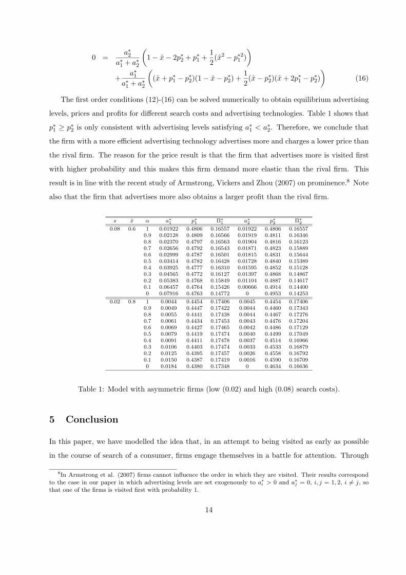
The first order conditions (12)-(16) can be solved numerically to obtain equilibrium advertising
levels, prices and profits for different search costs and advertising technologies. Table 1 shows that
p∗1 ≥ p∗2 is only consistent with advertising levels satisfying a∗1 < a∗2. Therefore, we conclude that
the firm with a more efficient advertising technology advertises more and charges a lower price than
the rival firm. The reason for the price result is that the firm that advertises more is visited first
with higher probability and this makes this firm demand more elastic than the rival firm. This
result is in line with the recent study of Armstrong, Vickers and Zhou (2007) on prominence.8 Note
also that the firm that advertises more also obtains a larger profit than the rival firm.
s x α a∗1 p∗1 Π∗1 a∗2 p∗2 Π∗20.08 0.6 1 0.01922 0.4806 0.16557 0.01922 0.4806 0.16557
0.9 0.02128 0.4809 0.16566 0.01919 0.4811 0.163460.8 0.02370 0.4797 0.16563 0.01904 0.4816 0.161230.7 0.02656 0.4792 0.16543 0.01871 0.4823 0.158890.6 0.02999 0.4787 0.16501 0.01815 0.4831 0.156440.5 0.03414 0.4782 0.16428 0.01728 0.4840 0.153890.4 0.03925 0.4777 0.16310 0.01595 0.4852 0.151280.3 0.04565 0.4772 0.16127 0.01397 0.4868 0.148670.2 0.05383 0.4768 0.15849 0.01104 0.4887 0.146170.1 0.06457 0.4764 0.15426 0.00666 0.4914 0.144000 0.07916 0.4763 0.14772 0 0.4953 0.14253
0.02 0.8 1 0.0044 0.4454 0.17406 0.0045 0.4454 0.174060.9 0.0049 0.4447 0.17422 0.0044 0.4460 0.173430.8 0.0055 0.4441 0.17438 0.0044 0.4467 0.172760.7 0.0061 0.4434 0.17453 0.0043 0.4476 0.172040.6 0.0069 0.4427 0.17465 0.0042 0.4486 0.171290.5 0.0079 0.4419 0.17474 0.0040 0.4499 0.170490.4 0.0091 0.4411 0.17478 0.0037 0.4514 0.169660.3 0.0106 0.4403 0.17474 0.0033 0.4533 0.168790.2 0.0125 0.4395 0.17457 0.0026 0.4558 0.167920.1 0.0150 0.4387 0.17419 0.0016 0.4590 0.167090 0.0184 0.4380 0.17348 0 0.4634 0.16636
Table 1: Model with asymmetric firms (low (0.02) and high (0.08) search costs).
5 Conclusion
In this paper, we have modelled the idea that, in an attempt to being visited as early as possible
in the course of search of a consumer, firms engage themselves in a battle for attention. Through
8In Armstrong et al. (2007) firms cannot influence the order in which they are visited. Their results correspondto the case in our paper in which advertising levels are set exogenously to a∗i > 0 and a∗j = 0, i, j = 1, 2, i 6= j, sothat one of the firms is visited first with probability 1.
14

investments in more and more appealing advertising, a firm can achieve a salient place in consumer
awareness so that consumers will visit this firm sooner when searching for a product they need.
Advertising is not a winner-takes-all contest in our setting: when a consumer does come to a firm
first, she can still decide to go to a different firm if she does not like the product of this particular
firm, or if she thinks it is too expensive.
We have found that prices and advertising levels are increasing in consumers’ search costs. Yet,
the effect on profits is ambiguous. If search costs are small to start with, then firms are better off if
search costs increase. Instead, when search costs are already high a further increase in search costs
lowers firm profits. In the latter case, getting the attention of a consumer becomes so important that
firms over-dissipate the rents generated by being visited earlier than rival firms. This highlights the
importance of looking at the interaction of advertising and search costs, rather than only looking
at search costs or advertising in isolation. We believe this to be a general phenomenon, that applies
beyond the scope of this particular model.
Another interesting finding is that firms with more efficient advertising technologies advertise
more, charge lower prices and obtain greater profits than less efficient rivals. Moreover, it is not clear
that firms benefit from more efficient advertising technologies. It turns out that lower advertising
costs may exacerbate an over-investment problem.
15

6 Appendix
Proof of Proposition 1
Using the expressions (14)-(4), we can compute
∂λi1
∂ai=
(n− 1) a∗
(ai + (n− 1) a∗)2(1− F (x + ∆))
· · ·∂λi
k
∂ai=
ai
ai + (n− k) a∗
k−1∑
`=1
− (n− `) a∗
(ai + (n− `) a∗)2
k−1∏
m6=`
(n−m) a∗
ai + (n−m) a∗
+(n− k) a∗
(ai + (n− k) a∗)2
k−1∏
`=1
(n− `) a∗
ai + (n− `) a∗
]F (x)k−1(1− F (x + ∆))
· · ·∂λi
n
∂ai=
n−1∑
`=1
− (n− `) a∗
(a + (n− `) a∗)2
n−1∏
m6=`
(n−m) a∗
a + (n−m) a∗
F (x)n−1(1− F (x + ∆))
In symmetric equilibrium we have
∂λi1
∂ai=
n− 1n2a∗
(1− F (x))
· · ·∂λi
k
∂ai=
1
n− k + 1
k−1∑
`=1
− (n− `)
(n− ` + 1)2 a∗
k−1∏
m6=`
n−m
n−m + 1
+n− i
(n− i + 1)2 a∗
k−1∏
`=1
n− `
n− ` + 1
]F (x)k−1 (1− F (x))
· · ·∂λi
n
∂ai=
n−1∑
`=1
− (n− `)
(n− ` + 1)2 a∗
n−1∏
m6=`
n−m
n−m + 1
F (x)n−1 (1− F (x)) .
Note thatk−1∏
`=1
n− `
n + 1− `=
n− 1n
· n− 2n− 1
· · · · · n + 1− k
n + 2− k=
n + 1− k
n.
16

This allows us to simplify some expressions, in particular:
∂λik
∂ai=
[1
n− k + 1
k−1∑
`=1
[ −1(n− ` + 1)2 a∗
(n + 1− k
n
)(n− ` + 1)
]
+n− k
(n− k + 1)na∗
]F (x)k−1 (1− F (x))
=1
na∗
[n− k
n− k + 1−
k−1∑
`=1
1(n− ` + 1)
]F (x)k−1 (1− F (x)) , for all k = 1, 2, ..., n.
Moreovern∑
k=1
λk(a∗, p∗) =1n
(1− F (x)n)
Using these derivations and the expression for R(p∗) in (5) above, the first order conditions in
(7) and (8) can be rewritten as:
p∗n∑
k=1
1na∗
(n− k
n− k + 1−
k−1∑
`=1
1(n− ` + 1)
)F (x)k−1 (1− F (x))− 1 = 0,
1− F (x)n
n+
∫ x
p∗F (ε)n−1f(ε)dε
+p∗(−f(x)
n
1− F (x)n
1− F (x)−
∫ x
p∗(n− 1)F (ε)n−2f(ε)2dε− F (p∗)n−1f(p∗) + F (x)n−1f(x)
)= 0.
Let us denote
Ck ≡ n− k
n− k + 1−
k−1∑
`=1
1n− ` + 1
.
Using the integration by parts rule,9 these equations can be simplified to:
p∗1
na∗(1− F (x))
n∑
k=1
CkF (x)k−1 − 1 = 0, (17)
1− F (p∗)n
n+ p∗
(−f(x)
n
1− F (x)n
1− F (x)+
∫ x
p∗F (ε)n−1f ′(ε)dε
)= 0. (18)
Consider equation (18). To study the existence of a solution in p∗, it is useful to rewrite it as
follows:1− F (p∗)n
np∗=
f(x)n
1− F (x)n
1− F (x)−
∫ x
p∗F (ε)n−1f ′(ε)dε. (19)
Note that the LHS of (19) is a positive-valued function that decreases monotonically in p∗. More-
over, when p∗ → 0 the LHS goes to ∞. The RHS, by contrast is monotonically increasing in p∗.
9R b
audv = uv|ba −
R b
avdu.
17

Therefore, a solution satisfying p∗ < x exists if and only if the following condition holds:
1− F (x)xf(x)
< 1 (20)
where x follows from (1). Using the definition of x above, it is straightforward to verify that the
condition in the proposition is equivalent to (20)
Consider now equation (17). Solving for a∗ we get:
a∗ =p∗
n(1− F (x))
n∑
k=1
Ck · F (x)k−1,
Note that
Ck − Ck−1 =
(n− k
n− k + 1−
k−1∑
`=1
1n− ` + 1
)−
(n− k + 1n− k + 2
−k−2∑
`=1
1n− ` + 1
)
=n− k
n− k + 1− 1
n− k + 2− n− k + 1
n− k + 2=
−1n− k + 1
.
We thus have
Ck = Ck−1 − 1n− k + 1
,
which implies that
Ck =n− 1
n−
k−1∑
`=1
1n− `
.
For the equilibrium advertising level we then have
a∗ =p∗
n(1− F (x))
n∑
k=1
[n− 1
n−
k−1∑
`=1
1n− `
]· F (x)k−1
=p∗
n(1− F (x))
[n− 1
n
n∑
k=1
F (x)k−1 −n∑
k=1
k−1∑
`=1
1n− `
· F (x)k−1
]
=p∗
n(1− F (x))
[n− 1
n
n∑
k=1
F (x)k−1 −n−1∑
`=1
(1
n− `
n∑
k=`+1
F (x)k−1
)]
=p∗
n(1− F (x))
[n− 1
n
n−1∑
k=0
F (x)k −n−1∑
`=1
(1
n− `
n−1∑
k=`
F (x)k
)],
18

which can be further simplified to
a∗ =p∗
n(1− F (x))
[n− 1
n· 1− F (x)n
1− F (x)−
n−1∑
`=1
(1
n− `
)F (x)` − F (x)n
1− F (x)
]
=p∗
n
[n− 1
n· (1− F (x)n)−
n−1∑
`=1
(1
n− `
)F (x)`
(1− F (x)n−`
)]
=p∗
n
[1− F (x)n −
n−1∑
k=0
F (x)k(1− F (x)n−k
)
n− k
].
¥
Proof of Proposition 2.
We build on the proof of Proposition 1. The equilibrium price is given by the solution of the
following equation:
1− F (p∗)n
np∗=
f(x)n
1− F (x)n
1− F (x)−
∫ x
p∗F (ε)n−1f ′(ε)dε. (21)
Notice that in this equation the effects of higher search costs are manifested only through
changes in x. Note also that the LHS of (21) decreases in p∗ and does not depend on x. Therefore
we only need to study how the RHS of this equation changes with x. From above, we know that the
RHS of (21) is monotonically increasing in p∗ so if the RHS increases in x, then the price decreases
as x goes up, and, since x and search costs s are inversely related, increases as s goes down.
Taking the derivative of the RHS of (21) with respect to x yields:[f ′(x)(1− F (x)n)− nF (x)n−1f2(x)
](1− F (x)) + f(x)2(1− F (x)n)
n(1− F (x))2− F (x)n−1f ′(x) (22)
At this point we can follow the steps in Anderson and Renault (1999), which reveals that the proof
of this result does not depend on whether the market is covered or not. For completeness, we
provide the last steps. The expression in (22) can be written as:[f ′(x)(1− F (x)) + f2(x)
](1− F (x)n)
n(1− F (x))
[1− F (x)n
1− F (x)− nF (x)n−1
](23)
The first term is positive because of log concavity of 1 − F (·). The second term is also positive
because it equals∑n−1
k=0
[F (x)k − F (x)n−1
]and F is a distribution function.
We now prove that advertising intensities also increase as search costs go up. For simplicity, we
rewrite a∗ as
a∗ =p∗An
,
19

with
A ≡ (1− F (x)n)−n−1∑
k=0
F (x)k(1− F (x)n−k
)
n− k.
We take the derivative of a∗ with respect to x. From (1), we immediately have that x is decreasing
in s. Hence, for a∗ to be increasing in s, we need it to be decreasing in x. We have:
∂a∗
∂x=
A
n
∂p∗
∂x+
p∗
n
∂A
∂x< 0,
From the discussion above we know that ∂p∗/∂x < 0. Therefore, if we show that ∂A/∂x < 0, the
results follows. Dropping subscripts, we have
∂A
∂x= −nFn−1f − Fn−1f −
n−1∑
k=1
kF k−1(1− Fn−k
)− (n− k) F kFn−k−1
n− kf
= −nFn−1f − Fn−1f −n−1∑
k=1
kF k−1(1− Fn−k
)
n− kf +
n−1∑
k=0
Fn−1f
= −Fn−1f −n−1∑
k=1
kF k−1(1− Fn−k
)
n− kf < 0.
¥
Proof of Proposition ??
Plugging our expression for a∗ into the profit function yields:
Πi(a∗, p∗) = p∗n∑
k=1
1n
F (x)k−1 (1− F (x)) + p∗∫ x
p∗F (ε)n−1 f(ε) dε
− p∗
n
((1− F (x)n)−
n−1∑
k=0
F (x)k(1− F (x)n−k
)
n− k
)
= p∗[∫ x
p∗F (ε)n−1 f(ε) dε +
1n
n−1∑
k=0
F (x)k(1− F (x)n−k
)
n− k
].
For ease of exposition, we will write equilibrium profits as
Πi(·) = p∗T (p∗, x),
with
T (p∗, x) ≡∫ x
p∗F (ε)n−1 f(ε) dε +
1n
n−1∑
k=0
F (x)k(1− F (x)n−k
)
n− k,
and p∗ is given by the solution to (10). Again, we take derivatives with respect to reservation utility
20

x. We have∂Π(·)∂x
=∂p∗
∂x
(T (·) + p∗
∂T (·)∂p∗
)+ p∗
∂T (·)∂x
.
where
∂p∗
∂x= −
[f ′(x)(1−F (x))+f2(x)](1−F (x)n)
n(1−F (x))
[1−F (x)n
1−F (x) − nF (x)n−1]
−nF (p∗)f(p∗)p∗−(1−F (p∗)n)np∗2 − F (p∗)n−1f ′(p∗)
,
∂T (·)∂p∗
= −F (p∗)n−1f(p∗),
and∂T (x)
∂x=
n−1∑
k=1
F (x)k−1(k − nF (x)n−k
)
n− kf(x).
To get the last derivative, we have first taken the case k = 0 outside of the summation. The
derivative of this term then exactly drops out against the derivative of the first term in T.
To prove (A), consider the case where search costs are very small: s → 0. Then x → 1, so
F (x) → 1. In this case, from Proposition 1 it is straightforward to verify that lims→0 p∗ > 0.
Moreover since limF→1(1− Fn)/(1− F ) = n, we have that
lims→0
∂p∗
∂x= 0.
Also
lims→0
T (·) = 1,
lims→0
∂T (·)∂p∗
< 0,
lims→0
∂T (·)∂x
= − (n− 1) f(1) < 0
Taken these terms together, this implies
lims→0
∂Π(·)∂x
= − (n− 1) f(1) lims→0
p∗ < 0.
Now consider the (B) case in which search costs are high s → s, match values are uniformly
distributed and two firms operate in the industry. In this case, the equilibrium of the model is
21

given by:
p∗ =12
(√2s− 2 +
√8− 4
√2s + 2s
),
a∗ =sp∗
2,
Π∗ =12p∗(1− p∗2 − s),
where s ranges from 0 to 1/8 in this case. It is straightforward to verify that Π∗ is a strictly concave
function reaching a maximum at s = 0.0115631. ¥
22

References
Alba, J. W., and A. Chattopadhyay (1986): “Salience Effects in Brand Recall,” Journal of
Marketing Research, 23(4), 363–369.
Anderson, S., and R. Renault (1999): “Pricing, Product Diversity, and Search Costs: a
Bertrand-Chamberlin-Diamond model,” RAND Journal of Economics, 30, 719–735.
Arbatskaya, M. (2007): “Ordered Search,” RAND Journal of Economics, p. forthcoming.
Armstrong, M., J. Vickers, and J. Zhou (2007): “Prominence and Consumer Search,” mimeo.
Bagwell, K. (2007): “The Economic Analysis of Advertising,” in Handbook of Industrial Organi-
zation, ed. by M. Armstrong, and R. Porter, Handbooks in Economics, chapter 2. North-Holland,
Amsterdam.
Benabou, R. (1993): “Search Market Equilibrium, Bilateral Heterogeneity, and Repeat Pur-
chases,” Journal of Economic Theory, 60, 140–158.
Bester, H., and E. Petrakis (1995): “Price Competition and Advertising in Oligopoly,” Euro-
pean Economic Review, 39(6), 1075–1088.
Burdett, K., and K. L. Judd (1983): “Equilibrium Price Dispersion,” Econometrica, 51, 955–
970.
Butters, G. (1977): “Equilibrium Distribution of Prices and Advertising,” Review of Economic
Studies, 44, 465–492.
Carlson, J., and P. R. McAfee (1983): “Discrete Equilibrium Price Dispersion,” Journal of
Political Economy, 91, 480–493.
Comanor, W., and T. Wilson (1974): Advertising and Market Power. Harvard University Press,
Cambridge, MA.
Galbraith, J. K. (1967): The New Industrial State. Houghton Mifflin, Boston.
Grossman, G., and C. Shapiro (1984): “Informative Advertising with Differentiated Products,”
Review of Economic Studies, 51, 63–82.
23

Hortacsu, A., and C. Syverson (2004): “Product Differentiation, Search Costs, And Competi-
tion in the Mutual Fund Industry: A Case Study of S&P 500 Index Funds,” Quarterly Journal
of Economics, 119(2), 403–456.
Janssen, M. C., and J. L. Moraga-Gonzalez (2004): “”Strategic Pricing, Consumer Search
and the Number of Firms,” Review of Economic Studies, 71, 1089–1118.
(2007): “On Mergers in Consumer Search Markets,” Tinbergen Institute Discussion Papers
07-054/1.
Janssen, M. C., J. L. Moraga-Gonzalez, and M. R. Wildenbeest (2005): “Truly costly
sequential search and oligopolistic pricing,” International Journal of Industrial Organization, 23,
451–466.
Kaldor, N. (1950): “The Economic Aspects of Advertising,” Review of Economic Studies, 18,
1–27.
PriceWaterhouseCoopers (2005): “Global Entertainment and Media Outlook: 2006-2010,”
Discussion paper.
Rauh, M. T. (2004): “Wage and price controls in the equilibrium sequential search model,”
European Economic Review, 48, 1287–1300.
(2007): “Nonstandard foundations of equilibrium search models,” Journal of Economic
Theory, 127, 518–529.
Reinganum, J. (1979): “A Simple Model of Equilibrium Price Dispersion,” Journal of Political
Economy, 87, 851–858.
Rob, R. (1985): “Equilibrium Price Distributions,” Review of Economic Studies, 52, 457–504.
Robert, J., and D. O. Stahl (1993): “Informative Price Advertising in a Sequential Search
Model,” Econometrica, 61, 657–686.
Schmalensee, R. (1976): “A Model of Promotional Competition in Oligopoly,” The Review of
Economic Studies, 43(3), 493–507.
Shapiro, C. (1980): “Advertising and Welfare: Comment,” Bell Journal of Economics, 11(2),
749–752.
24

Solow, R. (1967): “The New Industrial State or Son of Affluence,” Public Interest, 9, 100–108.
Stahl, D. (1994): “Oligopolistic Pricing and Advertising,” Journal of Economic Theory, 64, 162–
177.
Stahl, D. O. (1988): “Oligopolistic Pricing with Sequential Consumer Search,” American Eco-
nomic Review, 78, 189–201.
Tullock, G. (1980): “Efficient Rent Seeking,” in Toward a Theory of the Rent Seeking Society,
ed. by G. T. J.M. Buchanan, R. Tollison, pp. 224–232. Texas A&M Press.
25
Recommended