
CMPE750 CMPE750 -- ShaabanShaaban#1 Lec # 1 Spring 2015 1-27-2015
Advanced Computer ArchitectureAdvanced Computer ArchitectureCourse Goal:Understanding important emerging design techniques, machine structures, technology factors, evaluation methods that will determine the form of high-performance programmable processors and computing systems in 21st Century.
Important Factors:• Driving Force: Applications with diverse and increased computational demands even in
mainstream computing (multimedia etc.)• Techniques must be developed to overcome the major limitations of current computing
systems to meet such demands:– Instruction-Level Parallelism (ILP) limitations, Memory latency, IO performance.– Increased branch penalty/other stalls in deeply pipelined CPUs.– General-purpose processors as only homogeneous system computing resource.
• Increased density of VLSI logic (> seven billion transistors in 2014)Enabling Technology for many possible solutions: – Enables implementing more advanced architectural enhancements.– Enables chip-level Thread Level Parallelism:
• Simultaneous Multithreading (SMT)/Chip Multiprocessors (CMPs, AKA multi-core processors).
– Enables a high-level of chip-level system integration.• System On Chip (SOC) approach

CMPE750 CMPE750 -- ShaabanShaaban#2 Lec # 1 Spring 2015 1-27-2015
Course TopicsTopics we will cover include:• Overcoming inherent ILP & clock scaling limitations by exploiting
Thread-level Parallelism (TLP):– Support for Simultaneous Multithreading (SMT).
• Alpha EV8. Intel P4 Xeon and Core i7 (aka Hyper-Threading), IBM Power5.– Chip Multiprocessors (CMPs):
• The Hydra Project: An example CMP with Hardware Data/Thread Level Speculation (TLS) Support. IBM Power4, 5, 6 ….
• Instruction Fetch Bandwidth/Memory Latency Reduction: – Conventional & Block-based Trace Cache (Intel P4).
• Advanced Dynamic Branch Prediction Techniques.• Towards micro heterogeneous computing systems:
– Vector processing. Vector Intelligent RAM (VIRAM).– Digital Signal Processing (DSP), Media Processors.– Graphics Processor Units (GPUs).– Re-Configurable Computing and Processors.
• Virtual Memory Design/Implementation Issues.
• High Performance Storage: Redundant Arrays of Disks (RAID).

CMPE750 CMPE750 -- ShaabanShaaban#3 Lec # 1 Spring 2015 1-27-2015
Mainstream Computer System ComponentsMainstream Computer System Components
SDRAMPC100/PC133100-133MHZ64-128 bits wide2-way inteleaved~ 900 MBYTES/SEC
Double DateRate (DDR) SDRAMPC3200400MHZ (effective 200x2)64-128 bits wide4-way interleaved~3.2 GBYTES/SEC(second half 2002)
RAMbus DRAM (RDRAM)PC800, PC1060 400-533MHZ (DDR)16-32 bits wide channel~ 1.6 - 3.2 GBYTES/SEC
( per channel)
CPU
CachesFront Side Bus (FSB)
I/O Devices:
MemoryControllers
adapters
DisksDisplaysKeyboards
Networks
NICs
I/O BusesMemoryController
Examples: Alpha, AMD K7: EV6, 400MHZIntel PII, PIII: GTL+ 133MHZIntel P4 800MHZ
Example: PCI-X 133MHZPCI, 33-66MHZ32-64 bits wide133-1024 MBYTES/SEC
1000MHZ - 3.8 GHz (a multiple of system bus speed)Pipelined ( 7 - 30 stages )Superscalar (max ~ 4 instructions/cycle) single-threadedDynamically-Scheduled or VLIWDynamic and static branch prediction
L1
L2
L3
Memory Bus
Support for one or more CPUs
Fast EthernetGigabit EthernetATM, Token Ring ..
NorthBridge
SouthBridge
Chipset
Central Processing Unit (CPU):General Propose Processor (GPP)
With 2- 8 processor cores per chip

CMPE750 CMPE750 -- ShaabanShaaban#4 Lec # 1 Spring 2015 1-27-2015
Computing Engine Choices• General Purpose Processors (GPPs): Intended for general purpose computing
(desktops, servers, clusters..)• Application-Specific Processors (ASPs): Processors with ISAs and
architectural features tailored towards specific application domains– E.g Digital Signal Processors (DSPs), Network Processors (NPs), Media Processors,
Graphics Processing Units (GPUs), Vector Processors??? ...• Co-Processors: A hardware (hardwired) implementation of specific
algorithms with limited programming interface (augment GPPs or ASPs)• Configurable Hardware:
– Field Programmable Gate Arrays (FPGAs)– Configurable array of simple processing elements
• Application Specific Integrated Circuits (ASICs): A custom VLSI hardware solution for a specific computational task
• The choice of one or more depends on a number of factors including:- Type and complexity of computational algorithm
(general purpose vs. Specialized)- Desired level of flexibility - Performance requirements- Development cost - System cost- Power requirements - Real-time constrains

CMPE750 CMPE750 -- ShaabanShaaban#5 Lec # 1 Spring 2015 1-27-2015
Computing Engine Choices
General PurposeProcessors (GPPs):
Application-SpecificProcessors (ASPs)
Co-ProcessorsApplication Specific Integrated Circuits
(ASICs)
Configurable Hardware
E.g Digital Signal Processors (DSPs), Network Processors (NPs), Media Processors, Graphics Processing Units (GPUs)
- Type and complexity of computational algorithms(general purpose vs. Specialized)
- Desired level of flexibility - Performance- Development cost - System cost- Power requirements - Real-time constrains
Selection Factors:
Programmability /Flexibility
Specialization , Development cost/timePerformance/Chip Area/Watt (Computational Efficiency)
Processor = Programmable computing element that runs programs written using a pre-defined set of instructions (ISA)
ISA Requirements → Processor Design
Software Hardware

CMPE750 CMPE750 -- ShaabanShaaban#6 Lec # 1 Spring 2015 1-27-2015
Computer System ComponentsComputer System Components
CPU
CachesFront Side Bus (FSB)
I/O Devices:
MemoryControllers
adapters
Disks (RAID)DisplaysKeyboards
Networks
NICs
I/O BusesMemoryController
L1
L2
L3
Memory Bus
Conventional & Block-based Trace Cache.
Integrate MemoryController & a portionof main memory with CPU: Intelligent RAM
Integrated memory Controller: AMD Opetron
IBM Power5
Memory Latency Reduction:
Enhancing Computing Performance & Capabilities:
• Support for Simultaneous Multithreading (SMT): Intel HT.• VLIW & intelligent compiler techniques: Intel/HP EPIC IA-64.• More Advanced Branch Prediction Techniques.• Chip Multiprocessors (CMPs): The Hydra Project. IBM Power 4,5• Vector processing capability: Vector Intelligent RAM (VIRAM).
Or Multimedia ISA extension.• Digital Signal Processing (DSP) capability in system.• Re-Configurable Computing hardware capability in system.
SMTCMP
NorthBridge
SouthBridge
Chipset
Recent Trend:More system components integration(lowers cost, improves system performance)
System On Chip (SOC) approach

CMPE750 CMPE750 -- ShaabanShaaban#7 Lec # 1 Spring 2015 1-27-2015
CMPE550 ReviewCMPE550 Review• Recent Trends in Computer Design.• Computer Performance Measures.• Instruction Pipelining.• Dynamic Branch Prediction.• Instruction-Level Parallelism (ILP).• Loop-Level Parallelism (LLP).• Dynamic Pipeline Scheduling.• Multiple Instruction Issue (CPI < 1): Superscalar vs. VLIW• Dynamic Hardware-Based Speculation• Cache Design & Performance.• Basic Virtual memory Issues

CMPE750 CMPE750 -- ShaabanShaaban#8 Lec # 1 Spring 2015 1-27-2015
Trends in Computer DesignTrends in Computer Design• The cost/performance ratio of computing systems have seen a steady
decline due to advances in:– Integrated circuit technology: decreasing feature size, λ
• Clock rate improves roughly proportional to improvement in λ• Number of transistors improves proportional to λ2 (or faster).• Rate of clock speed improvement have decreased in recent years.
– Architectural improvements in CPU design.• Microprocessor-based systems directly reflect IC and architectural
improvement in terms of a yearly 35 to 55% improvement in performance.
• Assembly language has been mostly eliminated and replaced by other alternatives such as C or C++
• Standard operating Systems (UNIX, Windows) lowered the cost of introducing new architectures.
• Emergence of RISC architectures and RISC-core architectures.• Adoption of quantitative approaches to computer design based on
empirical performance observations.• Increased importance of exploiting thread-level parallelism (TLP) in
main-stream computing systems.Simultaneous Multithreading SMT/Chip Multiprocessor (CMP)Chip-level Thread-Level Parallelism (TLP)

CMPE750 CMPE750 -- ShaabanShaaban#9 Lec # 1 Spring 2015 1-27-2015
Processor Performance TrendsProcessor Performance Trends
Microprocessors
Minicomputers
Mainframes
Supercomputers
Year
0.1
1
10
100
1000
1965 1970 1975 1980 1985 1990 1995 2000
Mass-produced microprocessors a cost-effective high-performance replacement for custom-designed mainframe/minicomputer CPUs
Microprocessor: Single-chip VLSI-based processor

CMPE750 CMPE750 -- ShaabanShaaban#10 Lec # 1 Spring 2015 1-27-2015
Microprocessor Performance Microprocessor Performance 19871987--9797
0
200
400
600
800
1000
1200
87 88 89 90 91 92 93 94 95 96 97
DEC Alpha 21264/600
DEC Alpha 5/500
DEC Alpha 5/300
DEC Alpha 4/266IBM POWER 100
DEC AXP/500
HP 9000/750
Sun-4/260
IBMRS/6000
MIPS M/120
MIPS M
2000
Integer SPEC92 PerformanceInteger SPEC92 Performance
> 100x performance increase in the last decade

CMPE750 CMPE750 -- ShaabanShaaban#11 Lec # 1 Spring 2015 1-27-2015
Microprocessor Transistor Count Growth RateMicroprocessor Transistor Count Growth Rate
Intel 4004 (2300 transistors)
Currently > 7 Billion
Still holds today
Moore’s Law:Moore’s Law:2X transistors/ChipEvery 1.5-2 years(circa 1970)
~ 3,000,000x transistor density increase in the last 45 years
How to best exploit increased transistor count?• Keep increasing cache capacity/levels?• Multiple GPP cores?• Integrate other types of computing elements?

CMPE750 CMPE750 -- ShaabanShaaban#12 Lec # 1 Spring 2015 1-27-2015
Microprocessor Frequency TrendMicroprocessor Frequency Trend
Result:Deeper PipelinesLonger stallsHigher CPI(lowers effective performance per cycle)
1. Frequency used to double each generation2. Number of gates/clock reduce by 25%3. Leads to deeper pipelines with more stages
(e.g Intel Pentium 4E has 30+ pipeline stages)
Realty Check:Clock frequency scalingis slowing down!(Did silicone finally hit the wall?)
386486
Pentium(R)
Pentium Pro(R)
Pentium(R) IIMPC750
604+604
601, 603
21264S
2126421164A
2116421064A
21066
10
100
1,000
10,000
1987
1989
1991
1993
1995
1997
1999
2001
2003
2005
Mhz
1
10
100
Gat
e D
elay
s/ C
lock
IntelIBM Power PCDECGate delays/clock
Processor freq scales by 2X per
generation
Why?1- Power leakage2- Clock distribution delays
T = I x CPI x C
Possible Solutions?- Exploit Thread-Level Parallelism (TLP)
at the chip level (SMT/CMP)- Utilize/integrate more-specialized
computing elements other than GPPs
No longerthe case

CMPE750 CMPE750 -- ShaabanShaaban#13 Lec # 1 Spring 2015 1-27-2015
Tran
sist
ors
1,000
10,000
100,000
1,000,000
10,000,000
100,000,000
1970 1975 1980 1985 1990 1995 2000 2005
Bit-level parallelism Instruction-level Thread-level (?)
i4004
i8008i8080
i8086
i80286
i80386
R2000
Pentium
R10000
R3000
Parallelism in Microprocessor VLSI GenerationsParallelism in Microprocessor VLSI Generations
Simultaneous Multithreading SMT:e.g. Intel’s Hyper-threading
Chip-Multiprocessors (CMPs)e.g IBM Power 4, 5
Intel Pentium D, Core DuoAMD Athlon 64 X2
Dual Core OpteronSun UltraSparc T1 (Niagara)
Chip-LevelParallelProcessing
Even more importantdue to slowing clock rate increase
Multiple micro-operationsper cycle(multi-cycle non-pipelined)
Superscalar/VLIWCPI <1Single-issue
PipelinedCPI =1
Not PipelinedCPI >> 1
(ILP)
Single Thread
(TLP)
Improving microprocessor generation performance by exploiting more levels of parallelism
Thread-Level Parallelism (TLP)
AKA Operation-Level Parallelism

CMPE750 CMPE750 -- ShaabanShaaban#14 Lec # 1 Spring 2015 1-27-2015
Microprocessor Architecture TrendsMicroprocessor Architecture TrendsCISC Machines
instructions take variable times to complete
RISC Machines (microcode)simple instructions, optimized for speed
RISC Machines (pipelined)same individual instruction latency
greater throughput through instruction "overlap"
Superscalar Processorsmultiple instructions executing simultaneously
Multithreaded Processorsadditional HW resources (regs, PC, SP)each context gets processor for x cycles
VLIW"Superinstructions" grouped togetherdecreased HW control complexity
Single Chip Multiprocessorsduplicate entire processors
(tech soon due to Moore's Law)
SIMULTANEOUS MULTITHREADINGmultiple HW contexts (regs, PC, SP)each cycle, any context may execute
CMPs
(SMT)
SMT/CMPs e.g. IBM Power5,6,7 , Intel Pentium D, Sun Niagara - (UltraSparc T1)
Intel Nehalem (Core i7)
SingleThreaded
(e.g IBM Power 4/5, AMD X2, X3, X4, Intel Core 2)
e.g. Intel’s HyperThreading (P4)
(Single or Multi-Threaded)
General Purpose Processor (GPP)
Chip-Level TLP

CMPE750 CMPE750 -- ShaabanShaaban#15 Lec # 1 Spring 2015 1-27-2015
Computer Technology Trends:Computer Technology Trends:Evolutionary but Rapid ChangeEvolutionary but Rapid Change
• Processor:– 1.5-1.6 performance improvement every year; Over 100X performance in last
decade.
• Memory:– DRAM capacity: > 2x every 1.5 years; 1000X size in last decade.– Cost per bit: Improves about 25% or more per year.– Only 15-25% performance improvement per year.
• Disk:– Capacity: > 2X in size every 1.5 years.– Cost per bit: Improves about 60% per year.– 200X size in last decade.– Only 10% performance improvement per year, due to mechanical limitations.
• Expected State-of-the-art PC First Quarter 2015 :– Processor clock speed: ~ 4000 MegaHertz (4 Giga Hertz)– Memory capacity: > 16000 MegaByte (16 Giga Bytes)– Disk capacity: > 6000 GigaBytes (6 Tera Bytes)
Performance gap compared to CPU performance causes system performance bottlenecks
With 2-16 processor coreson a single chip

CMPE750 CMPE750 -- ShaabanShaaban#16 Lec # 1 Spring 2015 1-27-2015
Architectural ImprovementsArchitectural Improvements• Increased optimization, utilization and size of cache systems with
multiple levels (currently the most popular approach to utilize the increased number of available transistors) .
• Memory-latency hiding techniques.• Optimization of pipelined instruction execution.• Dynamic hardware-based pipeline scheduling.• Improved handling of pipeline hazards.• Improved hardware branch prediction techniques.• Exploiting Instruction-Level Parallelism (ILP) in terms of multiple-
instruction issue and multiple hardware functional units.• Inclusion of special instructions to handle multimedia applications.• High-speed system and memory bus designs to improve data transfer
rates and reduce latency.• Increased exploitation of Thread-Level Parallelism in terms of
Simultaneous Multithreading (SMT) and Chip Multiprocessors (CMPs)
Including Simultaneous Multithreading (SMT)

CMPE750 CMPE750 -- ShaabanShaaban#17 Lec # 1 Spring 2015 1-27-2015
Metrics of Computer PerformanceMetrics of Computer Performance
Compiler
Programming Language
Application
DatapathControl
Transistors Wires Pins
ISA
Function UnitsCycles per second (clock rate).
Megabytes per second.
Execution time: Target workload,SPEC95, SPEC2000, etc.
Each metric has a purpose, and each can be misused.
(millions) of Instructions per second – MIPS(millions) of (F.P.) operations per second – MFLOP/s
(Measures)

CMPE750 CMPE750 -- ShaabanShaaban#18 Lec # 1 Spring 2015 1-27-2015
CPU Execution Time: The CPU EquationCPU Execution Time: The CPU Equation• A program is comprised of a number of instructions executed , I
– Measured in: instructions/program
• The average instruction executed takes a number of cycles per instruction (CPI) to be completed. – Measured in: cycles/instruction, CPI
• CPU has a fixed clock cycle time C = 1/clock rate– Measured in: seconds/cycle
• CPU execution time is the product of the above three parameters as follows:
CPU time = Seconds = Instructions x Cycles x SecondsProgram Program Instruction Cycle
CPU time = Seconds = Instructions x Cycles x SecondsProgram Program Instruction Cycle
T = I x CPI x Cexecution Time
per program in secondsNumber of
instructions executedAverage CPI for program CPU Clock Cycle
(This equation is commonly known as the CPU performance equation)
Or Instructions Per Cycle (IPC):IPC= 1/CPI
Executed

CMPE750 CMPE750 -- ShaabanShaaban#19 Lec # 1 Spring 2015 1-27-2015
Factors Affecting CPU PerformanceFactors Affecting CPU PerformanceCPU time = Seconds = Instructions x Cycles x Seconds
Program Program Instruction Cycle
CPU time = Seconds = Instructions x Cycles x SecondsProgram Program Instruction Cycle
CPIIPC
Clock Cycle CInstructionCount I
Program
Compiler
Organization(Micro-Architecture)
Technology
Instruction SetArchitecture (ISA)
X
X
X
X
X
X
X X
X
T = I x CPI x C
VLSI

CMPE750 CMPE750 -- ShaabanShaaban#20 Lec # 1 Spring 2015 1-27-2015
Performance Enhancement Calculations:Performance Enhancement Calculations:Amdahl's LawAmdahl's Law
• The performance enhancement possible due to a given design improvement is limited by the amount that the improved feature is used
• Amdahl’s Law:Performance improvement or speedup due to enhancement E:
Execution Time without E Performance with ESpeedup(E) = -------------------------------------- = ---------------------------------
Execution Time with E Performance without E
– Suppose that enhancement E accelerates a fraction F of the execution time by a factor S and the remainder of the time is unaffected then:
Execution Time with E = ((1-F) + F/S) X Execution Time without E Hence speedup is given by:
Execution Time without E 1Speedup(E) = --------------------------------------------------------- = --------------------
((1 - F) + F/S) X Execution Time without E (1 - F) + F/SF (Fraction of execution time enhanced) refers to original execution time before the enhancement is applied
CMPE750 CMPE750 -- ShaabanShaaban#21 Lec # 1 Spring 2015 1-27-2015
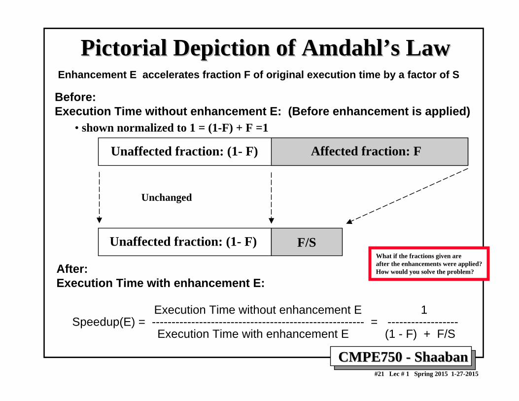
Pictorial Depiction of Amdahl’s LawPictorial Depiction of Amdahl’s Law
Before: Execution Time without enhancement E: (Before enhancement is applied)
After: Execution Time with enhancement E:
Enhancement E accelerates fraction F of original execution time by a factor of S
Unaffected fraction: (1- F) Affected fraction: F
Unaffected fraction: (1- F) F/S
Unchanged
Execution Time without enhancement E 1Speedup(E) = ------------------------------------------------------ = ------------------
Execution Time with enhancement E (1 - F) + F/S
• shown normalized to 1 = (1-F) + F =1
What if the fractions given areafter the enhancements were applied?How would you solve the problem?

CMPE750 CMPE750 -- ShaabanShaaban#22 Lec # 1 Spring 2015 1-27-2015
Extending Amdahl's Law To Multiple EnhancementsExtending Amdahl's Law To Multiple Enhancements
• Suppose that enhancement Ei accelerates a fraction Fi of the original execution time by a factor Si and the remainder of the time is unaffected then:
∑ ∑+−=
i ii
ii X
SFF
SpeedupTime Execution Original)1
Time Execution Original
)((
∑ ∑+−=
i ii
ii S
FFSpeedup
)( )1
1
(
Note: All fractions Fi refer to original execution time before theenhancements are applied.
.
Unaffected fraction
What if the fractions given areafter the enhancements were applied?How would you solve the problem?

CMPE750 CMPE750 -- ShaabanShaaban#23 Lec # 1 Spring 2015 1-27-2015
Amdahl's Law With Multiple Enhancements: Amdahl's Law With Multiple Enhancements: ExampleExample
• Three CPU or system performance enhancements are proposed with the following speedups and percentage of the code execution time affected:
Speedup1 = S1 = 10 Percentage1 = F1 = 20%Speedup2 = S2 = 15 Percentage1 = F2 = 15%Speedup3 = S3 = 30 Percentage1 = F3 = 10%
• While all three enhancements are in place in the new design, each enhancement affects a different portion of the code and only oneenhancement can be used at a time.
• What is the resulting overall speedup?
• Speedup = 1 / [(1 - .2 - .15 - .1) + .2/10 + .15/15 + .1/30)]= 1 / [ .55 + .0333 ] = 1 / .5833 = 1.71
∑ ∑+−=
i ii
ii S
FFSpeedup
)( )1
1
(

CMPE750 CMPE750 -- ShaabanShaaban#24 Lec # 1 Spring 2015 1-27-2015
Pictorial Depiction of ExamplePictorial Depiction of ExampleBefore: Execution Time with no enhancements: 1
After: Execution Time with enhancements: .55 + .02 + .01 + .00333 = .5833
Speedup = 1 / .5833 = 1.71
Note: All fractions (Fi , i = 1, 2, 3) refer to original execution time.
Unaffected, fraction: .55
Unchanged
Unaffected, fraction: .55 F1 = .2 F2 = .15 F3 = .1
S1 = 10 S2 = 15 S3 = 30
/ 10 / 30/ 15
What if the fractions given areafter the enhancements were applied?How would you solve the problem?

CMPE750 CMPE750 -- ShaabanShaaban#25 Lec # 1 Spring 2015 1-27-2015
“Reverse” Multiple Enhancements Amdahl's Law“Reverse” Multiple Enhancements Amdahl's Law• Multiple Enhancements Amdahl's Law assumes that the fractions given
refer to original execution time. • If for each enhancement Si the fraction Fi it affects is given as a fraction
of the resulting execution time after the enhancements were applied then:
• For the previous example assuming fractions given refer to resulting execution time after the enhancements were applied (not the original execution time), then:
Speedup = (1 - .2 - .15 - .1) + .2 x10 + .15 x15 + .1x30= .55 + 2 + 2.25 + 3= 7.8
TimeExecution ResultingTimeExecution Resulting)1 )(( XSFF ii ii iSpeedup
×+−= ∑∑
SFFSFFii ii i
ii ii iSpeedup ×+−=×+−
= ∑∑∑∑ )11
)1 ((Unaffected fraction
i.e as if resulting execution time is normalized to 1

CMPE750 CMPE750 -- ShaabanShaaban#26 Lec # 1 Spring 2015 1-27-2015
Instruction Pipelining ReviewInstruction Pipelining Review• Instruction pipelining is CPU implementation technique where multiple
operations on a number of instructions are overlapped.– Instruction pipelining exploits Instruction-Level Parallelism (ILP)
• An instruction execution pipeline involves a number of steps, where each step completes a part of an instruction. Each step is called a pipeline stage or a pipeline segment.
• The stages or steps are connected in a linear fashion: one stage to the next to form the pipeline -- instructions enter at one end and progress through the stages and exit at the other end.
• The time to move an instruction one step down the pipeline is is equal to the machine cycle and is determined by the stage with the longest processing delay.
• Pipelining increases the CPU instruction throughput: The number of instructions completed per cycle.
– Under ideal conditions (no stall cycles), instruction throughput is one instruction per machine cycle, or ideal CPI = 1
• Pipelining does not reduce the execution time of an individual instruction: The time needed to complete all processing steps of an instruction (also called instruction completion latency). – Minimum instruction latency = n cycles, where n is the number of pipeline
stages
The pipeline described here is called an in-order pipeline because instructions are processed or executed in the original program order
Pipelining may actually increase individual instruction latency
1 2 3 4 5
Or IPC = 1 T = I x CPI x C

CMPE750 CMPE750 -- ShaabanShaaban#27 Lec # 1 Spring 2015 1-27-2015
MIPS InMIPS In--Order SingleOrder Single--Issue Integer Pipeline Issue Integer Pipeline Ideal OperationIdeal Operation
Clock Number Time in clock cycles →Instruction Number 1 2 3 4 5 6 7 8 9
Instruction I IF ID EX MEM WBInstruction I+1 IF ID EX MEM WBInstruction I+2 IF ID EX MEM WBInstruction I+3 IF ID EX MEM WBInstruction I +4 IF ID EX MEM WB
Time to fill the pipeline
MIPS Pipeline Stages:
IF = Instruction FetchID = Instruction DecodeEX = ExecutionMEM = Memory AccessWB = Write Back
First instruction, ICompleted
Last instruction, I+4 completed
n= 5 pipeline stages Ideal CPI =1
Fill Cycles = number of stages -1
4 cycles = n -1
(No stall cycles)
Ideal pipeline operation without any stall cyclesIn-order = instructions executed in original program order
(or IPC =1)
(Classic 5-Stage)Pr
ogra
m O
rder
i.e execution in program order
CMPE750 CMPE750 -- ShaabanShaaban#28 Lec # 1 Spring 2015 1-27-2015
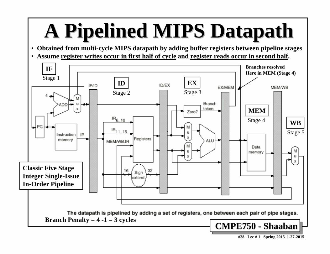
A Pipelined MIPS DatapathA Pipelined MIPS Datapath• Obtained from multi-cycle MIPS datapath by adding buffer registers between pipeline stages• Assume register writes occur in first half of cycle and register reads occur in second half.
IF
Classic Five Stage Integer Single-IssueIn-Order Pipeline
ID EX
MEM
WB
Branch Penalty = 4 -1 = 3 cycles
Branches resolvedHere in MEM (Stage 4)
Stage 1
Stage 2 Stage 3
Stage 4
Stage 5
CMPE750 CMPE750 -- ShaabanShaaban#29 Lec # 1 Spring 2015 1-27-2015
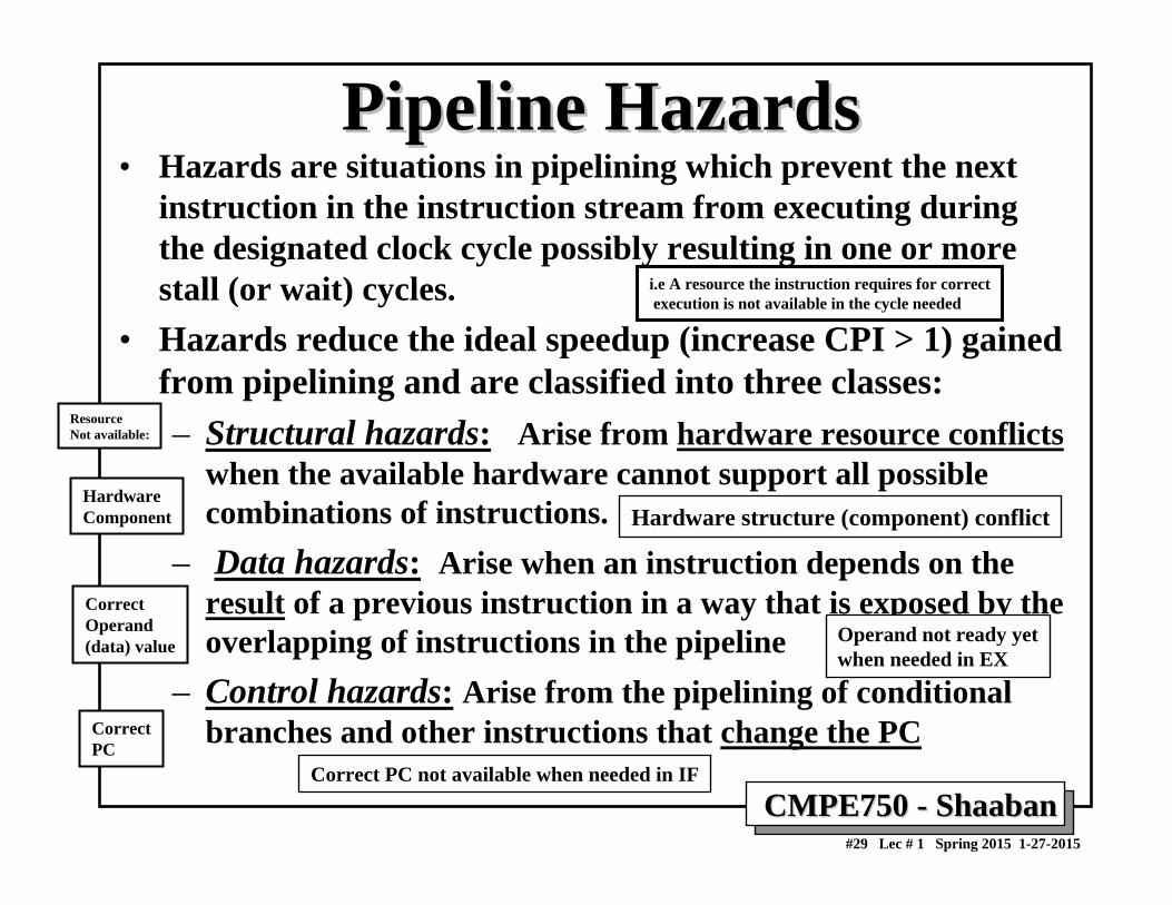
Pipeline HazardsPipeline Hazards• Hazards are situations in pipelining which prevent the next
instruction in the instruction stream from executing during the designated clock cycle possibly resulting in one or more stall (or wait) cycles.
• Hazards reduce the ideal speedup (increase CPI > 1) gained from pipelining and are classified into three classes:– Structural hazards: Arise from hardware resource conflicts
when the available hardware cannot support all possible combinations of instructions.
– Data hazards: Arise when an instruction depends on the result of a previous instruction in a way that is exposed by the overlapping of instructions in the pipeline
– Control hazards: Arise from the pipelining of conditional branches and other instructions that change the PC
i.e A resource the instruction requires for correctexecution is not available in the cycle needed
Resource Not available:
HardwareComponent
CorrectOperand(data) value
CorrectPC
Hardware structure (component) conflict
Operand not ready yetwhen needed in EX
Correct PC not available when needed in IF

CMPE750 CMPE750 -- ShaabanShaaban#30 Lec # 1 Spring 2015 1-27-2015
MIPS with MemoryMIPS with MemoryUnit Structural HazardsUnit Structural Hazards
One shared memory forinstructions and data

CMPE750 CMPE750 -- ShaabanShaaban#31 Lec # 1 Spring 2015 1-27-2015
Resolving A StructuralResolving A StructuralHazard with StallingHazard with Stalling
One shared memory forinstructions and data
Stall or waitCycle
CPI = 1 + stall clock cycles per instruction = 1 + fraction of loads and stores x 1
Instructions 1-3 above are assumed to be instructions other than loads/stores

CMPE750 CMPE750 -- ShaabanShaaban#32 Lec # 1 Spring 2015 1-27-2015
Data HazardsData Hazards• Data hazards occur when the pipeline changes the order of
read/write accesses to instruction operands in such a way that the resulting access order differs from the original sequential instruction operand access order of the unpipelined machine resulting in incorrect execution.
• Data hazards may require one or more instructions to be stalled to ensure correct execution.
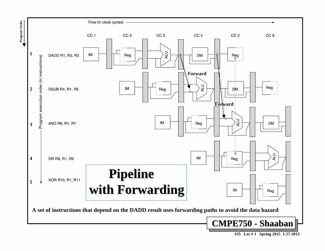
• Example:DADD R1, R2, R3DSUB R4, R1, R5AND R6, R1, R7OR R8,R1,R9XOR R10, R1, R11
– All the instructions after DADD use the result of the DADD instruction– DSUB, AND instructions need to be stalled for correct execution.
12345
Arrows represent data dependenciesbetween instructions
Instructions that have no dependencies among them are said to be parallel or independent
A high degree of Instruction-Level Parallelism (ILP)is present in a given code sequence if it has a largenumber of parallel instructions
i.e Correct operand data not ready yet when needed in EX cycle
CPI = 1 + stall clock cycles per instruction
Producer of Result
Consumers of Result

CMPE750 CMPE750 -- ShaabanShaaban#33 Lec # 1 Spring 2015 1-27-2015
Figure A.6 The use of the result of the DADD instruction in the next three instructionscauses a hazard, since the register is not written until after those instructions read it.
Data Data Hazard ExampleHazard Example
1
2
3
4
5
Two stall cycles are needed here(to prevent data hazard)
Prog
ram
Ord
er

CMPE750 CMPE750 -- ShaabanShaaban#34 Lec # 1 Spring 2015 1-27-2015
Minimizing Data hazard Stalls by Minimizing Data hazard Stalls by ForwardingForwarding• Data forwarding is a hardware-based technique (also called
register bypassing or short-circuiting) used to eliminate or minimize data hazard stalls.
• Using forwarding hardware, the result of an instruction is copied directly from where it is produced (ALU, memory read port etc.), to where subsequent instructions need it (ALU input register, memory write port etc.)
• For example, in the MIPS integer pipeline with forwarding:– The ALU result from the EX/MEM register may be forwarded or fed
back to the ALU input latches as needed instead of the registeroperand value read in the ID stage.
– Similarly, the Data Memory Unit result from the MEM/WB register may be fed back to the ALU input latches as needed .
– If the forwarding hardware detects that a previous ALU operation is to write the register corresponding to a source for the current ALUoperation, control logic selects the forwarded result as the ALU input rather than the value read from the register file.
CMPE750 CMPE750 -- ShaabanShaaban#35 Lec # 1 Spring 2015 1-27-2015
PipelinePipelinewith Forwardingwith Forwarding
A set of instructions that depend on the DADD result uses forwarding paths to avoid the data hazard
Forward
Forward
1
2
3
4
5
Prog
ram
Ord
er

CMPE750 CMPE750 -- ShaabanShaaban#36 Lec # 1 Spring 2015 1-27-2015
Data Hazard/Dependence ClassificationData Hazard/Dependence ClassificationI (Write)
SharedOperand
J (Read)
Read after Write (RAW)if data dependence is violated
I (Read)
SharedOperand
J (Write)Write after Read (WAR)if antidependence is violated
I (Read)
SharedOperand
J (Read)
Read after Read (RAR) not a hazard
I (Write)
SharedOperand
J (Write)Write after Write (WAW)if output dependence is violated
A name dependence:output dependence
A name dependence:antidependence
I....
J
ProgramOrder
No dependence
True Data Dependence
Or name
Or name

CMPE750 CMPE750 -- ShaabanShaaban#37 Lec # 1 Spring 2015 1-27-2015
Control HazardsControl Hazards• When a conditional branch is executed it may change the PC and,
without any special measures, leads to stalling the pipeline for a number of cycles until the branch condition is known (branch is resolved).– Otherwise the PC may not be correct when needed in IF
• In current MIPS pipeline, the conditional branch is resolved in stage 4 (MEM stage) resulting in three stall cycles as shown below:
Branch instruction IF ID EX MEM WBBranch successor stall stall stall IF ID EX MEM WBBranch successor + 1 IF ID EX MEM WB Branch successor + 2 IF ID EX MEMBranch successor + 3 IF ID EXBranch successor + 4 IF IDBranch successor + 5 IF
Assuming we stall or flush the pipeline on a branch instruction: Three clock cycles are wasted for every branch for current MIPS pipeline
Branch Penalty = stage number where branch is resolved - 1 here Branch Penalty = 4 - 1 = 3 Cycles
3 stall cycles
Branch Penalty Correct PC available here(end of MEM cycle or stage)
i.e Correct PC is not available when needed in IF
CMPE750 CMPE750 -- ShaabanShaaban#38 Lec # 1 Spring 2015 1-27-2015
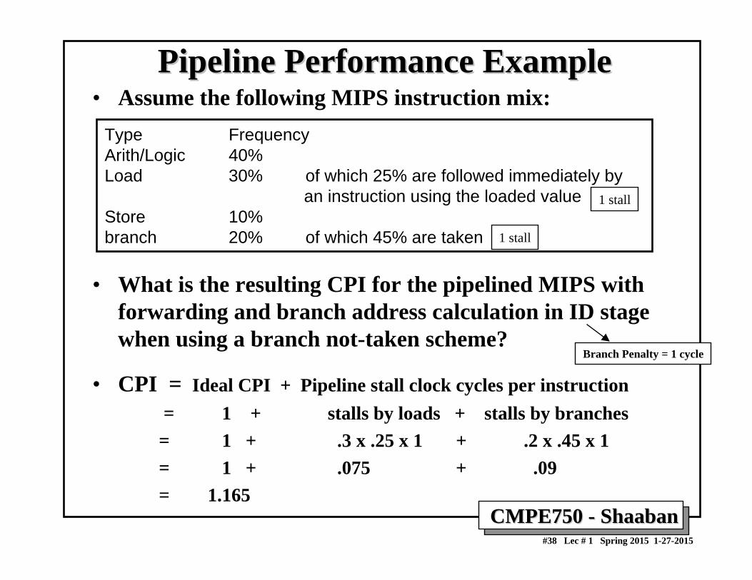
Pipeline Performance ExamplePipeline Performance Example• Assume the following MIPS instruction mix:
• What is the resulting CPI for the pipelined MIPS with forwarding and branch address calculation in ID stage when using a branch not-taken scheme?
• CPI = Ideal CPI + Pipeline stall clock cycles per instruction= 1 + stalls by loads + stalls by branches= 1 + .3 x .25 x 1 + .2 x .45 x 1= 1 + .075 + .09 = 1.165
Type FrequencyArith/Logic 40%Load 30% of which 25% are followed immediately by
an instruction using the loaded value Store 10%branch 20% of which 45% are taken
Branch Penalty = 1 cycle
1 stall
1 stall

CMPE750 CMPE750 -- ShaabanShaaban#39 Lec # 1 Spring 2015 1-27-2015
Pipelining and Exploiting Pipelining and Exploiting InstructionInstruction--Level Parallelism (ILP)Level Parallelism (ILP)
• Instruction-Level Parallelism (ILP) exists when instructions in a sequence are independent and thus can be executed in parallel by overlapping.
– Pipelining increases performance by overlapping the execution ofindependent instructions and thus exploits ILP in the code.
• Preventing instruction dependency violations (hazards) may result in stall cycles in a pipelined CPU increasing its CPI (reducing performance).
– The CPI of a real-life pipeline is given by (assuming ideal memory):
Pipeline CPI = Ideal Pipeline CPI + Structural Stalls + RAW Stalls+ WAR Stalls + WAW Stalls + Control Stalls
• Programs that have more ILP (fewer dependencies) tend to perform better on pipelined CPUs.– More ILP mean fewer instruction dependencies and thus fewer stall
cycles needed to prevent instruction dependency violations
In Fourth Edition Chapter 2.1(In Third Edition Chapter 3.1)
(without stalling)
T = I x CPI x C
i.e hazards
Dependency Violation = Hazard
i.e instruction throughput
i.e non-ideal

CMPE750 CMPE750 -- ShaabanShaaban#40 Lec # 1 Spring 2015 1-27-2015
Basic Instruction Block• A basic instruction block is a straight-line code sequence with no
branches in, except at the entry point, and no branches out except at the exit point of the sequence. – Example: Body of a loop.
• The amount of instruction-level parallelism (ILP) in a basic block is limited by instruction dependence present and size of the basic block.
• In typical integer code, dynamic branch frequency is about 15% (resulting average basic block size of about 7 instructions).
• Any static technique that increases the average size of basic blocks which increases the amount of exposed ILP in the code and provide more instructions for static pipeline scheduling by the compiler possibly eliminating more stall cycles and thus improves pipelined CPU performance.– Loop unrolling is one such technique that we examine next
Start of Basic Block
End of Basic Block
Static = At compilation time Dynamic = At run time
: :: :
Branch In
Branch (out)
Basic Block
In Fourth Edition Chapter 2.1 (In Third Edition Chapter 3.1)

CMPE750 CMPE750 -- ShaabanShaaban#41 Lec # 1 Spring 2015 1-27-2015
ABDH
EJ
...
I
...
K
...
...CFL
GN...
...
M
O
...
Static ProgramOrder
Average Basic Block Size = 5-7 instructions
Program Control Flow Graph (CFG)
NT = Branch Not TakenT = Branch Taken
• A-O = Basic Blocks terminating with conditional branches
• The outcomes of branches determine the basic block dynamic execution sequence or trace
If all three branches are takenthe execution trace will be basic blocks: ACGO
Basic Blocks/Dynamic Execution Sequence (Trace) Example
Trace: Dynamic Sequence of basic blocks executed
Type of branches in this example:“If-Then-Else” branches (not loops)

CMPE750 CMPE750 -- ShaabanShaaban#42 Lec # 1 Spring 2015 1-27-2015
Increasing InstructionIncreasing Instruction--Level Parallelism (ILP)Level Parallelism (ILP)• A common way to increase parallelism among instructions is to
exploit parallelism among iterations of a loop – (i.e Loop Level Parallelism, LLP).
• This is accomplished by unrolling the loop either statically by the compiler, or dynamically by hardware, which increases the size of the basic block present. This resulting larger basic block provides more instructions that can be scheduled or re-ordered by the compiler to eliminate more stall cycles.
• In this loop every iteration can overlap with any other iteration. Overlap within each iteration is minimal.
for (i=1; i<=1000; i=i+1;)x[i] = x[i] + y[i];
• In vector machines, utilizing vector instructions is an important alternative to exploit loop-level parallelism,
• Vector instructions operate on a number of data items. The above loop would require just four such instructions.
4 vector instructions:Load Vector XLoad Vector YAdd Vector X, X, YStore Vector X
Or Data Parallelism in a loop
(potentially)
i.e independent or parallel loop iterations
Example:
Independent (parallel) loop iterations:A result of high degree of data parallelism
In Fourth Edition Chapter 2.2 (In Third Edition Chapter 4.1)

CMPE750 CMPE750 -- ShaabanShaaban#43 Lec # 1 Spring 2015 1-27-2015
MIPS Loop Unrolling ExampleMIPS Loop Unrolling Example• For the loop:
for (i=1000; i>0; i=i-1)x[i] = x[i] + s;
The straightforward MIPS assembly code is given by:
Loop: L.D F0, 0 (R1) ;F0=array elementADD.D F4, F0, F2 ;add scalar in F2 (constant)S.D F4, 0(R1) ;store resultDADDUI R1, R1, # -8 ;decrement pointer 8 bytesBNE R1, R2,Loop ;branch R1!=R2
R1 is initially the address of the element with highest address.8(R2) is the address of the last element to operate on. Basic block size = 5 instructions
X[ ] array of double-precision floating-point numbers (8-bytes each)
X[1000]X[999]
X[1]
R1 initially
points here
R2 points here
First element to compute
High Memory
Low Memory
R2 +8 points here
.
.
.
.
R1 -8 points here
Last element to compute
Note:IndependentLoop Iterations
Initial value of R1 = R2 + 8000
Prog
ram
Ord
er
S
In Fourth Edition Chapter 2.2 (In Third Edition Chapter 4.1)

CMPE750 CMPE750 -- ShaabanShaaban#44 Lec # 1 Spring 2015 1-27-2015
MIPS FP Latency AssumptionsMIPS FP Latency Assumptions
• All FP units assumed to be pipelined.• The following FP operations latencies are used:
Instruction Producing Result
FP ALU Op
FP ALU Op
Load Double
Load Double
Instruction Using Result
Another FP ALU Op
Store Double
FP ALU Op
Store Double
Latency InClock Cycles
3
2
1
0
(or Number of Stall Cycles)
For Loop Unrolling Example
i.e 4 execution(EX) cycles for FP instructions
i.e followed immediately by ..
- Branch resolved in decode stage, Branch penalty = 1 cycle - Full forwarding is used- Single Branch delay Slot - Potential structural hazards ignored
Other Assumptions:
In Fourth Edition Chapter 2.2 (In Third Edition Chapter 4.1)

CMPE750 CMPE750 -- ShaabanShaaban#45 Lec # 1 Spring 2015 1-27-2015
Loop Unrolling Example (continued)Loop Unrolling Example (continued)• This loop code is executed on the MIPS pipeline as follows:
(Branch resolved in decode stage, Branch penalty = 1 cycle, Full forwarding is used)
Scheduled with single delayed branch slot:
Loop: L.D F0, 0(R1)DADDUI R1, R1, # -8ADD.D F4, F0, F2stallBNE R1,R2, LoopS.D F4,8(R1)
6 cycles per iteration
No schedulingClock cycle
Loop: L.D F0, 0(R1) 1stall 2ADD.D F4, F0, F2 3stall 4stall 5S.D F4, 0 (R1) 6DADDUI R1, R1, # -8 7stall 8BNE R1,R2, Loop 9stall 10
10 cycles per iteration 10/6 = 1.7 times faster
• Ignoring Pipeline Fill Cycles• No Structural Hazards
Due toresolvingbranchin ID S.D in branch delay slot
(Resulting stalls shown)
(Resulting stalls shown)Cycle123456
Prog
ram
Ord
er
In Fourth Edition Chapter 2.2 (In Third Edition Chapter 4.1)

CMPE750 CMPE750 -- ShaabanShaaban#46 Lec # 1 Spring 2015 1-27-2015
Loop Unrolling Example (continued)Loop Unrolling Example (continued)
• The resulting loop code when four copies of the loop body are unrolled without reuse of registers.
• The size of the basic block increased from 5 instructions in the original loop to 14 instructions.
No schedulingLoop: L.D F0, 0(R1)
Stall
ADD.D F4, F0, F2StallStall
SD F4,0 (R1) ; drop DADDUI & BNE
LD F6, -8(R1)Stall
ADDD F8, F6, F2StallStall
SD F8, -8 (R1), ; drop DADDUI & BNE
LD F10, -16(R1)Stall
ADDD F12, F10, F2StallStall
SD F12, -16 (R1) ; drop DADDUI & BNE
LD F14, -24 (R1)Stall
ADDD F16, F14, F2StallStall
SD F16, -24(R1)DADDUI R1, R1, # -32Stall
BNE R1, R2, LoopStall
Three branches and three decrements of R1 are eliminated.
Load and store addresses arechanged to allow DADDUI instructions to be merged.
The unrolled loop runs in 28 cycles assuming each L.D has 1 stall cycle, each ADD.D has 2 stall cycles, the DADDUI 1 stall, the branch 1 stall cycle, or 28/4 = 7 cycles to produce each of the four elements.
12
3456789101112131415161718
19202122232425262728
Cycle
i.e. unrolled four timesNote use of different registers for each iteration (register renaming)
RegisterRenamingUsed
i.e 7 cycles for each original iteration
Loop unrolled 4 times
1
2
3
4
Iteration
(Resulting stalls shown)
New Basic Block Size = 14 Instructions
Performance:
In Fourth Edition Chapter 2.2 (In Third Edition Chapter 4.1)

CMPE750 CMPE750 -- ShaabanShaaban#47 Lec # 1 Spring 2015 1-27-2015
Loop Unrolling Example (continued)Loop Unrolling Example (continued)
When scheduled for pipeline
Loop: L.D F0, 0(R1)L.D F6,-8 (R1)L.D F10, -16(R1)L.D F14, -24(R1)ADD.D F4, F0, F2ADD.D F8, F6, F2ADD.D F12, F10, F2ADD.D F16, F14, F2S.D F4, 0(R1)S.D F8, -8(R1)DADDUI R1, R1,# -32S.D F12, 16(R1),F12BNE R1,R2, LoopS.D F16, 8(R1), F16 ;8-32 = -24
The execution time of the loophas dropped to 14 cycles, or 14/4 = 3.5 clock cycles per element
compared to 7 before schedulingand 6 when scheduled but unrolled.
Speedup = 6/3.5 = 1.7
Unrolling the loop exposed more computations that can be scheduled to minimize stalls by increasing the size of the basic block from 5 instructionsin the original loop to 14 instructionsin the unrolled loop.
Larger Basic Block More ILP
i.e 3.5 cycles for each original iteration
In branch delay slot
i.e more ILPexposed
Exposed
Note: No stalls
Prog
ram
Ord
er
In Fourth Edition Chapter 2.2 (In Third Edition Chapter 4.1)
Offset = 16 - 32 = -16

CMPE750 CMPE750 -- ShaabanShaaban#48 Lec # 1 Spring 2015 1-27-2015
LoopLoop--Level Parallelism (LLP) AnalysisLevel Parallelism (LLP) Analysis• Loop-Level Parallelism (LLP) analysis focuses on whether data accesses in later
iterations of a loop are data dependent on data values produced in earlier iterations and possibly making loop iterations independent (parallel).
e.g. in for (i=1; i<=1000; i++)x[i] = x[i] + s;
the computation in each iteration is independent of the previous iterations and the loop is thus parallel. The use of X[i] twice is within a single iteration.
⇒ Thus loop iterations are parallel (or independent from each other).
• Loop-carried Data Dependence: A data dependence between different loop iterations (data produced in an earlier iteration used in a later one).
• Not Loop-carried Data Dependence: Data dependence within the same loop iteration.
• LLP analysis is important in software optimizations such as loop unrolling since it usually requires loop iterations to be independent (and in vector processing).
• LLP analysis is normally done at the source code level or close to it since assembly language and target machine code generation introduces loop-carried name dependence in the registers used in the loop.
– Instruction level parallelism (ILP) analysis, on the other hand, is usually done when instructions are generated by the compiler.
S1(Body of Loop)
S1 S1 S1 S1
Dependency Graph
Iteration # 1 2 3 ….. 1000
…Usually: Data Parallelism → LLP
Classification of Date Dependencies in Loops:
4th Edition: Appendix G.1-G.2 (3rd Edition: Chapter 4.4)
1
2
CMPE750 CMPE750 -- ShaabanShaaban#49 Lec # 1 Spring 2015 1-27-2015
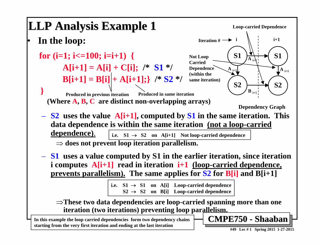
LLP Analysis Example 1LLP Analysis Example 1• In the loop:
for (i=1; i<=100; i=i+1) {A[i+1] = A[i] + C[i]; /* S1 */B[i+1] = B[i] + A[i+1];} /* S2 */
}(Where A, B, C are distinct non-overlapping arrays)
– S2 uses the value A[i+1], computed by S1 in the same iteration. This data dependence is within the same iteration (not a loop-carried dependence).
⇒ does not prevent loop iteration parallelism.
– S1 uses a value computed by S1 in the earlier iteration, since iteration i computes A[i+1] read in iteration i+1 (loop-carried dependence, prevents parallelism). The same applies for S2 for B[i] and B[i+1]
⇒These two data dependencies are loop-carried spanning more than one iteration (two iterations) preventing loop parallelism.
S1
S2
S1
S2
Dependency Graph
Iteration # i i+1
A i+1
B i+1
A i+1 A i+1
Not LoopCarriedDependence(within thesame iteration)
Loop-carried Dependence
In this example the loop carried dependencies form two dependency chains starting from the very first iteration and ending at the last iteration
i.e. S1 → S2 on A[i+1] Not loop-carried dependence
i.e. S1 → S1 on A[i] Loop-carried dependenceS2 → S2 on B[i] Loop-carried dependence
Produced in previous iteration Produced in same iteration

CMPE750 CMPE750 -- ShaabanShaaban#50 Lec # 1 Spring 2015 1-27-2015
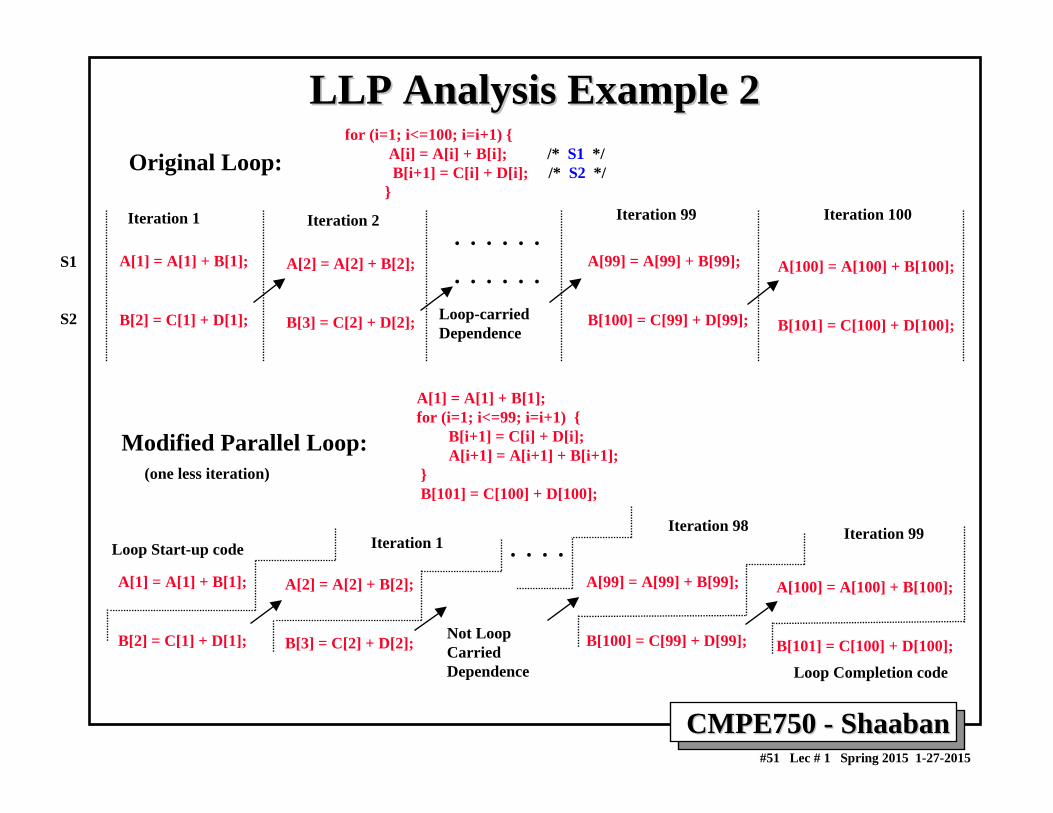
LLP Analysis Example 2LLP Analysis Example 2• In the loop:
for (i=1; i<=100; i=i+1) {A[i] = A[i] + B[i]; /* S1 */B[i+1] = C[i] + D[i]; /* S2 */
}– S1 uses the value B[i] computed by S2 in the previous iteration (loop-
carried dependence)– This dependence is not circular:
• S1 depends on S2 but S2 does not depend on S1.– Can be made parallel by replacing the code with the following:
A[1] = A[1] + B[1];for (i=1; i<=99; i=i+1) {
B[i+1] = C[i] + D[i];A[i+1] = A[i+1] + B[i+1];
}B[101] = C[100] + D[100];
Loop Start-up code
Loop Completion code
Parallel loop iterations(data parallelism in computationexposed in loop code)
S1
S2
S1
S2
Dependency Graph
Iteration # i i+1
B i+1
Loop-carried Dependence
i.e. S2 → S1 on B[i] Loop-carried dependence
i.e. loop
4th Edition: Appendix G.2 (3rd Edition: Chapter 4.4)
And does not form a data dependence chain
CMPE750 CMPE750 -- ShaabanShaaban#51 Lec # 1 Spring 2015 1-27-2015
LLP Analysis Example 2LLP Analysis Example 2Original Loop:
A[100] = A[100] + B[100];
B[101] = C[100] + D[100];
A[1] = A[1] + B[1];
B[2] = C[1] + D[1];
A[2] = A[2] + B[2];
B[3] = C[2] + D[2];
A[99] = A[99] + B[99];
B[100] = C[99] + D[99];
A[100] = A[100] + B[100];
B[101] = C[100] + D[100];
A[1] = A[1] + B[1];
B[2] = C[1] + D[1];
A[2] = A[2] + B[2];
B[3] = C[2] + D[2];
A[99] = A[99] + B[99];
B[100] = C[99] + D[99];
for (i=1; i<=100; i=i+1) {A[i] = A[i] + B[i]; /* S1 */B[i+1] = C[i] + D[i]; /* S2 */
}
A[1] = A[1] + B[1];for (i=1; i<=99; i=i+1) {
B[i+1] = C[i] + D[i];A[i+1] = A[i+1] + B[i+1];
}B[101] = C[100] + D[100];
Modified Parallel Loop:
Iteration 1 Iteration 2 Iteration 100Iteration 99
Loop-carried Dependence
Loop Start-up code
Loop Completion code
Iteration 1Iteration 98 Iteration 99
Not LoopCarried Dependence
. . . . . .
. . . . . .
. . . .
S1
S2
(one less iteration)

CMPE750 CMPE750 -- ShaabanShaaban#52 Lec # 1 Spring 2015 1-27-2015
Reduction of Data Hazards Stalls Reduction of Data Hazards Stalls with Dynamic Schedulingwith Dynamic Scheduling
• So far we have dealt with data hazards in instruction pipelines by:
– Result forwarding (register bypassing) to reduce or eliminate stalls needed to prevent RAW hazards as a result of true data dependence.
– Hazard detection hardware to stall the pipeline starting with the instruction that uses the result.
– Compiler-based static pipeline scheduling to separate the dependent instructions minimizing actual hazard-prevention stalls in scheduled code.
• Loop unrolling to increase basic block size: More ILP exposed.
• Dynamic scheduling: (out-of-order execution)– Uses a hardware-based mechanism to reorder or rearrange instruction
execution order to reduce stalls dynamically at runtime.• Better dynamic exploitation of instruction-level parallelism (ILP).
– Enables handling some cases where instruction dependencies are unknown at compile time (ambiguous dependencies).
– Similar to the other pipeline optimizations above, a dynamically scheduled processor cannot remove true data dependencies, but tries to avoid or reduce stalling.
i.e Start of instruction execution is not in program order
Why?
Fourth Edition: Appendix A.7, Chapter 2.4, 2.5(Third Edition: Appendix A.8, Chapter 3.2, 3.3)
i.e forward + stall (if needed)

CMPE750 CMPE750 -- ShaabanShaaban#53 Lec # 1 Spring 2015 1-27-2015
Dynamic Pipeline Scheduling:Dynamic Pipeline Scheduling: The ConceptThe Concept• Dynamic pipeline scheduling overcomes the limitations of in-order
pipelined execution by allowing out-of-order instruction execution.
• Instruction are allowed to start executing out-of-order as soon as their operands are available.
• Better dynamic exploitation of instruction-level parallelism (ILP).
Example:
• This implies allowing out-of-order instruction commit (completion).• May lead to imprecise exceptions if an instruction issued earlier
raises an exception. – This is similar to pipelines with multi-cycle floating point units.
In the case of in-order pipelined execution SUB.D must wait for DIV.D to complete which stalled ADD.D before starting executionIn out-of-order execution SUBD can start as soon as the values of its operands F8, F14 are available.
DIV.D F0, F2, F4ADD.D F10, F0, F8SUB.D F12, F8, F14
True DataDependency
Does not depend on DIV.D or ADD.D
(Out-of-order execution)
1
2
3
DependencyGraph
1
2
3
i.e Start of instruction execution is not in program order
Order = Program Instruction Order
Program Order
In Fourth Edition: Appendix A.7, Chapter 2.4(In Third Edition: Appendix A.8, Chapter 3.2)

CMPE750 CMPE750 -- ShaabanShaaban#54 Lec # 1 Spring 2015 1-27-2015
Dynamic Scheduling: Dynamic Scheduling: The Tomasulo AlgorithmThe Tomasulo Algorithm
• Developed at IBM and first implemented in IBM’s 360/91 mainframe in 1966, about 3 years after the debut of the scoreboard in the CDC 6600.
• Dynamically schedule the pipeline in hardware to reduce stalls.
• Differences between IBM 360 & CDC 6600 ISA.– IBM has only 2 register specifiers/instr vs. 3 in CDC 6600.– IBM has 4 FP registers vs. 8 in CDC 6600.
• Current CPU architectures that can be considered descendants of the IBM 360/91 which implement and utilize a variation of the Tomasulo Algorithm include:
RISC CPUs: Alpha 21264, HP 8600, MIPS R12000, PowerPC G4RISC-core x86 CPUs: AMD Athlon, Pentium III, 4, Xeon ….
In Fourth Edition: Chapter 2.4 (In Third Edition: Chapter 3.2)A Tomasulo simulator: http://www.ecs.umass.edu/ece/koren/architecture/Tomasulo1/tomasulo.htm

CMPE750 CMPE750 -- ShaabanShaaban#55 Lec # 1 Spring 2015 1-27-2015
Dynamic Scheduling: The Tomasulo ApproachDynamic Scheduling: The Tomasulo Approach
The basic structure of a MIPS floating-point unit using Tomasulo’s algorithm
(Instruction Fetch)
(IQ)
Pipelined FP units are used here
Instructions to Issue(in program order)
In Fourth Edition: Chapter 2.4(In Third Edition: Chapter 3.2)

CMPE750 CMPE750 -- ShaabanShaaban#56 Lec # 1 Spring 2015 1-27-2015
Three Stages of Tomasulo AlgorithmThree Stages of Tomasulo Algorithm1 Issue: Get instruction from pending Instruction Queue (IQ).
– Instruction issued to a free reservation station(RS) (no structural hazard). – Selected RS is marked busy.– Control sends available instruction operands values (from ISA registers)
to assigned RS. – Operands not available yet are renamed to RSs that will produce the
operand (register renaming). (Dynamic construction of data dependency graph)
2 Execution (EX): Operate on operands.– When both operands are ready then start executing on assigned FU.– If all operands are not ready, watch Common Data Bus (CDB) for needed
result (forwarding done via CDB). (i.e. wait on any remaining operands, no RAW)
3 Write result (WB): Finish execution.– Write result on Common Data Bus (CDB) to all awaiting units (RSs)– Mark reservation station as available.
• Normal data bus: data + destination (“go to” bus).• Common Data Bus (CDB): data + source (“come from” bus):
– 64 bits for data + 4 bits for Functional Unit source address.– Write data to waiting RS if source matches expected RS (that produces result).– Does the result forwarding via broadcast to waiting RSs.
Can bedone out ofprogramorder
Alwaysdone in programorder
Including destination register
Data dependencies observed
i.e broadcast result on CDB forwarding)
Stage 0 Instruction Fetch (IF): No changes, in-order
Also includes waiting for operands + MEM
Note: No WB for stores
In Fourth Edition: Chapter 2.4(In Third Edition: Chapter 3.2)

CMPE750 CMPE750 -- ShaabanShaaban#57 Lec # 1 Spring 2015 1-27-2015
Dynamic Conditional Branch PredictionDynamic Conditional Branch Prediction• Dynamic branch prediction schemes are different from static mechanisms
because they utilize hardware-based mechanisms that use the run-time behavior of branches to make more accurate predictions than possible using static prediction.
• Usually information about outcomes of previous occurrences of branches (branching history) is used to dynamically predict the outcome of the current branch. Some of the proposed dynamic branch predictionmechanisms include:
– One-level or Bimodal: Uses a Branch History Table (BHT), a table of usually two-bit saturating counters which is indexed by a portion of the branch address (low bits of address). (First proposed mid 1980s)
– Two-Level Adaptive Branch Prediction. (First proposed early 1990s),– MCFarling’s Two-Level Prediction with index sharing (gshare, 1993).– Hybrid or Tournament Predictors: Uses a combinations of two or more
(usually two) branch prediction mechanisms (1993).• To reduce the stall cycles resulting from correctly predicted taken branches
to zero cycles, a Branch Target Buffer (BTB) that includes the addresses of conditional branches that were taken along with their targets is added to the fetch stage.
How?
4th Edition: Static and Dynamic Prediction in ch. 2.3, BTB in ch. 2.9(3rd Edition: Static Pred. in Ch. 4.2 Dynamic Pred. in Ch. 3.4, BTB in Ch. 3.5)
BTB
Why?

CMPE750 CMPE750 -- ShaabanShaaban#58 Lec # 1 Spring 2015 1-27-2015
Branch Target Buffer (BTB)Branch Target Buffer (BTB)• Effective branch prediction requires the target of the branch at an early
pipeline stage. (resolve the branch early in the pipeline)– One can use additional adders to calculate the target, as soon as the branch
instruction is decoded. This would mean that one has to wait until the ID stagebefore the target of the branch can be fetched, taken branches would be fetched with a one-cycle penalty (this was done in the enhanced MIPS pipeline Fig A.24).
• To avoid this problem and to achieve zero stall cycles for taken branches, one can use a Branch Target Buffer (BTB).
• A typical BTB is an associative memory where the addresses of taken branch instructions are stored together with their target addresses.
• The BTB is is accessed in Instruction Fetch (IF) cycle and provides answers to the following questions while the current instruction is being fetched:
– Is the instruction a branch?– If yes, is the branch predicted taken?– If yes, what is the branch target?
• Instructions are fetched from the target stored in the BTB in case the branch is predicted-taken and found in BTB.
• After the branch has been resolved the BTB is updated. If a branch is encountered for the first time a new entry is created once it is resolved as taken.
Goal of BTB: Zero stall taken branches
1
2
3
BTBGoal
How?
Why?

CMPE750 CMPE750 -- ShaabanShaaban#59 Lec # 1 Spring 2015 1-27-2015
Basic Branch Target Buffer (BTB)Basic Branch Target Buffer (BTB)
IF
Fetch instruction frominstruction memory (I-L1 Cache)
Branch Targets
Branch Address Branch Targetif predicted taken
0 = NT = Not Taken1 = T = Taken
Goal of BTB: Zero stall taken branches
BTB is accessed in Instruction Fetch (IF) cycle
InstructionFetch
BranchTaken?
Is the instruction a branch?(for address match)
1
2
3

CMPE750 CMPE750 -- ShaabanShaaban#60 Lec # 1 Spring 2015 1-27-2015
Basic Dynamic Branch PredictionBasic Dynamic Branch Prediction• Simplest method: (One-Level, Bimodal or Non-Correlating)
– A branch prediction buffer or Pattern History Table (PHT) indexed by low address bits of the branch instruction.
– Each buffer location (or PHT entry or predictor) contains one bit indicating whether the branch was recently taken or not
• e.g 0 = not taken , 1 =taken
– Always mispredicts in first and last loop iterations.
• To improve prediction accuracy, two-bit prediction is used:– A prediction must miss twice before it is changed.
• Thus, a branch involved in a loop will be mispredicted only once when encountered the next time as opposed to twice when one bit is used.
– Two-bit prediction is a specific case of n-bit saturating counter incremented when the branch is taken and decremented when the branch is not taken.
– Two-bit saturating counters (predictors) are usually always used based on observations that the performance of two-bit PHT prediction is comparable to that of n-bit predictors.
...
PHT Entry: One Bit0 = NT = Not Taken1 = T = Taken
N Low Bitsof Branch Address
(Smith Algorithm, 1985)
The counter (predictor) used is updated after the branch is resolved
SmithAlgorithm
2N entries or predictors
Why 2-bitPrediction?
Saturating counter
0 1NT
TT
NT
4th Edition: In Chapter 2.3 (3rd Edition: In Chapter 3.4)
Predictor = Saturating Counter
PHT

CMPE750 CMPE750 -- ShaabanShaaban#61 Lec # 1 Spring 2015 1-27-2015
OneOne--Level Bimodal Branch Predictors Level Bimodal Branch Predictors Pattern History Table (PHT)Pattern History Table (PHT)
N Low Bits of
Table has 2N entries (also called predictors) . 0 0
0 11 01 1
High bit determines branch prediction0 = NT = Not Taken1 = T = Taken
Example:
For N =12Table has 2N = 212 entries
= 4096 = 4k entries
Number of bits needed = 2 x 4k = 8k bits
Sometimes referred to asDecode History Table (DHT)orBranch History Table (BHT)
What if different branches map to the same predictor (counter)?This is called branch address aliasing and leads to interference with current branch prediction by other branches and may lower branch prediction accuracy for programs with aliasing.
Not Taken(NT)
Taken(T)
2-bit saturating counters (predictors)
Update counter after branch is resolved:-Increment counter used if branch is taken- Decrement counter used if branch is not taken
Most common one-level implementation
2-bit saturating counters
When toupdate
CMPE750 CMPE750 -- ShaabanShaaban#62 Lec # 1 Spring 2015 1-27-2015
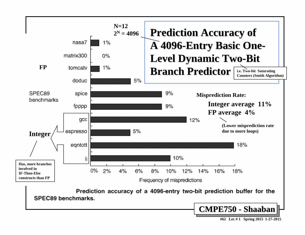
Prediction Accuracy of Prediction Accuracy of A 4096A 4096--Entry Basic OneEntry Basic One--Level Dynamic TwoLevel Dynamic Two--Bit Bit Branch PredictorBranch Predictor
Integer average 11%FP average 4%
Integer
Misprediction Rate:
(Lower misprediction rate due to more loops)
FP
N=122N = 4096
Has, more branchesinvolved in IF-Then-Elseconstructs than FP
i.e. Two-bit SaturatingCounters (Smith Algorithm)

CMPE750 CMPE750 -- ShaabanShaaban#63 Lec # 1 Spring 2015 1-27-2015
Correlating BranchesCorrelating BranchesRecent branches are possibly correlated: The behavior of recently executed branches affects prediction of current branch.
Example:
Branch B3 is correlated with branches B1, B2. If B1, B2 are both not taken, then B3 will be taken. Using only the behavior of one branch cannot detect this behavior.
B1 if (aa==2)aa=0;
B2 if (bb==2)bb=0;
B3 if (aa!==bb){
DSUBUI R3, R1, #2 ; R3 = R1 - 2BNEZ R3, L1 ; B1 (aa!=2)DADD R1, R0, R0 ; aa==0
L1: DSUBUI R3, R2, #2 ; R3 = R2 - 2BNEZ R3, L2 ; B2 (bb!=2)DADD R2, R0, R0 ; bb==0
L2: DSUBUI R3, R1, R2 ; R3=aa-bbBEQZ R3, L3 ; B3 (aa==bb)
(not taken)
(not taken)
Occur in branches used to implement if-then-else constructsWhich are more common in integer than floating point code
Here aa = R1 bb = R2
B1 not taken
B2 not taken
B3 taken if aa=bb
aa=bb=2
(not taken)
+
B3 in this case
Both B1 and B2 Not Taken → B3 Taken

CMPE750 CMPE750 -- ShaabanShaaban#64 Lec # 1 Spring 2015 1-27-2015
Correlating TwoCorrelating Two--Level Dynamic Level Dynamic GApGAp Branch PredictorsBranch Predictors• Improve branch prediction by looking not only at the history of the branch in
question but also at that of other branches using two levels of branch history.• Uses two levels of branch history:
– First level (global): • Record the global pattern or history of the m most recently executed
branches as taken or not taken. Usually an m-bit shift register.– Second level (per branch address):
• 2m prediction tables (PHTs), each table entry has n bit saturating counter.
• The branch history pattern from first level is used to select the proper branch prediction table in the second level.
• The low N bits of the branch address are used to select the correct prediction entry (predictor)within a the selected table, thus each of the 2m tables has 2N entries and each entry is 2 bits counter.
• Total number of bits needed for second level = 2m x n x 2N bits• In general, the notation: GAp (m,n) predictor means:
– Record last m branches to select between 2m history tables.– Each second level table uses n-bit counters (each table entry has n bits).
• Basic two-bit single-level Bimodal BHT is then a (0,2) predictor.
m-bit shift registerLastBranch0 =Not taken1 = Taken
Branch History Register (BHR)
Pattern History Tables (PHTs)
1
2
4th Edition: In Chapter 2.3 (3rd Edition: In Chapter 3.4)

CMPE750 CMPE750 -- ShaabanShaaban#65 Lec # 1 Spring 2015 1-27-2015
Organization of A Correlating Two-level GAp (2,2) Branch Predictor
First LevelBranch HistoryRegister (BHR)(2 bit shift register)
Second Level
m = # of branches tracked in first level = 2Thus 2m = 22 = 4 tables in second level
N = # of low bits of branch address used = 4Thus each table in 2nd level has 2N = 24 = 16 entries
n = # number of bits of 2nd level table entry = 2
Number of bits for 2nd level = 2m x n x 2N
= 4 x 2 x 16 = 128 bits
High bit determines branch prediction0 = Not Taken1 = Taken
Low 4 bits of address
Selects correct table
Selects correct Entry(predictor)in table
GAp
Global(1st level) Adaptive
per address(2nd level)
Branch HistoryRegister (BHR)
(N= 4)
(m = 2)
(n = 2)
Pattern History Tables (PHTs)

CMPE750 CMPE750 -- ShaabanShaaban#66 Lec # 1 Spring 2015 1-27-2015
Prediction Accuracy Prediction Accuracy of Twoof Two--Bit Dynamic Bit Dynamic Predictors Under Predictors Under SPEC89SPEC89
BasicBasic BasicBasic Correlating Correlating TwoTwo--levellevelSingle (one) Level
FP
Integer
N = 12 N = 10
Gap (2, 2)m= 2 n= 2

CMPE750 CMPE750 -- ShaabanShaaban#67 Lec # 1 Spring 2015 1-27-2015
Multiple Instruction Issue: CPI < 1Multiple Instruction Issue: CPI < 1• To improve a pipeline’s CPI to be better [less] than one, and to better exploit
Instruction Level Parallelism (ILP), a number of instructions have to be issued in the same cycle.
• Multiple instruction issue processors are of two types:– Superscalar: A number of instructions (2-8) is issued in the same
cycle, scheduled statically by the compiler or -more commonly-dynamically (Tomasulo).
• PowerPC, Sun UltraSparc, Alpha, HP 8000, Intel PII, III, 4 ...– VLIW (Very Long Instruction Word):
A fixed number of instructions (3-6) are formatted as one long instruction word or packet (statically scheduled by the compiler).
– Example: Explicitly Parallel Instruction Computer (EPIC)• Originally a joint HP/Intel effort.• ISA: Intel Architecture-64 (IA-64) 64-bit address:• First CPU: Itanium, Q1 2001. Itanium 2 (2003)
• Limitations of the approaches:– Available ILP in the program (both).– Specific hardware implementation difficulties (superscalar).– VLIW optimal compiler design issues.
CPI < 1 or CPI < 1 or Instructions Per Cycle (IPC) > 1
Most common = 4 instructions/cyclecalled 4-way superscalar processor
4th Edition: Chapter 2.7(3rd Edition: Chapter 3.6, 4.3
1
2
SpecialISA Needed

CMPE750 CMPE750 -- ShaabanShaaban#68 Lec # 1 Spring 2015 1-27-2015
• Two instructions can be issued per cycle (static two-issue or 2-way superscalar).• One of the instructions is integer (including load/store, branch). The other instruction
is a floating-point operation.– This restriction reduces the complexity of hazard checking.
• Hardware must fetch and decode two instructions per cycle.• Then it determines whether zero (a stall), one or two instructions can be issued (in
decode stage) per cycle.
Simple Statically Scheduled Superscalar PipelineSimple Statically Scheduled Superscalar Pipeline
MEMEXEXEXIDIDIFIF
EXEXIDIDIFIF
WBWBEXMEMEXEXEX
WBWBEXMEMEX
WBWBEX
IDIDIFIF
WBEXMEMEXEXEXIDID
IFIF
Integer Instruction
Integer Instruction
Integer Instruction
Integer Instruction
FP Instruction
FP Instruction
FP Instruction
FP Instruction
1 2 3 4 5 6 7 8Instruction Type
TwoTwo--issue statically scheduled pipeline in operationissue statically scheduled pipeline in operationFP instructions assumed to be adds (EX takes 3 cycles)FP instructions assumed to be adds (EX takes 3 cycles)
Ideal CPI = 0.5 Ideal Instructions Per Cycle (IPC) = 2
Instructions assumed independent (no stalls)
Current Statically Scheduled Superscalar Example: Intel Atom Processor

CMPE750 CMPE750 -- ShaabanShaaban#69 Lec # 1 Spring 2015 1-27-2015
Intel IAIntel IA--64: VLIW “Explicitly Parallel 64: VLIW “Explicitly Parallel Instruction Computing (EPIC)”Instruction Computing (EPIC)”
• Three 41-bit instructions in 128 bit “Groups” or bundles; an instruction bundle template field (5-bits) determines if instructions are dependent or independent and statically specifies the functional units to used by the instructions:– Smaller code size than old VLIW, larger than x86/RISC– Groups can be linked to show dependencies of more than three
instructions.• 128 integer registers + 128 floating point registers• Hardware checks dependencies
(interlocks ⇒ binary compatibility over time)
• Predicated execution: An implementation of conditional instructions used to reduce the number of conditional branches used in the generated code ⇒ larger basic block size
• IA-64 : Name given to instruction set architecture (ISA).• Itanium : Name of the first implementation (2001).
In VLIW dependency analysis is done statically by the compilernot dynamically in hardware (Tomasulo)
Statically scheduledNo register renaming in hardware
i.e statically scheduledby compiler

CMPE750 CMPE750 -- ShaabanShaaban#70 Lec # 1 Spring 2015 1-27-2015
Intel/HP EPIC VLIW ApproachIntel/HP EPIC VLIW Approachoriginal sourceoriginal source
codecode
ExposeExposeInstructionInstructionParallelismParallelism(dependency(dependency
analysis)analysis)OptimizeOptimize
Exploit Exploit InstructionInstructionParallelism:Parallelism:
GenerateGenerateVLIWsVLIWs
compilercompiler
Instruction DependencyInstruction DependencyAnalysisAnalysis
Instruction 2Instruction 2 Instruction 1Instruction 1 Instruction 0Instruction 0 TemplateTemplate
128128--bit bundlebit bundle
00127127
41 bits 41 bits 5 bits41 bits
SequentialCode
Dependency Graph
Template field has static assignment/scheduling information
1
2
3InstructionBundles
IssueSlot

CMPE750 CMPE750 -- ShaabanShaaban#71 Lec # 1 Spring 2015 1-27-2015
Unrolled Loop Example for Unrolled Loop Example for Scalar (singleScalar (single--issue) Pipelineissue) Pipeline
1 Loop: L.D F0,0(R1)2 L.D F6,-8(R1)3 L.D F10,-16(R1)4 L.D F14,-24(R1)5 ADD.D F4,F0,F26 ADD.D F8,F6,F27 ADD.D F12,F10,F28 ADD.D F16,F14,F29 S.D F4,0(R1)10 S.D F8,-8(R1)11 DADDUI R1,R1,#-3212 S.D F12,16(R1)13 BNE R1,R2,LOOP14 S.D F16,8(R1) ; 8-32 = -24
14 clock cycles, or 3.5 per original iteration (result)(unrolled four times)
Latency:L.D to ADD.D: 1 CycleADD.D to S.D: 2 Cycles
Unrolled and scheduled loopfrom loop unrolling example
No stalls in code above: CPI = 1 (ignoring initial pipeline fill cycles)
Recall that loop unrolling exposes more ILPby increasing size of resulting basic block
3.5 = 14/4 cycles

CMPE750 CMPE750 -- ShaabanShaaban#72 Lec # 1 Spring 2015 1-27-2015
Loop Unrolling in 2Loop Unrolling in 2--way Superscalar Pipeline: way Superscalar Pipeline: (1 Integer, 1 FP/Cycle)(1 Integer, 1 FP/Cycle)
Integer instruction FP instruction Clock cycleLoop: L.D F0,0(R1) 1
L.D F6,-8(R1) 2L.D F10,-16(R1) ADD.D F4,F0,F2 3L.D F14,-24(R1) ADD.D F8,F6,F2 4L.D F18,-32(R1) ADD.D F12,F10,F2 5S.D F4,0(R1) ADD.D F16,F14,F2 6S.D F8,-8(R1) ADD.D F20,F18,F2 7S.D F12,-16(R1) 8DADDUI R1,R1,#-40 9S.D F16,-24(R1) 10BNE R1,R2,LOOP 11SD -32(R1),F20 12
• Unrolled 5 times to avoid delays and expose more ILP (unrolled one more time)• 12 cycles, or 12/5 = 2.4 cycles per iteration (3.5/2.4= 1.5X faster than scalar)• CPI = 12/ 17 = .7 worse than ideal CPI = .5 because 7 issue slots are wasted
Empty or wastedissue slot
Recall that loop unrolling exposes more ILP by increasing basic block size
Ideal CPI = 0.5 IPC = 2
Scalar Processor = Single-issue Processor
Unrolled 5 times
12/5 = 2.4 cyclesper original iteration

CMPE750 CMPE750 -- ShaabanShaaban#73 Lec # 1 Spring 2015 1-27-2015
Loop Unrolling in VLIW PipelineLoop Unrolling in VLIW Pipeline(2 Memory, 2 FP, 1 Integer / Cycle)(2 Memory, 2 FP, 1 Integer / Cycle)
Memory Memory FP FP Int. op/ Clockreference 1 reference 2 operation 1 op. 2 branchL.D F0,0(R1) L.D F6,-8(R1) 1L.D F10,-16(R1) L.D F14,-24(R1) 2L.D F18,-32(R1) L.D F22,-40(R1) ADD.D F4,F0,F2 ADD.D F8,F6,F2 3L.D F26,-48(R1) ADD.D F12,F10,F2 ADD.D F16,F14,F2 4
ADD.D F20,F18,F2 ADD.D F24,F22,F2 5S.D F4,0(R1) S.D F8, -8(R1) ADD.D F28,F26,F2 6S.D F12, -16(R1) S.D F16,-24(R1) DADDUI R1,R1,#-56 7S.D F20, 24(R1) S.D F24,16(R1) 8S.D F28, 8(R1) BNE R1,R2,LOOP 9
Unrolled 7 times to avoid delays and expose more ILP7 results in 9 cycles, or 1.3 cycles per iteration
(2.4/1.3 =1.8X faster than 2-issue superscalar, 3.5/1.3 = 2.7X faster than scalar)Average: about 23/9 = 2.55 IPC (instructions per clock cycle) Ideal IPC =5, CPI = .39 Ideal CPI = .2 thus about 50% efficiency, 22 issue slots are wasted
Note: Needs more registers in VLIW (15 vs. 6 in Superscalar)
Empty or wastedissue slot
5-issue VLIWIdeal CPI = 0.2
IPC = 5
Scalar Processor = Single-Issue Processor4th Edition: Chapter 2.7 pages 116-117(3rd Edition: Chapter 4.3 pages 317-318)
9/7 = 1.3 cyclesper original iteration
Total =22

CMPE750 CMPE750 -- ShaabanShaaban#74 Lec # 1 Spring 2015 1-27-2015
• Empty or wasted issue slots can be defined as either vertical waste or horizontal waste:
– Vertical waste is introduced when the processor issues no instructions in a cycle.
– Horizontal waste occurs when not all issue slots can be filled in a cycle.
Superscalar Architecture Limitations:Superscalar Architecture Limitations:Issue Slot Waste Classification
Example:
4-IssueSuperscalar
Ideal IPC =4Ideal CPI = .25
Instructions Per Cycle = IPC = 1/CPIAlso applies to VLIW
Result of issue slot waste: Actual Performance << Peak Performance
Time

CMPE750 CMPE750 -- ShaabanShaaban#75 Lec # 1 Spring 2015 1-27-2015
Speculation (Speculative Execution) Speculation (Speculative Execution) • Compiler ILP techniques (loop-unrolling, software Pipelining etc.) are not effective to
uncover maximum ILP when branch behavior is not well known at compile time. • Full exploitation of the benefits of dynamic branch prediction and further reduction of the
impact of branches on performance can be achieved by using speculation:
– Speculation: An instruction is executed before the processor knows that the instruction should execute to avoid control dependence stalls (i.e. branch not resolved yet):
• Static Speculation by the compiler with hardware support:– The compiler labels an instruction as speculative and the hardware
helps by ignoring the outcome of incorrectly speculated instructions.– Conditional instructions provide limited speculation.
• Dynamic Hardware-based Speculation: – Uses dynamic branch-prediction to guide the speculation process.– Dynamic scheduling and execution continued passed a conditional
branch in the predicted branch direction.
No ISAor CompilerSupport Needed
ISA/CompilerSupport Needed
e.g dynamic speculative execution
Further Reduction of Impact of Branches on Performance of Pipelined Processors:
Here we focus on hardware-based speculation using Tomasulo-based dynamic scheduling enhanced with speculation (Speculative Tomasulo).
• The resulting processors are usually referred to as Speculative Processors.
4th Edition: Chapter 2.6, 2.8(3rd Edition: Chapter 3.7)

CMPE750 CMPE750 -- ShaabanShaaban#76 Lec # 1 Spring 2015 1-27-2015
Dynamic HardwareDynamic Hardware--Based SpeculationBased Speculation•• Combines:Combines:
– Dynamic hardware-based branch prediction– Dynamic Scheduling: issue multiple instructions in order and
execute out of order. (Tomasulo)• Continue to dynamically issue, and execute instructions passed
a conditional branch in the dynamically predicted branch direction, before control dependencies are resolved.– This overcomes the ILP limitations of the basic block size.– Creates dynamically speculated instructions at run-time with no
ISA/compiler support at all.– If a branch turns out as mispredicted all such dynamically
speculated instructions must be prevented from changing the state of the machine (registers, memory).
• Addition of commit (retire, completion, or re-ordering) stage and forcing instructions to commit in their order in the code (i.e to write results to registers or memory in program order).
• Precise exceptions are possible since instructions must commit in order.
How?
(Speculative Execution Processors, Speculative Tomasulo)
i.e speculated instructions must be cancelled
Why?i.e. before branch
is resolved
i.e Dynamic speculative execution
i.e instructions forced to complete (commit) in program order
4th Edition: Chapter 2.6, 2.8 (3rd Edition: Chapter 3.7)
1
2
Branchmispredicted?

CMPE750 CMPE750 -- ShaabanShaaban#77 Lec # 1 Spring 2015 1-27-2015
HardwareHardware--Based Based SpeculationSpeculation
Usuallyimplemented as a circularbuffer
StoreResults
Commit or RetirementFIFO
4th Edition: page 107 (3rd Edition: page 228)
Speculative Tomasulo-based Processor
(In Order)
Speculative Execution +Speculative Execution +Tomasulo’s AlgorithmTomasulo’s Algorithm
= Speculative Tomasulo
Instructionsto issue in Order:InstructionQueue (IQ)
Next tocommit

CMPE750 CMPE750 -- ShaabanShaaban#78 Lec # 1 Spring 2015 1-27-2015
Four Steps of Speculative Tomasulo AlgorithmFour Steps of Speculative Tomasulo Algorithm1. Issue — (In-order) Get an instruction from Instruction Queue
If a reservation station and a reorder buffer slot are free, issue instruction & send operands & reorder buffer number for destination (this stage is sometimes called “dispatch”)
2. Execution — (out-of-order) Operate on operands (EX)When both operands are ready then execute; if not ready, watch CDB for result; when both operands are in reservation station, execute; checks RAW (sometimes called “issue”)
3. Write result — (out-of-order) Finish execution (WB)Write on Common Data Bus (CDB) to all awaiting FUs & reorder buffer; mark reservation station available.
4. Commit — (In-order) Update registers, memory with reorder buffer result– When an instruction is at head of reorder buffer & the result is present,
update register with result (or store to memory) and remove instruction from reorder buffer.
– A mispredicted branch at the head of the reorder buffer flushes the reorder buffer (cancels speculated instructions after the branch)
⇒ Instructions issue in order, execute (EX), write result (WB) out of order, but must commit in order.
Stage 0 Instruction Fetch (IF): No changes, in-order
i.e Reservation Stations
No write to registers or memory in WB
Includes data MEM read
4th Edition: pages 106-108 (3rd Edition: pages 227-229)
No WB for storesor branches
Successfully completed instructions write to registers and memory (stores) hereMispredictedBranchHandling

CMPE750 CMPE750 -- ShaabanShaaban#79 Lec # 1 Spring 2015 1-27-2015
Memory Hierarchy: MotivationMemory Hierarchy: MotivationProcessorProcessor--Memory (DRAM) Performance GapMemory (DRAM) Performance Gap
µProc60%/yr.
DRAM7%/yr.
1
10
100
100019
8019
81
1983
1984
1985
1986
1987
1988
1989
1990
1991
1992
1993
1994
1995
1996
1997
1998
1999
2000
DRAM
CPU19
82
Processor-MemoryPerformance Gap:(grows 50% / year)
Perf
orm
ance
i.e. Gap between memory access time (latency) and CPU cycle timeMemory Access Latency: The time between a memory access request is issued by the processor and the time the requested information (instructions or data) is available to the processor.
Ideal Memory Access Time (latency) = 1 CPU CycleReal Memory Access Time (latency) >> 1 CPU cycle

CMPE750 CMPE750 -- ShaabanShaaban#80 Lec # 1 Spring 2015 1-27-2015
Memory Access LatencyReduction & Hiding Techniques
Memory Latency Reduction Techniques:• Faster Dynamic RAM (DRAM) Cells: Depends on VLSI processing technology.• Wider Memory Bus Width: Fewer memory bus accesses needed (e.g 128 vs. 64 bits)• Multiple Memory Banks:
– At DRAM chip level (SDR, DDR SDRAM), module or channel levels.• Integration of Memory Controller with Processor: e.g AMD’s current processor architecture• New Emerging Faster RAM Technologies: e.g. Magnetoresistive Random Access Memory (MRAM)
Memory Latency Hiding Techniques:
–– Memory HierarchyMemory Hierarchy: One or more levels of smaller and faster memory (SRAM-based cache) on- or off-chip that exploit program access locality to hide long main memory latency.
– Pre-Fetching: Request instructions and/or data from memory before actually needed to hide long memory access latency.
Addressing The CPU/Memory Performance Gap:
What about dynamic scheduling?
Reduce it!
Hide it!
Get it from main memory into cache before you need it !

CMPE750 CMPE750 -- ShaabanShaaban#81 Lec # 1 Spring 2015 1-27-2015
Memory Hierarchy: MotivationMemory Hierarchy: Motivation• The gap between CPU performance and main memory has been widening
with higher performance CPUs creating performance bottlenecks for memory access instructions.
• To hide long memory access latency, the memory hierarchy is organized into several levels of memory with the smaller, faster SRAM-based memory levels closer to the CPU: registers, then primary Cache Level (L1), then additional secondary cache levels (L2, L3…), then DRAM-based main memory, then mass storage (virtual memory).
• Each level of the hierarchy is usually a subset of the level below: data found in a level is also found in the level below (farther from CPU) but at lower speed (longer access time).
• Each level maps addresses from a larger physical memory to a smaller level of physical memory closer to the CPU.
• This concept is greatly aided by the principal of locality both temporal and spatial which indicates that programs tend to reuse data and instructions that they have used recently or those stored in their vicinity leading to working set of a program.
For Ideal Memory: Memory Access Time or latency = 1 CPU cycle
Addressing CPU/Memory Performance Gap by Hiding Long Memory Latency:
Both Editions: Chapter 5.1

CMPE750 CMPE750 -- ShaabanShaaban#82 Lec # 1 Spring 2015 1-27-2015
Basic Cache Design & Operation IssuesBasic Cache Design & Operation Issues• Q1: Where can a block be placed cache?
(Block placement strategy & Cache organization)– Fully Associative, Set Associative, Direct Mapped.
• Q2: How is a block found if it is in cache? (Block identification)– Tag/Block.
• Q3: Which block should be replaced on a miss? (Block replacement)– Random, LRU, FIFO.
• Q4: What happens on a write? (Cache write policy)– Write through, write back.
Cache Hit/Miss?
Tag Matching
Locating a block
Block placement
4th Edition: Appendix C.1 (3rd Edition Chapter 5.2)
Block replacement
+ Cache block write allocation policy

CMPE750 CMPE750 -- ShaabanShaaban#83 Lec # 1 Spring 2015 1-27-2015
Cache Organization & Placement StrategiesCache Organization & Placement StrategiesPlacement strategies or mapping of a main memory data block ontocache block frames divide cache designs into three organizations:1 Direct mapped cache: A block can be placed in only one location
(cache block frame), given by the mapping function:index = (Block address) MOD (Number of blocks in cache)
2 Fully associative cache: A block can be placed anywhere in cache. (no mapping function).
3 Set associative cache: A block can be placed in a restricted set of places, or cache block frames. A set is a group of block frames in the cache. A block is first mapped onto the set and then it can be placed anywhere within the set. The set in this case is chosen by:
index = (Block address) MOD (Number of sets in cache)
If there are n blocks in a set the cache placement is called n-way set-associative.
Mapping Function
Mapping Function
Most common cache organization
Most complex cache organization to implement
Least complex to implementsuffers from conflict misses

CMPE750 CMPE750 -- ShaabanShaaban#84 Lec # 1 Spring 2015 1-27-2015
Address Field Sizes/MappingAddress Field Sizes/Mapping
Block Address BlockOffsetTag Index
Block offset size = log2(block size)
Index size = log2(Total number of blocks/associativity)
Tag size = address size Tag size = address size -- index size index size -- offset sizeoffset size
Physical Memory Address Generated by CPU
Mapping function:Cache set or block frame number = Index =
= (Block Address) MOD (Number of Sets)
Number of Setsin cache
No index/mapping function for fully associative cache
(size determined by amount of physical main memory cacheable)

CMPE750 CMPE750 -- ShaabanShaaban#85 Lec # 1 Spring 2015 1-27-2015
Index Field(8 bits)
TagField (22 bits)
Block Offset Field(2 bits)
4K Four4K Four--Way Set Associative Cache:Way Set Associative Cache:MIPS Implementation ExampleMIPS Implementation Example
Ad dress
2 2 8
V TagIndex
012
253254255
D ata V Tag D ata V T ag D ata V T ag D ata
3222
4 - to - 1 m ultip lexo r
H it D a ta
123891011123 031 0
1024 block framesEach block = one word4-way set associative1024 / 4= 28= 256 sets
Can cache up to232 bytes = 4 GBof memory
Block Address = 30 bits
Tag = 22 bits Index = 8 bitsBlock offset = 2 bits
Set associative cache requires parallel tag matching and more complex hit logic which may increase hit time
Tag Index Offset
SRAM
Hit/MissLogic
Mapping Function: Cache Set Number = index= (Block address) MOD (256)
Hit Access Time = SRAM Delay + Hit/Miss Logic Delay
Set Number
Mapping
Typically, primary or Level 1 (L1) cache is 2-8 way set associative

CMPE750 CMPE750 -- ShaabanShaaban#86 Lec # 1 Spring 2015 1-27-2015
Memory HierarchyHierarchy Performance:Average Memory Access Time (AMAT), Memory Stall cycles
• The Average Memory Access Time (AMAT): The number of cycles required to complete an average memory access request by the CPU.
• Memory stall cycles per memory access: The number of stall cycles added to CPU execution cycles for one memory access.
• Memory stall cycles per average memory access = (AMAT -1)• For ideal memory: AMAT = 1 cycle, this results in zero memory stall
cycles.• Memory stall cycles per average instruction =
Number of memory accesses per instructionx Memory stall cycles per average memory access
= ( 1 + fraction of loads/stores) x (AMAT -1 )
Base CPI = CPIexecution = CPI with ideal memory
CPI = CPIexecution + Mem Stall cycles per instruction
Instruction Fetch
cycles = CPU cycles
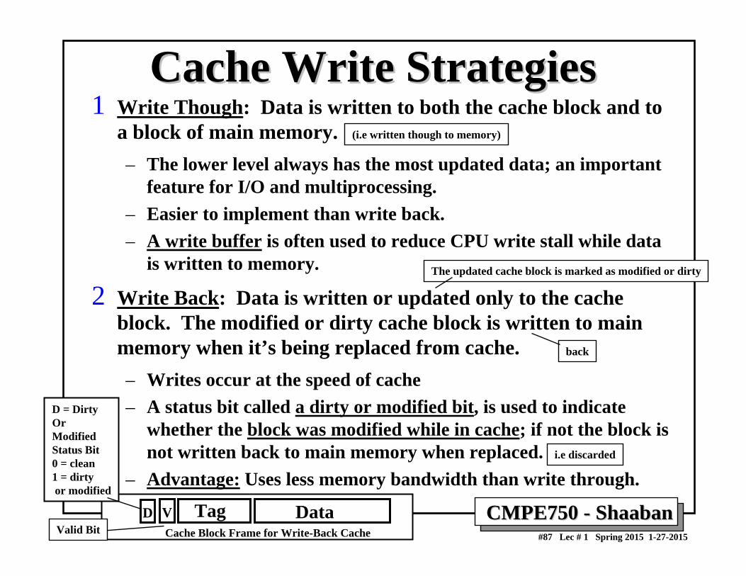
CMPE750 CMPE750 -- ShaabanShaaban#87 Lec # 1 Spring 2015 1-27-2015
Cache Write StrategiesCache Write Strategies1 Write Though: Data is written to both the cache block and to
a block of main memory.– The lower level always has the most updated data; an important
feature for I/O and multiprocessing.– Easier to implement than write back.– A write buffer is often used to reduce CPU write stall while data
is written to memory.
2 Write Back: Data is written or updated only to the cache block. The modified or dirty cache block is written to main memory when it’s being replaced from cache.– Writes occur at the speed of cache– A status bit called a dirty or modified bit, is used to indicate
whether the block was modified while in cache; if not the block is not written back to main memory when replaced.
– Advantage: Uses less memory bandwidth than write through.
(i.e written though to memory)
back
The updated cache block is marked as modified or dirty
DataTagVD
D = DirtyOr ModifiedStatus Bit0 = clean1 = dirtyor modified
Cache Block Frame for Write-Back CacheValid Bit
i.e discarded

CMPE750 CMPE750 -- ShaabanShaaban#88 Lec # 1 Spring 2015 1-27-2015
Cache Write Miss PolicyCache Write Miss Policy• Since data is usually not needed immediately on a write miss two
options exist on a cache write miss:Write Allocate:The missed cache block is loaded into cache on a write miss followed by write hit actions.
No-Write Allocate:The block is modified in the lower level (lower cache level, or main memory) and not loaded (written or updated) into cache.
While any of the above two write miss policies can be used with either write back or write through:
• Write back caches always use write allocate to capturesubsequent writes to the block in cache.
• Write through caches usually use no-write allocate since subsequent writes still have to go to memory.
Cache Write Miss = Block to be modified is not in cacheAllocate = Allocate or assign a cache block frame for written data
i.e A cache block frame is allocated for the block to be modified (written-to)
i.e A cache block frame is not allocated for the block to be modified (written-to)
(Bring old block to cache then update it)

CMPE750 CMPE750 -- ShaabanShaaban#89 Lec # 1 Spring 2015 1-27-2015
Memory Access Tree, Unified L1Write Through, No Write Allocate, No Write Buffer
CPU Memory Access
Read Write
L1 Write Miss:Access Time : M + 1
Stalls per access = M Stalls = % write x (1 - H1 ) x M
L1 Write Hit:Access Time: M +1Stalls Per access = M
Stalls =% write x (H1 ) x M
L1 Read Hit:Hit Access Time = 1Stalls = 0
L1 Read Miss:Access Time = M + 1Stalls Per access = MStalls = % reads x (1 - H1 ) x M
Stall Cycles Per Memory Access = % reads x (1 - H1 ) x M + % write x M
AMAT = 1 + % reads x (1 - H1 ) x M + % write x M
CPI = CPIexecution + (1 + fraction of loads/stores) x Stall Cycles per access
Stall Cycles per access = AMAT - 1
M = Miss PenaltyH1 = Level 1 Hit Rate1- H1 = Level 1 Miss Rate
% write% reads
% reads x (1 - H1 )% reads x H1 % write x (1 - H1 )% write x H1
100%or 1
M = Miss Penalty = stall cycles per access resulting from missing in cacheM + 1 = Miss Time = Main memory access timeH1 = Level 1 Hit Rate 1- H1 = Level 1 Miss Rate
Assuming:Ideal access on a read hit, no stalls
Exercise:Create memory access tree for split level 1
Unified
L1
Instruction Fetch + Loads
Stores

CMPE750 CMPE750 -- ShaabanShaaban#90 Lec # 1 Spring 2015 1-27-2015
Memory Access Tree Unified L1Write Back, With Write Allocate
CPU Memory Access
L1 MissL1 Hit:
% = H1Hit Access Time = 1Stalls = 0
Stall Cycles Per Memory Access = (1-H1) x ( M x % clean + 2M x % dirty )
AMAT = 1 + Stall Cycles Per Memory Access
CPI = CPIexecution + (1 + fraction of loads/stores) x Stall Cycles per access
L1 Miss, CleanAccess Time = M +1Stalls per access = M Stall cycles = M x (1 -H1) x % clean
L1 Miss, DirtyAccess Time = 2M +1Stalls per access = 2M Stall cycles = 2M x (1-H1) x % dirty
H1(1-H1)
(1-H1) x % dirty(1 -H1) x % clean
1 or 100%
M = Miss Penalty = stall cycles per access resulting from missing in cacheM + 1 = Miss Time = Main memory access timeH1 = Level 1 Hit Rate 1- H1 = Level 1 Miss Rate
Assuming:Ideal access on a hit, no stalls
Unified
L1
2M needed to:- Write (back) Dirty Block- Read new block
(2 main memory accesses needed)
One access to main memory to get needed block
2M = M + M
Write backdirty block
Get neededblock in cache(allocate frame)
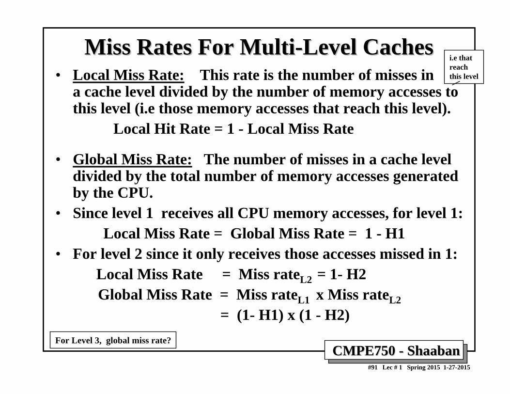
CMPE750 CMPE750 -- ShaabanShaaban#91 Lec # 1 Spring 2015 1-27-2015
Miss Rates For MultiMiss Rates For Multi--Level CachesLevel Caches• Local Miss Rate: This rate is the number of misses in
a cache level divided by the number of memory accesses to this level (i.e those memory accesses that reach this level).
Local Hit Rate = 1 - Local Miss Rate
• Global Miss Rate: The number of misses in a cache level divided by the total number of memory accesses generated by the CPU.
• Since level 1 receives all CPU memory accesses, for level 1:Local Miss Rate = Global Miss Rate = 1 - H1
• For level 2 since it only receives those accesses missed in 1: Local Miss Rate = Miss rateL2 = 1- H2Global Miss Rate = Miss rateL1 x Miss rateL2
= (1- H1) x (1 - H2)For Level 3, global miss rate?
i.e thatreachthis level

CMPE750 CMPE750 -- ShaabanShaaban#92 Lec # 1 Spring 2015 1-27-2015
Common Write Policy For 2-Level Cache• Write Policy For Level 1 Cache:
– Usually Write through to Level 2.– Write allocate is used to reduce level 1 read misses.– Use write buffer to reduce write stalls to level 2.
• Write Policy For Level 2 Cache:– Usually write back with write allocate is used.
• To minimize memory bandwidth usage.
• The above 2-level cache write policy results in inclusive L2 cachesince the content of L1 is also in L2
• Common in the majority of all CPUs with 2-levels of cache• As opposed to exclusive L1, L2 (e.g AMD Athlon XP, A64)
i.e what is in L1 is not duplicated in L2
L1 L2
As if we have a single level of cache with one portion (L1) is faster than remainder (L2)
L1
L2
(not write through to main memory just to L2)

CMPE750 CMPE750 -- ShaabanShaaban#93 Lec # 1 Spring 2015 1-27-2015
22--Level (Both Unified) Memory Access TreeLevel (Both Unified) Memory Access TreeL1: Write Through to L2, Write Allocate, With Perfect Write BuffL1: Write Through to L2, Write Allocate, With Perfect Write Bufferer
L2: Write Back with Write AllocateL2: Write Back with Write Allocate
CPU Memory Access
L1 Miss:L1 Hit:Hit Access Time = 1Stalls Per access = 0
L1 Miss, L2 Hit:Hit Access Time =T2 +1Stalls per L2 Hit = T2Stalls = (1-H1) x H2 x T2
(1-H1)(H1)
L1 Miss, L2 Miss
(1-H1) x (1-H2)
L1 Miss, L2 Miss, CleanAccess Time = M +1Stalls per access = M Stall cycles = M x (1 -H1) x (1-H2) x % clean
L1 Miss, L2 Miss, DirtyAccess Time = 2M +1Stalls per access = 2M Stall cycles = 2M x (1-H1) x (1-H2) x % dirty
Stall cycles per memory access = (1-H1) x H2 x T2 + M x (1 -H1) x (1-H2) x % clean + 2M x (1-H1) x (1-H2) x % dirty
= (1-H1) x H2 x T2 + (1 -H1) x (1-H2) x ( % clean x M + % dirty x 2M)
AMAT = 1 + Stall Cycles Per Memory AccessCPI = CPIexecution + (1 + fraction of loads and stores) x Stall Cycles per access
(1-H1) x H2
1 or 100%
(1-H1) x (1-H2) x % dirty(1 -H1) x (1-H2) x % clean
Assuming:Ideal access on a hit in L1T1 = 0
Global Miss Rate for L2
Unified
L2
Unified
L1

CMPE750 CMPE750 -- ShaabanShaaban#94 Lec # 1 Spring 2015 1-27-2015
Cache Optimization SummaryCache Optimization SummaryTechnique MR MP HT ComplexityLarger Block Size + – 0Higher Associativity + – 1Victim Caches + 2Pseudo-Associative Caches + 2HW Prefetching of Instr/Data + 2Compiler Controlled Prefetching + 3Compiler Reduce Misses + 0Priority to Read Misses + 1Subblock Placement + + 1Early Restart & Critical Word 1st + 2Non-Blocking Caches + 3Second Level Caches + 2Small & Simple Caches – + 0Avoiding Address Translation + 2Pipelining Writes + 1
Mis
s ra
teH
it tim
eM
iss
Pena
lty

CMPE750 CMPE750 -- ShaabanShaaban#95 Lec # 1 Spring 2015 1-27-2015
X86 CPU Cache/Memory Performance Example:X86 CPU Cache/Memory Performance Example:AMD AMD AthlonAthlon XP/64/FX Vs. Intel P4/Extreme EditionXP/64/FX Vs. Intel P4/Extreme Edition
Main Memory: Dual (64-bit) Channel PC3200 DDR SDRAMpeak bandwidth of 6400 MB/s
Intel P4 3.2 GHzExtreme EditionData L1: 8KBData L2: 512 KBData L3: 2048 KB
Intel P4 3.2 GHzData L1: 8KBData L2: 512 KB
AMD Athon XP 2.2 GHzData L1: 64KBData L2: 512 KB (exclusive)
Source: The Tech Report 1-21-2004http://www.tech-report.com/reviews/2004q1/athlon64-3000/index.x?pg=3
AMD Athon 64 FX51 2.2 GHzData L1: 64KBData L2: 1024 KB (exlusive)
AMD Athon 64 3400+ 2.2 GHzData L1: 64KBData L2: 1024 KB (exclusive)
AMD Athon 64 3000+ 2.0 GHzData L1: 64KBData L2: 512 KB (exclusive)
AMD Athon 64 3200+ 2.0 GHzData L1: 64KBData L2: 1024 KB (exclusive)

CMPE750 CMPE750 -- ShaabanShaaban#96 Lec # 1 Spring 2015 1-27-2015
• Virtual memory controls two levels of the memory hierarchy: • Main memory (DRAM). • Mass storage (usually magnetic disks).
• Main memory is divided into blocks allocated to different running processes in the system by the OS:
• Fixed size blocks: Pages (size 4k to 64k bytes). (Most common)• Variable size blocks: Segments (largest size 216 up to 232).• Paged segmentation: Large variable/fixed size segments divided into a number
of fixed size pages (X86, PowerPC).
• At any given time, for any running process, a portion of its data/code is loaded (allocated) in main memory while the rest is available only in mass storage.
• A program code/data block needed for process execution and not present in main memory result in a page fault (address fault) and the page has to be loaded into main memory by the OS from disk (demand paging).
• A program can be run in any location in main memory or disk by using a relocation/mapping mechanism controlled by the operating system which maps (translates) the address from virtual address space (logical program address) to physical address space (main memory, disk).
Virtual Memory: OverviewVirtual Memory: Overview
Superpages can be much larger
Using page tables

CMPE750 CMPE750 -- ShaabanShaaban#97 Lec # 1 Spring 2015 1-27-2015
Basic Virtual Memory Management• Operating system makes decisions regarding which virtual
(logical) pages of a process should be allocated in real physical memory and where (demand paging) assisted with hardware Memory Management Unit (MMU)
• On memory access -- If no valid virtual page to physical page translation (i.e page not allocated in main memory)
– Page fault to operating system– Operating system requests page from disk– Operating system chooses page for replacement
• writes back to disk if modified
– Operating system allocates a page in physical memory and updates page table w/ new page table entry (PTE).
Paging is assumed
(e.g system call to handle page fault))
Then restartfaulting process

CMPE750 CMPE750 -- ShaabanShaaban#98 Lec # 1 Spring 2015 1-27-2015
Virtual Memory Basic StrategiesVirtual Memory Basic Strategies• Main memory page placement(allocation): Fully associative
placement or allocation (by OS) is used to lower the miss rate.• Page replacement: The least recently used (LRU) page is replaced
when a new page is brought into main memory from disk.• Write strategy: Write back is used and only those pages changed in
main memory are written to disk (dirty bit scheme is used).• Page Identification and address translation: To locate pages in main
memory a page table is utilized to translate from virtual page numbers (VPNs) to physical page numbers (PPNs) . The page table is indexed by the virtual page number and contains the physical address of the page.– In paging: Offset is concatenated to this physical page address.– In segmentation: Offset is added to the physical segment address.
• Utilizing address translation locality, a translation look-aside buffer (TLB) is usually used to cache recent address translations (PTEs) and prevent a second memory access to read the page table.
PTE = Page Table Entry

CMPE750 CMPE750 -- ShaabanShaaban#99 Lec # 1 Spring 2015 1-27-2015
Direct Page Table OrganizationDirect Page Table Organization
Page offsetVirtual page number
Virtual address
PageoffsetPhysical pagenumber
Physical address
Physical page numberV a lid
If 0 then page is notpresent in memory
Pagetableregister
Pagetable
2 0 1 2
18
3 1 30 2 9 2 8 2 7 1 5 1 4 1 3 12 1 1 1 0 9 8 3 2 1 0
2 9 2 8 2 7 1 5 1 4 1 3 1 2 1 1 1 0 9 8 3 2 1 0
Two memory accesses needed:• First to page table.• Second to item.
•Page table usually inmain memory.
PTEs
PPN
VPN
Paging is assumed
VPN
(PPN)
How to speedup virtual to physical address translation?

CMPE750 CMPE750 -- ShaabanShaaban#100 Lec # 1 Spring 2015 1-27-2015
Speeding Up Address Translation:Speeding Up Address Translation:Translation Translation LookasideLookaside Buffer (TLB)Buffer (TLB)
•• Translation Translation LookasideLookaside Buffer (TLB)Buffer (TLB) : Utilizing address reference temporal
locality, a small on-chip cache used for address translations (PTEs).– TLB entries usually 32-128– High degree of associativity usually used– Separate instruction TLB (I-TLB) and data TLB (D-TLB) are usually used.– A unified larger second level TLB is often used to improve TLB performance
and reduce the associativity of level 1 TLBs.
• If a virtual address is found in TLB (a TLB hit), the page table in main memory is not accessed.
• TLB-Refill: If a virtual address is not found in TLB, a TLB miss (TLB fault) occurs and the system must search (walk) the page table for the appropriate entry and place it into the TLB this is accomplished by the TLB-refill mechanism .
• Types of TLB-refill mechanisms:
– Hardware-managed TLB: A hardware finite state machine is used to refill the TLB on a TLB miss by walking the page table. (PowerPC, IA-32)
– Software-managed TLB: TLB refill handled by the operating system. (MIPS, Alpha, UltraSPARC, HP PA-RISC, …)
Fast but not flexible
i.e. recently used PTEs

CMPE750 CMPE750 -- ShaabanShaaban#101 Lec # 1 Spring 2015 1-27-2015
Speeding Up Address Translation:Speeding Up Address Translation:
Translation Translation LookasideLookaside Buffer (TLB)Buffer (TLB)
111101101101
111101
Physical Memory
Disk Storage
TLB (on-chip)32-128 Entries
Physical PageAddress
Virtual PageNumber
Page Table(in main memory)
Physical Pageor Disk Address
TagValid
Valid
TLB Hits
TLB Misses/Faults(must refill TLB)
Page Faults
PPN
(VPN)
Page Table Entry (PTE)
PPN
Paging is assumed
• TLB: A small on-chip cache that contains recent address translations (PTEs).• If a virtual address is found in TLB (a TLB hit), the page table in main memory is not
accessed. Single-levelUnified TLB shown
Recommended


![Instruction Set Architecture (ISA)meseec.ce.rit.edu/eecc551-fall2000/551-9-12-2000.pdf · 2000. 9. 12. · Instruction Set Architecture (ISA) “... the attributes of a [computing]](https://img.dokumen.tips/doc/110x75/61026047fa8db44d1f2dce1d/instruction-set-architecture-isa-2000-9-12-instruction-set-architecture-isa.jpg)

