A Survey of Decision Tree Classifier Methodology
S. Rasoul Safavian and David LandgrebeSchool of Electrical Engineering
Purdue University, West Lafayette, IN 47907Phone 317-494-3486; Fax 317-494-3358
Copyright (c) 1991 Institute of Electrical and Electronics Engineers. Reprinted from IEEE
Transactions on Systems, Man, and Cybernetics, IEEE Transactions on Systems, Man, and
Cybernetics, Vol. 21, No. 3, pp 660-674, May 1991.
This material is posted here with permission of the IEEE. Internal or personal use of this material is
permitted. However, permission to reprint/republish this material for advertising or promotional
purposes or for creating new collective works for resale or redistribution must be obtained from the
IEEE by sending a blank email message to [email protected].
By choosing to view this document, you agree to all provisions of the copyright laws protecting it.

Safavian & Landgrebe: Survey of Decision Tree Classifier Methodology
A SURVEY OF DECISION TREE CLASSIFIER METHODOLOGY1
by
S. Rasoul Safavian and David LandgrebeSchool of Electrical Engineering
Purdue University, West Lafayette, IN 47907
Abstract - Decision Tree Classifiers (DTC's) are used successfully in many diverse areas such
as radar signal classification, character recognition, remote sensing, medical diagnosis, expert
systems, and speech recognition, to name only a few. Perhaps, the most important feature of
DTC's is their capability to break down a complex decision-making process into a collection of
simpler decisions, thus providing a solution which is often easier to interpret. This paper presents a
survey of current methods for DTC designs and the various existing issues. After considering
potential advantages of DTC's over single stage classifiers, the subjects of tree structure design,
feature selection at each internal node, and decision and search strategies are discussed. Some
remarks concerning the relation between decision trees and Neural Networks (NN) are also made.
I. INTRODUCTION
The decision tree classifier is one of the possible approaches to multistage decision making; table
look-up rules [34], decision table conversion to optimal decision trees [36],[43],[57],[94], and
sequential approaches [22],[80] are others. The basic idea involved in any multistage approach is
to break up a complex decision into a union of several simpler decisions, hoping the final solution
obtained this way would resemble the intended desired solution. A complete review of multistage
recognition schemes is given by Dattatreya and Kanal [14]. Some of the differences between the
different multistage schemes are addressed in Kulkarni & Kanal [45]. The emphasis of this paper
is on the hierarchical approaches. Hierarchical classifiers are a special type of multistage classifiers
which allow rejection of class labels at intermediate stages.
1 The work reported in this paper was supported in part by NSF Grant ECS 8507405 & NASA Grant NAGW-925
IEEE Trans. Systems, Man, & Cybernetics - 2 - May 1991

Safavian & Landgrebe: Survey of Decision Tree Classifier Methodology
The organization of the paper is as follows: Section II contains the preliminaries, definitions, and
terminologies needed for later sections; section III explains the motivations behind DTC's and their
potential use and drawbacks; section IV addresses the problems of tree structure design, feature
selection and decision rules to be used at each internal node. Tree structure design is considered
from top-down, bottom-up, hybrid, and tree growing-pruning points of view. In considering the
feature subset selection at the internal nodes of the tree, a newly proposed approach based on
application of neural networks is considered. Some possible search strategies are also mentioned in
this section. These problems are addressed from the Bayesian, the decision-theoretic, and the
information theoretic and entropy reduction approaches. Other issues such as incremental tree
design, the tree capability to generalize, the missing data value problem, the robustness of tree
design, and the relation between decision trees and neural networks are discussed in section V.
Final comments and conclusions are provided in section VI.
II. PRELIMINARIES
We briefly describe some necessary terminology for describing trees (see Aho et. al. [3] for more
details).
Definitions:
1) A graph G = (V, E) consists of a finite, non-empty set of nodes (or vertices) V
and a set of edges E. If the edges are ordered pairs (v,w) of vertices, then the
graph is said to be directed.
2) A path in a graph is a sequence of edges of the form (v1, v
2), (v
2, v
3), ...,
(vn-1
, vn). We say the path is from v1 to vn
and is of the length n.
3) A directed graph with no cycles is called a directed acyclic graph. A directed
(or rooted) tree is a directed acyclic graph satisfying the following properties:
IEEE Trans. Systems, Man, & Cybernetics - 3 - May 1991

Safavian & Landgrebe: Survey of Decision Tree Classifier Methodology
i) There is exactly one node, called the root, which no edges enter. The
root node contains all the class labels.
ii) Every node except the root has exactly one entering edge.
iii) There is a unique path from the root to each node.
4) If (v,w) is an edge in a tree, then v is called the father of w , and w is a son of
v. If there is a path from v to w (v ≠w), then v is a proper ancestor of w and w
is a proper descendant of v.
5) A node with no proper descendant is called a leaf (or a terminal). All other
nodes (except the root) are called internal nodes.
6) The depth of a node v in a tree is the length of the path from the root to v. The
height of node v in a tree is the length of a largest path from v to a leaf. The
height of a tree is the height of its root. The level of a node v in a tree is the
height of the tree minus the depth of v.
7) An ordered tree is a tree in which the sons of each node are ordered (normally
from left to right).
8) A binary tree is an ordered tree such that
i) each son of a node is distinguished either as a left son or as a right son, and
ii) no node has more than one left son nor more than one right son.
9) The balance of a node v in a binary tree is (1+ L)/(2 + L + R), where L and R
are the number of nodes in the left and right subtrees of v. A binary tree is
α - balanced , 0 < α <= 1, if every node has balance between α and 1 - α. A 21 - balanced binary tree is also known as a complete tree.
We will denote any tree by T. See Figure 1 for an example of a general decision tree.
IEEE Trans. Systems, Man, & Cybernetics - 4 - May 1991

Safavian & Landgrebe: Survey of Decision Tree Classifier Methodology
terminals (class labels)
•
••
depth 0
depth (m-1)
node t
root
depth 1
i jk
•
•• •
••
•
••
• • • C(t), F(t), D(t)
C(t) - subset of classes accessible from node tF(t) - feature subset used at node tD(t) - decision rule used at node t
Figure 1. Example of a general decision tree.
10) If two internal nodes contain at least one common class, then it is said that the
nodes have overlap classes. See Figure 2.
11) The average number of layers from the root to the terminal nodes is referred to
as the average depth of the tree. The average number of internal nodes in each
level of the tree is referred to as the average breadth of the tree. In general, the
average breadth of the tree will reflect the relative weight given to classifier
accuracy whereas the average depth of the tree will reflect the weight given to
efficiency [77].
IEEE Trans. Systems, Man, & Cybernetics - 5 - May 1991

Safavian & Landgrebe: Survey of Decision Tree Classifier Methodology
node i node k
...,C ,C ,C ,C ,...3 5 8 12
...,C ,C ,C ,...3 5 8 ...,C ,C ,C ,...3 5 12 level j
Figure 2. Part of the tree with overlap at nodes i and j; i.e., classes 3 and 5 are repeated.
Let us also introduce the following. Let (X_ , Y) be jointly distributed random variables with q-
dimensional vector X_ denoting a pattern or feature vector and Y denoting the associated class label
of X_ . The components of X_ are the features.
Definitions:
12) X_ is called an ordered or numerical (see Breiman et.al. [7]) pattern if its
features take values from an ordered set, and categorical if its features take
values from a set not having a natural ordering. Ordered or numerical features
can have either discrete or continuous values. For simplicity of notation let us
assume that X_ is of continuous ordered type; furthermore, let X_ take values
from Rq. Let Y take integer values {1,2, ..., J}; i.e., there are J classes of
concern. Then the goal of any classification scheme in general, and DTC in
particular, is to estimate Y based on observing X_ .
13) A decision rule d(.) is a function that maps Rq into {1,2, ..., J} with d(X_ )
representing the class label of feature vector X_ . The true misclassification rate
of d, denoted by R*(d), is
R*(d) = p ( d(X_ ) ≠ Y) (1)
IEEE Trans. Systems, Man, & Cybernetics - 6 - May 1991

Safavian & Landgrebe: Survey of Decision Tree Classifier Methodology
where p(.) denotes the probability.
Let us denote the available labeled samples as L ={(X_ n,Yn), n =1,2, ... , N}.
14) Usually the available labeled samples are divided into two parts: the training
sample L(1)
and the test sample L(2)
. Commonly L(1)
is taken to be randomly
sampled 2/3 of L and L(2)
the remaining 1/3 of L.
15) Due to the difficulty of computing the true misclassification rate R*(d), it is
usually estimated from either the training set or the test set. Let us denote the
estimated misclassification rate as R(d). When the training set is used to
estimate R*(d), R(d) is called the resubstitution estimate of R*(d), and when
the test sample is used to estimate R*(d), R(d) is called a test sample estimate
of R*(d). In either case, the misclassification rate is simply estimated by the
ratio of samples misclassified to the total number of samples used to do the
test. A more complex method of estimating the misclassification rate is the K-
fold cross-validation method. Here, the data set L is divided into k nearly equal
parts L1, L2, ..., LK(usually K=10). Then L - Lk is used for the training
sample, and Lk is used for the test sample. Next the test sample estimate of the
misclassification rate for each k is found, and averaged over K. Note that when
K=N (the size of the labeled sample), N-fold cross-validation is also called the
“leave-one-out” estimate.
III. POTENTIALS AND PROBLEMS WITH DECISION TREE CLASIFIERS
Decision tree classifiers (DTC's) are attractive for the following reasons [40],[52],[53],[59],[77],
[81]:
IEEE Trans. Systems, Man, & Cybernetics - 7 - May 1991

Safavian & Landgrebe: Survey of Decision Tree Classifier Methodology
1) Global complex decision regions (especially in high-dimensional spaces) can
be approximated by the union of simpler local decision regions at various
levels of the tree.
2) In contrast to conventional single-stage classifiers where each data sample is
tested against all classes, thereby reducing efficiency, in a tree classifier a
sample is tested against only certain subsets of classes, thus eliminating
unnecessary computations.
3) In single stage classifiers, only one subset of features is used for
discriminating among all classes. This feature subset is usually selected by a
globally optimal criterion, such as maximum average interclass separability
[77]. In decision tree classifiers, on the other hand, one has the flexibility of
choosing different subsets of features at different internal nodes of the tree
such that the feature subset chosen optimally discriminates among the classes
in that node. This flexibility may actually provide performance improvement
over a single-stage classifier [58],[97].
4) In multivariate analysis, with large numbers of features and classes, one
usually needs to estimate either high-dimensional distributions (possibly multi-
modal) or certain parameters of class distributions, such as a priori
probabilities, from a given small sized training data set. In so doing, one
usually faces the problem of "high-dimensionality." This problem may be
avoided in a DTC by using a smaller number of features at each internal node
without excessive degradation in the performance.
The possible drawbacks of DTC, on the other hand, are:
1) Overlap (for the definition, see Sec. II) especially when the number of classes
is large, can cause the number of terminals to be much larger than the number
IEEE Trans. Systems, Man, & Cybernetics - 8 - May 1991

Safavian & Landgrebe: Survey of Decision Tree Classifier Methodology
of actual classes and thus increase the search time and memory space
requirements. Possible solutions to this problem will be addressed in Sec. IV.
2) Errors may accumulate from level to level in a large tree. It is pointed out by
Wu et.al.[95] that one cannot simultaneously optimize both the accuracy and
the efficiency; for any given accuracy a bound on efficiency must be satisfied.
3) Finally, there may be difficulties involved in designing an optimal DTC. The
performance of a DTC strongly depends on how well the tree is designed.
IV. DESIGN OF A DECISION TREE CLASSIFIER
The main objectives of decision tree classifiers are: 1) to classify correctly as much of the training
sample as possible; 2) generalize beyond the training sample so that unseen samples could be
classified with as high of an accuracy as possible; 3) be easy to update as more training sample
becomes available (i.e., be incremental - see section IV) ; 4) and have as simple a structure as
possible. Then the design of a DTC can be decomposed into following tasks [45],[49],[50]:
1) The appropriate choice of the tree structure.
2) The choice of feature subsets to be used at each internal node.
3) The choice of the decision rule or strategy to be used at each internal node.
When a Bayes point of view is pursued, the optimal tree design may be posed as the following
optimization problem
Minimize pe ( T, F, d) T,F,d
Subject to: Limited training sample size
(2)
IEEE Trans. Systems, Man, & Cybernetics - 9 - May 1991

Safavian & Landgrebe: Survey of Decision Tree Classifier Methodology
where Pe is the overall probability of error, T is a specific choice of the tree structure, F and d are
the feature subsets and decision rules to be used at the internal nodes, respectively. The implication
of the above constraint is that,with a limited training sample size, the accuracy of the estimates of
class conditional densities may deteriorate as the number of features increases. This is also known
as the Hughes phenomena [38]. In practice this places a limit on the number of features that may be
utilized. That is, out of say L, available features, one forms a new feature set of size N , e.g., by
subset selection or by combining features, where usually N << L. Note that for a fixed size N ,
selected as the best feature subset to discriminate among all the classes, the minimum probability of
error decision rule, by definition, is the single-stage Bayes rule. But, if one is allowed to select
different feature subsets for differentiating between different groups of classes (i.e., a tree
structure), one may be able to obtain even smaller probabilities of error than those predicted by
Bayes decision rule.
The above optimization problem can be solved in two steps [50]:
step 1: for a given T and F, find d* = d*(T,F) such that
pe ( T, F, d* (T,F ) ) = min Pe ( T, F, d ) d
(3)
step 2: Find T* and F* such that
Pe ( T*, F*, d* ( T*, F* ) ) = min pe ( T , F, d*( T, F ) )
T, F(4)
It should be noted here that no mention of time complexity or computation speed has been made so
far. Including these factors would make the optimization problem even more difficult. Swain and
Hauska [77], and Wang and Suen [81]-[84] have offered some ways to include time efficiency
(i.e. speed) into the analysis. These are discussed in the latter part of the paper.
When the information theoretic point of view is pursued, however, the optimal design of the tree
involves maximizing the amount of average mutual information gain at each level of the tree. We
will return to this point shortly.
IEEE Trans. Systems, Man, & Cybernetics - 10 - May 1991

Safavian & Landgrebe: Survey of Decision Tree Classifier Methodology
IV.1.a. DECISION TREE STRUCTURE DESIGN
Several methods [4],[6],[8],[15],[17],[20],[32],[37],[42],[45],[48],[53],[61],[64],[65],[68],
[73],[77],[82],[95],[97],[98] have been proposed for the tree structure design. Some have no
claim of optimality and utilize the available a priori knowledge for the design [4],[30],[52],
[68],[74],[81],[95],[97], while others apply mathematical programming methods such as dynamic
programming or branch-and-bound techniques [45],[46],[48],[57],[61]. Some studies [53],[65],
[71],[73] have attempted to combine the tree structure design task with feature selection and the
decision rules to be used throughout the tree.
Some of the common optimality criteria for tree design are: minimum error rate, min-max path
length, minimum number of nodes in the tree, minimum expected path length, and maximum
average mutual information gain. The optimal tree is constructed recursively through the
application of various mathematical programming techniques such as dynamic programming [56]
with look ahead (or back) capabilities to approach global optimality. A basic problem with any of
the suggested optimization methods is their computational infeasibility; usually large amounts of
computational time and storage (space) are required. This in practice has placed a restriction on the
type of tree and/or the number of features (variables) to be used at each node [97].
In many pattern recognition problems at the outset, one has only a set of labeled samples L from
the set of possible classes. The problem is then, given L , find a decision tree T that optimizes
some cost function, such as the average number of nodes in the tree. However, there may be
several ways the labeled sample space could be partitioned, all being equally attractive and
acceptable. For instance, Figure 3 shows two possible binary partitionings using hyperplanes
perpendicular to the feature axes of the space with 3 classes and 2 features; both provide 100%
correct classification of the labeled samples.
IEEE Trans. Systems, Man, & Cybernetics - 11 - May 1991

Safavian & Landgrebe: Survey of Decision Tree Classifier Methodology
--------------------------------------------------------------------
----------------------
X
X X
X
X
XXX
XXX
X
X
XX
X
X
XX
ooo o o
oo
o
o
o
oo
o
oo
o
oo
oo
o
+
+
+
+
+
+
+
+
+
+
+ +
++
++
++
+
+
+
++
+
+ +
+
+
+
+
b2
b 1
a1a2 x
x2
ω2
ω3
ω1
ω3
ω2
ω2ω
1
1
Figure 3. Two dimensional feature space showing two possible partitionings of thesame space, each providing 100% classification accuracy. Samples fromthe three classes are designated x, o, and +. The two sets of decisionboundaries are designated by the solid lines and the dashed lines.
For each partitioning, there is a corresponding binary tree. Figure 4 shows the binary trees
corresponding to the partitioning of Figure 3. The goal, then, is to construct a binary tree that is
equivalent in the sense of giving the same decision, but optimal in the sense of having the
minimum average number of nodes [44], or more generally satisfying some size optimality
criterion. Meisel and Michalopoulos [57], and Payne and Meisel [61] address exactly this problem.
ω1
ω1
ω3
ω2
ω3 ω
1ω
2
X2
b<2
1< aX
2 1< aX
1
< aX12
X2
b1<
b) Decision tree for the dashed line decision boundaries of Fig. 3.
X2 b2<
1< aX 1
1< aX 2
X2
b 1<
ω3
ω3
ω2
ω2
ω1
a) Decision tree for the solid line decision boundaries of Fig. 3.
Figure 4. Decision trees for the feature space partitions of Figure 3.
IEEE Trans. Systems, Man, & Cybernetics - 12 - May 1991
Safavian & Landgrebe: Survey of Decision Tree Classifier Methodology
The algorithms they provide are basically composed of two parts. In the first part, they find a
sufficient partitioning of the space; there are actually many ways to do this part [2],[24],[61],[73].
A general approach [61] is to sequentially examine the univariate projections of the sample onto
each feature axes, then find the hyperplanes perpendicular to the feature axes that partitions the
projected samples as accurately as possible, with 100% accuracy if samples are linearly separable.
These hyperplanes partition the space into hypercuboids. Also then the problem is transformed to
one with the discrete features. Each hypercuboid is labeled with the class label of the majority of
the samples in that subregion. The hyperplanes are extended to infinity to create a regular lattice, L,
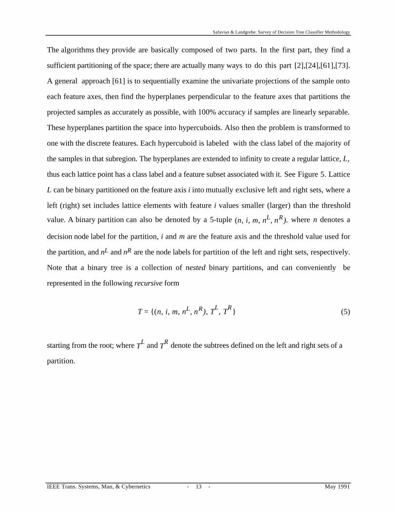
thus each lattice point has a class label and a feature subset associated with it. See Figure 5. Lattice
L can be binary partitioned on the feature axis i into mutually exclusive left and right sets, where a
left (right) set includes lattice elements with feature i values smaller (larger) than the threshold
value. A binary partition can also be denoted by a 5-tuple (n, i, m, nL, nR), where n denotes a
decision node label for the partition, i and m are the feature axis and the threshold value used for
the partition, and nL and nR are the node labels for partition of the left and right sets, respectively.
Note that a binary tree is a collection of nested binary partitions, and can conveniently be
represented in the following recursive form
T = {(n, i, m, nL, nR), TL, T
R} (5)
starting from the root; where TL and T
R denote the subtrees defined on the left and right sets of a
partition.
IEEE Trans. Systems, Man, & Cybernetics - 13 - May 1991

Safavian & Landgrebe: Survey of Decision Tree Classifier Methodology
x1
x2
ω 3 ω1
ω2
ω3
ω3
ω 3 ω3
ω1
ω1
ω 2
ω3
ω3
Figure 5. A regular lattice constructed by extending the original partitioning,with each element of the lattice assigned a class label.
For the binary trees defined on this lattice L, the general cost function considered has the form [61]
C(T) = F(L, C(TL), C(T
R)) (6)
where F(L, . , . ,) is component-wise non-decreasing and F ≥ 0. The optimization problem, is
then given L, find T* such that
C*(L) = Min C(T) = C(T*)
T(7)
The optimal tree, therefore, could be recursively constructed through the application of invariant
embedding (dynamic programing).
IEEE Trans. Systems, Man, & Cybernetics - 14 - May 1991

Safavian & Landgrebe: Survey of Decision Tree Classifier Methodology
Remarks:
1) Only one feature is examined at each node.
2) The algorithms are feasible only for a small number of features, else the size of
the lattice becomes large and storage space requirements become a problem.
This is because during the optimization process intermediate results must be
fully accessible. This perhaps is the main limitation.
The problem of designing a truly optimal DTC seems to be a very difficult problem. In fact it has
been shown by Hyafil and Rivest [39] that the problem of constructing optimal binary trees,
optimal in the sense of minimizing the expected number of tests required to classify an unknown
sample is an NP-complete problem and thus very unlikely of non-polynomial time complexity. It is
conjectured that more general problems, i.e. the problem with a general cost function or
minimizing the maximum number of tests (instead of average) to classify an unknown sample
would also be NP-complete. They also conjecture that no sufficient algorithm exists (on the
supposition that P ≠ NP) and thereby supply motivation for finding efficient heuristics for
constructing near-optimal decision trees.
The various heuristic methods for construction of DTC can roughly be divided into four categories:
Bottom-Up approaches, Top-Down approaches, the Hybrid approach and tree Growing-Pruning
approaches. In a bottom-up approach [52], a binary tree is constructed using the training set.
Using some distance measure, such as Mahalanobis-distance, pair-wise distances between a priori
defined classes are computed and in each step the two classes with the smaller distance are merged
to form a new group. The mean vector and the covariance matrix for each group are computed
from the training samples of classes in that group, and the process is repeated until one is left with
one group at the root. This has some of the characteristics of an unsupervised hierarchical
clustering approach. In a tree constructed this way, the more obvious discriminations are done
first, near the root, and more subtle ones at later stages of the tree. It is also recommended [52] that
IEEE Trans. Systems, Man, & Cybernetics - 15 - May 1991

Safavian & Landgrebe: Survey of Decision Tree Classifier Methodology
from a processing speed point of view, the tree should be constructed such that the most frequently
occurring classes are recognized first.
It is worth noting that usually most decision tree designs are restricted to having a binary structure.
This is not really a restriction since any ordered tree can be uniquely transformed into an equivalent
binary tree [65].
In top-down approaches, the design of a DTC reduces to the following three tasks:
1) The selection of a node splitting rule.
2) The decision as to which nodes are terminal.
3) The assignment of each terminal node to a class label.
Of the above three tasks, the class assignment problem is by far the easiest. Basically, to minimize
the misclassification rate, terminal nodes are assigned to the classes which have the highest
probabilities. These probabilities are usually estimated by the ratio of samples from each class at
that specific terminal node to the total number of samples at that specific terminal node. Then this is
just the basic majority rule; i.e., assign to the terminal node the label of the class that has most
samples at that terminal node.
It seems that most of the research in DTC design has concentrated in the area of finding various
splitting rules; this also naturally embodies the termination rules. Following is a summary of some
of the research done in this direction.
Wu et. al [95] have suggested that a histogram based on an interactive top-down approach for the
tree design may be especially useful for remote sensing applications. In this approach, the
histogram of the training data of all classes is plotted on each feature axis with the same scale. By
IEEE Trans. Systems, Man, & Cybernetics - 16 - May 1991

Safavian & Landgrebe: Survey of Decision Tree Classifier Methodology
observing the histograms, a threshold is selected to partition those classes into several groups. If a
group contains more than one class, the same procedure is repeated until each group contains only
one class. The drawback of this method is that only a few features (usually one) are used at each
stage. Interaction between features cannot be observed.
When the distributions of classes under consideration are known, You and Fu [97] proposed the
following approach for design of a linear binary tree classifier. Since even for moderately small
numbers of features and classes, the number of possible trees is astronomically large, they
suggested two restrictions to reduce the size of the search space. First, limit the number of features
to be used at each stage. Secondly, for the sake of accuracy, specify tolerable error probabilities at
each stage. Obviously the choice of linear classifiers and a binary tree structure is made to decrease
computational complexity and time and thus to increase the speed. Again, using a distance
measure, such as Bhattacharyya distance, classes at each node are divided into two groups. Then,
using an iterative procedure with an initial guess, a classifier is found that provides minimum
probability of error. If this error exceeds the pre-assigned error bound, the class that commits the
maximum error is taken from consideration (i.e. included in both of the following subgroups
causing overlap) and, repeating the above procedure, a new classifier is found and the error
assessed. Presuming that now the error is below the specified error bound, new subgroups are
formed, else the entire above process is repeated. Assuming that the error calculation function is
first order differentiable with respect to the coefficients of the linear equations of the classifier, they
recommended the Fletcher-Powell algorithm [19].
Remark:
Even though allowing overlap is one way of improving recognition rate, caution
must be exercised since overuse of it will cause the number of terminals to be
much larger than the actual number of classes, thus reducing the efficiency of
the tree classifier. This could be a serious drawback in large-class problems.
IEEE Trans. Systems, Man, & Cybernetics - 17 - May 1991

Safavian & Landgrebe: Survey of Decision Tree Classifier Methodology
A heuristic procedure which incorporates the time component in the tree structure design is
proposed by Swain and Hauska [77], and Wu et.al. [95]. For every node ni an evaluation
function E(ni) is defined as
E(ni) = - T(n
i) - W.e(n
i) + ∑
j=1
Ci p
i+j .E(n
i+j) (8)
where T(ni)
and e(n
i) are the computation time and the classification error associated with node
ni , respectively. W is the weighting factor, specified by the user, reflecting the relative importance
of accuracy to the computation time, and Ci is the number of descendent nodes of ni . The third
term on the right side of the above equation is the sum of the evaluation functions at the descendent
nodes of ni , weighted by their probabilities of access from ni
. Obviously in this forward top-
down search procedure, the configuration of the descendent nodes of ni is not known yet. Their
evaluation function values, however, can be lower-bound-estimated by the values of the
corresponding evaluation functions if the usual single-stage (one shot) classifier were used at ni .
The configuration that provides the maximum evaluation function among all the candidate
configurations is selected and the process is repeated at the following nodes. As pointed out in
[77], this node-by-node design approach, using only local (not global) information, can provide at
best only a suboptimal result.
Since in top-down approaches to tree design, sets of classes are successively decomposed into
smaller subsets of classes, some researchers have attempted to combine the tree design problem
and feature selection problem by using an appropriate splitting criteria at each internal node
[53],[65],[71],[73]. Rounds [65] has suggested Kolmogorov-Smirnov distance and test as the
splitting criteria. Considering a two-class problem with a binary tree structure in mind, only one
feature is selected at each internal node, with the corresponding threshold value. The rationale of
this approach is that crossover points of probability distributions of two classes (especially when
classes have multi-modal distributions) are good locations to place the partitioning planes. These
IEEE Trans. Systems, Man, & Cybernetics - 18 - May 1991

Safavian & Landgrebe: Survey of Decision Tree Classifier Methodology
crossover points also correspond to the relative maxima of difference of cumulative distributions,
also known as the Kolmogorov-Smirnov (K-S) distance. In the absence of true class distributions,
empirical distributions are estimated from the training set. The K-S distance being a random-
variable, a measure of confidence is provided by the Kolmogorov-Smirnov test. At each node for
each feature, the K-S distances and confidence level are estimated. The actual value of the feature
that provides above two maxima is used as the threshold value to create the descendant nodes.
This approach provides a means for evaluating the discrimination power and significance of each
feature in the classification process but has the following shortcomings. First of all, it requires as
many decision trees to be developed as there are pattern classes [73]. Second, this method uses
only one feature at each node. Third, even for one feature and for a two-class problem, it results in
a tree with differentiated structure and a large number of nodes. Furthermore, the K-S distance
depends on the sample sizes of both classes at each internal node, which would be in general
different at the different internal nodes. The distribution of this statistic under certain restrictions on
the relative values of sample sizes for each class can be found in Gnedenko and Kareljuk [26] and
Rounds [66].
Li and Dubes [53] proposed a permutation statistic as the splitting criterion. The permutation
statistic measures the degree of similarity between two binary vectors: the vector of thresholded
feature values, obtained from the training data, and the vector of known pattern class labels. The
advantages of this splitting criterion over, for instance, a statistic based on distance between
empirical distributions (e.g., K-S distance) are its known distribution and its independence from
the number of training patterns. Even though the permutation statistic is based on the two-class
assumption, multi-class problems can be handled by a sequence of binary decision trees.
In general, the basic idea in choosing any splitting criteria at an internal node is to make the data in
the son nodes “purer”. One way to accomplish this task [7] is to define an impurity function i(t) at
IEEE Trans. Systems, Man, & Cybernetics - 19 - May 1991

Safavian & Landgrebe: Survey of Decision Tree Classifier Methodology
every internal node t. Then suppose that for the internal node t there is a candidate split S which
divides node t into left son tL and right son tR such that a proportion pL of the cases in t go into tL
and a proportion pR go into t
R. One could then define the goodness of the split S to be the
decrease in impurity
∆i(S,t) = i(t) - i(tL)p
L - i(t
R)p
R (9)
Then choose a split that minimizes ∆i(S,t) over all splits S in some set S . The impurity function
suggested in [7] is the Gini index defined as
i(t) = ∑i≠j
p(i| t)p(j| t) (10)
where p(i| t) is just the probability of a random sample X_ belonging to the the class i, given we are
at node t.
The final component in top-down DTC design is to determine when the splitting should be
stopped; i.e., we need a stopping rule. Early approaches to selecting terminal nodes were of the
form: set a threshold β > 0 and declare a node t terminal if
max ∆i(S(t), t) < βS∈S
(11)
The problem with this rule is that usually partitioning is halted too soon at some nodes and too late
at some others. The other major problem in deciding when to terminate splitting is the following.
Suppose we have classes whose underlying distributions overlap; that is the true misclassification
rate is positive ( R*(d) > 0). Furthermore, suppose we have a training set L, and we use a splitting
approach (e.g. impurity function) along with a terminal labeling approach mentioned earlier, and
continue the splitting until every node has pure samples; i.e., samples from only one class. Now
IEEE Trans. Systems, Man, & Cybernetics - 20 - May 1991

Safavian & Landgrebe: Survey of Decision Tree Classifier Methodology
consider the resubstitution estimate (see III, definition 15) of the misclassification rate of the tree T
defined as
R(T) = ∑t∈∼
T
r(t)p(t) = ∑t∈∼
T
R(t) (12)
where r(t) is the resubstitution estimate of the misclassification rate, given a sample falls into node
t, p(t) is the probability of a random sample falling into node t, and ∼T is the set of terminal nodes
of the tree T. Notice that for above scenario R(T) = 0! Obviously this estimate is very biased. That
is, in general, R(T) decreases as the number of terminal nodes increases. But the tree so
constructed usually fails miserably in classification of the test data. Breiman, et.al. [7] conjectured
that decision tree design is rather insensitive to a variety of splitting rules, and it is the stopping rule
that is crucial. Breiman et.al. [7] suggest that instead of using stopping rules, continue the splitting
until all the terminal nodes are pure or nearly pure, thus resulting in a large tree. Then selectively
prune this large tree, getting a decreasing sequence of subtrees. Finally, use cross-validation to
pick out the subtree which has the lowest estimated misclassification rate. To go any further, we
need the following definitions (see [7] for more detail).
Definitions:
16) A branch Tt of tree T with root node t∈T consists of node t and all the
descendants of t in T.
17) Pruning a branch Tt from a tree T consists of deleting from T all descendants
of t. Denote the pruned tree as T- Tt.
18) If by successively pruning off branches from T we obtain the subtree T', we
call T' a pruned subtree of T and denote it by T'< T.
Recall that the size of a tree is of utmost importance. In order to include the complexity of tree T in
the design process, define a cost-complexity measure Rα(T) as
IEEE Trans. Systems, Man, & Cybernetics - 21 - May 1991

Safavian & Landgrebe: Survey of Decision Tree Classifier Methodology
Rα(T) = R(T) + α | ∼T | (13)
where R(T) has the usual meaning of estimated misclassification rate of tree T , and α >= 0 is the
complexity cost measure. That is, the complexity of tree T is measured by the number of its
terminal nodes, and α is the complexity cost per (terminal) node. Let us denote the fully grown tree
as Tmax. Then the objective of a pruning process is, for every α , find the subtree T (α) <= Tmax
such that
Rα(T(α)) = min Rα(Τ) T <= Tmax
(14)
Notice that as α is varied from sufficiently small values where Tmax itself is the optimally pruned
tree, to sufficiently large values where Tmax is pruned so far that only the root node {root} is left,
one obtains a finite sequence of trees T1, T
2, ..., {root}; where T
i corresponds to the optimal
subtree for α = αi. Then among these trees, the tree that provides the smallest test sample or
cross-validation estimate of the misclassification rate is selected. (See [7] for more details.)
Note that the pruning algorithm is essentially a (multipass) top-down algorithm. The tree growing
and pruning of Breiman et.al. [7] has been incorporated into a computer program known as CART
(Classification and Regression Trees.) Following are some of the shortcomings of CART. First of
all, CART allows only either a single feature or a linear combination of features at each internal
node. Second, CART is computationally very expensive as it requires generation of multiple
auxiliary trees. Finally and perhaps most importantly, CART selects the final pruned subtree from
a parametric family of pruned subtrees, and this parametric family may not even include the optimal
pruned subtree. There are, of course, other tree growing and, more importantly, pruning
algorithms (e.g. [12],[25]). Gelfand et.al. [25] propose an iterative tree growing and pruning
algorithm based on the following ideas:
IEEE Trans. Systems, Man, & Cybernetics - 22 - May 1991

Safavian & Landgrebe: Survey of Decision Tree Classifier Methodology
1) Divide the data set into two approximately equal sized subsets and iteratively
grow the tree with one subset and prune it with the other subset.
2) Successively interchange the role of the two subsets.
Their pruning algorithm is a simple and intuitive one-pass bottom-up approach which starts from
the terminal nodes and proceeds up the tree, pruning away branches. They prove the convergence
of their algorithm, and their experimental results on waveform recognition, along with the
theoretical proof, suggests the superiority of their algorithm to the pruning algorithm of Breiman
et.al.[7]. (See [25] for details.)
Recently, a hybrid method was proposed by Kim and Landgrebe [41] that uses both bottom-up
and top-down approaches sequentially. The rational for the proposed method is that in a top-down
approach such as hierarchical clustering of classes, the initial cluster centers and cluster shape
information are unknown. It is also well known that the proper choice of initial conditions could
considerably influence the performance of a clustering algorithm (e.g., speed of convergence and
final clusters). These information can be provided by a bottom-up approach. The procedure is as
follows. First, considering the entire set of classes, one uses a bottom-up approach such as [52] to
come up with two clusters of classes. Then one computes the mean and covariance for each cluster
and uses these information in a top-down algorithm such as [95] to come up with two new
clusters. Every cluster is checked to see if it contains only one class. If so, that cluster is labeled as
terminal; else the above procedure is repeated. The procedure terminates when all the clusters are
labeled as terminals. (See [41] for details.)
In all the foregoing discussions, at each node a decision is made and only one path is traversed
from the root of the tree to a terminal node. This is referred to as a "hard-decision system" by
IEEE Trans. Systems, Man, & Cybernetics - 23 - May 1991

Safavian & Landgrebe: Survey of Decision Tree Classifier Methodology
Schuerman and Doster [68]. In contrast to hard-decision systems, they propose an approach where
all the a posteriori probabilities are approximated at each internal node without making a decision at
any of those points; a decision is made only at the terminal nodes of the tree by selecting the
maximum a posteriori probability. In other words, in a manner similar to single-stage approaches
[23], a posteriori probabilities for the different classes are estimated, but in a sequence of steps.
Obviously, one would expect to obtain the same a posteriori probabilities at the terminal nodes as
the ones the global single stage classifier would give, assuming the estimated a posteriori
probabilities at each internal node are the same as the actual values.
In single-stage classifications, one way to classify an unknown sample into one of m classes is to
evaluate (m-1) discriminant functions [18],[23]. When Bayes minimum probability of error is the
desired criterion, these discriminant functions are the a posteriori probabilities. In a sequential
approach to evaluate these probabilities, the conditional probabilities of classes at each of the output
branches of an internal node are estimated, based on the set of classes and the full feature
measurement vector at the input to that node. Obviously the structure of the tree and the accuracy of
these estimates are somewhat related. But, clearly, if the true a posteriori probabilities could be
furnished, the explicit structure of the tree would not be critical. So, at least conceptually, the input
classes at each node can be decomposed in a way that a posteriori probabilities of the classes at the
outgoing branches may be estimated with "maximal confidence." Again due to the enormous
number of possible combinations at each node, the actual tree is usually constructed using training
data and heuristic methods based on a separability measure.
Mean square polynomial discriminant functions, using training sets, are suggested [96] for
estimating the a posteriori probabilities of classes at the output of each node branch given the set of
classes at the input of the node and the full feature measurement vector.
Remarks:
IEEE Trans. Systems, Man, & Cybernetics - 24 - May 1991

Safavian & Landgrebe: Survey of Decision Tree Classifier Methodology
1) By thresholding these a posteriori probabilities at each node, if desired, the
soft-decision approach can be converted to the conventional hard-decision
approach.
2) When the number of classes is large and no overlap is allowed in the tree, the
hard-decision approach raises the possibility of error accumulation [81]-[83].
Even though using heuristics such as proper tree search strategies (see section
IV.3) this error can be reasonably controlled [81], but the soft-decision
approach avoids the problem altogether.
3) When the number of classes and features are large and the class distributions
have significant overlap, a hard-decision approach usually covers up
ambiguities by a "forced recognition" [68]. In the soft-decision approach, no
decision is made until the last stage of the tree.
4) In general, however, the computational time complexities of the soft-decision
approach may be a limiting factor.
IV.1.b. ENTROPY REDUCTION AND INFORMATION-THEORETIC APPROACHES
A different point of view about pattern recognition is taken by Watanabe [85]-[93] and Smith and
Grandy [75]. Since organization and structure of objects or a set of stochastic variables could be
expressed in terms of entropy functions [86], Watanabe refers to the problem of pattern recognition
as that of "seeing a form" or structure in an object [86], and he suggests ways to cast the problems
of learning [88],[89], such as feature (variable) selection, dimensionality reduction [91], and
clustering [90],[92], to mention a few, in terms of minimizing properly defined entropy functions.
IEEE Trans. Systems, Man, & Cybernetics - 25 - May 1991

Safavian & Landgrebe: Survey of Decision Tree Classifier Methodology
As noted by Suen and Wang [76],[81] this point of view could be very attractive when the number
of classes is large and calculation of Bayes error probabilities is not so simple. Basically, since at
the root of a tree, a given sample could belong to any of the classes, the uncertainty is maximum.
At the terminal nodes of the tree, the sample is eventually classified and the uncertainty is
eliminated. So, an objective function for a tree design could be to minimize uncertainty from each
level to the next level, or in other words, maximize entropy reduction at each stage. Since it is also
desirable to have as few overlaps as possible, Suen and Wang [76] suggested an interactive
iterative clustering algorithm (ISOETRP) with an objective function directly proportional to the
entropy reduction and inversely proportional to some function of class overlap at each stage of the
tree. Even though any entropy measure could be used, Shannon's entropy, defined as
H = - ∑i
pi log p
i (15)
where pi is the a priori probability of class i, is preferred because of its strong additivity property
[1].
Sethi and Sarvarayudu [73] propose a simple, yet elegant, method for the hierarchical partitioning
of the feature space. The method is non-parametric and based on the concept of average mutual
information. More specifically, let the average mutual information obtained about a set of classes
Ck from the observation of an event X
k, at a node k in a tree T be defined as
Ik(C
k; X
k) = ∑
Ck
∑X
k
p(Cki
, Xkj
). log2[
p(Cki
)
p(Cki
| Xkj
) ]
(16)
Event Xk represents the measurement value of a feature selected at node k and has two possible
outcomes; measurement values greater or smaller than a threshold associated with that feature at
that node.
IEEE Trans. Systems, Man, & Cybernetics - 26 - May 1991

Safavian & Landgrebe: Survey of Decision Tree Classifier Methodology
Then, the average mutual information between the entire set of classes, C, and the partitioning tree,
T, can be expressed as
I(C; T) = ∑k=1
L p
k. I
k(C
k; X
k)
(17)
where pk is the probability of the class set Ck
and L is the number of internal nodes in the tree T.
The probability of misclassification, pe , of a decision tree classifier T and the average mutual
information I(C; T) are also related as [73]
I(C; T) >- - ∑j=1
m[p(C
j). log
2p(C
j)] + pe. log
2pe + (1-pe).
log2(1-pe) + pe. log
2(m-1)
(18)
with equality corresponding to the minimum required average mutual information for a pre-
specified probability of error. Then a goal for design of the tree could be to maximize the average
mutual information gain (AMIG) at each node k. The algorithm terminates, when the tree average
mutual information, I(C;T), exceeds the required minimum tree average mutual information
specified by the desired probability of error. (See [73] for more details.) An alternative stopping
criterion proposed by Talmon [78] is to test the statistical significance of the mutual information
gain that results from further splitting a node.
A tree constructed by this top-down algorithm would have a binary structure, and since at each
node the partitioning hyperplane (i.e., the optimum feature and its corresponding threshold) is
selected to maximize the average mutual information at that node, the performance is optimized in a
"local sense". Once the partitioning is specified, the globally optimum tree could be obtained using
the algorithm suggested by Payne and Meisel [61].
IEEE Trans. Systems, Man, & Cybernetics - 27 - May 1991

Safavian & Landgrebe: Survey of Decision Tree Classifier Methodology
Chou and Gray [11] view decision trees as variable-length encoder/decoder pairs, and compare the
performance of the decision trees to the theoretical limits given by the rate-distortion function.
More specifically, they show that rate is equivalent to the average tree depth while the distortion is
the probability of misclassification. They also use greedy algorithms to design trees and compare
their performances to certain classes of optimal trees under certain restrictive conditions. The
applicability of their method is limited, in practice, to only small problems. Goodman and Smyth
[29] prove that a tree designed based on a top-down mutual information algorithm is equivalent to a
form of Shannon-Fano prefix coding. They drive several fundamental bounds for mutual
information-based recursive tree design procedures. They also suggest a new stopping rule which
they claim to be more robust in the presence of noise.
When the measurement variables (features) are discrete, as for instance, in computer diagnostics of
diseases or in stroke directions or number of line crossings in character recognition, the
conventional classifier design or feature selection techniques face practical difficulties [71]. This is
mainly due to the non-metric nature of the measurement space. Sethi and Chatterjee [71] use
concepts of prime events to come up with an efficient approach to the decision tree design. Even
though their method does not guarantee optimality, in most cases it provides close to optimal
results, but most importantly, it is efficient.
IV.2. FEATURE SELECTION IN DTC'S
Regardless of its importance, the problem of feature subset selection in DTC's has received
relatively little attention. Kulkarni and Kanal [46] proposed the use of a branch-and-bound
technique [51] to assign features to the nodes in a sequential top-down manner. The probability of
error is calculated for each possible feature subset selected; if it exceeds the pre-assigned lower
bound then that feature subset is abandoned.
IEEE Trans. Systems, Man, & Cybernetics - 28 - May 1991

Safavian & Landgrebe: Survey of Decision Tree Classifier Methodology
Due to computation time, as a practical matter, the size of the feature subset to be used at each node
is usually limited to be much smaller than the total number of available features [97]. Once it has
been determined (often heuristically) how many features are to be used at each node, different
feature subsets are examined and the one that provides maximum separability, measured by some
distance function, among classes accessible from that node, is usually selected. Note that when the
number of classes is large, an exhaustive search may be infeasible. In that case, usually a greedy-
type search algorithm is used. Again, this at best would provide local optimality. Some studies, in
order to determine the significance of each feature in discriminating among classes associated with
each node, have offered methods that utilizes only one feature at each node. It should be noted that
while the use of single feature decisions at every internal node reduces the computational burden at
the tree design time, it usually leads to larger trees.
Recently, the subject of neural networks, has become very popular in many areas such as signal
processing and pattern recognition. Actually, the applications of neural networks in pattern
recognition problems go back to the days of simple perceptrons in the 1950'S. Many advantages
for neural networks have been cited in the literature (c.f. Rumelhart et.al. [67] and Lippmann
[55]). Most important of them, for the pattern recognition problems, seems to be the fact that
neural network-based approaches are usually nonparametric even though statistical information
could be possibly incorporated to improve their performance (speed of convergence, etc.). Also
neural networks can extract nonlinear combinations of features, and the resulting discriminating
surfaces can be very complex. These characteristics of neural networks can be very attractive in a
decision tree classifier where one has to determine the appropriate feature subsets and the decision
rules at each internal node. There are various neural network models such as Hopfield nets, the
Boltzmann machine and Kohonen self-organizing feature maps, to name a few; the most popular
network by far, however, is the multilayer feedforward network [67].
IEEE Trans. Systems, Man, & Cybernetics - 29 - May 1991

Safavian & Landgrebe: Survey of Decision Tree Classifier Methodology
A multilayer feedforward neural network is simply an acyclic directed graph consisting of several
layers of simple processing elements known as neurons. The neurons in every layer are fully
connected to the neurons in the proceeding layer. Every neuron sums its weighted inputs and
passes it through some kind of nonlinearity, usually a sigmoidal function. The first layer is the
input layer, the last layer is the output layer and the intermediate layers are known as the hidden
layers. See Figure 6. Then for a supervised learning, training samples are assigned to the inputs of
the network, and the connection weights between neurons are adjusted such that the error between
the actual outputs of the network and the desired outputs are minimized. A commonly used error
criterion is the total sum-of-squared error between the actual outputs and the desired outputs. There
are many learning algorithms to perform this learning task; a frequently used learning rule is the
back propagation algorithm which is basically a (noisy or stochastic) gradient descent optimization
method. Note that, once one fixes the structure of the network, i.e., the number of hidden layers
and the number of neurons in each hidden layer are chosen, then the network adjust its weights via
the learning rule until the optimum weights are obtained. The corresponding weights (along with
the structure of the network) create the decision boundaries in the feature space. The question of
how to choose the structure of the network is beyond the scope of this paper and is a current
research issue in neural networks. It suffices to mention that for most practical applications,
networks with only one hidden layer are utilized. Also see comments in section V and [55].
IEEE Trans. Systems, Man, & Cybernetics - 30 - May 1991

Safavian & Landgrebe: Survey of Decision Tree Classifier Methodology
Input Layer Hidden Layer Output Layer
α 11β
11
x1
x2
x6
y1
y2
y3
Figure 6. A three layer feedforward network with 6 inputs and 3 outputs. αij and
βkl are the connection weights between neuron i of input layer and neuron j of
hidden layer and neuron k of hidden layer and neuron l of output layer,
respectively.
How can neural networks assist us in the design of decision trees? Gelfand and Guo [31] propose
the following. Recall that in every internal node t of the tree T one would like to find the optimum
(here, in the local sense) feature subset and the corresponding decision surface to partition C(t), the
set of classes in t, into C( tL) and C( tR), two subset of classes at nodes tLand tR, respectively. That
is, there are two nested optimization tasks involved here. The outer optimization loop searches for
the optimum partitioning of classes into two (possibly disjoint) subsets of classes and the inner
optimization loop searches for the optimum decision surface in the feature space to perform the
outer optimization task. Suppose for now that we know the partitioning of C(t) into C( tL) and
C( tR), and are only looking for the (optimum) decision surface in the feature space. This, of
course, can be easily implemented by a simple multilayer feedforward network. Then the
remaining question is how to partition C(t) into C( tL) and C( tR)? As mentioned in section IV.1,
there are various splitting rules. One such possible rule is the impurity reduction criterion used in
IEEE Trans. Systems, Man, & Cybernetics - 31 - May 1991

Safavian & Landgrebe: Survey of Decision Tree Classifier Methodology
CART. That is, one will consider various partitioning of the C(t) into C( tL) and C( tR), and choose
the partitioning that gives the maximum impurity reduction (see section IV.1.a, and [7] for details).
Of course, when the number of classes is large, an exhaustive search may be impractical. In this
case, some type of greedy search can be performed.
IV.3. DECISION RULES AND SEARCH STRATEGIES IN DTC's
Once the tree structure is designed and the feature subsets to be used at each node of the tree are
selected, a decision rule is needed for each node. These decision rules could be designed such that
optimal performance (in any specified sense) could be attained at each node (i.e. local optimality);
or the overall performance of the tree could be optimized (i.e. global optimality). Obviously,
decision strategies designed to provide optimum performance at each node, do not necessarily
provide overall optimum performance. For globally optimum performance, decisions made at each
node should "emphasize the decision which leads to a greater joint probability of correct
classification at the next level" [50]; i.e., decisions made at the different nodes are not independent.
Kurzynski [49],[50] addresses both locally and globally optimum decision rules. He shows that
the decision rule that provides minimum probability of error at each node (i.e., local optimality) is
just the well known maximum a posteriori probability rule. Since for globally optimum rules, error
recognition information in the future nodes are needed, the problem is worked in a sequentially
backward (bottom up) manner starting from the terminal nodes.
Let us assume that there are m pattern classes and λij represents the cost or losses incurred in
classifying a sample from class Ci to class Cj. Then the Bayes minimum risk classifier allocates an
unknown pattern sample to class Ck if
k = arg ( min ∑i=1
m p(C
i | X) λ
ij )
j (19)
IEEE Trans. Systems, Man, & Cybernetics - 32 - May 1991

Safavian & Landgrebe: Survey of Decision Tree Classifier Methodology
where X is the feature measurement vector of the unknown sample. For a "0-1" loss function, λij =
1-δij where δij is the Kronecker delta. Then, above rule becomes the simple maximum a posteriori
rule, i.e.,
C
k = arg ( max p(C
i | X ) )
i(20)
Even though "0-1" is a reasonable and frequently used loss function, in a decision tree classifier, it
should only be applied at the terminal nodes where the actual classification task is performed. At
the intermediate nodes in a tree, decisions are made as to which of the possible branches leaving
that node should be followed. Let αij represent the cost incurred when a sample of class Ci is
routed through branch j. Obviously, αij is a random variable since (Dattatreya and Kanal [13])
actions at the levels below the present level are not known. Dattatreya and Kanal [13] propose an
interesting unsupervised scheme that adaptively learns the mean values of these random variables
and improves the tree performance.
The only cost considered above was the cost of decision-making and classification. What about the
cost of feature measurements? In many applications, such as medical diagnosis, feature
measurement costs (e.g., lab tests, X-rays, and etc.) may be a major portion of the cost. Thus
more generally, the total cost should be (Dattatreya and Sarma [16], and Kulkarni and Kanal [45])
the sum of the feature measurement cost and the classification cost. Assuming that feature
measurement costs are constant, Wald [80] shows that the minimum cost classifier is a multistage
scheme which measures only one feature at every stage and decides the next course of action.
Furthermore, Dattatreya and Sarma [16] show that rejection of class labels at intermediate stages as
unlikely candidates is suboptimal in the Bayes minimum cost sense.
Now consider the situation where the tree is designed and feature subsets to be used at each node
are determined. In this case, the problem of hierarchical classification can also be viewed as a
problem of tree search. Kanal [40], and Kulkarni and Kanal [46] have generalized the idea of state
IEEE Trans. Systems, Man, & Cybernetics - 33 - May 1991

Safavian & Landgrebe: Survey of Decision Tree Classifier Methodology
space representation and ordered admissible search methods of Artificial Intelligence (Nilsson [60])
to the problem of hierarchical classification. Then, to search through the tree, an evaluation
function f(n) (Kanal [40]) is defined at each node n as
f (n) = g(n) + h(n) + l(n) (3.16)
where g(n) is the cost from the root to node n, h(n) is (an estimate of) the cost from n to a
terminal node accessible from n, and l(n) is (an estimate of) the risk of classification at a terminal
node accessible from n.
At a goal node, s*, the total cost is the sum of measurement costs at each node along the path from
the root to s* plus the actual risk, r(s*), associated with s*. If r(s*) is estimated based on only the
feature measurements at each node along the path from the root to s*, the strategy that provides
minimum total cost is called an S-admissible search strategy. When r(s*) is estimated using all the
measurements, not just those on the path to s*, then the strategy that provides minimum total cost
is known as a B-admissible search strategy (Kanal [40]).
At every node, a lower bound on the value of risk is used in the evaluation function for the S-
admissible search, except for a goal node where the actual risk is used. In a B-admissible search,
however, since the risk associated with any goal s* can change as additional measurements are
made along other paths in the tree, a search could not be terminated simply as one goal state is
reached. Therefore, an upper bound function on the risk is also needed to determine the termination
point (Kanal [40], and Kulkarni and Kanal [46]). Obviously, the performance of either of the
above two search methods is dependent on one's ability to find proper bounds on the goal risk.
The advantage of the state-space model as pointed out by Kulkarni and Kanal [46] is that, in
contrast to the hierarchical classifier approach where only one path is pursued from the root to a
terminal point, here provisions are made to back up and follow other alternative paths in the tree if
IEEE Trans. Systems, Man, & Cybernetics - 34 - May 1991

Safavian & Landgrebe: Survey of Decision Tree Classifier Methodology
it is needed. Obviously, however, this would increase the number of nodes visited before a
decision is made and thus reduce the efficiency. Also search efficiency is a function of the tightness
of the bounds on the risk; and tight bounds are difficult to obtain particularly for some continuous
distributions [46]. It is also interesting to note that the way cost functions are usually defined
neither the B-admissible nor the S-admissible search has provisions for the time component [81].
As mentioned earlier, when the number of classes is large, i.e. on the order of hundreds or even
thousands as is in the Chinese character recognition problem for instance, tree classifiers could
provide a considerable amount of time savings. But error has a tendency to accumulate from level
to level. This is because in problems with large numbers of classes, the tree has many levels. If e
is the minimum error at each node of each level and there are on the average l levels in the tree, the
average total error rate of the tree would be on the order of (l * e). As proposed in Wang and
Suen [81], there are two ways to reduce the total error: either reduce e or have a better search
strategy capable of backing-up and re-routing. In general e can only be reduced by allowing
overlaps at internal nodes [95]; but this would increase the number of nodes and terminal nodes,
thus greatly increasing the memory space requirements. To improve tree search, however, several
heuristic search strategies are proposed [2],[9],[10],[28],[33],[35],[81]-[83]. Chang and Pavlidis
[10] proposed a branch-bound-backtracking algorithm. A fuzzy decision function [99], taking
values in the interval [0,1], is used to assign the decision values of all the branches going out of a
node. The overall decision value of a path is defined to be the product of the decision values of all
the branches along that path. The product operator could be either the regular product or the max-
min operator [9]. Branches with the largest decision values are followed. At any node, if the total
decision value up to that node falls below a pre-specified threshold, the algorithm backtracks to the
previous node(s) and follows another path. Of course, the speed of the search is related to the
threshold value set.
IEEE Trans. Systems, Man, & Cybernetics - 35 - May 1991

Safavian & Landgrebe: Survey of Decision Tree Classifier Methodology
Since the most confusion and error occurs for samples that come from regions near the boundaries
between classes (or groups of classes), Wang and Suen [81] propose a two-step search approach.
In the first step, following the usual top-down search approach, an unknown sample reaches a
terminal node. The degree of similarity of the sample with the class label associated with that node
is computed. If this value is above a preset threshold, the sample is classified and the next sample
is treated; otherwise, the unknown sample goes through the second search called "fuzzy logic
search." As argued in [81], the rationale for fuzzy logic is that somehow the global search
information and all the possible terminals (classes) must be recorded. Probabilistic decision values
based on Bayes decision regions, although perhaps more precise, are usually much harder to
estimate. Fuzzy decision values, however, are both flexible and easier to compute. By adjusting
the two thresholds involved in the two steps, the speed of the search could be controlled. This
would also provide a trade-off between speed and accuracy of the tree classifier.
V. OTHER TREE RELATED ISSUES
A) Incremental tree design:
With regard to the training samples, there are two possibilities: 1) The entire training sample is
available at the time of decision tree design; 2) the training sample arrives in a stream.
For case 1, once a tree is designed the task is completed and such design algorithms are known as
non-incremental algorithms. For the second case, however, one has two options:
a) Whenever the new training samples become available, discard the current tree
and construct a replacement tree using the enlarged training set.
b) Or revise the existing tree based on the new available information.
Procedures corresponding to b) are known as incremental decision tree design algorithms.
IEEE Trans. Systems, Man, & Cybernetics - 36 - May 1991

Safavian & Landgrebe: Survey of Decision Tree Classifier Methodology
Of course, it would be desirable that the incremental decision tree design algorithms produce the
same trees as those if all the training samples were available at the time of design. Utgoff [79] has
developed one such incremental algorithm.
B) Tree generalization:
In designing a DTC, one must always keep in mind that the tree designed is going to be used to
classify unseen test samples. With this in mind, one has two options: 1) Design a decision tree that
correctly classifies all the training samples, also known as a perfect tree [62],[63]; and select the
smallest perfect tree. 2) Or construct a tree that is perhaps imperfect (in the above sense) but has the
smallest possible error rate in classification of test samples. In practical pattern recognition tasks, it
is usually this second type of tree that is of most interest.
Regardless of which of the above two types of trees one may need, it is usually desirable to keep
the size of the tree as small as possible. The reasons for this are: 1) Smaller trees are more efficient
both in terms of tree storage requirements and test time requirements; 2) smaller trees tend to
generalize better for the unseen samples because they are less sensitive to the statistical
irregularities and idiosyncrasies of the training data.
C) Missing value problem:
The missing value problem can occur in either the design phase, or the test phase, or both. In the
design step, suppose some of the training sample feature vectors are incomplete; that is some
feature elements of some feature vectors are not recorded or are missing. This can happen, for
instance, due to some occasional sensor failures. Similarly for the test samples, some feature
values may be missing.
IEEE Trans. Systems, Man, & Cybernetics - 37 - May 1991

Safavian & Landgrebe: Survey of Decision Tree Classifier Methodology
In the design phase, one simple but wasteful method to cope with this problem is to throw away
the incomplete feature vectors. For the test sample, of course, this simple option is not acceptable.
Breiman et.al. [7] propose the following solution which is based on the idea of using surrogate
splits. For the case of simplicity, consider the case of binary splitting at every internal node based
on the value of only one feature. For the extension of this idea to a linear combination of features,
see [7] and [21]. The basic idea is as follows.
In the tree design phase, at node t, find the best split Sm* on the feature element X musing all the
training samples containing a value of X m. Then select the split S* which maximizes the impurity
reduction ∆i (Sm* , t) at node t (see section IV 1.a) .
For the incomplete test sample, if at a node t the best split S* is not defined because of missing
feature element values, proceed as follows. Define a measure of similarity between two splits
Si and Sj as λ( Si ; Sj ) . Examine all non-missing feature elements for the test sample; find that
one, say X m, with split ∼Sm , that is most similar to S* . ∼Sm is called a surrogate split to S* . Then
use ∼Sm at node t to decide to traverse to node tL or tR.
D) Robustness of decision tree design:
Since decision trees are often constructed by using just some sets of training samples, it is
important to make sure that the design procedure is in some sense robust relative to the presence of
"bad" samples or outliers. Of course, one could always edit the training data before application in
the tree design. This, however, in many cases may not be feasible for the following reasons.
1) The designer may not be aware of the existence of outliers at the time of the tree design,
even though outliers are usually easily detected in a training set; in some cases a thorough
examination of data set may be necessary.
IEEE Trans. Systems, Man, & Cybernetics - 38 - May 1991

Safavian & Landgrebe: Survey of Decision Tree Classifier Methodology
2) With a small sample, one may not want to throw away any valuable samples.
E) Decision trees and neural networks:
Even though multilayer perceptron (MLP) networks and DTC's are two very different techniques
for classification, the similarities in the distributed nature of decision-making in both processes has
motived some researchers [5] to perform some empirical comparative studies. Following are some
of the general conclusions drawn so far.
1) Both DTC's and MLP networks are capable of generating arbitrarily complex decision
boundaries from a given set of training samples; usually neither needs to make any assumptions
about the distributions of the underlying processes.
2) MLP networks are usually more easily capable of providing incremental learning than
DTC's.
3) Training time for MLP networks is, however, usually much longer than the training time
for DTC's. Therefore, MLP networks tend to be most useful in the circumstances where the
training is infrequent and the given classifier is used for a long period of time.
4) In the empirical studies reported in [5], MLP networks performed as well as or better
than their CART counterpart.
5) DTC's are sequential in nature, compared to the massive parallelism usually present in
MLP networks.
6) The behavior of DTC's in general, and CART in particular, make it much more useful
for data interpretation than MLP networks. An MLP network, in general, is no more than a black
box of weights; and reveals little information about the problem its applied to.
7) Perhaps the most interesting conclusion in [5] is that there is not enough evidence
(theoretical or empirical) to provide a strong support for either one of the approaches alone.
IEEE Trans. Systems, Man, & Cybernetics - 39 - May 1991

Safavian & Landgrebe: Survey of Decision Tree Classifier Methodology
Then, perhaps a more useful stand to take with regards to the decision trees and neural networks is
to consider both of these tools together. This may be looked at from following two perspectives.
I) Neural networks may be used in the implementation of various aspects of decision trees.
For instance, Gelfand and Guo [31] use neural networks in the internal nodes of a decision tree to
perform the task of feature selection and decision boundary construction. In this approach, one is
constructing a tree of neural networks. See also Golea and Marchand [27]
II) The alternate possibility is to design the DTC and then map the tree into a neural
network. This is the direction Sethi [69]-[70], and Sethi and Otten [72] have taken. The main idea
here is that, as it was mentioned earlier in section IV.2, in the design of multilayer feedforward
networks, the structure of the network, i.e., the number of hidden layers and the number of
neurons in each hidden layer is not known in advance, and is often chosen rather heuristically and
by trial and error. The method described in [69], [70], and [72] offers one way to uncover the
structure of the network. That is, they offer a method to implement a pre-designed decision tree via
a multilayer feedforward neural network. Perhaps one of the main advantages of this approach,
other than possibly eliminating guess work in the design of MLP networks, is that the network
designed this way usually has fewer connections. This may be an important factor from VLSI
implementation point of view.
VI. CONCLUSIONS AND FINAL REMARKS
Decision tree classifiers show a great deal of potential in many pattern recognition problems such
as remotely sensed multisource data classification, medical diagnosis, speech and character
recognition, to mention a few. Perhaps one of the main features of DTC's is the flexibility they
provide; for example the capability of using different feature subsets and decision rules at different
IEEE Trans. Systems, Man, & Cybernetics - 40 - May 1991

Safavian & Landgrebe: Survey of Decision Tree Classifier Methodology
stages of classification and the capability of trade-offs between classification accuracy and
time/space efficiency.
Some of the goals of this review have been to:
1) Bring the disparate issues in decision tree classifiers closer together and
perhaps motivate some new ideas;
2) Provide a more unified view of decision tree classifiers;
3) And caution the "casual" users of these methods of the possible "pitfalls" of
each method.
Even though optimization techniques such as dynamic programing have been offered by some
researchers to define trees that have certain optimal characteristics, a practical and feasible solution
that is truly optimal with respect to the choice of tree structure, feature subsets and decision rule
strategies is yet far from realization. This is mainly due to either unavailability of the necessary
information (e.g., a priori and class conditional statistics) for the design or to complexities of the
proposed methods that limits their usefulness for real applications of moderate or large size.
Recognizing the difficulties involved in the design of optimal DTC's, many heuristic methods have
been proposed in the literature.
The four basic approaches for design of DTC's examined in this review are:
1) Bottom-up approach where one starts with the information classes and
continues combining classes until one is left with a node containing all the
classes (i.e., the root).
IEEE Trans. Systems, Man, & Cybernetics - 41 - May 1991

Safavian & Landgrebe: Survey of Decision Tree Classifier Methodology
2) Top-down approach where starting from the root node, using a splitting rule,
classes are divided until a stopping criterion is met. The main issues in this
approach are: a) choice of splitting criterion; b) stopping rules ; c) labeling the
terminal nodes.
3) Hybrid approach where one use a bottom-up procedure to direct and assist a
top-down procedure.
4) Tree growing-pruning approach where in order to avoid some difficulties in
choosing a stopping rule, one grows the tree to its maximum size where the
terminal nodes are pure or almost pure, and then selectively prunes the tree.
As was pointed out earlier, computational efficiency, accuracy of classification and storage space
requirements usually seem to be conflicting requirements. This fact may actually assist the designer
(user) of a DTC in selecting one possible scheme over the others. The existing methods with their
relative time/space complexities, degrees of (sub)optimality and proposed areas of applications are
summarized in the following tables. Table 1 provides a summary of some of the tree design
methods in terms of the assumptions each approach makes, their performance criterion and some
of the specific requirements of each method. Table 2 gives the brief summary of various feature
selection methods. Table 3 summarizes the various decision rule and search strategies used in
decision trees. And finally, Table 4 provides specific references for various applications.
Finally it should be pointed out that since the performance of a DTC depends on how well the tree
is designed, special attention should be paid to this phase. In particular, when the number of test
samples to be classified is large, as is, for example, in remote sensing applications, the time spent
for the design could be well justified.
IEEE Trans. Systems, Man, & Cybernetics - 42 - May 1991

Safavian & Landgrebe: Survey of Decision Tree Classifier Methodology
Table 1 - Summary of tree structure design
Ref. Optimal ? Criterion Assumptions Remarks(by author or alternate ref.)
4 Locally(node-wise)
Prob. of error- Given: a well
defined featuretransformation
- An automated technique;- uses only a priori statistics;- a procedure to compute the global Pe
is also provided.
8 No Max.inf.gainat each node.
- Given: a binaryimage with apriori classprob.'s;
- and number ofblack bits ineach position ineach class inthe designsamples.
-Input (for classification) is a 2-Dbinary pattern
- computationally efficient;- storage requirements reasonable;- especially suited for (optical)
character recognition.
15 YesMin. total cost(feature meas.cost + classif.
cost).
- Designsamplesavailable;
- conditionaldensities areunimodal.
-Provides a binary tree;-superior performance to the method
proposed in ref. #13; both in termsof simplicity of design and the totalexpected cost of classification.
16 No " –-Heuristic;- provides a binary tree.
45 YesWeighted sumof Pe and avg.meas. cost inclassifying arandom sample
- Uses ML ateach node
- overall Pe oftree is small;
- features on anypath from rootto a terminalnode are statist.indep
- A bottom-up approach;-time and space complexities are high.
52 No – - Training sampleavail.
- Unsupervised clustering of a prioriclasses.
53 No Accuracy- Labeled training
patternavailable.
- Examines 1 feature at each node;- finds best feature and corresp.
threshold for each node.
57 Yes A general costfunction.
- Given: samplesfrom all theclasses.
- Binary tree;- storage requirements may be large.
IEEE Trans. Systems, Man, & Cybernetics - 43 - May 1991

Safavian & Landgrebe: Survey of Decision Tree Classifier Methodology
Table 1 - Continued
61 Yes " "
- Single feature comparison at eachnode;
- feasible for small # of features;- given a specific partitioning of the
feature space (i.e., Pe fixed), thismethod could be used to obtain atree with,for instance, min. # ofnodes.
65 Locally Min. Bayeserror.
- Two-classproblem;
- trainingsamplesavailable.
-Integrates binary tree constructionand feature selection problem;
-efficient for 2-class problem;-can evaluate contribution of each
feature to the classification task.
68 Yes Prob. of error
- All the Nfeatures areavail. at everynode.
-Estimates a posteriori prob.'s, but ina sequence of steps;
-asymptotically robust w.r.t. changesin tree structure.
71 No
- Min. expectedcost of a tree;
- weights of theterminal nodesand meas. cost
- Meas. costs areknown;
- each meas. canbe used onlyonce indecisionmaking.
-Useful for discrete featureapplications;
-efficient;-easy to implement.
73 Locally
Max. mutualinf. gain at eachnode.
- Given: a set ofdesign samples& a pre-spec.desired Pe .
-Examines 1 feature per node;- provides a binary structure;-easy to implement;-feature selection capability inherent in
the algorithm.
76 YesMax. entropyreduction andmin. overlap.
–-A clustering algorithm;-useful for large # of classes
77 sub-opt.weighted sumof accuracy&efficiency.
- Decision rule ateach stage isGaussian ML
-Many applications in remote sensingexplained here.
95 Yes Accuracy, or total perform.
- Uses trainingset to estimateappropriatedensities.
–
97 NoEfficiency and
accuracy.
- MultivariateGaussian dist.for all theclasses
-Uses linear discriminant function toimprove speed;
-number of features at each node ispre-specified.
IEEE Trans. Systems, Man, & Cybernetics - 44 - May 1991

Safavian & Landgrebe: Survey of Decision Tree Classifier Methodology
Table 2 - Summary of feature selection
Reference Optimal Criterion Remarks(by author or alternate reference)
45 Yes Accuracy Not very efficient.53 No Accuracy Finds one best feature at each node65 Locally Accuracy " " "
68 YesMax. accuracy inestimating proper aposteriori prob.'s
___
73 Locally Max. inf. gain ateach node.
Finds one best feature at each node.
[52],[77],[95][97]
NoMax. separabilitybetween classes ateach node, usuallymeasured by somedistance function.
Usually by some heuristic methodsnumber of features to be used at eachnode are specified; most practical(feasible) ones.
Table 3 - Summary of decision rule & search strategies
Reference Optimal? Criterion? Remarks
40 NoMin. total cost ofdecision making; i.e.,sum of costs at differentnodes plus risk of finalclassification.
- Several search methods within thecontext of pattern classificationare addressed here.
45 YesWeighted sum of correctrecognition rate and avg.meas. cost incurred persample.
- Assumes knowledge of all jointclass conditional probabilities;
- some methods to reducecomputational complexities areoffered.
46 No –- Crucial task is to find tight
bounds on the goal risk;- able to back-up & re-route, thus
can improve correct recogn. rate.
[49],[50] Yes Probability of error- Assumes: tree structure and
feature subsets to be used ateach node are given.
81 NoAllow trade-off betweenaccuracy & efficiency.
- Uses: fuzzy logic search toimprove speed, and globaltraining to improve correctrecogn. rate.
IEEE Trans. Systems, Man, & Cybernetics - 45 - May 1991

Safavian & Landgrebe: Survey of Decision Tree Classifier Methodology
Table 4 - Cited applications
Reference Cited Application
[4],[6],[41],[77],[95],[97]
Remote sensing
[52],[58],[98] Medical
[15],[16] Speech
[8],[9],[10],[30],[53],[68],[71],[73],[81]-[84]
Character recognition
[7],[40],[45]-[48][57],[61]
General
IEEE Trans. Systems, Man, & Cybernetics - 46 - May 1991

Safavian & Landgrebe: Survey of Decision Tree Classifier Methodology
REFERENCES
[1] J. Aczel and J. Daroczy, On measures of information and their characterizations, New York:
Academic, 1975.
[2] Rudolf Ahlsmede and Ingo Wegeru, Search problems, Wiley-Interscience, 1987.
[3] A. V. Aho, J. E. Hopcroft, and J. D. Ullmann, "The Design and Analysis of Computer
Algorithm," Reading, MA, Addison- Wesley, 1974.
[4] P. Argentiero, R. Chin and P. Beaudet, "An automated approach to the design of decision
tree classifiers," IEEE Trans. Pattern Anal. Mach. Intell. PAMI-4, 51-57 (1982).
[5] L. Atlas, et. al. , “ A performance comparison of trained multilayer perceptrons and trained
classification trees,” Proceedings of the IEEE, vol. 78, No. 10, 1614-1619 (1990).
[6] L. A. Bartolucci, P. H. Swain, and C. Wu, “ Selective radiant temperature mapping using a
layered classifier,” IEEE trans. Geosci. Electron. vol. GE-14, 101-106 (1976).
[7] L. Breiman, J.H. Friedman, R.A. Olshen, and C.J. Stone, Classification and regression
trees, Belmont, CA: Wadsworth Int. 1984.
[8] R. C. Casey and G. Nagy, "Decision tree design using a probabilistic model," IEEE Trans.
Inform. Theory vol. IT-30, 93-99 (1984).
- 47 -

Safavian & Landgrebe: Survey of Decision Tree Classifier Methodology
[9] R. L. P. Chang, "Application of fuzzy decision techniques to pattern recognition and curve
fitting," Ph.D. Thesis, Dept. of EECS, Princeton Univ., 1976.
[10] R. L. P. Chang and T. Pavlidis, "Fuzzy decision tree algorithms," IEEE Trans Syst. Man
Cybernet., vol. SMC-7, 28-35 (1977).
[11] P. A. Chou and R. M. Gray, "On decision trees for pattern recognition," IEEE Symposium
on Information Theory, Ann Arbor MI., 69, 1986.
[12] M. Chou, T. Lookabaugh, and R. M. Gray, “ Optimal pruning with applications to tree
structured source coding and modeling,” IEEE Trans. Inform. Theory, vol. IT-35, 299-315
(1989).
[13] G. R. Dattatreya and L. N. Kanal, "Adaptive pattern recognition with random costs and its
application to decision trees," IEEE Trans. Syst. Man Cybernet., SMC-16, No.2, 208-218
(1986).
[14] G. R. Dattatreya and L. N. Kanal, " Decision trees in pattern recognition," In
Progress in Pattern Recognition 2, Kanal and Rosenfeld (eds.) , Elsevier Science
Publisher B.V., 189-239 (1985).
[15] G. R. Dattatreya and V. V. S. Sarma, "Decision tree design for pattern recognition including
feature measurement cost," in Proc. 5th Int. Conf. Pattern Recognition, vol. II, 1212-1214
(1980).
- 48 -

Safavian & Landgrebe: Survey of Decision Tree Classifier Methodology
[16] G. R. Dattatreya and V. V. S. Sarma,"Bayesian and decision tree approaches for pattern
recognition including feature measurement costs," IEEE Trans. Pattern Anal. Mach. Intell.
vol. PAMI-3, 293-298, (1981).
[17] E. Diday and J. V. Moreau, "Learning hierarchical clustering from examples -- Applications
to the adaptive construction of dissimilarity indices," Pattern Recognition Lett.," 223-230
(1986)
[18] R.O. Duda and P.E. Hart, Pattern classification and scene analysis, Wiley-Interscience,
1973.
[19] P. Fletcher and M.j.D. Powell,"A rapid decent method for minimization," Computer Journal,
Vol.6, ISS.2, 163-168 (1963).
[20] J. H. Friedman, "A variable metric decision rule for nonparametric classification," Stanford
Linear Accelerator Center-PUB-1573, CS-75-487, Apr. 1975.
[21] --------------------, “ A recursive partitioning decision rule for nonparametric classifier, IEEE
Trans. Comput. , vol. C-26, 404-408 (1977).
[22] K.S. Fu, Sequential methods in pattern recognition and machine learning, Academic press,
1968.
[23] K. Fukunaga, Introduction to statistical pattern recognition, Academic Press: New York,
1972.
- 49 -

Safavian & Landgrebe: Survey of Decision Tree Classifier Methodology
[24] K. Fukunaga and P. M. Narendra, "A branch and bound algorithm for computing k-Nearest
Neighbors," IEEE Trans. Comput. vol. C-24, 750-753 (1975).
[25] S.B. Gelfand, C.S. Ravishankar, and E.J. Delp, "An iterative growing and pruning
algorithm for classification tree design," IEEE Trans. Pattern Anal. Machine Intell (accepted
for publication).
[26] B.V. Gnedenko and V.S. Koreljuk,"On the maximum discrepancy between two empirical
distributions," Dokl. Acad. Nauk., SSSR 4, 525-528 (1951).
[27] M. Golea and M. Marchand, " A growth algorithm for neural networks," Europhys. Lett.,
vol. 12, No. 3, 205-210 (1990).
[28] S. W. Golomb and L. D. Bavmert, "Backtrack programming," J. Ass. Comput. Mach., vol.
12, 516-524 (1965).
[29] R. M. Goodman and P. Smyth, "Decision tree design from a communication theory
standpoint," IEEE Trans. Inform. Theory vol. IT-34, 979-994 (1988).
[30] Y.X. Gu, Q.R. Wang and C.Y. Suen,"Application of multi-layer decision tree in a computer
recognition of Chinese characters," IEEE Trans. Pattern Anal. Machine Intell., Vol. PAMI-5,
83-89 (1983).
[31] S. Gelfand and H. Guo, "Tree classifiers with multilayer perceptron feature extraction,"
work in preparation at Purdue University.
[32] D. E. Gustafson, S. B. Gelfand, and S. K. Mitter, “ A nonparametric multiclass partitioning
methods for classification,” in proc. 5th int. conf. pattern Recognition, 654-659 (1980).
- 50 -

Safavian & Landgrebe: Survey of Decision Tree Classifier Methodology
[33] P. A. V. Hall, "Branch-and-Bound and Beyond," Proc. 2nd Joint Int. Conf on Artificial
Intelligence, 1971.
[34] R.M. Haralick,"The table look-up rule," in Proc. Conf. on Pattern Recognition, 447- ,1976.
[35] P. E. Hart, "Searching probabilistic decision tress," AI Group Tech. Note No. 2, SRI
project 7494, SIR, Stanford, CA., 1969.
[36] C. R. P. Hartmann, P. K. Varshney, K. G. Mehrotra, and C. L. Gerberich," Application of
information theory to the construction of efficient decision trees," IEEE Trans. Inform.
Theory vol. IT-28, No.4, 565-577 (1982).
[37] E. G. Henrichon,Jr. and K. S. Fu, "A nonparametric partitioning procedure for pattern
classification," IEEE Trans. Comput., Vol. C-18, 604-624, (1969).
[38] G. F. Hughes, "On the mean accuracy of statistical pattern recognizers," IEEE Trans.
Inform. Theory vol. IT-14, 55-63 (1968).
[39] L. Hyafil and R. L. Rivest, “ Constructing optimal binary decision trees is NP-complete ,”
Information Processing Letters, vol. 5, No. 1, 15-17 (1976).
[40] L. N. Kanal, "Problem-solving methods and search strategies for pattern recognition," IEEE
Trans. Pattern Anal. Mach. Intell. vol. PAMI -1, 193-201 (1979).
- 51 -

Safavian & Landgrebe: Survey of Decision Tree Classifier Methodology
[41] B. Kim and D. A. Landgrebe, " Hierarchical decision tree classifiers in high-dimensional and
large class data," Ph.D. Thesis and Technical Report TR-EE-90-47, School of EE, Purdue
University (1990).
[42] P. R. Krishnaiah, Ed. "On hierarchical classifier and interactive design, in Applications of
Statistics," Amsterdam, The Netherlands: North-Holland, 1971, pp 301-321.
[43] D. E. Knuth, "Optimum binary search trees," ACTA Informatica, vol. 1, 14-25 (1971).
[44] D. E. Knuth, "The art of computer programming,1: fundamental algorithms," Addison-
Wesley 1968.
[45] A. V. Kulkarni and L. N. Kanal, "An optimization approach to hierarchical classifier
design," Proc. 3rd Int. Joint Conf. on Pattern Recognition, San Diego, CA, 1976.
[46] A. V. Kulkarni and L. N. Kanal, "Admissible search strategies for parametric and non-
parametric hierarchical classifiers," Proc. 4th Int. Conf. on Pattern Recognition, Kyoto,
Japan, 1978.
[47] A. V. Kulkarni, "On the mean accuracy of hierarchical classifiers," IEEE Trans. Comput.
vol. C-27, 771-776 (1978).
[48] A. V. Kulkarni, "Optimal and heuristic synthesis of hierarchical classifiers," Ph.D.
dissertation, Univ. of Maryland, College Park, Comput. Sci. Tech. Rep. TR-469, 1976.
[49] M. W. Kurzynski, "Decision rules for a hierarchical classifier," Pattern Recognition Lett.
vol. 1, 305-310, (1983).
- 52 -

Safavian & Landgrebe: Survey of Decision Tree Classifier Methodology
[50] M. W. Kurzynski, "The optimal strategy of a tree classifier," Pattern Recognition vol. 16,
81-87 (1983).
[51] E. L. Lawler and D. E. Wood, "Branch-and-Bound: A Survey," Operation Research, vol.
14, 1966.
[52] G. Landeweerd, T. Timmers, E. Gelsema, M. Bins and M. Halic, "Binary tree versus single
level tree classification of while blood cells," Pattern Recognition vol. 16, 571-577 (1983).
[53] X. Li and R. C. Dubes, "Tree classifier design with a Permutation statistic," Pattern
Recognition vol. 19, 229-235 (1986).
[54] Y. K. Lin and K. S. Fu, “ Automatic classification of cervical cell using a binary tree
classifier,” Pattern Recognition vol. 16, 69-80 (1983).
[55] R. P. Lippmann, "An introduction to computing with neural nets," IEEE ASSP magazine, 4-
22, April (1987).
[56] C. McMillan Jr.,Mathematical programing, Wiley, Chapt.8 (1975).
[57] W. S. Meisel and D. A. Michalopoulos,"A Partitioning algorithm with application in pattern
classification and optimization of decision trees," IEEE Trans. Computers, Vol. C-22, 93-
103, Jan. 1973.
[58] J. Mui and K. S. Fu, "Automated classification of nucleated blood cells using a binary tree
classifier," IEEE Trans. Pattern Anal. Mach. Intell. vol. PAMI-2, 429-443 (1980).
- 53 -

Safavian & Landgrebe: Survey of Decision Tree Classifier Methodology
[59] M. Nadler, "Error and reject rates in a hierarchical pattern recognizer," IEEE Trans. Comput .
vol. C-19, 1598-1601 (1970)
[60] N.J. Nilsson, Problem-solving methods in Artificial Intelligence, New York: McGraw-Hill,
1971.
[61] H. Payne and W. Meisel, "An algorithm for constructing optimal binary decision trees,"
IEEE Trans. Computing vol. C-26, 905- 916 (1977).
[62] J. R. Quinlan, “ Induction of decision trees, “ Machine Learning vol. 1, 81- 106 (1986).
[63] ------------------, “ Decision tress and decision-making, “ IEEE trans. on Systems, Man,
Cyber. vol. SMC-20, No. 2, 339-346, (1990).
[64] J. R. Quinlan and R. L. Rivest, " Inferring decision trees using the minimum description
length principle," Information and Computation, vol. 80, no. 3, 227-248 (1989).
[65] E. Rounds, "A combined non-parametric approach to feature selection and binary decision
tree design," Pattern Recognition 12, 313-317 (1980).
[66] E. Rounds, "Computation of two-sample Kolmogorov-Smirnov statistic. Project Memo
TSC-PM-A 142-5, Technology Service Corporation, Santa Monica, CA., 1978.
[67] D.E. Rumelhart and J.L. McClelland (eds), "Parallel distributed processing," vol. 1 M.I.T.
press, Cambridge Massachusetts, 1986.
- 54 -

Safavian & Landgrebe: Survey of Decision Tree Classifier Methodology
[68] J. Schuermann and W. Doster, "A decision-theoretic approach to hierarchical classifier
design," Pattern Recognition vol. 17, 359- 369 (1984).
[69] I. K. Sethi, “ Entropy nets: From decision trees to Neural networks,” Proceedings of the
IEEE vol. 78, No. 10 (special issue on Neural Networks), 1605-1613, October (1990).
[70] --------------, “ Layered neural net design through decision trees,” in proc. Int. Symposium
on Circuits and Systems, New Orlean, LA. May 1-3 1990.
[71] I.K. Sethi and B. Chatterjee,"Efficient decision tree design for discrete variable pattern
recognition problems," Pattern Recognition vol. 19,197-206 (1977).
[72] I. K. Sethi and M. Otten, “ Comparison between entropy net and decision tree classifiers, “
in proc. Int. Joint Conf. on Neural Net. IJCNN, San Diego, CA 1989.
[73] I. K. Sethi and G. Sarvarayudu, "Hierarchical classifier design using mutual information,"
IEEE Trans. Pattern Anal. Mach. Intell. vol. PAMI-4, 441-445 (1982).
[74] Q. Y. Shi,” A method for the design of binary tree classifiers, “ in proc. IEEE conf. Image
processing and Pattern Recognition, 21-26 (1981).
[75] C. R. Smith and W. T. Grandy, Jr. eds., Maximum-Entropy and Bayesian Methods in
Inverse Problems," Reidel, Holland, 1985.
[76] C. Y. Suen and Q. R. Wang, "ISOETRP - An interactive clustering algorithm with new
objectives," Pattern Recognition vol. 17, 211-219 (1984).
- 55 -

Safavian & Landgrebe: Survey of Decision Tree Classifier Methodology
[77] P. Swain and H. Hauska, "The decision tree classifier design and potential," IEEE Trans.
Geosci. Electron, vol. GE-15, 142-147 (1977).
[78] J. L. Talmon, " A multiclass nonparametric partitioning algorithm, " in E. S. Gelsema and L.
N. Kanal, Eds., Pattern Recognition in Practice II. Amsterdam: Elsevier Science Pub. B. V.
(North-Holland), 1986.
[79] P. E. Utgoff, “ Incremental induction of decision tress,” Machine Learning vol. vol. 4, 161-
186 (1989).
[80] A. Wald, Sequential analysis, Wiley, New York, 1947
[81] Q. R. Wang and C. Y. Suen, "Large tree classifier with heuristic search and global training,"
IEEE Trans. Pattern Anal. Machine Intell. vol. PAMI-9, 91-102 (1987).
[82] Q. R. Wang and C. Y. Suen, "Analysis and design of a decision tree based on entropy
reduction and its application to Large character set recognition," IEEE Trans. Pattern Anal.
Machine Intell. vol. PAMI- 6, 406-417 (1984).
[83] Q. R. Wang and C. Y. Suen, "Classification of Chinese characters by phase feature and
fuzzy logic search," Proc. Int. Conf. Chinese Inform. Processing, vol. 1, Beijing, 133-155
(1983).
[84] Q. R. Wang, Y. X. Gu, and C. Y. Suen, "A Preliminary study on computer recognition of
Chinese characters printed in different fonts," Proc. Int. Conf. Chinese Lang. Comput. Soc.,
344-351 (1982).
- 56 -

Safavian & Landgrebe: Survey of Decision Tree Classifier Methodology
[85] Watanabe, "Pattern recognition as conceptual morphogenesis," IEEE Trans. Pattern Anal.
Machine Intell. vol. 2, 161-165 (1980).
[86] S. Watanabe, Knowing and guessing, Wiley, New York (1969).
[87] S. Watanabe, Pattern recognition: human and machine, Wiley-Interscience, 1985.
[88] S. Watanabe, "Learning process and inverse H-theorem," IRE Trans. Inform. Theory vol.
IT-8, 246 (1962).
[89] S. Watanabe, "Information-theoretical aspects of inductive and deductive inference," IBM J.
Res. Develop., vol. 4, 208. 1960.
[90] S. Watanabe, "Application of dynamical coalescence model of clustering," in Proc. 3rd Int.
Joint Conf. on Pattern Recognition, San Diego, 176, 1976.
[91] S. Watanabe, "Karhunen-Loeve expansion and factor analysis," in Trans. 4th Prague Conf.
on Inform. Theory, etc., 1965.
[92] S. Watanabe and E. T. Harada, "A dynamical model of clustering," in Proc. 2nd. Int. Joint
Conf. on Pattern Recognition, Copenhagen, 413, 1974.
[93] S. Watanabe, "Pattern Recognition as a quest for minimum entropy," Pattern Recognition
vol. 13, 381-387, 1981.
[94] R. Winston, "A heuristic program that constructs decision trees," MIT project MAC, Memo
#173, 1969.
- 57 -

Safavian & Landgrebe: Survey of Decision Tree Classifier Methodology
[95] C. Wu, D. Landgrebe, and P. Swain, The decision tree approach to classification," School
Elec. Eng., Purdue Univ., Lafayette, IN, Rep. RE-EE 75-17, 1975.
[96] S. S. Yau and J. M. Garnet, "Least mean square approach to pattern classification,"
Frontiers of Pattern Recognition, 575-588, Academic Press: New York, 1972.
[97] K. C. You and K. S. Fu, "An approach to the design of a linear binary tree classifier," Proc.
3rd Symp. Machine Processing of Remotely Sensed Data, Purdue Univ. 1976.
[98] S. Q. Yun and K. S. Fu, "A method for the design of binary tree classifiers," Pattern
Recognition vol. 16, 593-603 (1983).
[99] L. A. Zadeh, "Fuzzy sets," Inform. Control, 338-353, 1965.
- 58 -
Recommended