Basics of Numerical Lattice QCDPutting Lattice QCD On a Parallel Computer
Summary
A Numerical QCD “Hello World”
Bálint Joó
Thomas Jefferson National Accelerator FacilityNewport News, VA, USA
INT Summer School On Lattice QCD, 2007
Joó Lecture One: A Numerical QCD “Hello World”

Basics of Numerical Lattice QCDPutting Lattice QCD On a Parallel Computer
Summary
Lattice Calculation BasicsWhere is the Physics?Where is the Computing?
Lattice Calculation BasicsWhat is involved in a Lattice Calculation
What is a lattice simulation/calculation ?Goal: evaluate path integral
〈O〉 =
∫DU O(U) Peq(U)
O is/are the observable(s) of interestDU is the measure over the gauge fieldsPeq is the path integral propability distribution
Peq =1Z
e−S(U)
S(U) is the action of the theory
Joó Lecture One: A Numerical QCD “Hello World”

Basics of Numerical Lattice QCDPutting Lattice QCD On a Parallel Computer
Summary
Lattice Calculation BasicsWhere is the Physics?Where is the Computing?
“Theoretical” Lattice Recipe
Move to a Lattice with lattice spacing acoordinates x become discrete i.e: x = (n1, n2, n3, n4) in 4D.Gauge fields get bound to lattice links
Denote as Ux,µ, µ specifies link direction.Latticize Measure: DU →
∏x,µ dUx,µ
Latticize Action: S → SlattLatticize Observables: O → Olatt
So〈Olatt〉a =
∫ ∏x ,µ
dUx ,µ Olatt(Ux ,µ) P latteq (Ux ,µ)
with
P latteq (Ux ,µ) =
1Zlatt
e−Slatt(Ux,µ) Zlatt =
∫dUx ,µ
∏x ,µ
e−Slatt(Ux,µ)
For 〈O〉 we need limit as a → 0: continuum extrapolation
Joó Lecture One: A Numerical QCD “Hello World”

Basics of Numerical Lattice QCDPutting Lattice QCD On a Parallel Computer
Summary
Lattice Calculation BasicsWhere is the Physics?Where is the Computing?
Practialities to the Recipe
First:
〈Olatt〉a =
∫ ∏x ,µ
dUx ,µ Olatt(Ux ,µ) P latteq (Ux ,µ)
is still infinite dimensional (infinite lattice). Move to finitevolume to fit on a computer:
〈Olatt〉a,V =
∫ V∏x ,µ
dUx ,µ Olatt(Ux ,µ) P latteq (Ux ,µ)
Need infinite volume limitNeed to beware of finite volume effects
Joó Lecture One: A Numerical QCD “Hello World”

Basics of Numerical Lattice QCDPutting Lattice QCD On a Parallel Computer
Summary
Lattice Calculation BasicsWhere is the Physics?Where is the Computing?
Practialities to the Recipe
Secondly: 〈O〉a,V is still very high dimensionalTurn to “Monte Carlo” methods:∫ V∏
x ,µ
dUx ,µ Olatt(Ux ,µ) P latteq (Ux ,µ) →
∑{U i}
Olatt(U ix ,µ) P latt
eq (U ix ,µ)
U i is called a configuration{U i
}is called an ensemble
Monte Carlo integral has a statistical errorThe statistical error typically decreases as:
ε ≈ 1√NU
where NU is the number of independent configurations inan ensemble
Joó Lecture One: A Numerical QCD “Hello World”

Basics of Numerical Lattice QCDPutting Lattice QCD On a Parallel Computer
Summary
Lattice Calculation BasicsWhere is the Physics?Where is the Computing?
Annoyances to the Recipe
Some lattice formulations don’t preserve desiredsymmetries
e.g: Chiral Symmetry in Wilson like fermions
It is often not possible to work at the desired physicalparameters: eg: at the physical quark massesThus we may need to evaluate Olatt in
several ensembles at various physical couplingsTake appropriate limits (e.g: chiral limit)
Joó Lecture One: A Numerical QCD “Hello World”

Basics of Numerical Lattice QCDPutting Lattice QCD On a Parallel Computer
Summary
Lattice Calculation BasicsWhere is the Physics?Where is the Computing?
Complete Programme
Generate ensembles of configurations{
U i}ai ,Vi ,ci
various physical couplings ci , volumes Vi , latt. spacings aiThis step is numerically most costly and needssupercomputers
Compute Olatt on the configurations in the ensembles.Typically this phase involves computing correlationfunctions.Depending on what Olatt is, this can be moderatelynumerically costly to numerically cheap. This step needssupercomputers or clusters
Analysis I: Evaluate the path integrals:This involves fitting O to phenomenological forms.Typically this step needs workstations but times arechanging...
Analysis II: Take all the appropriate limits, quantify allerrors.
Joó Lecture One: A Numerical QCD “Hello World”

Basics of Numerical Lattice QCDPutting Lattice QCD On a Parallel Computer
Summary
Lattice Calculation BasicsWhere is the Physics?Where is the Computing?
Errors
Statistical : from the evaluation of path integralsSystematic : from the method
Discretization : from the finite lattice spacing aFinite Volume : from the finite boxNumerical : Precision of code, subjectivity of fit
Try to control / quantify these. Eg:Use a formulation which reduces discretization errorWork in a big enough boxHave lots of configurationsTry to get same answer with different methods
Joó Lecture One: A Numerical QCD “Hello World”

Basics of Numerical Lattice QCDPutting Lattice QCD On a Parallel Computer
Summary
Lattice Calculation BasicsWhere is the Physics?Where is the Computing?
Where is the Physics
The physics goes into 3 main places:How we construct the lattice actionHow we construct the observables (probes)How we extract the result (phenomenological forms)
Each one has computational ramifications.
Joó Lecture One: A Numerical QCD “Hello World”

Basics of Numerical Lattice QCDPutting Lattice QCD On a Parallel Computer
Summary
Lattice Calculation BasicsWhere is the Physics?Where is the Computing?
Example: The Wilson Gauge action
Our continuum action with a bare coupling g0
Sgauge =1
4g20
Fµ,νFµ,ν
This can be expressed through Wilson loopsOne the lattice Wilson Loops can be constructed by takingthe trace of the products of gauge fields over closed pathsIn particular, the Wilson Gauge Action is:
Slatt = β∑
x
∑µ 6=ν
12Nc
(TrUµν(x)− U†
µν(x))
Uµν(x) is the product around an elementary “plaquette” atsite x in the µν plane
Joó Lecture One: A Numerical QCD “Hello World”

Basics of Numerical Lattice QCDPutting Lattice QCD On a Parallel Computer
Summary
Lattice Calculation BasicsWhere is the Physics?Where is the Computing?
The plaquette is:
Uµν(x) = Ux,µUx+µ̂,νUx+µ̂+ν̂,−µUx+ν̂,−ν
= Ux,µUx+µ̂,νU†x+ν̂,µU†
x,ν(x)
where we use that Ux ,µ are unitary so
Ux+m̂u,−µ = U−1x ,µ = U†
x ,µ
β = 2Ncg2 is lattice version of the coupling
This action is has discretisation errors of O(a2)
More elaborate formulations involving bigger loops havesmaller discretisation errors
Joó Lecture One: A Numerical QCD “Hello World”

Basics of Numerical Lattice QCDPutting Lattice QCD On a Parallel Computer
Summary
Lattice Calculation BasicsWhere is the Physics?Where is the Computing?
Fermions
A subject of its own. Different formulations sacrificedifferent properties:
Wilsonesque Fermions (Wilson, Clover, Twisted Mass)sacrifice chiral symmetry, possible flavor symmetry (TM)O(a) (Wilson), O(a2) (Clover, TM) errors
AsqTAD Fermions (and other Improved Staggered)Sacrifice flavour symmetry, retain U(1) symmetryO(a2) errors
Chiral Fermions (eg: Domain Wall, Overlap)maintain chiral symmetry arbitrarily accuratelySacrifice 4D transfer matrixO(a2) discretisation errors
Common Feature:Computational cost explodes as quark mass approachesphysical value
Joó Lecture One: A Numerical QCD “Hello World”

Basics of Numerical Lattice QCDPutting Lattice QCD On a Parallel Computer
Summary
Lattice Calculation BasicsWhere is the Physics?Where is the Computing?
Computational Cost of Fermions
Cost to generate 1000 independent gauge configurations in Teraflop Years
(from Mike Clark, Lattice 2006 proceedings, arXiv:hep-lat/0610048)
Joó Lecture One: A Numerical QCD “Hello World”
Basics of Numerical Lattice QCDPutting Lattice QCD On a Parallel Computer
Summary
Lattice Calculation BasicsWhere is the Physics?Where is the Computing?
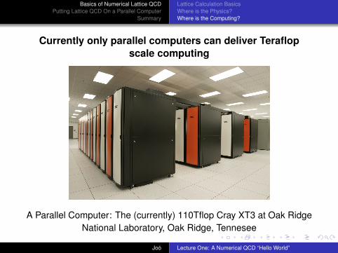
Currently only parallel computers can deliver Teraflopscale computing
A Parallel Computer: The (currently) 110Tflop Cray XT3 at Oak RidgeNational Laboratory, Oak Ridge, Tennesee
Joó Lecture One: A Numerical QCD “Hello World”

Basics of Numerical Lattice QCDPutting Lattice QCD On a Parallel Computer
Summary
Lattice Calculation BasicsWhere is the Physics?Where is the Computing?
Complete Big Picture
A credible lattice calculation is a formidable undertakingRequires:
Large amount (Teraflops) of computer time (Politics)Effective collaboration at the various levels (Management)Technical Know How at various levels (Physics, Algorithms,Code Development and Porting, Engineering, Analysis)Infrastructure: Hardware, Software, Grids, Tapes, etc
Tendencies:Large Collaborations (LHPC, MILC, UKQCD, ETMC etc)Multi-year planned data production runsInter Collaboration Collaborations are now appearing e.g:USQCD, USQCD-UKQCD collaborationsEmergence of “Infrastructure Groups”
provide software/hardware for you (eg: USQCD Nat. Fac.)provide services/data for you (eg: ILDG: LDG, DiGS, LDG,CSSM, JLDG)
Joó Lecture One: A Numerical QCD “Hello World”

Basics of Numerical Lattice QCDPutting Lattice QCD On a Parallel Computer
SummaryBasics of Parallel Computing
Basics of Parallel Computing
Tasks that don’t depend on each other can be donesimultaneouslyTypes of parallelism in problems:
Embarassing/Comfortable: Tasks completely independentCan make effective use of a collection of independent PCs
Closely coupled: tasks exchange information frequently(eg: share data)
Efficient information exchange needed: Shared memory /Networkeg: PC Cluster machines (with network), Supercomputers
Loosely coupled: tasks exchange information infrequentlySpeed of information exchange not critical, use internet etc.eg: managing a large collection of jobs on a Grid.
Lattice QCD is closely coupled
Joó Lecture One: A Numerical QCD “Hello World”

Basics of Numerical Lattice QCDPutting Lattice QCD On a Parallel Computer
SummaryBasics of Parallel Computing
Recent Trends in Hardware
Massively Parallel Systems (MPP): Contain O(10000)processing elements (PEs)Message Passing between PEs
Fast Custom Networks (BG/L, QCDOC, Cray XT3/4, APE)Commodity Networks on Clusters (eg infiniband)
Multi-Socket/Multi-Core PEsQCDOC and BG/L have 2 processors per node cardCray and Clusters employ multi-core chips (Intel, AMD)
Some amount of vectorization on PEsBG/L has “double hummer” FPU - 2 FPUs in oneCray and Clusters have SSE, SSE2, SSE3 instructions
Joó Lecture One: A Numerical QCD “Hello World”

Basics of Numerical Lattice QCDPutting Lattice QCD On a Parallel Computer
SummaryBasics of Parallel Computing
A Useful Model Computer
The processing elements form a gridEach processor can communicate with neighbours
Some machines are built like this (QCDOC, BG/L)Can be implemented “virtually” on machines with richerconnectivity or shared memory.
Joó Lecture One: A Numerical QCD “Hello World”

Basics of Numerical Lattice QCDPutting Lattice QCD On a Parallel Computer
SummaryBasics of Parallel Computing
Message Passing
For plaquette:Ux+µ̂ is put in message (proc 1 to 0)U†
x+ν̂ is put in message (proc 2 to 0)
Joó Lecture One: A Numerical QCD “Hello World”

Basics of Numerical Lattice QCDPutting Lattice QCD On a Parallel Computer
SummaryBasics of Parallel Computing
Collective Operations
Collective operations are called by all PEsThere are the following kinds:
Local collectives: each node gets own answerGathers: one (some) gets answer from manyScatters: many gets answer from one (some)
Broadcasts: one node sends to allAll to all: all get answers from all
Reductions: eg global sum, min, max
Joó Lecture One: A Numerical QCD “Hello World”

Basics of Numerical Lattice QCDPutting Lattice QCD On a Parallel Computer
SummaryBasics of Parallel Computing
The Message Passing Interface (MPI)The International Message Passing StandardRich Data ModelMany different ways to pass messagesQuite complexhttp://www-unix.mcs.anl.gov/mpi
The QCD Message Passing (QMP) InterfaceDesigned by USQCD SciDAC software committeeSimple data modelAsynchronous Sends OnlyRelatively easy to implement/use:
over MPIover custom networks (QCDOC, GigE mesh)http://usqcd.jlab.org/usqcd-docs/qmp
Joó Lecture One: A Numerical QCD “Hello World”

Basics of Numerical Lattice QCDPutting Lattice QCD On a Parallel Computer
SummaryBasics of Parallel Computing
Data Parallelism
Convenient programming modelEverything is collective“Shift Lattice” to get at neighbours“Global” fill operationsLimited by “masks”Try not to refer to an individual siteDoesn’t feel really parallel at all (Good!)Similar to CM-Fortran, HPF, F90
Joó Lecture One: A Numerical QCD “Hello World”

Basics of Numerical Lattice QCDPutting Lattice QCD On a Parallel Computer
SummaryBasics of Parallel Computing
How Shifts Work
Joó Lecture One: A Numerical QCD “Hello World”

Basics of Numerical Lattice QCDPutting Lattice QCD On a Parallel Computer
SummaryBasics of Parallel Computing
The SciDAC software stack for Lattice QCD
Joó Lecture One: A Numerical QCD “Hello World”

Basics of Numerical Lattice QCDPutting Lattice QCD On a Parallel Computer
Summary
Rest of tutorial
For the HPC sectionsWe will work with a data parallel frameworkWe will use a freely available library: QDP++
For the last lecture (Analysis)We will use some real and recent data
Sadly I don’t have time to cover ChromaBut most of the QDP++ examples are taken from chromaAfter the tutorial you should find chroma codestraightforward
Joó Lecture One: A Numerical QCD “Hello World”

Basics of Numerical Lattice QCDPutting Lattice QCD On a Parallel Computer
Summary
Summary Of Lecture
I discussed the gross details of a lattice calculationI discussed aspects of parallelismNow: Let’s write some code
Joó Lecture One: A Numerical QCD “Hello World”
Recommended