
Evgeny Hahamovich*, Sagi Monin*, Yoav Hazan and Amir Rosenthal 1 2 * Equal contribution 3
1. System setup 4
5 A detailed system setup is presented in Sup. Fig. 1. The light emitted by a 625 nm LED (Thorlabs, 6 M625L4) was focused on an area of the coded mask. The spatially coded light at the mask’s output 7 was collected by an infinity corrected objective lens (Nikon, N10X-PF). A small mismatch between the 8 stage’s center of rotation and center of the circular pattern led to a periodic movement of the coded 9 light in the radial direction, corresponding to a periodic change in the angle of the beam at the infinity 10 space of the objective lens. To compensate for the angular movement of the beam, a piezo-controlled 11 tip/tilt mirror (Physical Instruments, S-335) was used. The control signal to the mirror (Physical 12 Instruments, E727.x) was synchronized with the mask rotation rate and created a periodic change in 13 the mirror angle, compensating for the tilt of the beam. The beam was then directed to a tube lens, 14 which formed a ×10 magnified image of the projected pattern in the image plane. In the image plane, 15 an aperture was positioned in front of the imaged object to block light originating from mask regions 16 outside the relevant coded region. The light passing through the imaged object was collected via a 35 17 mm convex lens and focused on a single photodetector (Thorlabs, DET 36A-Si). The output signal from 18 the photodetector was amplified by a transimpedance amplifier and captured by a digital oscilloscope 19
A new spin on single-pixel imaging: spatial light modulation at megahertz switch rates
via cyclic Hadamard masks
Supplementary material
Supplementary Fig. 1 | Detailed system setup. L1 – Collimation lens, L2 – Tube lens, L3 – Focusing lens, Obj –
objective lens, A – aperture, PD – photodiode. Both the object and the aperture are placed in the imaging plane.
The lines between the different components indicates communication between them.
ilt p irror
ota on stage
isk
maging plane
cope ilt p mirror
controller
omputer ota on stage
controller

(Keysight, DSOX4154A). The mask was rotated at a frequency of up to 10 Hz by an air-bearing rotation 20 stage (Physical Instrument, A-625.025) controlled by a motion controller (Physical Instrument, 21 C891.130300). 22
23
2. Tiling geometry 24
Two types of tiling geometries were used in this work: hexagonal elements combined with circular 25 illumination beam shape (Sup. Fig. 2a) and square elements combined with rectangle illumination 26 beam shape (Sup. Fig. 2b). In both cases, the 1D cyclic codes were transformed into 2D patterns by 27 replicating the 1D code over all the rows of the 2D, where each row was cyclically shifted by several 28 elements with respect to the preceding row. Using this arrangement, a linear translation in the 2D 29 pattern corresponded to cyclic shifts in the 1D code, as illustrated in Sup. Fig. 2. In both tilling 30 geometries, the illumination coming from outside of the required pattern area was blocked by an 31 aperture. 32 33 In the following list, we specify the mask parameters used for each of the images and videos produced 34 in our work: 35 36 1. Fig. 3a, 3c, and 3d – Circular illumination beam divided to hexagon elements grid with a=3 µm, 37
corresponding to a horizontal distance of 5.2 µm and a vertical distance of 4.5 µm between the 38 elements. An objective lens on the optical channel magnified the pixels by 10 during the projection 39 to the image plane. Accordingly, the diameter of the imaged region was 8.7 mm. 40
2. Fig. 3b – Circular illumination beam divided to hexagon elements grid with a=0.85 µm, 41 corresponding to a horizontal distance of 1.47 um and vertical distance of 1.275 um between the 42 elements. An objective lens on the optical channel magnified the pixels by 10 during the projection 43 to the image plane. Accordingly, the diameter of the imaged region was 2.46 mm. 44
Supplementary Fig. 2 | Pattern geometry. a, from left to right: Pattern geometry for hexagon grid, an example
of S-matrix created with Quadratic Residue algorithm with N=7 elements, an illustration of the element
arrangement on the quartz plate, and the circular geometry of the illumination pattern that was coded to N
pixels. The different colors correspond to the different coded patterns (pattern 1, 2 and 5). b, from left to right:
Pattern geometry for square grid, an example of S-matrix created with twin-prime algorithm with N=15 (3x5)
element, an illustration of the elements arrangement on the quartz plate, and the rectangle geometry of image
size of N=PxQ pixels. The different colors correspond to the different coded patterns (pattern 1,2 and 5).

3. Fig. 3e – Rectangle illumination beam divided to square elements grid with a=4 µm. Two combined 45 objective lenses (x10 and an inverted x20) on the optical channel decreased the size of the pixels 46 by 2 during the projection to the image plane. Accordingly, the diameter of the imaged region was 47 0.2 mm. 48
4. Fig. 4a and the corresponding video recordings – Rectangle illumination beam divided to square 49 elements grid with a=4 µm. An objective lens on the optical channel magnified the pixels by 10 50 during the projection onto the image plane. Accordingly, the diameter of the imaged region was 51 4 mm. 52
5. Fig. 4b and 4c and the corresponding video recordings – Circular illumination beam divided to 53 hexagon elements grid with a=3 µm, corresponding to a horizontal distance of 5.2 µm and a 54 vertical distance of 4.5 µm between elements. Two combined objective lenses (x10 and an 55 inverted x20) on the optical channel decreased the size of the pixels by 2 during the projection 56 onto the image plane. Accordingly, the diameter of the imaged region was 0.44 mm. 57
58 In our analysis, we assumed that all elements in each 2D pattern were of the same size. However, 59 since the patterns were fabricated over a circular path, small differences were obtained between inner 60 and outer diameters of the pattern, leading to minor variations in the element size over the pattern’s 61 width. However, as we show in the following, the small difference between the inner and outer 62 diameters of the geometrical ring over which pattern was fabricated led to negligible variation in the 63 elements’ width. For example, for the images presented in Fig. 4a in the paper, the aperture size was 64 404 𝜇𝑚 × 412 𝜇𝑚, and the pattern was located 57.2 𝑚𝑚 away from the center of rotation, depicted 65 in Sup. Fig. 3. Therefore, the difference between the inner and the outer element size was 66 approximately 0.03 𝜇𝑚, corresponding to a mere 0.75% maximum change in element size. 67 Furthermore, since the critical-dimension uniformity of the photomask was also approximately 68 0.03 𝜇𝑚, the geometrical variation in element size falls within the manufacturing-error range. 69 70 Supporting calculation: 71
Angle: 𝜃 = arctan (412
57200) = 0.0072 72
Total width for external radius: 57402 ⋅ tan(0.0072) = 413.89 𝜇𝑚 73
Total width for internal radius: 56998 ⋅ tan(0.0072) = 410.4 𝜇𝑚 74
Total difference is 3.4 𝜇𝑚, and element difference is 3.4
103= 0.03 𝜇𝑚 75
76
Supplementary Fig. 3 | Pattern variation due to the circular geometry of pattern aperture. Example for Fig.4a
of the paper, with pattern distance of 57.2𝑚𝑚 and element size of 4𝜇𝑚 results in difference of 30𝑛𝑚 for
element size.

3. Calibration 77
Since the center of rotation and the center of 78 the fabricated patterns did not perfectly 79 coincide, rotation led to a harmonic movement 80 of the patterns in the radial direction, which 81 translated to a lateral movement of the 82 illumination pattern on the imaged object. To 83 compensate for this eccentricity and minimize 84 the lateral movement of the illumination 85 pattern, a tip/tilt mirror, positioned in the 86 infinity space of the objective lens (Sup. Fig. 1) 87 was scanned to create a counter lateral 88 movement in the image plane, using the 89 following protocol: 90 91 92 1. Radial-shift measurement: The imaged 93
object was replaced by a camera (Thorlabs, 94 DCC1545). A calibration pattern of 95 circumference was drawn on the quartz 96 mask and was projected on the camera. 97 The disk was rotated through all the 98 measured angles and the offset of the 99 projected circumference was measured 100 per angle. The results of this eccentricity 101 measurement are presented in Sup. Fig 4. 102 103
2. Calibration: Based on the recorded offset, an arbitrary waveform was programed to the tilt/tip 104 mirror controller (Physical Instrument, E727.x). 105 106
3. Real-time compensation: During the measurements, the mirror was continuously moved based 107 on the injected waveform, compensating for the eccentricity of the system. 108
109 An additional effect of the radial movement of the quartz masks is a modulation of the tangential 110 velocity of the projected pattern. Specifically, since the tangential velocity is a product of the 111 approximately constant rotation velocity and the pattern’s radius, the harmonic pertur ation in the 112 radius is linearly translated into harmonic variation in the tangential velocity and in the rate in which 113 the base functions are switched. To compensate for this effect, the measured offset was used to 114 update the sampling grid during the reconstruction process of the image. 115 116
Supplementary Fig. 4 | Eccentricity measurement of
quartz plate. Measured eccentricity of the of the system.
The plate was rotated through all angles in the range of
0-360 degrees.

4. Velocity Tracking Method 117
118 Although no drift in the rotation speed was observed 119 in our experiments, it is desirable for our scheme to 120 be robust against such drifts to make it compatible 121 with less accurate stages. To compensate for potential 122 velocity drifts, the tangential velocity should be 123 monitored in real time. In this section we describe a 124 method for velocity monitoring that can be integrated 125 in our imaging setup. 126 127 To enable real-time monitoring of the rotation speed, 128 we fabricated a periodic pattern on the photomask, 129 composed of segmented lines with 50% duty-cycle 130 presented (Sup. Fig. 5). A light source was focused 131 onto the pattern with a spot size significantly smaller 132 than the pattern’s width. he light transmitted 133 through the segmented lines was measured by a 134 photodiode, leading to a signal that alternated 135 between the two states. Denoting the length of one full cycle by x, and the alternation time between 136 two consecutive cycles with 𝑡𝑖, the velocity was calculated using 𝑣𝑖 = 𝑥/𝑡𝑖. 137 138 This configuration was experimentally examined by measuring the rotation speed of an accelerating 139 stage. Measurement results are shown in Sup. Fig. 6, showing the signal captured by the photodiode 140 (6.a and 6.b.) and the extracted velocity (6.c). 141 142 The technique described above may be used to monitor the rotation speed of the photomask during 143 the imaging session by adding a second photodetector to capture the transmission pattern from the 144
Supplementary Fig. 5 | Segmented lines
fabricated on circumference of the mask. The
image was captured with camera.
Supplementary Fig. 6 | Velocity measurement using the segmented line pattern. (a) voltage from the
photodetector recorded during stage acceleration, (b) zoom on the captured pattern and (c) the recovered
velocity of the stage as a function of time.

periodic pattern. Then, random drifts in velocity may be corrected in the post processing of the data, 145 using the same procedure applied for the deterministic velocity changes in Section 4 of the 146 Supplementary Information. 147
148 149
5. Image reconstruction and sampling matrix procedure 150
151 In our work we used 𝑺-matrix codes as the sampling matrix. The 𝑺-matrix is a well-known code based 152 on Hadamard codes1. In contrast to Hadamard codes, which are based on binary code of ±1′, 𝑺-matrix 153 codes are based on 0′s and 1′s. 𝑺-matrices have Paley construction, where the sampling matrix is 154 cyclic construction, where each row of the matrix is cyclic left shift of the previous row. 155 156
The reconstruction can be generally performed via a matrix multiplication of ˆ-1
x = S y , where x̂ is a 157
row stack vector representation of the recovered image, -1S is the inverse of the projection matrix and158
y is the measurement vector. The S-matrix has a closed-form solution for inverse matrix calculation 159
2(2 )
1
T
N= −
+
-1S S J , where J is a matrix of ’s and 𝑁 is the size of the matrix. However, performing 160
the reconstruction with a matrix-vector multiplication leads to computational complexity of 𝑂(𝑁2) 161 and memory requirements of of 𝑂(𝑁2), which may limit the implementation for large images. For 162 example, in our work the matrix occupied ~5 Gb of memory for 𝑁 = 25,111 when double-class 163 precision. 164 165 To accelerate the reconstruction, we propose an alternative algorithm that is based on Fast Fourier 166 Transform (FFT). Using the property of cyclic sampling, the sampling equation 𝒚 = 𝑺𝒙, can be 167 expressed as 𝒚 = 𝒔𝟏 ⊛ 𝒙 , where 𝒔𝟏 is the first row of the sampling matrix, and ⊛ is the circular 168 convolution operator. By circular convolution theorem2 we can express the sampling equation with 169 FFT: 𝐹{𝒚} = 𝐹{𝑺𝟏} ⋅ 𝐹{𝒙}, where 𝐹{} denotes the FFT operator, and the image can be reconstructed 170 by �̂� = 𝐹−1{𝐹{𝒚}/𝐹{𝑺𝟏}}. Reconstruction with FFT is of computational complexity of 𝑂(𝑁𝑙𝑜𝑔𝑁) 171 and memory requirements of 𝑂(𝑁), accelerating reconstruction time greatly and reducing memory 172 requirements, thus facilitating the reconstruction of large images. In this work, the reconstruction of 173 images with 𝑁 = 25,111 was performed in 4 ms on a CPU without any parallel computations and 174 required a memory of 0.4 Mb with complex double-class precision for storing 𝐹{𝑺𝟏}. 175 176
177
178
179
180
181
182
183
184
185
186
187
188
189

6. Gray level image comparison to a reference camera image 190
191
To demonstrate the capability of our scheme for imaging gray-scale images, we tested it on an old 192 photographic film containing an image of flowers. The resulting SPI reconstruction, presented in Fig. 193 3d of the main paper, is compared in this section to an image of the film taken with a scientific camera 194 (Thorlabs, DCC1545). For a fair comparison between the images, we resized the camera image, from 195 the original 1280 x 1024 pixels, to the resolution of the SPI image. The comparison presented in Sup. 196 Fig. 7, shows a very good visual agreement between the two images. 197 198
199
200 201
202
203
204
205
206
207
208
209
210
211
212
213
214
215
Supplementary Fig. 7 | Gray level image of a flowers slide. An image of an old photographic slide with gray
levels captured with our SPI system (left) is compared to a reference image (right) taken with a camera.

7. The effect of averaging sub-pixel-shifted images 216
217
In this section, we demonstrate the benefit of using sub-pixel shifts in the image reconstruction, as 218
discussed in Fig. 2 of the main paper. During the measurement, the analog signal is sampled at a high 219
sample rate, with a temporal resolution significantly above the switching time between two 220
neighboring patterns, 𝑇. For an over-sampling factor of 𝑀, we obtain 𝑀 distinct reconstructions, which 221
are shifted with respect to one another by Δ/𝑀, where Δ is the pixel width; all 𝑀 images are realigned 222
and averaged to obtain the final reconstruction. 223
As demonstrated in the following examples, averaging the images after sub-pixel realignment can 224
produce images with higher contrast in comparison to direct approach in which realignment is not 225
used and better SNR in comparison to a single sub-pixel reconstruction. In the first example, we 226
consider an alternative reconstruction strategy in which the images are averaged without 227
realignment. Sup. Fig. 8 shows the resulting reconstructions of the resolution target shown in Fig. 3.a 228
with (Sup. Fig. 8a) and without (Sub. Fig. 8b) realignment and compares 1D slices taken over various 229
positions on the targets (Sup. Fig. 8c-8f). As can be seen in the reconstructions of Targets 3.1 and 3.2, 230
realigning the images enhances the contrast of fine details in the image. 231
In the second example, we tested the SNR gain achieved by averaging the 𝑀 images over using only a 232
single image on the example of Fig. 3.b, which was captured with the maximum imaging rate of our 233
system, 2.4 megapixel/sec. Generally, for sufficiently high imaging rates the main noise source in the 234
reconstructions is noise in the photodetector output, whose magnitude is proportional to the square 235
root of the imaging duration. Under this noise model, reconstructions performed by averaging 𝑀 236
Supplementary Fig. 8 | Comparison of image reconstruction from over-sampled data with and without image
realignment. 𝑀 =5 slightly shifted experimental reconstructions of a resolution target were produced and
summed to produce the final reconstruction (a) with and (b) without performing sub-pixel realignment before
summation. (c)-(f) a comparison between the 1D slices of resolution targets 2.5, 2.6, 3.1 and 3.2, reconstruction
with (red) and without (blue) realignment.
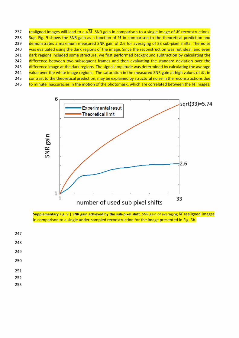
realigned images will lead to a √𝑀 SNR gain in comparison to a single image of 𝑀 reconstructions. 237
Sup. Fig. 9 shows the SNR gain as a function of 𝑀 in comparison to the theoretical prediction and 238
demonstrates a maximum measured SNR gain of 2.6 for averaging of 33 sub-pixel shifts. The noise 239
was evaluated using the dark regions of the image. Since the reconstruction was not ideal, and even 240
dark regions included some structure, we first performed background subtraction by calculating the 241
difference between two subsequent frames and then evaluating the standard deviation over the 242
difference image at the dark regions. The signal amplitude was determined by calculating the average 243
value over the white image regions. The saturation in the measured SNR gain at high values of 𝑀, in 244
contrast to the theoretical prediction, may be explained by structural noise in the reconstructions due 245
to minute inaccuracies in the motion of the photomask, which are correlated between the 𝑀 images. 246
247
248
249
250
251
252
253
Supplementary Fig. 9 | SNR gain achieved by the sub-pixel shift. SNR gain of averaging 𝑀 realigned images
in comparison to a single under-sampled reconstruction for the image presented in Fig. 3b.

8. Sampling matrix formation procedure 254
255
The S-matrix codes were generated by the Quadratic Residue algorithm for the hexagon patterns (Sup. 256
Fig. 2.a) and by the Twin Prime algorithm for square patterns (Sup. Fig. 2.b)1. Detailed construction 257
algorithms are: 258
Algorithm 1: Quadratic Residue Construction of S-matrix Input : n - number of elements in matrix. The number must be a prime number of the form 4 3m+ ,
where m is an integer
Step 1 : Create vector:
2[1,4,9,..., (( 1) / 2) ]a n= −
Step 2 : Calculate remainder of a by n , ( , )b rem a n=
Step 3 : Create a vector of zeros (1: ) 0s n = .
Step 4 : Add +1 to vector s in b indexes, [ ] 1s b =
Step 5 : For 0 : 1i n= −
Cyclic shift vector s to the left by i , ( , )s shift s i=
Insert vector to
thi row of matrix, [ ,:]i sS
end
s
Algorithm 2: Twin-prime Construction of S-matrix Input : p - where p and 2q p= + are both prime number and n p q= - number of elements in
matrix Step 1 : Create vector: 0 : 1a n= −
Step 2 : Calculate remainder of a by p , ( , )fb rem a p=
Step 3 : Create vector:
2[1, 4,9,..., (( 1) / 2) ]fc p= −
Step 4 : Calculate remainder of fc by p , ( , )f fd rem c p=
Step 5 : Create a vector of -1, (1: ) 1f n = − .
Step 6 : Add +1 to vector f in fb indexes, [ ] 0fs b =
Step 7 : For 0 : 1i q= −
Add +2 to vector f in fd i p+ indexes, [ ] 1fs d i p+ =
End Step 8 :
Calculate remainder of a by q , ( , )gb rem a q=
Step 9 : Create vector:
2[1, 4,9,..., (( 1) / 2) ]gc q= −
Step 10 : Calculate remainder of gc by q , ( , )g gd rem c p=
Step 11 : Create a vector of -1, (1: ) 1g n = − .
Step 12 : Add +1 to vector g in gb indexes, [ ] 0gs b =
Step 13 : For 0 : 1i p= −
Add +2 to vector g in gd i p+ indexes, [ ] 1gs d i p+ =
End Step 14 : Create a vector of ones (1: ) 1s n = .
Step 15 : Set 0 to vector s in indexes where f g== , [ ] 0s f g== =
Step 16 : Set 0 to vector s in indexes [0, , 2 ,..., ( 1) ]q q p q− , [0, , 2 ,..., ( 1) ] 0s q q p q− =
Step 17 : For 0 : 1i n= −
Cyclic shift vector s to the left by i , ( , )s shift s i=
Insert vector to
thi row of matrix, [ ,:]i sS
End

9. Compressed sensing 259
260 261 262
263
While the results presented in the paper use full base acquisition and reconstruction, it is possible to 264
reduce the required number of measurements by algorithmic reconstruction optimization via 265
compressed sensing. We demonstrate this by performing image reconstruction from under sampled 266
datasets with 75%, 50%, 33% and 25% of the samples. We show a comparison of three under-sampling 267
methods: 268
1) Signal truncation: The signal is truncated, leading to a reduced dataset in which samples are 269
consecutive. 270
2) Uniform under-sampling: We take every 𝑛𝑡ℎ sample of the original dataset, where 𝑛 = 2,3,4, 271
to form the reduced dataset. For example, for 75% we omit every 4th measurement. 272
3) Random under-sampling: The samples of the reduced dataset are randomly chosen from the 273
full dataset. 274
Supplementary Fig. 10 | Compressed sensing image restoration based on partial data. The Technion logo
image is recovered from partial samples with different sampling procedures.
Supplementary Table 1 | SSIM comparison of the CS
reconstructions. Comparison was conducted between
CS results and a full base reconstruction with 100% of
the measurements.
Supplementary Table 2 | PSNR comparison of the CS
reconstructions. Comparison was conducted between
CS results and a full base reconstruction with 100% of
the measurements.
For all cases, the reconstruction was performed by a TVAL3 algorithm3, solving a compressed sensing 275
problem with total variation regularization. This algorithm was proposed for single-pixel imaging4 and 276
demonstrated in different SPI scenarios5–7. Identical hyper-parameters were used for all the compared 277
reconstructions. 278
The reconstruction results are presented in Sup. Fig. 10 for the Technion logo. To quantify the 279
reconstruction quality, the SSIM and PSNR values were calculated between the CS reconstructions and 280
the full-data reconstruction, using the following equations: 281
For two images, 𝐼 and 𝐽, structural similarity (SSIM) is calculated by the following equation: 282
𝑆𝑆𝐼𝑀 =(2𝜇𝐼𝜇𝐽 + 𝑐1)(2𝜎𝐼𝐽 + 𝑐2)
(𝜇𝐼2 + 𝜇𝐽
2 + 𝑐1)(𝜎𝐼2 + 𝜎𝐽
2 + 𝑐2), 283
where 𝜇𝐼 and 𝜇𝐽 are averages of the two compared images, 𝜎𝐼2 and 𝜎𝐽
2 are the variances of the images, 284
𝜎𝐼𝐽 is the covariance, and 𝑐1 and 𝑐2 are two variables calculated from the dynamic range of the images. 285
For two images, 𝐼 and 𝐽 of sizes [𝑋, 𝑌], peak signal-to-noise ratio (PSNR) is calculated by the following 286
equation: 287
𝑃𝑆𝑁𝑅 = 10 log10 (𝑀𝐴𝑋𝐼
2
𝑀𝑆𝐸) = 10 log10 (
𝑀𝐴𝑋𝐼2
1𝑋𝑌
∑ ∑ |𝐼(𝑥, 𝑦) − 𝐽(𝑥, 𝑦)|2𝑌−1𝑦=0
𝑋−1𝑥=0
), 288
where 𝑀𝐴𝑋𝐼 is the maximum values over the image 𝐼. 289
The SSIM and PSNR values are summarized in Sup. Tables 1 and 2. The figure and tables clearly show 290
that uniform and random under-sampling led to better reconstructions than signal truncation. 291
Nonetheless, even in the case of signal truncation, the Technion logo was clearly visible with 50% of 292
the measurement data. Accordingly, it should be possible to increase the imaging rate by 2 while 293
acquiring only half of the base and reconstructing the image with the described compressive sampling 294
algorithms, achieving imaging rate of up to 4.8 mega pixels per second. 295
296
297
298

10. Video recording 299
300 Three videos captured by our system are attached as Supplementary Videos 1-3. Several frames from 301
each video are presented in Fig. 4 of the main paper. Each frame followed the same reconstruction 302
procedure as the individual images, as described in Supplementary section 5. 303
Detailed configuration per video recording are listed below: 304 305 1. Resolution target motion (Fig.4.a, Sup . Vid. 1): Total of 142 consecutive frames, captured at a 306
frame rate of 72 fps with 10,403 pixels per frame. The video captures a vertical scan of a standard 307 resolution target. A rectangle illumination beam divided to square elements grid (Sup. Fig. 2.b.) 308 was used, with x10 optical magnification of the object, leading to a pixel size of 40 um (4 um x 10). 309 310
2. Worm motion (Fig. 4b and 4c, Sup. Vid.2 and 3): Total of 31 consecutive frames captured at a 311 frame rate of 10 fps with 25,111 pixels per frame. The videos captured the in vivo motion of C. 312 elegans worms. A circular illumination beam divided to hexagon elements grid (Sup. Fig. 2a) was 313 used, with x0.5 magnification of the object, leading to a pixel size of 2.6 µm. 314
315 316
317
11. References 318
319 1. Harwit, M. Hadamard transform optics. (Elsevier, 1979). doi:10.1016/B978-0-12-330050-320
8.50001-9 321 2. Yin, W., Morgan, S., Yang, J. & Zhang, Y. Practical compressive sensing with Toeplitz and 322
circulant matrices. Vis. Commun. Image Process. 2010 7744, 77440K (2010). 323 3. Li, C., Yin, W., Jiang, H. & Zhang, Y. An efficient augmented Lagrangian method with applications 324
to total variation minimization. Comput. Optim. Appl. 56, 507–530 (2013). 325 4. Li, C. An Efficient Algorithm For Total Variation Regularization with Applications to the Single 326
Pixel Camera and Compressive Sensing. (2009). 327 5. Howland, G. A., Lum, D. J., Ware, M. R. & Howell, J. C. Photon counting compressive depth 328
mapping. Opt. Express 21, 23822 (2013). 329 6. Yang, J. & Zhang, Y. lternating direction algorithms for ℓ -problems in compressive sensing. 330
SIAM J. Sci. Comput. 33, 250–278 (2011). 331 7. Howland, G. A., Lum, D. J. & Howell, J. C. Compressive wavefront sensing with weak values. 332
Opt. Express 22, 18870 (2014). 333 334
335
Recommended


![Video coding [??]. Video coding Types of redundancies: – Spatial: Correlation between neighboring pixel values – Spectral: Correlation between different](https://img.dokumen.tips/doc/110x75/56649e635503460f94b5fcc5/video-coding-video-coding-types-of-redundancies-spatial-correlation.jpg)


![CS-MUVI: Video Compressive Sensing for Spatial ...vip.ece.cornell.edu/papers/12ICCP-csmuvi.pdf · applications. Spatial-multiplexing cameras: The single-pixel camera (SPC) [3], the](https://img.dokumen.tips/doc/110x75/5f747cf77ea9f1395139a8cb/cs-muvi-video-compressive-sensing-for-spatial-vipece-applications-spatial-multiplexing.jpg)