WORK ING PAPER S ER I E SNO. 405 / NOVEMBER 2004
A JOINT ECONOMETRIC MODEL OF MACROECONOMIC
DYNAMICS
by Peter Hördahl, Oreste Tristaniand David Vestin
AND TERM STRUCTURE

In 2004 all publications
will carry a motif taken
from the €100 banknote.
WORK ING PAPER S ER I E SNO. 405 / NOVEMBER 2004
A JOINT ECONOMETRIC
MODEL OF MACROECONOMIC
DYNAMICS 1
by Peter Hördahl 2, Oreste Tristani 3
and David Vestin 4
1 The opinions expressed in this paper are those of the authors and do not necessarily reflect the views of the European Central Bank.2 DG Research, European Central Bank; e-mail: [email protected]
3 Corresponding author: DG Research, European Central Bank, Kaiserstrasse 29,D-60311 Frankfurt am Main, Germany; e-mail: [email protected],
tel.: +49 69 1344 7373, fax: +49 69 1344 8553.4 DG Research, European Central Bank; e-mail: [email protected]
This paper can be downloaded without charge from http://www.ecb.int or from the Social Science Research Network
electronic library at http://ssrn.com/abstract_id=601025.
AND TERM STRUCTURE

© European Central Bank, 2004
AddressKaiserstrasse 2960311 Frankfurt am Main, Germany
Postal addressPostfach 16 03 1960066 Frankfurt am Main, Germany
Telephone+49 69 1344 0
Internethttp://www.ecb.int
Fax+49 69 1344 6000
Telex411 144 ecb d
All rights reserved.
Reproduction for educational and non-commercial purposes is permitted providedthat the source is acknowledged.
The views expressed in this paper do notnecessarily reflect those of the EuropeanCentral Bank.
The statement of purpose for the ECBWorking Paper Series is available from theECB website, http://www.ecb.int.
ISSN 1561-0810 (print)ISSN 1725-2806 (online)

3ECB
Working Paper Series No. 405November 2004
CONTENT S
Abstract 4
Non-technical summary 5
1 Introduction 7
2 The approach 8
2.1 A simple backward/forwardlooking macroeconomic model 10
2.2 A general macroeconomic set-up 13
2.3 Adding the term structure to the model 14
2.4 Maximum likelihood estimation 17
3 An application to German data 19
3.1 Data 19
3.2 Estimation results 19
3.2.1 Parameter estimates 20
3.2.2 Impulse response functions 23
3.3 Macro shocks and risk premia 24
4 Forecasting 26
4.1 Do yields help to forecastmacroeconomic variables? 27
4.2 Do macroeconomic variables help toforecast yields? 28
5 Expectations hypothesis tests 31
5.1 LPY(i) 33
5.2 LPY(ii) 34
6 Conclusions 35
Appendix 38
References 46
Tables and figures 50
European Central Bank working paper series 65

Abstract
We construct and estimate a joint model of macroeconomic and yield curvedynamics. A small-scale rational expectations model describes the macroecon-omy. Bond yields are affine functions of the state variables of the macromodel,and are derived assuming absence of arbitrage opportunities and a flexible priceof risk specification. While maintaining the tractability of the affine set-up, ourapproach provides a way to interpret yield dynamics in terms of macroeconomicfundamentals; time-varying risk premia, in particular, are associated with thefundamental sources of risk in the economy. In an application to German data,the model is able to capture the salient features of the term structure of interestrates and its forecasting performance is often superior to that of the best avail-able models based on latent factors. The model has also considerable success inaccounting for features of the data that represent a puzzle for the expectationshypothesis.
JEL classification: E43, E44, E47Keywords: Affine term-structure models, policy rules, new neo-classical
synthesis
4ECBWorking Paper Series No. 405November 2004

Non-technical summary
This paper aims at deepening our understanding of how macroeconomic fac-
tors drive movements in the term structure of interest rates and how they affect the
behavior of risk premia embedded in observed yields. While this has long been a
topic on the agenda of both financial and macro economists, the focus of research
as well as the methods used have often been different. On the one hand, financial
economists have mainly focused on forecasting and pricing interest rate related se-
curities. They have therefore developed powerful models based on the assumption
of absence of arbitrage opportunities, but typically left unspecified the relationship
between the term structure and other economic variables. Macro economists, on the
other hand, have focused on understanding the relationship between interest rates,
monetary policy and macroeconomic fundamentals. In so doing, however, they have
typically not imposed restrictions to preclude arbitrage opportunities and they have
often ignored the role of time-varying risk premia as an important component in
explaining movements in yields over time. In other words, macro economists have
typically relied on the “expectations hypothesis” (i.e. assumed zero or constant risk
premia) in spite of its poor empirical record.
This paper combines the two lines of research and presents a unified empiri-
cal framework where a small structural model of the macro economy is combined
with an arbitrage-free model of bond yields. The proposed model extends the term
structure literature, since it shows how to derive bond prices using no-arbitrage
conditions based on an explicit structural macroeconomic model, including both
forward-looking and backward-looking elements. At the same time, we extend the
macroeconomic literature by studying the term structure implications of a standard
macro model within a dynamic no-arbitrage framework. The fact that we use a
structural macroeconomic framework, rather than a reduced-form VAR representa-
tion of the data, is one of the main innovative features of our paper. One of the
advantages of this approach is that it facilitates an economic interpretation of the
results.
5ECB
Working Paper Series No. 405November 2004

In an empirical application using German data, we show that there are syn-
ergies to be exploited from modelling the term structure of interest rates using a
combination of macro and finance approaches, and that this gives rise to sensible
results. Notably, we show that our estimates of macroeconomic parameters, that are
partly determined by the term-structure data, are consistent with those that would
be estimated using only macroeconomic information. At the same time, our model’s
explanatory power for the term-structure is comparable to that of state-of-the-art
term-structure models based only on unobservable variables.
We find that our model performs very well in terms of two evaluation criteria
that we employ, namely the model’s out-of-sample yield forecasting performance and
the ability of the model to account for deviations from the expectations hypothesis
in the observed term structure. We argue that the model’s success is due to both the
inclusion of macroeconomic variables in the information set and to the imposition of
a large number of no-arbitrage and structural restrictions. The fact that we are able
to account for deviations from the expectations hypothesis demonstrates that the
dynamics of stochastic risk premia are important determinants of yield dynamics.
Since risk premia in our model are driven by macroeconomic fundamentals, we con-
clude that the dynamics of such premia can ultimately be attributed to underlying
macroeconomic dynamics within a consistent framework.
6ECBWorking Paper Series No. 405November 2004

1 Introduction
Understanding the term structure of interest rates has long been a topic on the
agenda of both financial and macro economists, albeit for different reasons. On the
one hand, financial economists have mainly focused on forecasting and pricing inter-
est rate related securities. They have therefore developed powerful models based on
the assumption of absence of arbitrage opportunities, but typically left unspecified
the relationship between the term structure and other economic variables. Macro
economists, on the other hand, have focused on understanding the relationship be-
tween interest rates, monetary policy and macroeconomic fundamentals. In so doing,
however, they have typically relied on the “expectations hypothesis,” in spite of its
poor empirical record. Combining these two lines of research seems fruitful, in that
there are potential gains going both ways.
This paper aims at presenting a unified empirical framework where a small
structural model of the macro economy is combined with an arbitrage-free model
of bond yields. We build on the work of Piazzesi (2003) and Ang and Piazzesi
(2003), who introduce macroeconomic variables into the standard affine term struc-
ture framework based on latent factors — e.g. Duffie and Kan (1996) and Dai and
Singleton (2000). The main innovative feature of our paper is that we use a structural
macroeconomic framework rather than starting from a reduced-form VAR represen-
tation of the data. One of the advantages of this approach is to allow us to relax
Ang and Piazzesi’s restriction that inflation and output be independent of the policy
interest rate, thus facilitating an economic interpretation of the results. Our frame-
work is similar in spirit to that in Wu (2002), who prices bonds within a calibrated
rational expectations macro-model. The difference is that we estimate our model
and allow a more empirically oriented specification of both the macro economy and
the market price of risk.1
Our estimation results, based on German data, show that macroeconomic fac-
1A framework similar to ours is also employed in recent papers by Rudebusch and Wu (2003),who interpret latent term structure factors in terms of macroeconomic variables, and by Bekaert,Cho and Moreno (2003), who mix a structural macro framework with unobservable term structurefactors.
7ECB
Working Paper Series No. 405November 2004

tors affect the term-structure of interest rates in different ways. Monetary policy
shocks have a marked impact on yields at short maturities, and a small effect at
longer maturities. Inflation and output shocks mostly affect the curvature of the
yield curve at medium-term maturities. Changes in the perceived inflation target
have more lasting effects and tend to have a stronger impact on longer term yields.
Our results also suggest that including macroeconomic variables in the infor-
mation set helps to forecast yields. The out-of-sample forecasting performance of
our model is superior to that of the best available affine term structure models for
most maturities/horizons.
Finally, we show that the risk premia generated by our model are sensible. First,
the model can account for the features of the data which represent a puzzle for the
expectations hypothesis, namely the finding of a negative and large — rather than
positive and unit — coefficients obtained, for example by Campbell and Shiller (1991),
in regressions of the yield change on the slope of the curve. Second, regressions based
on risk-adjusted yields do, by and large, recover slope coefficients close to unity, i.e.
the value consistent with the rational expectations hypothesis.
The rest of the paper is organized as follows. Section 2 describes the main
features of our general theoretical approach and then provides a brief overview of
our estimation method. It also discusses the specific macroeconomic model which we
employ in our empirical application. The estimation results, based on our application
to German data is described in Section 3. Section 4 then discusses the forecasting
performance of our model, compared to leading available alternatives. The ability of
the model to solve the expectations puzzle is tested in Section 5. Section 6 concludes.
2 The approach
In recent years, the finance literature on the term structure of interest rates has made
tremendous progress in a number of directions (see e.g. Dai and Singleton, 2003).
Following the seminal paper by Duffie and Kan (1996), one of the most successful
avenues of research has focused on models where the yields are affine functions of a
vector of state variables. This literature, however, has typically not investigated the
8ECBWorking Paper Series No. 405November 2004

connections between term structure and macroeconomic dynamics. In the rare cases
in which macroeconomic variables—notably, the inflation rate—have been included in
estimated term-structure models, those variables have been modelled exogenously
(e.g. Evans, 2003; Zaffaroni, 2001; Ang and Bekaert, 2004). The interactions be-
tween macroeconomic and term structure dynamics have also been left unexplored
in the macroeconomic literature, in spite of the fact that simple “policy rules” have
often scored well in describing the dynamics of the short-term interest rate (e.g.,
Clarida, Galí and Gertler, 2000).
An attempt to bridge this gap within an estimated, arbitrage-free framework
has recently been made by Ang and Piazzesi (2003).2 Those authors estimate a term
structure model based on the assumption that the short term rate is affected partly
by macroeconomic variables, as in the literature on simple monetary policy rules,
and partly by unobservable factors, as in the affine term-structure literature. Ang
and Piazzesi’s results suggest that macroeconomic variables have an important ex-
planatory role for yields and that the inclusion of such variables in a term structure
model can improve its one-step ahead forecasting performance. Nevertheless, unob-
servable factors without a clear economic interpretation still play an important role
in their model. Moreover, Ang and Piazzesi’s two-stage estimation method relies
on the assumption that the short term interest rate does not affect macroeconomic
variables.
In order to redress these shortcomings, we construct a dynamic term structure
model entirely based on macroeconomic factors, which allows for an explicit feedback
from the short term (policy) rate to macroeconomic outcomes. The joint modelling
of three key macroeconomic variables—namely, inflation, the output gap and the short
term “policy” interest rate—should allow us to obtain a more accurate (endogenous)
description of the dynamics of the short term rate. At the same time, our explicit
modelling or risk premia should also help us in capturing the dynamics of the entire
term-structure.
In this section, we present our approach to model jointly the macroeconomy
2In related papers, Dewachter and Lyrio (2002) and Dewachter, Lyrio and Maes (2002) alsoestimate jointly a term structure model built on a continuous time VAR.
9ECB
Working Paper Series No. 405November 2004

and the term structure. The main assumption we impose is that aggregate macro-
economic relationships can be described using a linear framework. To motivate our
approach, we start with an outline of the macroeconomic model that we use in our
empirical analysis. We then cast this macro-model in a more general framework
and show how to price bonds within such a framework based on the assumption of
absence of arbitrage opportunities.
2.1 A simple backward/forward looking macroeconomic model
We rely on a structural macroeconomic model, whose choice is motivated by the fact
that it could be derived from first principles. The model is certainly too stylized
— for example in its ignoring foreign variables or the exchange rate — to provide
a fully-satisfactory account of German macroeconomic dynamics. Nevertheless, it
does include the minimal structure of a macroeconomic model proper. Our results
in sections in Sections 4 and 5 suggest that such minimal structure does capture the
central features of the dynamics of yields.
The model of the economy includes just two equations which describe the evo-
lution of inflation, ��, and the output gap, ��:
�� = ���� [��+1] + (1− ��)��−1 + ���� + ��� �
�� = ������+1 + (1− ��)��−1 − �� (� −�� [��+1]) + ���
The inflation equation implies that prices will be set as a markup on marginal
cost, captured by the output gap term in the equation. The assumption of price
stickiness generates the expected inflation term, while the lags capture inflation in-
ertia. The output gap equation provides a description of the dynamics of aggregate
demand, which is assumed to be affected by movements in the short term real inter-
est rate. The forward looking term captures the intertemporal smoothing motives
characterizing consumption, the main component of aggregate demand.3
3Both equations can be derived from first principles. More precisely, the inflation equation can bederived as the first order condition of the price-setting decision of firms acting in an environment withmonopolistic competition. Monopolistic competition implies that prices will be set as a markup onmarginal cost, which explains the presence of the output gap term in the equation. The assumption
10ECBWorking Paper Series No. 405November 2004

The two equation above are often interpreted as appropriate to describe yearly
data. Since we will employ monthly data in estimation, we recast the model at the
monthly frequency using an approach similar to Rudebusch (2002). The equations
that we will actually estimate are therefore
�� =��
12
12X�=1
�� [��+�] + (1− ��)3X
�=1
�����−� + ���� + ��� � (1)
�� =��
12
12X�=1
�� [��+�] + (1− ��)3X
�=1
�����−� − �� (� −�� [��+11]) + ��� � (2)
where all variables now are expressed at the monthly frequency, and where inflation
is defined as �� ≡ ln��−ln��−12� where �� is the price level at �.4 The two equations
include a forward-looking term capturing expectations over the next twelve months
of inflation and output, respectively. The backward-looking components of the two
equations are restricted to include only 3 lags of the dependent variable. This
choice results in a more parsimonious empirical model. In the estimation, we impose
�� + (1− ��)P
� ��� = 1, a version of the natural rate hypothesis.
Finally, we need an assumption on how monetary policy is conducted in order
of sticky prices generates the expected inflation term, as firms do not know when their priceswill adjust next and therefore need do maximize the sum of current and expected future profits.The additional lagged inflation rate has been motivated through the assumption of partial priceindexation (Christiano, Eichenbaum and Evans, 2001) or the presence of a set of firms that use abackward-looking rule of thumb to set prices (Galí and Gertler, 1999). The output gap equationcan be derived from an intertemporal consumption Euler equation. The first term on the right-handside is essentially Hall’s (1978) random walk hypothesis which states that consumption is equal toexpected consumption tomorrow (in simple, closed-economy models, consumption equals output inequilibrium). This hypothesis is supplemented with two additional terms. First, a real interest rate(which Hall assumed to be constant) shifts the consumption profile such that a real rate increasetends to discourage current consumption. The second term is lagged consumption, whose presencecan be motivated by habit persistence and/or the presence of rule of thumb consumers (Campbelland Mankiw, 1989; Fuhrer, 2000; McCallum and Nelson, 1999).
4Some degree of arbitrariness is obviously present in the process of recasting the model at adifferent frequency.The formulation presented in the text has the advantage of removing most of the seasonality
in the inflation series, but leads to an inconsistency in the definition of the 1-month real rate(which is deflated by inflation expected over the next year, rather than over the next month). Weused the monthly definition of inflation (i.e. �� ≡ ln�� − ln��−1) and a more theoretically sounddefinition of the real rate (i.e. �� − �� [��+1]) in a previous version of this paper (available onlinefrom http://www.frbsf.org/economics/conferences/0303/htv.pdf). We ultimately used the formerspecification because the latter has the major disadvantage of leading to a large increase in thedimension of the (already quite large) parameter space, since many more lags must be included inthe system to remove the seasonality of the inflation series.
11ECB
Working Paper Series No. 405November 2004
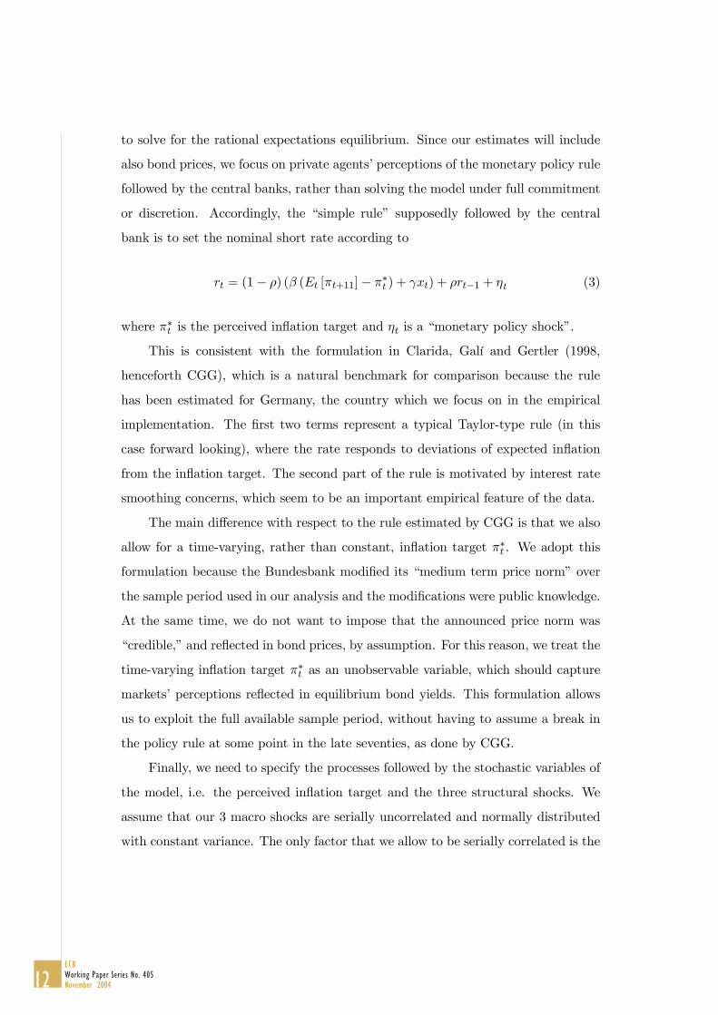
to solve for the rational expectations equilibrium. Since our estimates will include
also bond prices, we focus on private agents’ perceptions of the monetary policy rule
followed by the central banks, rather than solving the model under full commitment
or discretion. Accordingly, the “simple rule” supposedly followed by the central
bank is to set the nominal short rate according to
� = (1− ) (� (�� [��+11]− �∗� ) + ���) + �−1 + �� (3)
where �∗� is the perceived inflation target and �� is a “monetary policy shock”.
This is consistent with the formulation in Clarida, Galí and Gertler (1998,
henceforth CGG), which is a natural benchmark for comparison because the rule
has been estimated for Germany, the country which we focus on in the empirical
implementation. The first two terms represent a typical Taylor-type rule (in this
case forward looking), where the rate responds to deviations of expected inflation
from the inflation target. The second part of the rule is motivated by interest rate
smoothing concerns, which seem to be an important empirical feature of the data.
The main difference with respect to the rule estimated by CGG is that we also
allow for a time-varying, rather than constant, inflation target �∗� . We adopt this
formulation because the Bundesbank modified its “medium term price norm” over
the sample period used in our analysis and the modifications were public knowledge.
At the same time, we do not want to impose that the announced price norm was
“credible,” and reflected in bond prices, by assumption. For this reason, we treat the
time-varying inflation target �∗� as an unobservable variable, which should capture
markets’ perceptions reflected in equilibrium bond yields. This formulation allows
us to exploit the full available sample period, without having to assume a break in
the policy rule at some point in the late seventies, as done by CGG.
Finally, we need to specify the processes followed by the stochastic variables of
the model, i.e. the perceived inflation target and the three structural shocks. We
assume that our 3 macro shocks are serially uncorrelated and normally distributed
with constant variance. The only factor that we allow to be serially correlated is the
12ECBWorking Paper Series No. 405November 2004

unobservable inflation target, which will follow an AR(1) process
�∗� = ���∗�−1 + ���� (4)
where ���� is a normal disturbance with constant variance uncorrelated with the
other structural shocks.
2.2 A general macroeconomic set-up
In order to solve the model we write it in the general form
X1��+1
��X2��+1
=H X1��X2��
+K� +
ξ1��+1
0
� (5)
where X1 is a vector of predetermined variables, X2 includes the variables which
are not predetermined, � is the policy instrument and ξ1 is a vector of independent,
normally distributed shocks (see the appendix for the exact definitions of all these
variables in our example). The short-term rate can be written in the feedback form
� = −F X1��X2��
(6)
This linear structure is nevertheless general enough to accommodate a large
number of standard macroeconomic models, potentially much more detailed than
the one we adopt here. The main restriction we impose, for simplicity, is that only
the short-term interest rate, which is controlled by the central bank, affects the
macro economy, whereas longer rates do not.
The solution of the (5)-(6) model can be obtained numerically following stan-
dard methods. We choose the methodology described in Söderlind (1999), which is
based on the Schur decomposition. The result are two matricesM and C such that
X1�� =MX1��−1+ξ1�� and X2�� = CX1��.5 Consequently, the equilibrium short term
5The presence of non-predetermined variables in the model implies that there may be multiplesolutions for some parameter values. We constrain the system to be determinate in the iterativeprocess of maximizing the likelihood function.
13ECB
Working Paper Series No. 405November 2004

interest rate will be equal to � = ∆0X1��, where ∆0 ≡ − (F1+F2C) and F1 and
F2 are partitions of F conformable with X1�� and X2��. Focusing on the short-term
(policy) interest rate, the solution can be written as
� = ∆0X1��
X1�� = MX1��−1 + ξ1�� (7)
2.3 Adding the term structure to the model
The system (7) expresses the short term interest rate as a linear function of the
vector X1, which in turn follows a first order Gaussian VAR. This structure is
formally equivalent to that on which affine models are normally built. To derive
the term structure, we only need to impose the assumption of absence of arbitrage
opportunities, which guarantees the existence of a risk neutral measure, and to
specify a process for the stochastic discount factor.
Behind this formal equivalence, however, our model has the distinguishing fea-
ture that both the short rate equation and the law of motion of vector X1 have
been obtained endogenously, as functions of the parameters of the macroeconomic
model. This contrasts with the standard affine set-up based on unobservable vari-
ables, where both the short rate equation and the law of motion of the state variables
are postulated exogenously.
This feature also differentiates our approach from Ang and Piazzesi’s (2003).
More specifically, Ang and Piazzesi (2003) still rely on an exogenously postulated
model of the short-term rate, which they interpret as the monetary policy rule.
In any macroeconomic model, however, the dynamics of the short term rate will
be obtained endogenously. We show that this property of macro-models does not
prevent the specification of a dynamic arbitrage-free term structure model. Provided
that one’s favorite macroeconomic model can be cast in the linear (5)-(6) form,
arbitrage-free pricing is possible.
In fact, rather than building the term structure directly on equations (7), we al-
low for the possibility to write bond yields as functions of a different vector, Z�, which
can include any variable in X� or the short term rate. The new vector Z� is defined
14ECBWorking Paper Series No. 405November 2004

as Z� = DX�, whereD is a selection matrix. Obviously, Z� can also be rewritten as a
function of the predetermined vector X1� using the result X2�� = CX1��. This yields
Z� = DX1��, where D is a matrix described in the appendix. Specifically, in the
empirical application, we choose D so that bond yields are expressed as functions
of the levels of the macro variables, rather than of their shocks.
Given the solution equation for the short term interest rate written as a function
of the Z� vector, � = ∆0Z�, we follow the standard dynamic arbitrage-free term
structure literature and define the (nominal) pricing kernel ��+1, which prices all
nominal bonds in the economy, as ��+1 = exp (−�)��+1���, where ��+1 is assumed
to follow the log-normal process ��+1 = �� exp¡−12�0��� − �0�ξ1��+1
¢.
We then make an assumption on the dynamics of ��, the vector of market
prices of risk associated with the underlying sources of uncertainty in the economy.
These have commonly been assumed to be constant (in the case of Gaussian models)
or proportional to the factor volatilities (e.g. Dai and Singleton, 2000), but recent
research has highlighted the clear benefits in allowing for a more flexible specification
of the risk prices (e.g. Duffee, 2002; Dai and Singleton, 2002). We therefore assume
that the market prices of risk are affine in the state vector Z�
�� = �0 + �1Z�� (8)
so that the market’s required compensation for bearing risk can vary with the state
of the economy.
It should be pointed out here that, in a micro-founded framework, the pricing
kernel (or stochastic discount factor) would be linked to consumer preferences, rather
than being postulated exogenously as we do here. The pricing kernel would be
obtained from the intertemporal consumption Euler equation, essentially consisting
of the discounted ratios of marginal utility between two consecutive periods, scaled
by expected inflation in the case of the nominal kernel. In standard consumption-
based formulations of asset pricing models, the prices of risk would be related to
the agents’ risk aversion and to the curvature of the indirect utility function with
respect to the state variables of the problem. We would obtain a micro-founded
15ECB
Working Paper Series No. 405November 2004

pricing kernel if we specified a utility function, set �1 = 0 and restricted �0 to be
consistent with the selected utility function.6
We prefer our exogenous specification (8) for two main reasons. The first is that
we want to employ an empirically plausible formulation and the state-dependent
specification in equation (8) is not straightforward to obtain from first principles.7
The second reason is that, even if we found a sufficiently flexible formulation of the
utility function, the yield premia would always be zero in a log-linearized solution
of the model, such as the one we implicitly adopt here (see also Kim et al., 2003).
Higher order approximations could obviously be employed to deal with this problem,
but they would imply leaving the convenient affine world, in which both the bond
prices and the likelihood can be specified in closed-form.
In the appendix we show that the reduced form (7) of our macroeconomic
model, coupled with the aforementioned assumptions on the pricing kernel, implies
that the continuously compounded yield ��� on an �-period zero coupon bond is
given by
��� = �� +�0�Z�� (9)
where the �� and �0� matrices can be derived using recursive relations. Stacking
6Consider the example of a standard economy populated by a representative household with
utility function over consumption and labour � (��� ��) =�1−�
�
1−� − ��� and production function
� = ���� , where � is a productivity shock such that ln� = � ln�−1 + ��. If prices are fully
flexible, it is easy to show that equilibrium will imply �� = � and, using lower case letters to denote
the natural log of a variable, � = ��+�(�−1) ln
³��
´+ �
�+�(�−1)��.
The (real) stochastic discount factor ����+1 will be given by ����+1 = ���(��+1)��(��)
= � (�+1��)−� .
If we use the definition of the gross interest rate �� as 1��� = �� [����+1], take logs, and writeoutput in terms of its determinants, we obtain
����+1 = −�� − 1
2
µ��
�+ � (� − 1)¶2
�2� − ��
�+ � (� − 1)����+1
where ��+1 is a white noise shock with unit variance.This formulation is entirely analogous to the one used in the paper, i.e. ����+1 = −�� − 1
2�0��� −
�0��1��+1. In this simple model, the (constant) prices of risk are given by
� =��
�+ � (� − 1)��
7Dai (2003) argues that preferences embodying a particular specification of habit formationwould be consistent with pricing kernel that, to a first order approximation, would be of the form(8) with a non-zero �1.
16ECBWorking Paper Series No. 405November 2004

all yields in a vector Y�, we write the above equations jointly as Y� = A+B0Z� or,
equivalently, Y� = A+ B0X1��, where B0 ≡ B0D.
2.4 Maximum likelihood estimation
In order to estimate the model, we need to distinguish first between observable and
unobservable variables in the X� vector. We adopt the approach which is common
in the finance literature and which involves inverting the relationship between yields
and unobservable factors (Chen and Scott, 1993). In our case, the method needs
to be extended to take into account that the observable variables include not just
the yields, Y�, but also some of the non-predetermined variables. We also use the
common approach of assuming that some of the yields are imperfectly measured to
prevent stochastic singularity.
Using the assumption of orthogonality of measurement error shocks and shocks
to the unobservable states, we show in the appendix that the log-likelihood function
to maximize takes the form
£ (θ) = − (� − 1)Ãln |J|+ ��
2ln (2�) +
1
2ln¯ΣΣ0
¯+
�
2ln (2�) +
1
2
�X�=1
ln�2�
!
−12
X�=2
¡X�1��−M�X�
1��−1¢0 ¡ΣΣ0
¢−1 ¡X�1��−M�X�
1��−1¢− 1
2
X�=2
�X�=1
³����
´2�2�
�
where X�1�� are the unobservable variables included in the X1�� vector, �
� are the
measurement error shocks, J is a Jacobian matrix defined in the appendix,ΣΣ0 is the
variance-covariance matrix of the four macroeconomic shocks, �� are the standard
deviations of measurement error shocks, � is the sample size, � is the number of
measurement errors and �� is the number of variables measured without error.8 The
expression for the log-likelihood function above is based on the fact that there is a
one-to-one mapping from the observable variables (yields, output, and inflation) to
the unobservables (X�1�� and �� ), with J being the Jacobian associated with this
8So far, we have not imposed any restrictions on the X1� vector. In the estimation, however,care must be taken to avoid that the unobservable variables included in X1� be linearly dependent.If this were the case, the Jacobian matrix would not be invertible.
17ECB
Working Paper Series No. 405November 2004
mapping.
When, as in the model used by Ang and Piazzesi (2003), there is no feedback
from interest rates to the macro variables, estimation can be performed with a two-
step procedure. In the more general case analyzed here this is not possible and we
must estimate the whole system jointly.
In theory, this is of course preferable. The problem is that the parameter space
is quite large and therefore the optimization problem of maximizing the likelihood
function is non-trivial and time consuming. We employ the method of simulated
annealing, introduced to the econometric literature by Goffe, Ferrier and Rogers
(1994). The method is developed with an aim towards applications where there
may be a large number of local optima.9
One disadvantage of the simulated annealing method is that it does not provide
us with an estimate of the derivatives, evaluated at the maximum, of the likelihood
function with respect to the parameter vector, i.e. � ln (£ (θ)) ��θ0. These deriv-
atives are necessary to compute asymptotic estimates of the variance-covariance
matrix of the parameters. The derivatives could be evaluated numerically, but the
computation would be based on arbitrarily selected step-lenghts �θ, with ensuing
risks of spurious results because of the highly nonlinear fashion in which the para-
meters enter the likelihood function.
To deal with this problem, we rely on analytical results to calculate the Jacobian
� ln (£ (θ)) ��θ0. The evaluation of the analytical derivatives is quite involved. The
key steps are described in the appendix.
9The key parameters of the simulated annealing method were set as follows: �0 = 15; � = 0�9;� = 20. The convergence criterion � was set at � = 1�0� − 8. In a preliminary estimation, thestarting values were taken from CGG’s results (for the policy rule) and from the parameters of anunrestricted VAR in output, inflation, and the short term nominal rate. The estimates reportedin the text correspond to a maximum value of the likelihood function found in a process of 100estimations using simulated annealing, starting from randomized initial values.
18ECBWorking Paper Series No. 405November 2004

3 An application to German data
3.1 Data
Our data set runs from January 1975 to December 1998. The term structure data
consists of monthly German zero-coupon yields for the maturities 1, 3 and 6 months,
as well as 1, 3, and 7 years.10 We assume that the 1-month rate and the 3-year yield
are perfectly observable, while the other rates are subject to measurement error.
Yields have been bootstrapped from on an original Bundesbank dataset of end-of-
month raw prices, coupons and maturities.11
Concerning the macro data, we construct the year-on-year inflation series using
the CPI (all items). For the output gap, we simply follow CGG and detrend the log
of total industrial production (excluding construction) using a quadratic trend. We
only deviate from CGG in constructing the series recursively, so that each datapoint
is obtained by fitting a quadratic trend to the original series up to that point. We
adopt this approach to ensure that our forecast at time � does not rely on information
unavailable at that point in time. Both series refer to unified Germany from 1991
onwards and to West Germany prior to this date. The macroeconomic and term-
structure series are shown in Figure 1.
3.2 Estimation results
To reduce the parameter space in our empirical application, we impose a number of
restrictions on the coefficients of the market prices of risk. In the general set-up, we
showed that the risk prices can be specified as �� = �0 + �1Z�. In our application,
Z� includes the perceived inflation target and contemporaneous and lagged values of
inflation, output and the short term rate. Given Z�, �� can obviously have nonzero
elements only corresponding to time � variables, as lagged variables are no longer
subject to surprise changes. This leaves only four potentially non-zero rows in the �0
and �1 matrices, corresponding to the perceived inflation target, the policy interest
10We do not use 10-year bonds because these are only available without breaks as of April 1986.11The methodology is equivalent to that employed by Fama and Bliss (1987). We wish to thank
Thomas Werner for providing us with the raw data and Vincent Brousseau for bootstrapping theterm structures of zero-coupon rates.
19ECB
Working Paper Series No. 405November 2004

rate, inflation and the output gap. Next, we restrict �1 in the sense of allowing
interactions only between prices of risk of contemporaneous variables, which leaves
us with a 4 × 4 non-zero submatrix in �1. Finally, we follow Duffee (2002) and
set to zero all entries whose elements have a t-statistic lower than 1 in preliminary
estimations.12 As a result, we are left with the following non-zero elements in the
matrices of prices of risk
�� =
�01
�02
�03
�03
+
0 0 �13 �14
�21 �22 �23 0
�31 �32 �33 0
0 �42 0 �44
�∗�
�
��
��
3.2.1 Parameter estimates
Table 1 presents the parameter estimates with associated asymptotic standard errors
(based on the analytical outer-product estimate of the information matrix).
The results are broadly consistent with the evidence of Clarida, Galí and
Gertler (1998) regarding the Taylor rule in Germany and, as far as the other macro-
parameters are concerned, with existing evidence based on structural models or
identified VARs.
For example, our point estimate of the degree of forward-lookingness of infla-
tion (��) is within the range of values found by Jondeau and Le Bihan (2001), who
estimate on German data a Phillips curve based on quarterly data using a variety of
specifications and two different estimation methods. Kremer, Lombardo and Werner
(2003), who estimate a structural macroeconomic model with explicit microfounda-
tions, estimate a much higher value of ��. Their estimate, however, is not directly
comparable to ours due to the fact that they capture the persistence of inflation
through highly persistent exogenous shocks (whereas our shocks are white noise).
A result which casts doubts on the ability of our macro-model to provide an
12These preliminary estimations involved first estimating the model with full 4× 1 �0 and 4× 4�1 matrices. Then, the � parameter with lowest �-statistic (below 1) was fixed at zero. The modelwas reestimated, and again the � parameter with lowest �-statistic was constrained to be zero. Thisprocess was repeated until no � parameters with �-statistics below 1 remained.
20ECBWorking Paper Series No. 405November 2004

accurate characterization of the dynamics of output and inflation in Germany is
that the elasticity of inflation to the output gap is very small (�� = 00004 and
insignificantly different from zero). This is not entirely surprising. Jondeau and Le
Bihan (2001) also find values of �� close to zero for some specification/estimation
method (Kremer, Lombardo and Werner, 2003, calibrate, rather than estimate, this
parameter). Identified VARs estimated at the monthly frequency (e.g. Sims, 1992)
also tend to find a very small and insignificant responses of inflation to, e.g., mone-
tary policy shocks, which is consistent with our results of a very small �� and also
a small ��.
To assess whether our macro-parameter estimates are affected by our inclusion
of term structure information in the model, we re-estimated the macroeconomic
model separately. In order to work with a more conventional set-up, we also elim-
inated the stochastic inflation target from the policy rule and replaced it with the
Bundesbank’s announced price norm. Apart from a small increase in �� from 003
to 006, the other parameter estimates (including ��) were virtually unchanged.
The macro-model performance may be affected by the fact that volatile, monthly
data are noisy and make it harder to identify the link between inflation, output and
interest rates. Another possibility is that our output gap definition, which plays a
crucial role in the analysis, is an imperfect proxy for the theoretical notion of real
marginal costs. Or else, as already emphasized, our 2-variable macro-model may be
too parsimonious to describe German macroeconomic dynamics, which are possibly
affected also by variables such as the exchange rate or, as in Kremer, Lombardo
and Werner (2003), a monetary aggregate. Since our main interest is not that of
finding the macroeconomic model most suited for German policy analysis, we do not
perform further specification search. We only test for a potential missing variable
bias by examining the residuals’ autocorrelation. We find little evidence of serial
correlation in our preferred specification.13
As to the other parameters, the autocorrelation coefficient of the inflation target
13More precisely, looking at the correlograms of the estimated residuals we find no evidence ofstatistically significant first or higher order correlation in the output and inflation equations.
21ECB
Working Paper Series No. 405November 2004

process is very close to 1.14 Concerning the term structure, our estimates of the
standard deviations of the measurement errors are between 23 basis points for the
3-month rate and 28 basis points for the other yields. These values are broadly in
line with the results of models based solely on unobservable factors and also those of
an unrestricted VAR including inflation, the output gap and the bond yields.15 The
standard errors of the 1-month and 3-month rate equations of the VAR are equal
to 43 and 32 basis points, respectively, compared to 48 and 23 in our model; for 1-
year and 7-year yields, the VAR equations have a standard error of 29 and 24 basis
points, respectively, compared to 28 and 28 in our model. Obviously, our model
has the advantage of describing, at the same time, the yields for all other possible
maturities (and it also does better than the VAR at fitting output and inflation).
Finally, one of the benefits of our model is that of providing us with a measure
of the central bank’s inflation target as reflected in the prices of long term bonds.
One of the tests of the model is therefore to check whether the filtered series “looks”
reasonable. For this purpose, Figure 2 compares it to the Bundesbank medium term
price norm.16 The two series are quite close to each other in the volatile seventies
and in the sharp decline of the beginning of the eighties. A large discrepancy can be
observed mostly at the beginning of the nineties, when the estimated target increases
sharply while the price norm remains unchanged. The increase in the estimated tar-
get is, however, not unreasonable, as it coincides with an increase in actual inflation
following the expansionary policies that accompanied German unification.17 At the
same time, we cannot exclude the possibility that the variability of the target may be
overestimated in order to induce inflation persistence present in the data, which our
stylized model may be unable to capture endogenously. Nevertheless, the perceived
inflation target is less variable than actual inflation, both in terms of its sample
14This parameter is constrained to be strictly smaller than 1 in the estimation.15The VAR is estimated over the same sample period and includes 3 lags of the variables.16Until 1981 and from 1997 to 1998, the Bundesbank actually announced a range, rather a point
value, for the price norm. In these years, the mid-point of the range is displayed in Figure 2. Novalues were announced pre-1976 and in 1979.17 In spite of the unchanged price norm, this may have sparked fears of a waning in the Bundesbank
anti-inflationary determination because of domestic — due to unification — and European-wide — dueto the impact of any monetary policy tightening on ERM partner countries — political pressures (seeIssing, 2003, for a concise account of the Bundesbank’s policy at the time of German unification).
22ECBWorking Paper Series No. 405November 2004
standard deviation and of its minimum and maximum sample values.
3.2.2 Impulse response functions
Our structural model allows us to compute impulse response functions of macro
variables and yields to the underlying macro shocks.
Figures 3 to 6 show the impulse responses of selected variables to the structural
shocks. The responses of the macroeconomic variables and of the short term interest
rate are broadly in line with existing VAR evidence based on German (monthly)
data and we will not delve on them here. We concentrate instead on the responses
of yields.
We start from Figure 3, which displays the impulse responses to a shock to the
perceived inflation target, which increases on impact by approximately 02 percent-
age points. The shock is obviously expansionary and very persistent, due to the high
serial correlation of the inflation target process. The response of the yield curve is
an almost parallel and very persistent upward shift at all maturities, except the very
short ones (which move slowly because of the high interest rate smoothing coefficient
in the policy rule). The size of the shift corresponds roughly to that of the initial
inflation target shock and it is significantly different from zero for maturities around
1-year.
Figure 4 shows the effect of a 45 basis points increase in the 1-month interest
rate because of a monetary policy shock (the disturbance ��). The response of the
yield curve is decreasing in the maturity of yields, which factor in the slow return
to baseline of the policy rate. Hence, a monetary policy shock tends to cause a
statistically significant change in the slope of the yield curve. The shape of this
response is qualitatively similar to that obtained by Evans and Marshall (1996) for
the US.
An inflation shock, shown in Figures 5, tends to increase the curvature of the
yield curve. Yields move little and slowly at the short end, more around the 1-
year maturity, then little again at the long end. While statistically significant for
maturities below 7 years, the responses appear to be very small from a quantitative
viewpoint.
23ECB
Working Paper Series No. 405November 2004

Finally, Figures 6 shows the impulse responses to an output shock. Due to
the small policy response, the yield curve increases little, but significantly, over
maturities up to 1 year. Yields on 3 and 7-year bonds, however, fall as a result of
the shock and in spite of the fact that the response of the short-term rate always
remains above the baseline. This surprising pattern is to a large extent shaped by
the dynamics of risk premia.
3.3 Macro shocks and risk premia
Another advantage of our joint treatment of macroeconomics and term-structure
dynamics is that we are able to derive the impulse response of theoretical risk premia
to macro shocks, including the monetary policy shock. These are shown in Figure
7.
The inflation target shock is immediately followed by an increase of the yield
premium for maturities up to 4 years, with a peak effect of 10 basis points at the
1-year maturity. The premium then turns negative for longer maturities. Such
increase in the yield premium is highly significant from an economic viewpoint, as it
plays a large quantitative role in shaping the total yield response displayed in Figure
3.
The monetary policy shock gives rise to a large fall, on impact, at the short
end of the term structure of yield premia, thus reducing significantly the size of
the impact response of the yields. The impact response of the 1-year yield to the
monetary policy shock, for example, would increase by one half if yield premia were
set equal to a constant.
Similar considerations hold for the impact response of yield premia to inflation
and output shocks. The latter is notable, since the premia embody most of the
action in the response. The impact response of the 7-year rate, for example, would
change sign and essentially maintain the same in absolute value, if risk premia were
constant.
We conclude that, in general, the dynamics of yield premia have a nonnegligible
effect on the impulse responses of yields to all macroeconomic shocks. An interpre-
tation of the yield responses based on the expectations hypothesis may therefore be
24ECBWorking Paper Series No. 405November 2004
significantly biased.

The general features of the yield premia are that their level and volatility are
increasing in maturity. The premia also tend to be decreasing over the sample in
parallel to the fall in inflation, but then shoot up again, temporarily, in 1992-93. To
investigate their determinants more closely (using equation (15) in the appendix), we
can decompose the premia in the components due to risk of changes in the inflation
target, in the short-term rate, in inflation and in the output gap.18 We focus here
on the most important components for 1- and 7-year maturities.
The most striking outcome of this decomposition is that premia linked to in-
flation risk are almost perfectly constant over time and negligible in size across
maturities. Even at their peaks, they never reach the level of 10 basis points. This
number should be compared, for example, to the maximum level of 1 percentage
point reached by the premium due to output gap uncertainty for 7-year bonds.
Variations in yield premia arise by and large from fluctuations in the other three
variables, with an importance that changes across maturities. Figure 8 shows that
at the 1-year horizon, the largest fraction of the time-varying yield premium is due
to interest rate risk, i.e. the possibility of monetary policy surprises. The price of
interest rate risk, in turn, is decreasing in the level of the interest rate: when the
latter is very high, yield premia are lower than average and 1-year bonds appear to be
a very appealing form of investment; when interest rates are low, on the contrary, the
risk of unexpected changes in the short-term rate has a higher price and 1-year bond
command a higher than average premium. The second most important component
of the time varying yield premium at 1-year maturities is inflation target risk. The
target premium is increasing in the level of the inflation target. A high inflation
target makes 1-year bonds riskier and increases the premium investors require to
hold them.
At the long 7-year horizon, Figure 8 shows that the time varying component
of the yield premium is almost entirely due to inflation target risk until the end of
18This decomposition is not exact, because the term premium is also affected by the lags ofinflation, output and the interest rate. We disregard these additional effects for two reasons. First,given our assumption on the prices of risk ��, they are due to convexity effects, rather than a purerisk premium. Second, they are quantitatively minor.
25ECB
Working Paper Series No. 405November 2004

1988. At this maturity, the inflation target premium is negatively correlated with
the level of the inflation target. When the target is high, the yield premium is lower
than average and investors are relatively more willing to hold 7-year bonds. This
may be taken as a signal of investors’ confidence in the ultimate return to a low
inflation target environment. As of 1989, with inflation and the policy interest rate
increasing after the German unification and the recession of 1992-93 ensuing, the
variable yield premium becomes significantly affected also by output gap risk. In
other words, booms tend to make investors more willing to hold long term bonds,
while investors require a larger bond premium during recessions.
4 Forecasting
The forecasting performance is a particularly interesting test of our macroeconomic-
based term-structure model. Due to the relatively large number of parameters that
needs to be estimated, the model could be expected to perform poorly with respect to
more parsimonious representations of the data. In fact, the random walk model has
been shown to provide yield forecasts that are particularly difficult to beat (Duffee,
2002). An important test of our model is therefore to check whether the information
contained in macro variables can improve the performance of a standard essentially-
affine model including only term-structure information. For completeness, we also
check whether the inclusion of yields in the information set can improve the perfor-
mance of the macro-only model in terms of forecasting the macro variables.
The forecasting tests for macroeconomic variables and yields are presented in
turn in the next two sections. Our results suggest that term structure information
helps little in forecasting macroeconomic variables. Our structural framework in-
cluding macroeconomic variables does, however, help to forecast yields. The out-of-
sample forecasting performance of our model up to 12-month ahead is almost always
superior to all the alternatives we consider, and the difference is often statistically
significant.
26ECBWorking Paper Series No. 405November 2004

4.1 Do yields help to forecast macroeconomic variables?
Given the imperfect ability of our macroeconomic model to describe the joint dynam-
ics of German macroeconomic variables, we do not expect it to be very successful in
forecasting inflation and the output gap. This is consistent with existing evidence.
In a thorough study of inflation forecasting in the G7 countries, for example, Canova
(2002) concludes that theory-based models are not always better than atheoretical
univariate models.
Our test on macroeconomic variables is therefore very focused on assessing
whether including yields in the analysis can help in forecasting. We evaluate the
out-of-sample forecasting performance of our macro-term structure model (HTV)
relative to the macro-only model (HTV-M) used in Section 3.2.1. Both models are
estimated over the period February 1975 - December 1994, and output gap and
inflation forecasts up to 12 months ahead are produced for each month over the
period January 1995 to December 1998. We update the information set each month,
but we do not reestimate the model. Instead, we rely on the estimates up until end-
1994. We choose this approach to limit the computational burden of the exercise
(this applies in particular for the yield forecasts in the next section). All results are
therefore based on the same estimated parameters.
The root mean squared errors (RMSEs) are presented in Table 2. Lower val-
ues of the RMSE denote better forecasts, and the best forecast at each horizon
is highlighted in bold. The table shows that the full model including term struc-
ture information and the stochastic inflation target does marginally better than the
macro-only model at forecasting inflation. The latter model, however, prevails as
far as output forecasts are concerned.
We conclude that yields are unlikely to provide useful information for macroeco-
nomic forecasting within our framework. This result may be due to our assumption
that long term yields do not affect the dynamics of inflation and the output gap.
27ECB
Working Paper Series No. 405November 2004

4.2 Do macroeconomic variables help to forecast yields?
To assess the yields forecasting performance of our model, we compare it to a number
of benchmarks.
The first is the random walk. In addition, we also consider forecasts based
on three other models. One is a canonical �0 (3) essentially affine model based on
unobservable factors.19 Provided that risk premia are specified to be linear functions
of the states, Duffee (2002) finds this model most successful in the class of admissible
affine three factor models in terms of forecasting US yields. Apart from providing
a benchmark for comparison, our results on the �0 (3) model are of independent
interest, since they highlight the performance of this model on a different data-set.
The second model we take into account is the Ang and Piazzesi (2003) model, which
we reestimate on our data-set. Based on Ang and Piazzesi’s results, we use their
favorite “Macro model” in this exercise, i.e. a model in which the interest rate
responds to current inflation and output gap, as well as to 3 unobservable factors. A
potentially important difference in our application of their model, however, is that we
use inflation and the output gap directly in the estimation, rather than the principal
components of real and nominal variables employed by Ang and Piazzesi (2003),
thereby facilitating comparison to our results. Finally, we use an unrestricted VAR
including all the variables in our structural model, in order to gauge the importance
of structural and no-arbitrage restrictions to improve the performance of our model.
As in the previous section, the out-of-sample forecasting performance of the
models is based on estimates up to end-1994, and 1- to 12-step ahead forecasts
are produced for all yields used in the estimation over the period January 1995 to
December 1998. The RMSEs of this forecast evaluation exercise are summarized
in Tables 3, with the best forecast at each maturity/horizon highlighted in bold.
The exercise shows that our model performs better than the alternatives for all
maturities, at least beyond the very shortest forecast horizon. In particular, our
model beats the predictions of the random walk benchmark in almost all cases. Table
4, which displays the trace MSE statistic − a multivariate summary measure of the
19For a definition of the 0 (3) class of affine models, see Dai and Singleton (2000).
28ECBWorking Paper Series No. 405November 2004

forecasting performance across yields for each horizon − confirms this picture.20
To understand the reasons for this success, compare first the performance of the
�0 (3) model in Table 3 to that of the VAR. The former model includes no-arbitrage
restrictions and, as a result, it appears to be more efficient at forecasting long yields,
especially at longer forecasting horizon. The �0 (3) model, however, is not always
superior to the VAR, which is a first suggestion that macroeconomic information
could be important in forecasting yields. The AP may be expected to improve the
performance of the �0 (3) model, because it includes macroeconomic information on
top of the no-arbitrage restrictions. The AP model includes, however, a very large
number of parameters to estimate, since it is based on a reduced-form representation
of the macroeconomic variables. This may be the cause for its less satisfactory
performance over forecasting horizons beyond 1 month. Its good performance in
1-step ahead forecasts is, incidentally, consistent with the results reported by Ang
and Piazzesi (2003). Our model appears to strike a good balance in incorporating
macroeconomic information without becoming overparameterized.
Concerning, more specifically, the market prices of risk, a crucial role in affecting
the forecasting performance of our model is played by risk premia associated to
inflation target risk. If we re-estimate our model restricting to zero the elements
in equation (8) associated to the inflation target, i.e. �21 and �31, the forecasting
performance of the model worsens dramatically, especially for long maturities. This
appears to be consistent with the evidence on the main components of the risk
premia presented in section 3.3.
In order to formally test the out-of-sample yield forecasting performance of our
model, we apply White’s (2000) “reality check” test. This test, which builds on the
work of Diebold and Mariano (1995) and West (1996), involves examining whether
the expected value of the forecast loss (e.g. the squared forecast error) of one or
several models is significantly greater than the forecast loss of a benchmark model.
We choose this test mainly because, in contrast to many other forecast performance
20The trace MSE statistic has been used, for instance, by Christoffersen and Diebold (1998). Foreach forecast horizon, it is simply computed as the trace of the covariance matrix of the forecasterrors of all yields considered. Hence, a lower trace MSE statistic signals more accurate forecastsacross yields.
29ECB
Working Paper Series No. 405November 2004

tests, it tests for superior predictive ability rather than equal predictive ability.
Moreover, White’s test allows us to examine whether a specific model is significantly
outperformed by any model among a number of alternatives, whereas other tests
typically do not permit this.
We implement the test in two ways. First, we take our model as the benchmark
and ask whether any of the four alternative models is able to produce forecasts that
are significantly superior to our model across each of the five maturities and 12
forecast horizons considered. We found that in only 3 out of the 60 cases could we
reject the null hypothesis that none of the four models is better than our model.21
While encouraging, this result does not necessarily imply that our model is superior
to the alternatives. To test this, we instead turn around the null hypothesis and
proceed to test for superior predictive ability of our model vis-à-vis each of the
four alternative models separately. In other words, we implement four pairwise
comparisons, where each of the four alternative models are used as the benchmark
model against the HTV model. The results are displayed in Table 5, where bold
figures indicate rejection of the null that our model does not have superior predictive
ability compared to the benchmark used, at the 5% level. In over 60% of the cases we
reject the null, meaning that for most of the combinations of maturities and forecast
horizons considered here, the forecasting performance of our model is significantly
better than the alternatives. Looking at the results in more detail, we see that,
somewhat surprisingly, the VAR model seems to be harder to beat than the other
alternatives, although for longer horizons and maturities the HTVmodel consistently
outperforms the VAR. With respect to the performance of our model at different
forecast horizons, we seem to do roughly equally well across all horizons, except for
the one-month ahead case, where the null is rejected less often.
We therefore conclude that the inclusion of macroeconomic variables within
a structural framework contributes to sharpening our ability of forecasting yields
accurately out of sample. The improvement is due both to the inclusion of addi-
tional information in the model, and to the structural restrictions imposed on its
21These results are not reported, but are available on request.
30ECBWorking Paper Series No. 405November 2004
macroeconomic and term structure sections.

5 Expectations hypothesis tests
According to the expectations hypothesis, the yield on an �-period zero-coupon
bond should increase when the spread between the same yield and the short term
rate (the “slope of the yield curve”) widens. In fact, the projection of the yield
change ��−1�+1 − ��� on the yield spread (��� − �) � (�− 1) should yield a coefficient
of 1. A number of empirical tests of this implication of the theory have, however,
found a negative relationship. This pattern represents a puzzle for the expectations
hypothesis, and it appears to be particularly clear for United States data. The
relevant regression coefficient can be as big as −5 for 10-year bonds, according toe.g. Campbell and Shiller (1991), while the expectations hypothesis predicts a value
of one for all maturities.
One interpretation of these results is that the large deviation from 1 in the
estimated coefficient on the yield spread is due to large and time varying risk pre-
mia (not permitted by the expectations hypothesis). Using a highly stylized model,
McCallum (1994) conjectures that an exogenous, stochastic term premium is, in
principle, capable of causing deviations from 1 in the slope coefficient of the afore-
mentioned regression. The actual size of the deviation will depend on both the
stochastic properties of the term premium (see also Roberds and Whiteman, 1999)
and the monetary policy rule followed by the central bank. These papers, however,
work by “reverse engineering.” Given the results of projections of the yield change on
the yield spread, they derive the properties that risk premia should have to explain
those results. This is different from deriving the risk premia from a certain model
and checking ex-post if they are capable of solving the expectations puzzle.
In this section, we follow the latter strategy. We do not test if the yield premia
consistent with our model are capable of solving the expectations puzzle for some
parameter values. This is likely to be the case, given that our model includes a
relatively flexible specification of the market prices of risk. We ask instead a more
stringent question, namely whether the premia generated by our model can solve
31ECB
Working Paper Series No. 405November 2004

the expectations puzzle for the specific set of parameter values which maximizes the
likelihood.
In so doing, we follow closely Dai and Singleton (2002) who ask the same ques-
tion within a number of dynamic affine term structure models based on unobservable
factors. More specifically, we ask whether the model-implied, population coefficients
�� in the regression
��−1�+1 − ��� = ��� �+ �� (��� − �) � (�− 1) + ! "#�$% (10)
match the values obtained from an OLS regression on actual yield data. The pop-
ulation coefficient are obtained assuming that the model parameters are true and
then deriving the �� coefficients analytically based on the stochastic properties of
the model.22 Following Dai and Singleton (2002), we also examine the small-sample
counterparts of these coefficients. Some correction for small sample bias is desirable
because of the persistent nature of yields. For this purpose, we generate 1000 sam-
ples of the same length of our data (287) and calculate the mean estimate of the ��
coefficients.
Dai and Singleton (2002) denote the above test as LPY (i). LPY (i) is a test of
the capacity of the model to replicate the historical dynamics of yields as generated
by a combination of the dynamics of risk premia and expectations of future short
rates. As already emphasized, a successful model should be capable of generating
the negative intercept coefficient of Campbell and Shiller-type regressions.
In addition to LPY (i), Dai and Singleton (2002) also suggest running a sec-
ond sort of test, defined as LPY (ii), which focuses on the realism of the dynamic
properties of risk premia. If the model captures these dynamics well, a Campbell
and Shiller-type regression based on risk-premium-adjusted yield changes should re-
cover the coefficient of unity consistent with the expectations hypothesis. LPY (ii)
22This amounts to evaluating analytically �� ≡� �(��−1
�+1 −��� �(��
� −��)�(�−1))���((��
�−��)�(�−1))
.
32ECBWorking Paper Series No. 405November 2004

therefore tests that the sample coefficient �∗� in the regression
��−1�+1 − ��� + !���� (�− 1) = ��� �+ �∗� (��� − �) � (�− 1) + ! "#�$% (11)
is equal to its population value of 1 (in the above regression, !��� is the excess holding
period return !��� ≡ ��
£ln¡&�−1�+1 �&
��
¢− �¤— see appendix).
Dai and Singleton (2002) show that an affine 3-factor model with Gaussian in-
novations and including a risk-premium specification of the type suggested by Duffee
(2002) scores extremely well in terms of both LPY (i) and LPY (ii). Our model also
includes a flexible specification of the risk-premium as in Duffee (2002). Unlike in
pure finance models, however, our risk-premia are partly functions of observable vari-
ables, namely output and inflation. This feature represents an additional constraint,
which makes the LPY tests more stringent than in the pure finance literature.
5.1 LPY (i)
Since the evidence on Campbell and Shiller-type regressions based on European data
is less compelling than for the US (e.g. Hardouvelis, 1994, Gerlach and Smets, 1997,
Bekaert and Hodrick, 2001), we start by replicating Campbell and Shiller’s analysis
on our data. The results of the sample estimates of equation (10) are shown in
Figures 9 and 10 as dots under the label “Sample”. Consistently with the puzzle,
the estimated intercept coefficient is always negative and decreasing in maturity. We
confirm, however, that the puzzle appears less severe for German yield data: the
estimated coefficient hovers around −07 for 7-year yields, compared to a value ofless than −3 reported by Dai and Singleton (2002) for US 7-year yields.
In Figure 9 we show the results of the LPY (i) test. The population coefficients
follow quite closely the pattern of the sample coefficients, although less so for short
maturities. The population coefficients also have the downward sloping feature em-
phasized also by Dai and Singleton. The small-sample values of the �� coefficients
(labelled “Model-implied MC” in Figure 9 and drawn together with 95% confidence
bands of their small-sample distribution) confirm and strengthen this result. Our
model appears to match strikingly well the pattern of the sample coefficients for
33ECB
Working Paper Series No. 405November 2004
essentially all maturities included in the regression.

The success of the model in matching LPY (i) depends crucially on our assump-
tions related to the market prices of risk. Our parameterization of the �1 matrix
permits variations of the prices attached to the various sources of risk depending
on the level of the state variables of the model. For example, the risk premium
required for the possible occurrence of inflation target shocks varies with the levels
of inflation and the output gap (see the first row of the �1 matrix). In fact, it turns
out that the statistically significant dimension of the inflation target premium is not
related to the occurrence of “own shocks” (the first element in the matrix is zero).
What matters is whether inflation and the output gap are high when the target is
also high because of past inflation target shocks.
In specifications not allowing for such interactions — for example if the �1 matrix
were diagonal — we experienced a worsening of the the performance of our model
in terms of the LPY tests. The importance of the interactions generated by the
off-diagonal terms in the �1 matrix is related to the fact that these increase the
persistence of the yield premia. Once the premium related to inflation target shocks
has gone up, it will possibly remain high not only because of the persistence of the
inflation target, but also because of increases in the output gap or inflation driven
by any other shock in the system. The persistence of yield premia, in turn, is crucial
to generate significant deviations in the yields levels from the values consistent with
the expectations hypothesis.
5.2 LPY (ii)
Figure 10 shows the results of the LPY (ii) tests. Once again, the model does
remarkably well in fitting the data. The risk-premium correction always goes in
the right direction and the model can generate a coefficient very close to unity for
maturities of 4 years or longer.
For shorter maturities the model does less well, but we still recover coefficients
that are positive and larger than 0.5, which is a dramatic improvement with respect
to the implications of the expectations hypothesis. The reduced degree of success of
the model at the short end of the yield curve is also consistent with standard results
34ECBWorking Paper Series No. 405November 2004

that 3-factor models are unable to capture short-lived money-market dynamics and
that a fourth factor may be necessary for this purpose. Alternatively, such dynamics
may be captured allowing for jumps in the short-term rate, as in Piazzesi (2003).
To summarize, our model appears to do as well as the essentially affine �0 (3)
class in tests of the expectations hypothesis, in spite of the further constraints im-
posed by the dependence of risk premia on observed variables. The results of LPY (i)
are very positive, in that the model can replicate the estimated coefficient of Camp-
bell and Shiller-type regressions at all maturities. The test of LPY (ii) are also
positive, and especially so for long maturities.
6 Conclusions
This paper presents a general set-up allowing to jointly model and estimate a
macroeconomic-plus-term-structure model. The model extends the term-structure
literature, since it shows how to derive bond prices using no-arbitrage conditions
based on an explicit structural macroeconomic model, including both forward-looking
and backward-looking elements. At the same time, we extend the macroeconomic
literature by studying the term structure implications of a standard macro model
within a dynamic no-arbitrage framework.
In an empirical application, we show that there are synergies to be exploited
from current advances in macroeconomic and term-structure modelling. The two
approaches can be seen as complementary and, when used jointly, give rise to sensible
results. Notably, we show that our estimates of macroeconomic parameters, that are
partly determined by the term-structure data, are consistent with those that would
be estimated using only macroeconomic information. At the same time, our model’s
explanatory power for the term-structure is comparable to that of term-structure
models based only on unobservable variables.
We assess the performance of our model mainly along two dimensions: fore-
casting and ability to solve the expectations hypothesis puzzle.
While yields do not seem to provide useful additional information in forecasting
macroeconomic variables, our model performs very well in forecasting yields. We
35ECB
Working Paper Series No. 405November 2004

argue that this is due to both the inclusion of macroeconomic variables in the infor-
mation set and to the imposition of a large number of no-arbitrage and structural
restrictions.
Our macro-based term-structure model can also match features of yield curve
data which represent a puzzle for the expectations hypothesis. These results confirm
that the dynamics of stochastic risk premia are important determinants of yield
dynamics, and that all such dynamics can be ultimately reconducted to underlying
macroeconomic dynamics within a consistent framework.
36ECBWorking Paper Series No. 405November 2004

Acknowledgements: We wish to thank Gianni Amisano, Greg Duffee, Ivan
Paya, Glenn Rudebusch, Frank Schorfheide, Ken Singleton, Paul Söderlind, Lars
Svensson, and an anonymous referee, as well as seminar participants in the SIEPR-
FRBSF 2003 Conference on “Finance and Macroeconomics,” the University of Bres-
cia Conference on “Macroeconomic issues in the EMU,” the EFA2003 Meetings, the
EEA2003 Meetings, the MMF2003 Conference and the PIER-IGIER Conference on
“Econometric Methods in Macroeconomics and Finance,” for helpful comments and
suggestions. Remaining errors are our sole responsibility. The opinions expressed
are personal and should not be attributed to the European Central Bank.
37ECB
Working Paper Series No. 405November 2004
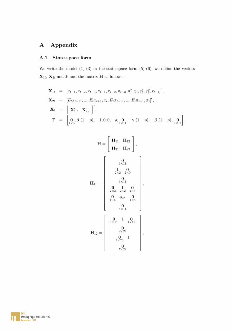
A Appendix
A.1 State-space form
We write the model (1)-(3) in the state-space form (5)-(6), we define the vectors
X1�, X2� and F and the matrix H as follows:
X1� = [��−1� ��−2� ��−3� ��−1� ��−2� ��−3� �∗� � ��� ��� � �
�� � �−1]
0 �
X2� = [����+11� �����+1� �������+11� � ����+1� ��]0 �
X� =hX01�� X02��
i0�
F =
·01×6� � (1− ) �−1� 0� 0�− � 0
1×11�−� (1− ) �−� (1− ) � 01×11
¸�
H =
H11 H12
H21 H22
�
H11 =
01×11I2×2 0
2×90
1×1102×3 I
2×2 02×6
01×6 ��∗ 0
1×40
4×11
�
H12 =
01×11 1 0
1×120
2×240
1×23 1
07×24
�
38ECBWorking Paper Series No. 405November 2004

H21 =
−12(1−��)��
ζ0� 01×6 −
12��
0
011×11
01×3 −
12(1−��)��
δ0� 01×2 −
12��
01×2
011×11
�
H22 =
− 11×11
12��−12 ���
01×11
I11×11 0
11×130
1×11 −12����
− 11×11
12��
011×12 I
11×11 011×1
�
where ζ� = [��1� ��2� ��3]0 and δ� = [��1� ��2� ��3]0,
Finally, we define K =
·0
1×10 1 12 ���
01×23
¸0and ξ�+1 =
·ξ01��+1� 0
1×24
¸0,
where ξ1��+1 =·01×6� ��
∗��+1� ����+1� �����+1� �
����+1� 0
¸0. We can therefore write the
system as
X�+1 = QX� + ξ�+1 (12)
where Q ≡H−KF.
A.2 Bond prices
For the pricing of bonds, we work with the transformed vector Z� defined as Z� =
[��−1� ��−2� ��−3� ��−1� ��−2� ��−3� �∗� � �� ��� ��� �−1]0. Using the solutionX2�� = CX1��,
Z� can be written as Z� = DX1��, where D is
D ≡
µI7×7� 07×4
¶−FGC{24��}
C{12��}µ0
1×10� 1
�
G ≡hI11 C0
i0and C{���} denotes row ' of the matrix C
39ECB
Working Paper Series No. 405November 2004

Given the definition of � and (�+1, the pricing kernel ��+1 = exp (−�) ��+1��
can be written as
��+1 = exp
µ−∆0
Z� − 12�0��� − �0��1��+1
¶� (13)
where we used � =∆0Z� with ∆
0=
·01×7� 1� 01×3
¸.
We know that this set-up will deliver bond prices that are exponential affine
functions of X1��. Since Z� is an affine transformation of X1��, we can write the bond
prices as
&�� = exp¡�� + �0
�Z�
¢(14)
where the coefficients �� and �� have to be determined.
Note first that the price of a one-period bond at time � is &1� = �� [��+1] =
exp¡−∆0Z�
¢, so that �1 = 0 and �1 = −∆. We can now use the pricing kernel
(13) and the postulated form of bond prices (14) to rewrite the equation for the
price of an (�+ 1)-period bond &�+1� = ��
£��+1&
��+1
¤as
&�+1� = exp
µ�� − �0�DΣ�0 +
1
2�0
�DΣΣ0D0�� +
³�0�DMD
−1 −∆0 − �0�DΣ�1
´Z�
where we also used the properties of a lognormal variable �1� such that� [exp ($+ )�1�+1)] =
exp¡$+ 1
2)2*$ [�1�+1]
¢. The bond-pricing coefficients for any maturity � can there-
fore be found using the recursion
��+1 = �� − �0�DΣ�0 +1
2�0
�DΣΣ0D0���
�0�+1 = �0�D
³MD
−1 −Σ�1´−∆0
�
initialized at �1 = 0 and �1 = −∆.
A.3 Likelihood function
To implement ML estimation of the model, we first partition the state vector X1��
into a vector X�1�� that includes only unobservable variables and a vector X
�1�� of
observable variables. Similarly, we define a vector X�2�� of observables from X2��.
40ECBWorking Paper Series No. 405November 2004
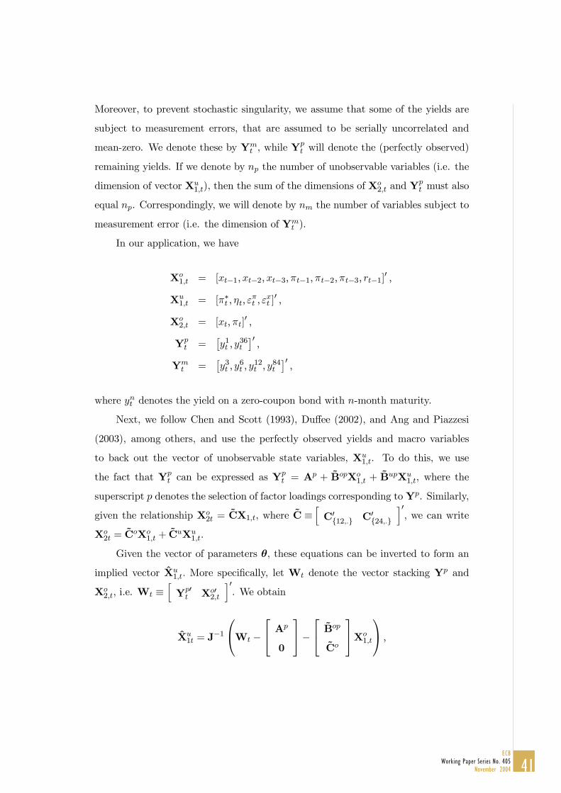
Moreover, to prevent stochastic singularity, we assume that some of the yields are
subject to measurement errors, that are assumed to be serially uncorrelated and
mean-zero. We denote these by Y� , while Y
�� will denote the (perfectly observed)
remaining yields. If we denote by �� the number of unobservable variables (i.e. the
dimension of vector X�1��), then the sum of the dimensions of X
�2�� and Y
�� must also
equal ��. Correspondingly, we will denote by � the number of variables subject to
measurement error (i.e. the dimension of Y� ).
In our application, we have
X�1�� = [��−1� ��−2� ��−3� ��−1� ��−2� ��−3� �−1]0 �
X�1�� = [�∗� � ��� �
�� � �
�� ]0 �
X�2�� = [��� ��]
0 �
Y�� =
£�1� � �
36�
¤0�
Y� =
£�3� � �
6� � �
12� � �84�
¤0�
where ��� denotes the yield on a zero-coupon bond with �-month maturity.
Next, we follow Chen and Scott (1993), Duffee (2002), and Ang and Piazzesi
(2003), among others, and use the perfectly observed yields and macro variables
to back out the vector of unobservable state variables, X�1��. To do this, we use
the fact that Y�� can be expressed as Y
�� = A� + B��X�
1�� + B��X�
1��, where the
superscript & denotes the selection of factor loadings corresponding to Y�. Similarly,
given the relationship X�2� = CX1��, where C ≡
hC0{12��} C0{24��}
i0, we can write
X�2� = C
�X�1�� + C
�X�1��.
Given the vector of parameters θ, these equations can be inverted to form an
implied vector X�1�� More specifically, let W� denote the vector stacking Y� and
X�2��, i.e. W� ≡
hY�0
� X�02��
i0. We obtain
X�1� = J
−1W� −
A�
0
− B��
C�
X�1��
�
41ECB
Working Paper Series No. 405November 2004

where the Jacobian term is given by
J ≡ B��
C�
Finally, given the vector X�1�� implied yields for the remaining � bonds can be
computed using Y� = A
+ B�X�1��+ B
�X�1��, where the superscript � denotes
the selection of factor loadings corresponding to Y In general, these implied yields
will not exactly correspond to the observed yields. The difference produces the
vector of measurement errors, u� = Y� −Y
� , which is assumed to have a constant
diagonal variance covariance matrix with element " given by �2��.
To compute the log-likelihood value, we start from the knowledge that the
one-period ahead conditional distribution of the unobservable state variables has
a multivariate normal distribution +X�1
¡X�1�� | X�
1��−1¢. This distribution is known,
since the conditional mean of X�� is given by the theoretical model and its variance-
covariance matrix ΣΣ0 is assumed to be constant and diagonal. The distribution of
W� conditional on lagged values of the observable states, is then23
+W¡W� | X�
1��
¢=1
|J|+X�1
³X�1�� | X�
1��−1´
Assuming that the yield measurement errors are jointly normal with distribu-
tion +u (u� ) � the log-likelihood of observation � will be given by the sum ln +W¡W� | X�
1��
¢+
ln +u (u� ), which can be written as
X�=2
£� (θ) = − (� − 1) ln |J|− (� − 1)��
2ln (2�)− � − 1
2ln¯ΣΣ0
¯−12
X�=2
¡X�1��−M�X�
1��−1¢0 ¡ΣΣ0
¢−1 ¡X�1��−M�X�
1��−1¢
−(� − 1)�
2ln (2�)− � − 1
2
�X�=1
ln�2� −1
2
X�=2
�X�=1
³����
´2�2�
23Note that X 1�� contains only lagged values of the output gap, inflation, and the short-term
interest rate.
42ECBWorking Paper Series No. 405November 2004

Our maximum likelihood estimate is the vector θ∗ which maximizes the above
expression.
A.4 Analytical derivatives
The calculation of the analytical derivatives of the log-likelihood function with re-
spect to the parameter vector involves two key steps. First, the derivatives of the
A and B matrices with respect to theM and C matrices; second, the derivatives of
the M and C matrices with respect to the Q matrix.
For the first step, it can be shown that
dA = −1�d���
where
d�� = d��−1 −³d�0�−1D+ �0
�−1dD´Σ�0 − �0�−1D (dΣ�0 +Σd�0)
+1
2
³³d�0�−1D+ �0�−1dD
´ΣΣ0D0��−1 + �0
�−1D2ΣdΣD0��−1
+�0�−1DΣΣ0³dD0��−1 + D0d��−1
´´�
and
dB� = −1�
³d�0�D+�0�dD
´�
where
d�0�+1 = d�0�S+�
0�dS
S�1�1
≡ D³MD
−1 −Σ�1´�
dS = dD³MD
−1 −Σ�1´+ D
hdMD
−1 −MD−1³dD´D−1 − dΣ�1 −Σd�1
i
To compute dC and dM in the second step, we adapt the methodology de-
43ECB
Working Paper Series No. 405November 2004

scribed in Anderson, McGrattan, Hansen and Sargent (1996) and obtain
vec (dC) =£¡Q011 ⊗ I
¢+ (I⊗CQ12) +
¡C0Q012 ⊗ I
¢− (I⊗Q22)¤−1 · − (I⊗C) vec (dQ11)− (C0 ⊗C) vec (dQ12)+vec (dQ21) + (C0 ⊗ I) vec (dQ22)
and
vec (dM) = vec (dQ11) +¡C0 ⊗ I¢ vec (dQ12) + (I⊗ dQ12) vec (dC)
A.5 Risk premia
A.5.1 Holding premia
We define the one-period holding premium !��� on an �-period bond purchased at �
as the expected holding return of that bond over one period, less the risk-free rate:
!��� = ��
£ln¡&�−1�+1
¢− ln (&�� )¤− �
Using the bond pricing equation, this can be written as
!��� =
µ�0�−1DΣ�0 −
1
2�0
�−1DΣΣ0D0��−1
¶+³�0
�−1DΣ�1´Z�
A.5.2 Forward premia
The one-period forward premium ���� at � for maturity � is defined as the differ-
ence between the implied one-period forward rate � periods ahead, +���, less the
corresponding expected one-period interest rate:
���� = +��� −�� [�+�]
44ECBWorking Paper Series No. 405November 2004

The implied forward rate is given by
+��� = ln (&�� )− ln¡&�+1�
¢=
µ�0�DΣ�0 −
1
2�0
�DΣΣ0D0��
¶+h�0
� − �0�D
³MD
−1 −Σ�1´+∆
0iZ�
while the expected short rate is
�� [�+�] =∆0DM
�D−1Z�
The one-month forward premium is therefore
���� = +��� −�� [�+�]
=
µ�0
�DΣ�0 −1
2�0�DΣΣ
0D0��
¶+h
�0� − �0
�D³MD
−1 −Σ�1´+∆
0 ³,−DM�
D−1´iZ�
A.5.3 Yield risk premia
The �-maturity yield premium at �, -���, can be defined as the average of the forward
premia up until �+ �− 1, i.e. -��� =1�
P�−1�=0 ����. This is given by
-��� =1
�
�−1X�=0
·�0�DΣ�0 −
1
2�0�DΣΣ
0D0��+³�0
� − �0�D³MD
−1 −Σ�1´+∆
0 ³,−DM�
D−1´´Z�
i (15)
45ECB
Working Paper Series No. 405November 2004

References
[1] Anderson, E.W., L.P. Hansen, E.R. McGrattan and T.J. Sargent, 1996, Me-chanics of forming and estimating dynamic linear economies, in: H.M. Amman,D.A. Kendrick and J. Rust, eds., Handbook of Computational Economics, Vol.1 (North-Holland, Amsterdam) 171-252.
[2] Ang, A. and G. Bekaert, 2004, The term structure of real rates and expectedinflation, mimeo, Columbia University.
[3] Ang, A. and M. Piazzesi, 2003, A no-arbitrage vector autoregression of termstructure dynamics with macroeconomic and latent variables, Journal of Mon-etary Economics, 50, 745-787.
[4] Bekaert, G. and R.J. Hodrick, 2001, Expectations hypothesis tests, Journal ofFinance, 56, 1357-1393.
[5] Bekaert, G., S. Cho and A. Moreno, 2003, New-Keynesian macroeconomics andthe term structure, mimeo, Columbia University.
[6] Campbell, J.Y. and G. Mankiw, 1989, Consumption, income, and interest rates:Reinterpreting the time series evidence, NBER Working Paper No. 2924.
[7] Campbell, J.Y. and R.J. Shiller, 1991, Yield spreads and interest rate move-ments: A bird’s eye view, Review of Economic Studies, 58, 495-514.
[8] Canova, F., 2002, G-7 inflation forecasts, ECB Working Paper No. 151.
[9] Chen, R.R. and L. Scott, 1993, Maximum likelihood estimation for a multi-factor equilibrium model of the term structure of interest rates, Journal ofFixed Income, 3, 14-31.
[10] Christiano, L., M. Eichenbaum and C.L. Evans, 2001, Nominal rigidities andthe dynamic effects of a shock to monetary policy, NBER Working Paper No.8403.
[11] Christoffersen, P.F. and F.X. Diebold, 1998, Cointegration and long-horizonforecasting, Journal of Business & Economic Statistics, 16, 450-458.
[12] Clarida, R., J. Galí and M. Gertler, 1998, Monetary policy rules in practice:Some international evidence, European Economic Review, 42, 1033-1067.
[13] Clarida, R., J. Galí and M. Gertler, 2000, Monetary policy rules and macroeco-nomic stability: Evidence and some theory, Quarterly Journal of Economics,115, 147-180.
[14] Dai, Q., 2003, Term structure dynamics in a model with stochastic internalhabit, mimeo, New York University.
[15] Dai, Q. and K.J. Singleton, 2000, Specification analysis of affine term structuremodels, Journal of Finance, 55, 1943-1978.
46ECBWorking Paper Series No. 405November 2004

[16] Dai, Q. and K.J. Singleton, 2002, Expectations puzzles, time-varying risk pre-mia, and affine models of the term structure, Journal of Financial Economics,63, 415-441.
[17] Dai, Q. and K.J. Singleton, 2003, Term structure dynamics in theory and reality,Review of Financial Studies, 16, 631-678.
[18] Dewachter, H. and M. Lyrio, 2002, Macro factors and the term structure ofinterest rates, forthcoming, Journal of Money, Credit, and Banking.
[19] Dewachter, H., M. Lyrio, and K. Maes, 2002, The effect of monetary unificationon German bond markets, forthcoming, European Financial Management.
[20] Diebold, F.X. and R.S. Mariano, 1995, Comparing predictive accuracy, Journalof Business & Economic Statistics, 13, 253-263.
[21] Duffee, G.R., 2002, Term premia and interest rate forecasts in affine models,Journal of Finance, 57, 405-443.
[22] Duffie, D. and R. Kan, 1996, A yield-factor model of interest rates, Mathemat-ical Finance, 6, 379-406.
[23] Evans, M.D.D., 2003, Real risk, inflation risk and the term structure, EconomicJournal, 113, 345-389.
[24] Evans, C.L. and D.A. Marshall, 1996, Economic determinants of the term struc-ture of nominal interest rates, mimeo, Federal Reserve Bank of Chicago.
[25] Fama, E. and R. Bliss, 1987, The information in long-maturity forward rates,American Economic Review, 77, 680-692.
[26] Fuhrer, J.C., 2000, Habit formation in consumption and its implications formonetary policy models, American Economic Review, 90, 367-390.
[27] Galí, J. and M. Gertler, 1999, Inflation dynamics: A structural econometricanalysis, Journal of Monetary Economics, 44, 195-222.
[28] Gerlach, S. and F. Smets, 1997, The term structure of Euro-rates: some evi-dence in support of the expectations hypothesis, Journal of International Moneyand Finance, 16, 305-321.
[29] Goffe, L.G., G.D. Ferrier and J. Rogers, 1994, Global optimization of statisticalfunctions with simulated annealing, Journal of Econometrics, 60, 65-99.
[30] Hall, R.E., 1978, Stochastic implications of the life cycle-permanent incomehypothesis: Theory and evidence, Journal of Political Economy, 86, 971-987.
[31] Hardouvelis, G.A., 1994, The term structure spread and future changes in longand short rates in the G7 countries, Journal of Monetary Economics, 33, 255-283.
47ECB
Working Paper Series No. 405November 2004

[32] Issing, O., 2003, Monetary policy in uncharted territory, 2003 Stone lecture,available at http://www.ecb.int/key/03/sp031103.pdf.
[33] Jondeau, E. and H. Le Bihan, 2001, Testing for a forward-looking Phillipscurve: Additional evidence from European and US data, Notes d’Études et deRecherche 86, Banque de France.
[34] Kim, J., S. Kim, E. Schaumburg and C.A. Sims, 2003, Calculating and usingsecond order accurate solutions of discrete time dynamic equilibrium models, Fi-nance and Economics Discussion Paper number 2003-61, Federal Reserve Boardof Governors.
[35] Kremer, J., G. Lombardo and T. Werner, 2003, Money in a New-Keynesianmodel estimated with German data, Discussion Paper 15/2003, Deutsche Bun-desbank.
[36] McCallum, B., 1994, Monetary policy and the term structure of interest rates,NBER Working Paper No. 4938.
[37] McCallum, B. and E. Nelson, 1999, Performance of operational policy rules inan estimated semiclassical structural model, in: J. Taylor, ed., Monetary PolicyRules (University of Chicago Press, Chicago).
[38] Piazzesi, M., 2003, Bond yields and the Federal Reserve, forthcoming, Journalof Political Economy.
[39] Roberds, W. and C. Whiteman, 1999, Endogenous term premia and anomaliesin the term structure of interest rates: Explaining the predictability smile,Journal of Monetary Economics, 44, 555-580.
[40] Rudebusch, G., 2002, Assessing nominal income rules for monetary policy withmodel and data uncertainty, Economic Journal, 112, 402-432.
[41] Rudebusch, G. and T. Wu, 2003, A macro-finance model of the term structure,monetary policy, and the economy, Federal Reserve Bank of San FranciscoWorking Paper 03-17.
[42] Sims, C.A., 1992, Interpreting the macroeconomic time series facts, EuropeanEconomic Review, 36, 975-1011.
[43] Söderlind, P., 1999, Solution and estimation of RE macromodels with optimalpolicy, European Economic Review, 43, 813-823.
[44] West, K., 1996, Asymptotic inference about predictive ability, Econometrica,64, 1067-1084.
[45] White, H., 2000, A reality check for data snooping, Econometrica, 68, 1097-1126.
[46] Wu, T., 2002, Macro factors and the affine term structure of interest rates,Federal Reserve Bank of San Francisco Working Paper 02-06.
48ECBWorking Paper Series No. 405November 2004

[47] Zaffaroni, P., 2001, Estimation of inflation risk premia for fixed income securi-ties, mimeo, Banca d’Italia.
49ECB
Working Paper Series No. 405November 2004

Table 1: Parameter estimates(Sample period: Feb. 1975-Dec. 1998)
Parameter Point estimate Standard error
0976 0015� 2087 0855� 1243 0925�� 0132 0011
�� × 102 0038 0054�� 0303 0029�� 0027 0023��∗ 0999 −
��∗ × 102 0014 0001�� × 102 0040 0001�� × 102 0022 0001�� × 102 0097 0004�1 × 10² 0019 0011
�2 × 10² 0025 0014
�3 × 10² 0023 0001
�4 × 10² 0023 0001�0�1 −0421 0306�0�2 −0587 0345�0�3 4431 2565�0�4 −1693 1438
�1 × 10⁻²�∗ � �
�∗ 0(−)
0(−)
0976(0�264)
0912(0�175)
−35354(12�920)
18955(7�184)
−8535(3�396)
0(−)
� 152232(56�674)
−88432(29�876)
41470(12�488)
0(−)
� 0(−)
2094(1�070)
0(−)
2559(0�908)
Standard errors in parentheses
Asymptotic standard errors are based on theouter-product estimate of the information ma-trix. The estimates of the lag coefficients forinflation and output are not reported.
50ECBWorking Paper Series No. 405November 2004

Table 2: Out-of-sample output and inflation forecasting performance: RMSEs
Forecast horizon3-month 6-month 9-month 12-month
variable HTV-M HTV HTV-M HTV HTV-M HTV HTV-M HTV
� 1.242 1.508 1.776 2.416 2.064 2.889 2.154 2.980� 0.393 0.379 0.519 0.490 0.679 0.602 0.900 0.751
RMSEs for out-of-sample forecasts between 1995:01 and 1998:12, based on parameter estimates for1975:02 - 1994:12. HTV-M denotes the macroeconomic model represented by equations (1)-(3) in thetext (this model is estimated using the the Bundesbank’s price norm as the inflation target in the policyrule), and HTV denotes our structural macro model.
51ECB
Working Paper Series No. 405November 2004

Table 3: Out-of-sample yield forecast performance: RMSEs
1-month forecast horizonmaturity RW VAR �0 (3) AP HTV
1 month 0.148 0.182 0.151 0.146 0.1293 months 0.173 0.177 0.181 0.178 0.2201 year 0.194 0.211 0.319 0.271 0.2703 years 0.252 0.267 0.254 0.256 0.2367 years 0.220 0.237 0.331 0.320 0.384
3-month forecast horizonmaturity RW VAR �0 (3) AP HTV
1 month 0.299 0.337 0.303 0.263 0.2103 months 0.345 0.358 0.426 0.446 0.2921 year 0.395 0.433 0.582 0.569 0.3833 years 0.448 0.544 0.462 0.475 0.3977 years 0.379 0.454 0.428 0.465 0.447
6-month forecast horizonmaturity RW VAR �0 (3) AP HTV
1 month 0.458 0.425 0.452 0.410 0.2963 months 0.512 0.477 0.652 0.743 0.4041 year 0.574 0.604 0.829 0.873 0.5293 years 0.624 0.765 0.669 0.885 0.5347 years 0.521 0.684 0.521 0.706 0.479
9-month forecast horizonmaturity RW VAR �0 (3) AP HTV
1 month 0.610 0.548 0.588 0.523 0.4323 months 0.666 0.656 0.828 0.975 0.5591 year 0.733 0.786 1.012 1.138 0.6893 years 0.782 0.986 0.873 0.950 0.6787 years 0.678 0.916 0.719 0.848 0.580
12-month forecast horizonmaturity RW VAR �0 (3) AP HTV
1 month 0.747 0.678 0.706 0.608 0.6043 months 0.793 0.857 0.956 1.154 0.7301 year 0.854 1.002 1.140 1.333 0.8293 years 0.842 1.198 1.002 1.139 0.7447 years 0.806 1.184 0.920 1.091 0.680
RMSEs for out-of-sample forecasts between 1995:01 and 1998:12, based on parameter estimates for1975:02 - 1994:12. "RW" are random walk forecasts, "VAR" is an unrestricted VAR(3) includingthe same variables as our model, "0 (3)" is a canonical essentially affine Gaussian three-factor model,"AP" denotes the Ang-Piazzesi (2003) Macro Model (estimated using our macro data, but with inflationexpressed in y-o-y terms), and "HTV" denotes our structural macro model.
52ECBWorking Paper Series No. 405November 2004

Table 4: Out-of-sample yield forecast performance: Trace MSEs
forecast horizon(months)
RW VAR �0 (3) AP HTV
1 7.2 8.5 11.9 10.6 12.32 16.4 19.2 23.8 23.1 17.73 25.5 33.5 36.3 37.2 22.84 33.6 44.4 47.4 51.1 26.35 41.0 55.7 58.1 65.7 29.86 52.7 65.7 73.2 85.6 37.67 64.0 81.3 88.3 105.7 45.58 74.4 94.2 102.8 125.9 52.99 87.3 113.8 120.0 149.1 63.710 99.9 135.8 136.7 171.9 75.011 109.6 159.4 150.9 193.0 84.412 117.9 181.2 164.2 214.9 93.6
The trace MSE statistics are for out-of-sample forecasts between 1995:01 and 1998:12, based on pa-rameter estimates for 1975:02 - 1994:12. "RW" are random walk forecasts, "VAR" is an unrestrictedVAR(3) including the same variables as our model, "0 (3)" is a canonical essentially affine Gaussianthree-factor model, "AP" denotes the Ang-Piazzesi (2003) Macro Model (estimated using our macrodata, but with inflation expressed in y-o-y terms), and "HTV" denotes our structural macro model.
53ECB
Working Paper Series No. 405November 2004

Table 5: Tests for superior out-of-sample predictive ability of yieldforecasts from the HTV model compared to four different bench-marks
1 month forecast horizonmaturity RW VAR �0 (3) AP
1 month 0039 0001 0036 01043 months 0995 0995 0942 09631 year 0999 0999 0007 02073 years 0002 0053 0002 00037 years 0997 0991 0905 0790
3 month forecast horizonmaturity RW VAR �0 (3) AP
1 month 0021 0002 0018 00953 months 0022 0135 0003 00021 year 0237 0397 0000 00003 years 0002 0001 0002 00027 years 0799 0554 0663 0461
6 month forecast horizonmaturity RW VAR �0 (3) AP
1 month 0035 0102 0036 00783 months 0017 0322 0005 00021 year 0004 0379 0001 00013 years 0003 0001 0002 00017 years 0133 0044 0246 0189
9 month forecast horizonmaturity RW VAR �0 (3) AP
1 month 0038 0201 0043 01053 months 0024 0296 0006 00011 year 0015 0215 0002 00003 years 0003 0000 0000 00007 years 0024 0001 0024 0044
12 month forecast horizonmaturity RW VAR �0 (3) AP
1 month 0049 0323 0074 03913 months 0086 0250 0012 00011 year 0115 0112 0003 00003 years 0006 0001 0000 00007 years 0009 0000 0004 0010
The table shows �-values corresponding to test statistics for superior forecast ability of the HTV model,compared to each of the four different benchmarks listed in the tables, calculated according to White’s(2000) "reality check." We use a squared forecast error loss function when implementing the test. Thenull hypothesis is that the expected differential between the forecast loss of the benchmark and that ofthe HTV model is smaller than or equal to zero. The �-values are based on the stationary bootstrapapproach, with 50,000 resamples of the loss differential series (using a smoothing parameter of 1/12).Bold figures denote rejection of the null at the 5 percent level.
54ECBWorking Paper Series No. 405November 2004

Figure 1: Data used in the estimations(a) Macro data
The inflation and output gap series have been multiplied by 100.The sample period is January 1975 to December 1998.
(b) Yield data
German term structure data over the sample period January 1975to December 1998 (percent per year).
55ECB
Working Paper Series No. 405November 2004
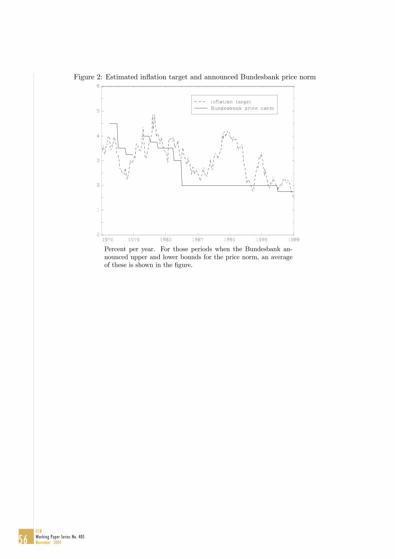
Figure 2: Estimated inflation target and announced Bundesbank price norm
Percent per year. For those periods when the Bundesbank an-nounced upper and lower bounds for the price norm, an averageof these is shown in the figure.
56ECBWorking Paper Series No. 405November 2004

Figure 3: Impulse responses from inflation target shock
All responses are expressed in percentage terms. The inflationand short rate responses are expressed in annual terms. Dottedlines are 95% confidence bands. The inflation target was shockedby one standard deviation (around 0.2% p.a.).
57ECB
Working Paper Series No. 405November 2004
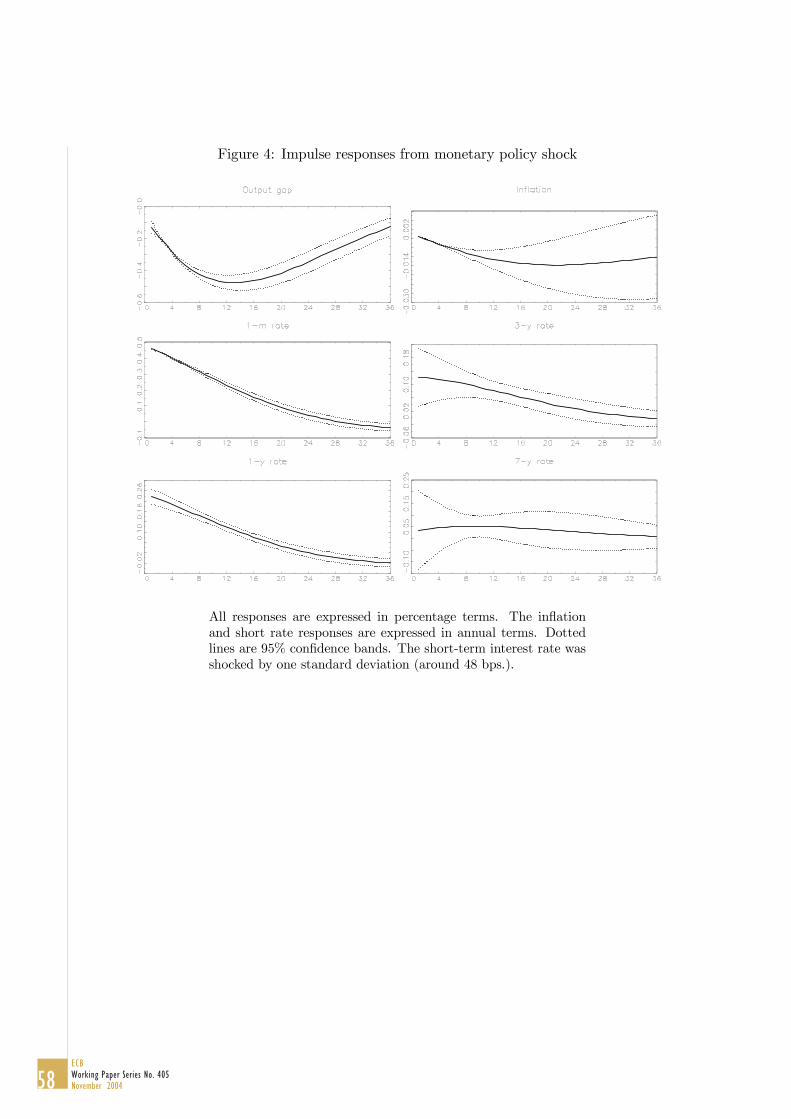
Figure 4: Impulse responses from monetary policy shock
All responses are expressed in percentage terms. The inflationand short rate responses are expressed in annual terms. Dottedlines are 95% confidence bands. The short-term interest rate wasshocked by one standard deviation (around 48 bps.).
58ECBWorking Paper Series No. 405November 2004

Figure 5: Impulse responses from inflation shock
All responses are expressed in percentage terms. The inflation andshort rate responses are expressed in annual terms. Dotted linesare 95% confidence bands. Inflation was shocked by one standarddeviation (around 0.26% p.a.).
59ECB
Working Paper Series No. 405November 2004

Figure 6: Impulse responses from output shock
All responses are expressed in percentage terms. The inflationand short rate responses are expressed in annual terms. Dottedlines are 95% confidence bands. The output gap was shocked byone standard deviation (around 1.2%).
60ECBWorking Paper Series No. 405November 2004
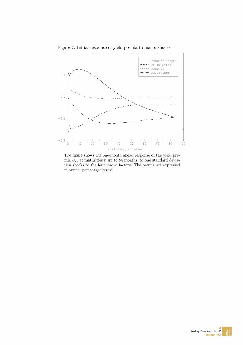
Figure 7: Initial response of yield premia to macro shocks
The figure shows the one-month ahead response of the yield pre-mia ��, at maturities � up to 84 months, to one standard devia-tion shocks to the four macro factors. The premia are expressedin annual percentage terms.
61ECB
Working Paper Series No. 405November 2004

Figure 8: Estimated yield premia and components of premia
The solid lines are the estimated (de-meaned) yield premiums �� during the sample period,for maturities � = 12 and 84 months, expressed in annual percentage terms. The dashedlines show the portions of the premia that are due to selected macro factors or combinationsof such factors.
62ECBWorking Paper Series No. 405November 2004

Figure 9: Model-implied CS projection coefficients: ”LPY (i)”
Empirical estimates of the CS long-rate coefficients ��in ��−1
�+1 −���= �
�(��
�− ��) � (�− 1), plus corresponding model-implied cof-
ficient values. The "population" coefficients are the theoreticalvalues based on our estimates; the MC coefficients are the meanestimates from 1000 series of the same size as the sample, simu-lated from our model. The bands around the MC mean estimatesare 5% confidence bands.
63ECB
Working Paper Series No. 405November 2004

Figure 10: Model-implied risk-premium adjusted CS coefficients: ”LPY (ii)”
The figure shows the estimates of the Campbell and Shiller(1991) long-rate coefficients �
�in the regression ��−1
�+1 − ���=
��(��
�− ��) � (�− 1) for our sample, along with the correspond-
ing risk-premium adjusted model-implied cofficient values basedon our parameter estimates.
64ECBWorking Paper Series No. 405November 2004

65ECB
Working Paper Series No. 405November 2004
European Central Bank working paper series
For a complete list of Working Papers published by the ECB, please visit the ECB’s website(http://www.ecb.int)
380 “Optimal monetary policy under discretion with a zero bound on nominal interest rates”by K. Adam and R. M. Billi, August 2004.
381 “Fiscal rules and sustainability of public finances in an endogenous growth model”by B. Annicchiarico and N. Giammarioli, August 2004.
382 “Longer-term effects of monetary growth on real and nominal variables, major industrialcountries, 1880-2001” by A. A. Haug and W. G. Dewald, August 2004.
383 “Explicit inflation objectives and macroeconomic outcomes” by A. T. Levin, F. M. Natalucciand J. M. Piger, August 2004.
384 “Price rigidity. Evidence from the French CPI micro-data” by L. Baudry, H. Le Bihan,P. Sevestre and S. Tarrieu, August 2004.
385 “Euro area sovereign yield dynamics: the role of order imbalance” by A. J. Menkveld,Y. C. Cheung and F. de Jong, August 2004.
386 “Intergenerational altruism and neoclassical growth models” by P. Michel, E. Thibaultand J.-P. Vidal, August 2004.
387 “Horizontal and vertical integration in securities trading and settlement” by J. Tapkingand J. Yang, August 2004.
388 “Euro area inflation differentials” by I. Angeloni and M. Ehrmann, September 2004.
389 “Forecasting with a Bayesian DSGE model: an application to the euro area” by F. Smetsand R. Wouters, September 2004.
390 “Financial markets’ behavior around episodes of large changes in the fiscal stance” byS. Ardagna, September 2004.
391 “Comparing shocks and frictions in US and euro area business cycles: a Bayesian DSGEapproach” by F. Smets and R. Wouters, September 2004.
392 “The role of central bank capital revisited” by U. Bindseil, A. Manzanares and B. Weller,September 2004.
393 ”The determinants of the overnight interest rate in the euro area”by J. Moschitz, September 2004.
394 ”Liquidity, money creation and destruction, and the returns to banking”by Ricardo de O. Cavalcanti, A. Erosa and T. Temzelides, September 2004.
395 “Fiscal sustainability and public debt in an endogenous growth model”by J. Fernández-Huertas Moraga and J.-P. Vidal, October 2004.

66ECBWorking Paper Series No. 405November 2004
396 “The short-term impact of government budgets on prices: evidence from macroeconomicmodels” by J. Henry, P. Hernández de Cos and S. Momigliano, October 2004.
397 “Determinants of euro term structure of credit spreads” by A. Van Landschoot, October 2004.
398 “Mergers and acquisitions and bank performance in Europe: the role of strategic similarities”
399 “Sporadic manipulation in money markets with central bank standing facilities”by C. Ewerhart, N. Cassola, S. Ejerskov and N. Valla, October 2004.
400
401 “Foreign direct investment and international business cycle comovement” by W. J. Jansenand A. C. J. Stokman, October 2004.
402 “Forecasting euro area inflation using dynamic factor measures of underlying inflation”
403 “Financial market integration and loan competition: when is entry deregulation sociallybeneficial?” by L. Kaas, November 2004.
404 “An analysis of systemic risk in alternative securities settlement architectures”by G. Iori, November 2004.
405 “A joint econometric model of macroeconomic and term structure dynamics”by P. Hördahl, O. Tristani and D. Vestin, November 2004.
by G. Camba-M ndez and G. Kapetanios, November 2004.
J. Morgan and J. Valles, October 2004.“Cross-country differences in monetary policy transmission” by R.-P. Berben, A. Locarno,
by Y. Altunbas and D. Marqués Ibáñez, October 2004.
é

Recommended