THE COOPER UNION
ALBERT NERKEN SCHOOL OF ENGINEERING
A Generative Model for Digital Camera
Chemical Colorimetry
by
Jason Tam
A thesis submitted in partial fulfillment
of the requirements for the degree of
Master of Engineering
Tuesday 3rd May, 2016
Advised by: Dr. Sam M. Keene

THE COOPER UNION FOR THE ADVANCEMENT OF SCIENCE AND ART
ALBERT NERKEN SCHOOL OF ENGINEERING
This thesis was prepared under the direction of the Candidate’s Thesis Advisor and has
received approval. It was submitted to the Dean of the School of Engineering and the full
Faculty, and was approved as partial fulfillment of the requirements for the degree of Master
of Engineering.
Dr. Richard J. Stock - Tue 3rd May, 2016
Dean, School of Engineering
Prof. Sam M. Keene - Tue 3rd May, 2016
Candidate’s Thesis Advisor

Acknowledgements
First and foremost, I would like to thank my advisor, Professor Sam Keene. He told me to
go finish my thesis – and so I started working on my thesis.
I extend my thanks to Victoria Heinz and Revans Ragbir, who taught me basic high school
chemistry and helped me with work in the chemistry lab.
I thank my ex-employer, Pixie Scientific, for introducing me to the applications and struggles
of portable colorimetry – ultimately motivating this work.
And lastly, I thank the individuals who actually took the time to read through this work
and provide feedback for me to improve.
i

THE COOPER UNION
Abstract
Dr. Sam M. Keene
Albert Nerken School of Engineering
Master of Engineering
by Jason Tam
This thesis presents a generative model for camera RGB values given latent variables
that govern a material’s surface reflectance spectra. Specifically, the RGB values of a
bromothymol-blue based pH indicator strip as captured by a Nokia N900 camera, will be
investigated. The model consists of two main components: a model of the pH indicator’s
surface reflectance spectra with the pH of the dipped solution as its latent variable, and
a model of the camera imaging pipeline. The generative model is then used in a machine
learning application to predict the latent variable, pH, given image observations from a
camera. Additionally, the model provides a scheme for data augmentation. The generative
model performs competitively against other traditional regression techniques. When used
for data augmentation, the model improves the performance of other learning algorithms
trained on the same dataset. Therefore, when sufficient domain knowledge is present, sim-
ilar generative models to this one could be used to lessen the amount of data collection
required.
Contents
Declaration of Approval
Acknowledgements i
Abstract ii
List of Figures vi
List of Tables vii
Physical Constants viii
1 Introduction 1
1.1 Organization . . . . . . . . . . . . . . . . . . . . . . . . . . . . . . . . . . . 2
2 Background 3
2.1 Light and Atomic Models . . . . . . . . . . . . . . . . . . . . . . . . . . . . 3
2.2 Illumination . . . . . . . . . . . . . . . . . . . . . . . . . . . . . . . . . . . . 5
2.2.1 Incandescent . . . . . . . . . . . . . . . . . . . . . . . . . . . . . . . 5
2.2.2 Compact Fluorescent (CFL) . . . . . . . . . . . . . . . . . . . . . . . 6
2.2.3 Light Emitting Diode (LED) . . . . . . . . . . . . . . . . . . . . . . 6
3 Spectra Construction 8
3.1 Absorption Spectra of Bromothymol Blue . . . . . . . . . . . . . . . . . . . 8
3.1.1 Chemistry of Acid-Base Indicator Reactions . . . . . . . . . . . . . . 8
3.1.2 Approximate Absorption Spectra Model . . . . . . . . . . . . . . . . 9
3.2 Absorption to Reflectance . . . . . . . . . . . . . . . . . . . . . . . . . . . . 10
3.3 Surface Geometry . . . . . . . . . . . . . . . . . . . . . . . . . . . . . . . . . 12
4 Imaging Pipeline 13
4.1 Optics . . . . . . . . . . . . . . . . . . . . . . . . . . . . . . . . . . . . . . . 13
4.2 Sensor . . . . . . . . . . . . . . . . . . . . . . . . . . . . . . . . . . . . . . . 14
4.2.1 Infrared (IR) Filter . . . . . . . . . . . . . . . . . . . . . . . . . . . . 14
4.2.2 Microlens Array . . . . . . . . . . . . . . . . . . . . . . . . . . . . . 15
iii

Contents iv
4.2.3 Color Filter Array (CFA) . . . . . . . . . . . . . . . . . . . . . . . . 16
4.2.4 CCD and CMOS Sensors . . . . . . . . . . . . . . . . . . . . . . . . 16
4.2.4.1 Charge-coupled Device (CCD) Sensors . . . . . . . . . . . 17
4.2.4.2 Complementary Metal-Oxide Semiconductor (CMOS) Sensors 18
4.2.5 Photosite Model . . . . . . . . . . . . . . . . . . . . . . . . . . . . . 18
4.2.6 Sensor Noise . . . . . . . . . . . . . . . . . . . . . . . . . . . . . . . 19
4.2.6.1 Photon Shot Noise and Photon Counts . . . . . . . . . . . 19
4.2.6.2 Dark Current and Thermal Noise . . . . . . . . . . . . . . 21
4.2.6.3 Reset Noise . . . . . . . . . . . . . . . . . . . . . . . . . . . 21
4.3 Post-processing . . . . . . . . . . . . . . . . . . . . . . . . . . . . . . . . . . 21
4.3.1 Demosaicing . . . . . . . . . . . . . . . . . . . . . . . . . . . . . . . 21
5 Sampling Methods 23
5.1 Monte Carlo Methods . . . . . . . . . . . . . . . . . . . . . . . . . . . . . . 23
5.1.1 Inverse Transform Sampling . . . . . . . . . . . . . . . . . . . . . . . 24
5.1.2 Rejection Sampling . . . . . . . . . . . . . . . . . . . . . . . . . . . . 25
5.2 Markov Chain Monte Carlo (MCMC) . . . . . . . . . . . . . . . . . . . . . 26
5.2.1 Markov Chains . . . . . . . . . . . . . . . . . . . . . . . . . . . . . . 27
5.2.2 Metropolis-Hastings . . . . . . . . . . . . . . . . . . . . . . . . . . . 28
5.2.3 Gibbs Sampling . . . . . . . . . . . . . . . . . . . . . . . . . . . . . . 30
5.2.4 Metropolis-within-Gibbs . . . . . . . . . . . . . . . . . . . . . . . . . 32
5.2.5 Thinning . . . . . . . . . . . . . . . . . . . . . . . . . . . . . . . . . 32
5.2.6 Burn-In . . . . . . . . . . . . . . . . . . . . . . . . . . . . . . . . . . 32
6 MCMC Colorimetry 34
6.1 Bayesian Network Model . . . . . . . . . . . . . . . . . . . . . . . . . . . . . 34
6.1.1 Surface Model . . . . . . . . . . . . . . . . . . . . . . . . . . . . . . 35
6.1.2 Illumination Model . . . . . . . . . . . . . . . . . . . . . . . . . . . . 36
6.1.3 Imaging Model . . . . . . . . . . . . . . . . . . . . . . . . . . . . . . 36
6.2 Fitting . . . . . . . . . . . . . . . . . . . . . . . . . . . . . . . . . . . . . . . 38
6.2.1 Analytical Solution . . . . . . . . . . . . . . . . . . . . . . . . . . . . 40
6.2.2 Fitting on Measured Spectra . . . . . . . . . . . . . . . . . . . . . . 40
6.2.3 Fitting on Observations . . . . . . . . . . . . . . . . . . . . . . . . . 41
6.3 Prediction . . . . . . . . . . . . . . . . . . . . . . . . . . . . . . . . . . . . . 41
6.3.1 Maximum A Posteriori (MAP) Estimation . . . . . . . . . . . . . . . 42
6.4 Data Augmentation . . . . . . . . . . . . . . . . . . . . . . . . . . . . . . . 42
7 Implementation & Experimental 44
7.1 Software Implementations . . . . . . . . . . . . . . . . . . . . . . . . . . . . 44
7.1.1 Imaging Pipeline . . . . . . . . . . . . . . . . . . . . . . . . . . . . . 44
7.1.2 Graph Model and MCMC . . . . . . . . . . . . . . . . . . . . . . . . 44
7.2 Data Collection . . . . . . . . . . . . . . . . . . . . . . . . . . . . . . . . . . 45
7.2.1 Imaging Device . . . . . . . . . . . . . . . . . . . . . . . . . . . . . . 45
7.2.2 Sample Preparation . . . . . . . . . . . . . . . . . . . . . . . . . . . 45
7.2.3 Solution Preparation . . . . . . . . . . . . . . . . . . . . . . . . . . . 46

Contents v
7.2.4 Illumination . . . . . . . . . . . . . . . . . . . . . . . . . . . . . . . . 46
7.2.5 Positional Setup . . . . . . . . . . . . . . . . . . . . . . . . . . . . . 47
7.3 Camera Calibration . . . . . . . . . . . . . . . . . . . . . . . . . . . . . . . 47
7.3.1 Linear Scaling . . . . . . . . . . . . . . . . . . . . . . . . . . . . . . 48
7.3.2 N-way Channel Interactions . . . . . . . . . . . . . . . . . . . . . . . 48
8 Results and Discussion 50
8.1 MAP Estimate Results . . . . . . . . . . . . . . . . . . . . . . . . . . . . . . 50
8.2 Data Augmentation Results . . . . . . . . . . . . . . . . . . . . . . . . . . . 52
8.3 Approximated Posterior . . . . . . . . . . . . . . . . . . . . . . . . . . . . . 53
9 Conclusion 55
9.1 Future Work . . . . . . . . . . . . . . . . . . . . . . . . . . . . . . . . . . . 55
A Experiment Preparation 57
A.1 pH Buffer Creation . . . . . . . . . . . . . . . . . . . . . . . . . . . . . . . . 57
A.1.1 Objective . . . . . . . . . . . . . . . . . . . . . . . . . . . . . . . . . 57
A.1.2 Procedure . . . . . . . . . . . . . . . . . . . . . . . . . . . . . . . . . 57
B Relevant Source Code 59
B.1 Bayesian Network Model . . . . . . . . . . . . . . . . . . . . . . . . . . . . . 59
B.2 Camera Model . . . . . . . . . . . . . . . . . . . . . . . . . . . . . . . . . . 65
C Performance Metrics 81
Bibliography 82

List of Figures
2.1 Depictions of the Bohr atom model via [1] . . . . . . . . . . . . . . . . . . . 4
4.1 Cross-sectional view of simplified pixel array via [2] . . . . . . . . . . . . . . 15
4.2 Depictions of the Bayer CFA via [3] . . . . . . . . . . . . . . . . . . . . . . 16
5.1 Step in Rejection sampling. In this case, x(i) is accepted because u < p(x(i))
Mq(x(i))
and falls in the accept region. (adapted from [4]) . . . . . . . . . . . . . . . 26
5.2 Graphical depiction of a sample Markov chain with transition matrix andinitial probability vector shown to the right . . . . . . . . . . . . . . . . . . 28
5.3 Example of Gibbs sampling in 2 dimensions via [5] . . . . . . . . . . . . . . 30
5.4 Example of a sequence of samples where one might burn in roughly 1000samples due to poor initialization. via [6] . . . . . . . . . . . . . . . . . . . 33
6.1 Full Bayesian network model including surface, illuminant, and imaging nodes.Round nodes represent stochastic nodes, and triangular nodes represent de-terministic nodes. . . . . . . . . . . . . . . . . . . . . . . . . . . . . . . . . . 37
6.2 Peak heights fitted with logistic functions. . . . . . . . . . . . . . . . . . . . 39
7.1 Spectral power distributions of the two illuminants used. . . . . . . . . . . . 46
7.2 Simulated and observed Macbeth ColorChecker arrangements with and with-out an estimated digital gain. 2-way channel interactions are used for thisparticular digital gain. . . . . . . . . . . . . . . . . . . . . . . . . . . . . . . 49
8.1 Hand-picked examples of some estimated posteriors via MCMC. 8.1a showsa well approximated posterior. 8.1b exemplifies an unfortunate case wherethe approximated posterior was overly confident in values very close to thetrue pH. . . . . . . . . . . . . . . . . . . . . . . . . . . . . . . . . . . . . . . 54
vi

List of Tables
6.1 List of nodes in the Bayesian network . . . . . . . . . . . . . . . . . . . . . 38
7.1 Nokia N900 camera specifications via [7] . . . . . . . . . . . . . . . . . . . . 45
8.1 Comparison of regression performances for various models trained on datafrom a single illuminant. Bold values denote the best performance for a givenevaluation metric and training illumination. . . . . . . . . . . . . . . . . . . 51
8.2 Regression performance for various models trained on data from a singleilluminant compared against models trained with augmented data. Metricslabeled with ’da’ denote the use of data augmentation. Bold values denotethe best performance for a given evaluation metric and training illumination. 52
8.3 Comparison of the approximated posterior with a uniform distribution overpH 6 to 8. Both the mean and median over all performances are providedfor the MCMC posterior. . . . . . . . . . . . . . . . . . . . . . . . . . . . . 54
A.1 Ratios of citric acid and sodium phosphate used to create gradation of pHbuffers. Taken from [8] . . . . . . . . . . . . . . . . . . . . . . . . . . . . . 58
vii

Physical Constants
Speed of Light c = 2.997 924 58× 108 [m/s]
Planck’s Constant h = 6.626 070 04× 10−34 [J · s]
Boltzmann’s Constant kB = 1.380 648 52× 10−23 [J/K]
viii
Chapter 1
Introduction
Color provides some of the most useful information in today’s world. The color of a banana
can help determine whether it is ripe. The color of sunlight is related to the time of day. And
the color perceived by different individuals can determine whether or not that individual is
color-blind.
Colorimetry, in the field of chemistry, refers to the use of color information to determine
concentrations of a given analyte within a solution. One of the most portable and practical
methods of colorimetry is the use of colorimetric test strips (a pH indicator test strip for
example [9]). These test strips contain a chemical indicator that changes colors when ex-
posed to various levels of analyte. The color of the strip, as observed by either machine or
human, is then compared to a reference to determine the approximate analyte level. The
portability and speed of these products have made them very attractive in point of care
health diagnostics. Since the logging, tracking, and communication of results is very impor-
tant in the world of health-care, many have been quick to merge smart-phone technology
into this field of test strip colorimetry [10][11][12]. The premises behind these works is to
utilize the smart-phone’s camera as the observer of the test strip’s color. Unfortunately,
the way these works handle disparate illumination sources is still quite inelegant – requiring
recalibration, in-frame references, or ignoring the problem all-together. Another solution
would be to collect vasts amounts of data to capture the variances introduced by different
1

Chapter 1 Introduction 2
illumination sources. However, data, and the collection of data, is expensive in labor and
time.
A commonality between these current methods ([10][11][12]) is that there is very little
consideration into how the data is generated – there is still much domain knowledge left
untouched. The goal of this thesis is to construct a generative model for colorimetry with
chemical indicator test strips and standard digital imaging. Additionally, the use cases of
the generative model from a machine learning perspective will be investigated.
1.1 Organization
As the goal is to construct a generative model involving color, it is necessary to cover some
background on why the notion of color exists in the first place. Chapter 2 discusses some
basic theory of light and atomic theory. This gives a foundation of why different materials
can have different colors and why the material may seem to have different colors under
different illuminants. Chapter 3 will then cover the surface spectra with respect to chemical
indicators. The observer of color in this context is a digital camera; as such, chapter 4 will
cover how digital cameras work and walk through the digital imaging pipeline.
The key point of a generative model is being able to simulate data. In particular, this
thesis relies on Monte Carlo methods to sample from the model. As is the case, chapter
5 will explore various Monte Carlo sampling methods. Chapter 6 will propose the novel
work of this thesis, describing the construction of the model itself along with its use cases.
The implementation of the model and experimentation follows in chapter 7. The results
of comparing predictions of the generative model against uninformed traditional regression
models are shown in chapter 8. Finally, some concluding remarks and discussion of future
considerations will take place in chapter 9.
Chapter 2
Background
2.1 Light and Atomic Models
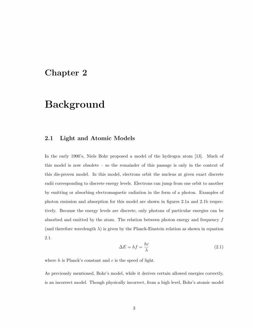
In the early 1900’s, Niels Bohr proposed a model of the hydrogen atom [13]. Much of
this model is now obsolete – so the remainder of this passage is only in the context of
this dis-proven model. In this model, electrons orbit the nucleus at given exact discrete
radii corresponding to discrete energy levels. Electrons can jump from one orbit to another
by emitting or absorbing electromagnetic radiation in the form of a photon. Examples of
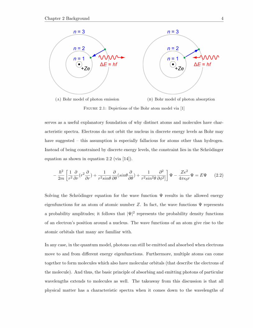
photon emission and absorption for this model are shown in figures 2.1a and 2.1b respec-
tively. Because the energy levels are discrete, only photons of particular energies can be
absorbed and emitted by the atom. The relation between photon energy and frequency f
(and therefore wavelength λ) is given by the Planck-Einstein relation as shown in equation
2.1.
∆E = hf =hc
λ(2.1)
where h is Planck’s constant and c is the speed of light.
As previously mentioned, Bohr’s model, while it derives certain allowed energies correctly,
is an incorrect model. Though physically incorrect, from a high level, Bohr’s atomic model
3
Chapter 2 Background 4
(a) Bohr model of photon emission (b) Bohr model of photon absorption
Figure 2.1: Depictions of the Bohr atom model via [1]
serves as a useful explanatory foundation of why distinct atoms and molecules have char-
acteristic spectra. Electrons do not orbit the nucleus in discrete energy levels as Bohr may
have suggested – this assumption is especially fallacious for atoms other than hydrogen.
Instead of being constrained by discrete energy levels, the constraint lies in the Schrodinger
equation as shown in equation 2.2 (via [14]).
− ~2
2m
[1
r2∂
∂r(r2
∂
∂r) +
1
r2sinθ
∂
∂θ(sinθ
∂
∂θ) +
1
r2sin2θ
∂2
∂φ2]
]Ψ− Ze2
4πε0rΨ = EΨ (2.2)
Solving the Schrodinger equation for the wave function Ψ results in the allowed energy
eigenfunctions for an atom of atomic number Z. In fact, the wave functions Ψ represents
a probability amplitudes; it follows that |Ψ|2 represents the probability density functions
of an electron’s position around a nucleus. The wave functions of an atom give rise to the
atomic orbitals that many are familiar with.
In any case, in the quantum model, photons can still be emitted and absorbed when electrons
move to and from different energy eigenfunctions. Furthermore, multiple atoms can come
together to form molecules which also have molecular orbitals (that describe the electrons of
the molecule). And thus, the basic principle of absorbing and emitting photons of particular
wavelengths extends to molecules as well. The takeaway from this discussion is that all
physical matter has a characteristic spectra when it comes down to the wavelengths of

Chapter 2 Background 5
photons it can emit or absorb. And this characteristic spectra is dependent on the orbitals
of the molecule or atom.
2.2 Illumination
One of the key components of an object’s apparent color is the scene’s illumination. As
hinted in section 2.1, the spectral power distribution (SPD) of an illuminant is dependent
on the molecular composition of the illumination source. In addition to natural sunlight,
there also exists many sources of artificial illuminants. The most common types of artificial
lighting include incandescent, compact fluorescent (CFL), and light emitting diode (LED).
The Commission internationale de l’eclairage (CIE) have standardized a set of specific
SPDs – these are known as the CIE standard illuminants. The following sections will
further discuss the aforementioned major sources of illumination and the corresponding
CIE standardization(s).
2.2.1 Incandescent
A light source caused by heating an object can be classified as an incandescent light source.
An incandescent illuminant commonly refers to a light bulb with a tungsten filament heated
by electrical current. As is the case, the CIE standard illuminant ’A’ represents an electrical
tungsten-filament light at a temperature of 2856K. And while many incandescent illumi-
nants are man-made, fires, hot coals, and even sunlight can be considered incandescent
illuminants. The D series of CIE standard illuminants refer to daylight illumination at
various times of the day.
Incandescent illuminants, as blackbody radiators, obey Planck’s radiation law in describing
the spectral energy given a temperature as shown below (reproduced via [13]):
E(λ, T ) =8πhc
λ5(exp (
hc
λkBT− 1))−1 (2.3)

Chapter 2 Background 6
where h is Planck’s constant, c is the speed of light, and kB is Boltzmann’s constant. It is
easily seen that equation 2.3 is highly differentiable – indicating that the SPDs of blackbody
radiators are very smooth. The SPD of a tungsten-filament incandescent source is shown
in figure 7.1a.
2.2.2 Compact Fluorescent (CFL)
The CIE F series of standard illuminants represent fluorescent lights of various color tem-
peratures. Compact fluorescent lights are literally just more compact versions of the larger
fluorescent tube lights. And as the name suggests, fluorescent lights work on the basis of
fluorescence. Fluorescence refers to the re-emission of light at different wavelengths than the
absorbed light. Substances that exhibit fluorescence are known as phosphors. The typical
construction of a CFL involves a gas filled tubed lined with phosphors. The source of light
in CFLs actually originates from the excitation of gas inside the bulb. From section 2.1, the
atomic structure of these gases restricts the wavelengths of light it can emit. This results in
the line spectra associated with gas excitation (think neon lights). Phosphors are used in
order to convert the emitted line spectra into more visually pleasing wavelengths. However,
phosphors only have a limited effect; thus, the SPDs of CFLs still contain very distinctive
peaks located at the wavelengths emitted via gas excitation. The SPD of a CFL source is
shown in figure 7.1b.
2.2.3 Light Emitting Diode (LED)
The newest of the three illuminants covered in this writing is the light emitting diode (LED).
The CIE has not (yet) created a standard for LEDs due to the technology being actively
improved on. LEDs work on the basis of electroluminescence – which refers to the emission
of light due to the application of an electric current or field. Recall from basic electronics, a
diode is constructed as a p-n junction. When electricity is applied, the holes in the p-type
semiconductor combine with the electrons in the n-type semiconductor. Energy is released

Chapter 2 Background 7
in the form of emitted photons in order for the recombination to occur. The SPD of LEDs
depends widely on the materials used for the p and n-type semiconductors.

Chapter 3
Spectra Construction
The subject being imaged is going to be a pH indicator test strip based on a bromothymol-
blue (BTB) dye. The rest of this section will describe how BTB works and how its reflectance
spectra can be modeled.
3.1 Absorption Spectra of Bromothymol Blue
3.1.1 Chemistry of Acid-Base Indicator Reactions
As with most chemical indicators, there exists a high-level, two-way reaction that is depen-
dent on some specific analyte; BTB is no different.
Acid-base indicators take on two states (symbolic representations given in parentheses 1):
a weak acid (HIn), or its conjugate base (In–). For BTB, the weak acid form has a peak
absorption of around 430nm, absorbing blue light and thus reflecting and appearing yellow.
On the other hand, its conjugate base form has a peak absorption of around 615nm, absorb-
ing yellow-orange light and thus reflecting and appearing blue. The transition from being a
weak acid to its conjugate base can be represented in the following two-way reaction (with
1these are generic symbols for indicators
8

Chapter 3 Spectra Construction 9
reference to [15]):
HInyellow
+ H2O −−→←−− H3O+ + In−
blue(3.1)
It follows that the average color of the indicator solution is dependent on the proportions
of acid and base present. The pH of the solution then has the following relation
pH = pKHIn + log[In−]
[HIn](3.2)
where pKa is the log acid dissociation constant – this is just an attribute of a given indicator.
BTB is a dye; as such, it follows Beer’s Law. Beer’s Law, or the Beer-Lambert Law, provides
the following relationship for transmittance T , and absorbance A:
T = 10−A (3.3)
A = εcs (3.4)
where ε is a material-dependent constant, c is the concentration of the absorbent species,
and s is the pathlength. The takeaway here is that the absorbance of a solution linearly
scales with concentration. This helps describe the behavior of mixing two dyes – as in
the case of an intermediate pH causing some concentration of HIn mixed with In–. Again,
in the context of BTB, this mixture would have some absorbance at around 430nm and
also at around 615nm causing a green appearance. The generalized expressions for the
transmittance and absorbance for n dye mixtures are given by (with reference to [13]):
Tmix(λ) =
n∏i=0
Ti(λ) (3.5)
Amix(λ) =
n∑i=0
Ai(λ) (3.6)
3.1.2 Approximate Absorption Spectra Model
Another way to think of these chemical indicators is to imagine two populations of molecules
that each have their own spectral absorbency characteristics. The analyte-level-dependent

Chapter 3 Spectra Construction 10
reaction simply moves members from one population to the other. The absorbency charac-
teristic per population can be modeled as a Gaussian distribution with mean and standard
deviation µi, σi, i ∈ 1, 2, where i represents the population. In the perspective of photons,
the distribution represents the probability of a photon of wavelength λ to be absorbed when
incident on the chemical indicator. On a macroscopic level, the spectral absorbency charac-
teristic of the indicator as a whole is then modeled as a one-dimensional Gaussian mixture
model (GMM) with mixture weights h.
The last variable to introduce into this model is the analyte level itself - in this case, the
pH. As discussed previously, the ratio of populations of the chemical indicator is designed
to be dependent of the analyte level. In the model, this translates to the mixture weights,
h, being a function of the analyte level. Empirically, it is also observed that the other GMM
parameters can be slightly dependent on the analyte level. Symbolically, the approximate
model can be represented as the following:
A(pH) ∝2∑i=1
hiN (µi, σi)
pH 7→ hi
pH 7→ µi
pH 7→ σi
(3.7)
3.2 Absorption to Reflectance
Chemical indicator solutions are mostly characterized by their absorption spectra. However,
in terms of imaging, it is the reflectance spectra that is desired. Recall Beer’s Law (equation
3.3), where absorbance was first mentioned. Reworking the terms of Beer’s law yields the
following definition of absorbance A:
A = log10(I0I
) (3.8)

Chapter 3 Spectra Construction 11
where I0 is the incident intensity of light, and I is the transmitted intensity of light. In
other words, for a translucent solution, incident light of initial intensity I0 passes through
the solution; some light gets absorbed and then light of intensity I is observed at the exiting
end of the solution. Note that for an absorption spectra, this measure is on a per-wavelength
basis.
Now consider the surface of an indicator test strip. The test strip is more or less a strip
of paper impregnated with an indicator solution (usually with some sort of mordant). The
simplifying assumption of a spectrally flat reflectance spectra can be made for the paper.
Even so, the reflectivity of paper cannot be perfect. Let the albedo, represented as α, of the
paper describe the ratio of reflected light to incident light. And let R represent the light
reflected from the indicator-impregnated strip of paper. From the perspective of the paper
itself, the intensity of transmitted light, I in equation 3.8, is treated as the intensity of light
incident on the paper. Putting this all together yields the following expression for R:
R ≈ αI =αI010A
(3.9)
where I0 can be taken as equal to 1 if the absorption spectra is normalized. This gives the
desired approximated transformation from absorption spectra into reflectance spectra.
Another assumption that has been sneaked in is the assumption of perfect impregnation.
In reality, when an indicator strip is dipped in a solution, extra dye will likely leak into the
solution that sits on top of the paper. Recall from Beer’s Law (equation 3.3) that additional
dye on top of the paper would have a finite pathlength; and thus, would attenuate both
incident and reflected light. There is a lot more that could be said about the actual optics
of scattering in the paper itself; however, the approximation mentioned beforehand is quite
sufficient.

Chapter 3 Spectra Construction 12
3.3 Surface Geometry
Finally, the geometry of the test strip surface must be considered on a microscopic level.
For microscopically smooth surfaces, surfaces tend to appear glossy and glare can be seen.
This occurs when the angle of incidence is equal to the angle of reflection and is known as
specular reflection. When the angles are not equal, it results in diffuse reflection. Note that
both of these types of reflections have not even had a chance to penetrate the surface and
interact with the dye. As is the case, the color and spectral profile of these reflections is
the same as the incident light. In total, an observer will witness a combination of specular
reflectance and the light reflected from the subsurface (light reflected from the dyed paper).
Sometimes the assumption of a perfect diffuse surface is made; this is called a Lambertian
surface. In this case, the surface uniformly reflects in all possible angles of reflection. This
still yields a small component of specular reflection. But since the component is so small,
a further simplifying assumption can then be made to just ignore specular reflection all-
together.

Chapter 4
Imaging Pipeline
To synthesize data, we simulate the imaging pipeline of a standard digital camera. The
following sections will describe a digital imaging pipeline where light enters the camera and
numerical measures are output. Note that these discussions will be tailored towards the
processing of color information rather than spatial information.
4.1 Optics
The purpose of the optics in a digital camera is to redirect light from the desired scene
to the area of the sensor. First, some terminology needs to be introduced. The energy
emanating from the scene incident at the optical entrance of the camera is known as the
scene radiance and has units[
Wm2·sterad
]. The desired output of the optics module and light
incident at the sensor is known as the image irradiance which has units of [ Wm2 ]. A simple
model for the conversion from radiance to irradiance is through the camera equation. The
camera equation is shown in equation 4.1 (via [16]).
Iimage(x, y, λ) ≈ πT (λ)
4(f/#)2Lscene
( xm,y
m, λ)
(4.1)
13

Chapter 4 Imaging Pipeline 14
where Iimage is the irradiance at the sensor, Lscene is the scene radiance, T (λ) is the lens
transmissivity, f/# is the f-number of the lens, and m is the lens magnification.
A full discussion of an imaging system’s optical system is beyond the scope of this thesis.
There are only a limited number of ways in which the optics of a camera can affect the color
of a subject. Firstly, note that T (λ) is the sole contributor to the dependence of Iimage on λ.
The lens transmissivity determines how much of each wavelength the lens will pass through;
the rest of the energy is either absorbed or reflected back. Given high quality glass, the lens
transmissivity is close to 1 for all visible wavelengths. As is the case, lens transmissivity
can usually be assumed to equal 1 for most calculations [17].
Another way optics can have an effect on color is through aberrations. This is especially
the case in chromatic aberrations which are caused by a material’s index of refraction being
dependent on wavelength. This however, mainly only affects the edges of a given shape. As
is the case, aberrations are justifiably ignored in the simplified camera equation.
4.2 Sensor
The purpose of the imaging sensor is to spatially quantify photon fluxes emitted from a
scene. The following subsections are ordered following the path of irradiance. The last
subsection will discuss the some sources of noise associated with imaging sensors.
4.2.1 Infrared (IR) Filter
For illuminants such as incandescent bulbs and sunlight, there exists spectral power in the
infrared region (wavelengths from 700nm to 1mm). When these illuminants are combined
with materials, such as some foliage, which reflect the IR spectra, it is possible for imaging
sensors to witness large radiant fluxes of IR light. Even in the case of trace IR light, images
can seem off-colored when presented to a human. While the human visible spectrum is only
sensitive to wavelengths of 390nm to 700nm [18], the imaging sensor alone is sensitive to
IR light. Thus, many sensors include an IR filter at the very top / surface of the sensor.

Chapter 4 Imaging Pipeline 15
pixel
On-Chip Microlens Array
On-Chip Color Filter Array
Dielectric Material
Light Shield
n+ n+ n+ n+
P Photodiode
Substrate
Figure 4.1: Cross-sectional view of simplified pixel array via [2]
4.2.2 Microlens Array
Within the sensor, there is an additional piece of optics known as a microlens array. The
microlens array can be seen on the top of Figure 4.1. Each pixel1 has a tunnel-like geometry,
and in newer CMOS sensors with many layers, this tunnel can be quite deep [16]. So the
microlens has the important job of guiding the photons incident at the surface of the pixel
to the photodiode at the end without being lost at the tunnel walls.
Since the photodiodes are typically smaller than the aperture of the pixel itself, the microlens
preserves the effective pixel aperture. A closely related term is the fill factor (FF) of a pixel.
A pixel’s FF, as defined in Equation 4.2, is the ratio of a pixel’s photosensitive area to the
total pixel area.
FF = Apd/Apx (4.2)
1pixels are also sometimes referred to as photosites

Chapter 4 Imaging Pipeline 16
(a) An example of a Bayer pattern CFA over asensor array
Incoming light
Filter layer
Sensor array
Resulting pattern
(b) Tracing incoming light through the R, G,and B filters of the CFA
Figure 4.2: Depictions of the Bayer CFA via [3]
4.2.3 Color Filter Array (CFA)
In order to mimic the three (long, medium, and short) cones of the human visual system,
camera sensors typically make use of three color filters. It is challenging for sensor designers
and manufacturers to incorporate all three color filters into a single pixel (Foveon X3 sensors
do this [19]). As a result, most sensors spatially distribute the three color filters over all
pixels in what is called a Color Filter Array (CFA). The actual distribution and pattern of
the CFA can exhibit different pros and cons. Currently, the most popular CFA is the Bayer
filter pattern [20]. The basic 2x2 pixel tile of the Bayer pattern consists of 1 red, 2 green,
and 1 blue color filters arranged such that the green filters are on diagonal opposites. The
reason for having two green filters is to, again, mimic the human visual system which is
more sensitive to spectral green [13].
4.2.4 CCD and CMOS Sensors
At the time of writing, the two predominant image sensor technologies are charge-coupled
devices (CCD) and complementary metal-oxide semiconductor (CMOS) sensors. More
specifically, these two technologies are responsible for the main photodetection and con-
version portion of the image sensor.
While differing in name, CCD and CMOS sensor technologies still share many common-
alities. Both technologies utilize photodetectors for photon to electron conversion. These
Chapter 4 Imaging Pipeline 17
photodetectors, usually photodiodes or photogates, have a specification known as full-well
capacity 2, which defines the maximum charge accumulation during an exposure before
saturation. Full-well capacity is often measured in [# electrons]. The photodiodes, yield an
electrical current at each pixel which must be converted to a voltage with a measure known
as conversion gain [Volts/electron]. Additionally, a secondary analog gain, also measured
in [Volts/electron], can be applied and is often used as the digital counterpart to ISO sen-
sitivity in analog film. Having a unitary analog gain can be seen as imaging in the sensors
native ISO. The voltage is then quantized to a digital value using an analog-to-digital (A/D)
converter.
The following sections will discuss the differences between the two technologies in terms of
implementation and the resulting pros / cons.
4.2.4.1 Charge-coupled Device (CCD) Sensors
A distinctive feature of the CCD sensor technology is its method of reading out pixel values.
In CCDs, there is typically only a single pipe for pixel readout. Thus, CCDs are mostly
bottlenecked by their serial readout procedure (one pixel at a time).
In the simplest CCD architecture, named full-frame, the entire area of the sensor is dedicated
to the photodetectors. Thus, the fill factor of full-frame CCDs is very high - nearing or
reaching 100%. However, the full-frame architecture by itself in incapable of having an
electronic shutter, and so a mechanical shutter must be used.
The frame-transfer architecture, is an extension to full-frame which includes an opaque
storage area. An electronic shutter is used to transfer the entire frame of the photodetectors
into the storage area after integrating over the desired exposure time. Since the opaque
storage area is on another dedicated area of the sensor, the equivalent sensor is twice as
large and thus twice as expensive. The upside is that the fill factor of the frame-transfer
architecture is just as high as the full-frame architecture.
2Full-well capacity is also known as well-capacity and saturation charge, and is closely related to an imagesensor’s dynamic range
Chapter 4 Imaging Pipeline 18
The last major CCD architecture, called inter-line, also contains a storage mechanism but
not in a dedicated manner. Instead, the storage area is distributed in lines alternating with
the photodetectors. The compromise is that the photosite area is roughly halved resulting
in a 50% fill factor. However, with the use of a microlens array, as discussed in section 4.2.2,
the fill factor can be as high as 90%.
4.2.4.2 Complementary Metal-Oxide Semiconductor (CMOS) Sensors
The biggest difference with CMOS sensors when compared to CCD sensors is the change
from a primarily serial readout pipeline to a parallel one. CMOS technology allows much of
the readout logic and circuitry to be combined into the pixel itself. Thus, it is possible for
photon-to-electron conversion, electron-to-voltage conversion, and even A/D conversion to
all take place on a per-pixel basis. Due to the added responsibilities of each pixel in CMOS
sensors, they are referred to as active pixels - making up an active pixel sensor (APS) 3.
In the case that each pixel has its own A/D converter, the sensor is called a digital pixel
sensor - as each pixel now outputs a digital value.
In addition to bypassing the bottlenecks of a serial pipeline, having digital pixels allows
selective pixel processing such as digital zooming / cropping, and efficient region-based
metering.
However, the downside to integrating all this extra functionality in each pixel is that it
requires physical space. That is, the fill factor of CMOS sensors suffers when compared to
CCD sensors. Here again, is where the microlenses of section 4.2.2 comes in handy.
4.2.5 Photosite Model
Since the end goal will require simulation of a sensor, it is necessary to model the photosite.
Recall that a photosite collects photon-generated electrons during the exposure time ∆t.
The spectral irradiance incident at the photosite, E(λ), has already passed through the
3Early CMOS sensors also exist with just 1 amplifier transistor - they were called Passive pixel sensors(PPS)
Chapter 4 Imaging Pipeline 19
optics of the camera, the IR filter, the microlens, and the color filter associated with the
pixel. Let ck(λ) represent the ratio of electrons generated to incident light energy on a per-
wavelength basis – this is known as quantum efficiency. Let the photosite have dimensions
u× v. The total amount of charge accumulated in a photosite at pixel index (x, y) during
an exposure can then be given as (via [13]):
Q(x, y) = ∆t
∫λ
∫ x+u
x
∫ y+v
yE(x, y, λ)Sr(x, y)ck(λ)dxdydλ (4.3)
Sr is the spatial response of the pixel, which can be modeled as just a constant.
As mentioned in section 4.2.4, the charge collected at the photosite, Q, is then converted
into a voltage via an analog gain. This is simply a linear scaling of the charge by gain g as
shown below.
V = Q · g (4.4)
4.2.6 Sensor Noise
As previously mentioned, imaging sensors, both CCD and CMOS, are subject to noise. The
following sections discuss various sources and types of noise.
4.2.6.1 Photon Shot Noise and Photon Counts
Due to the particle nature of light, the arrival of photons at the imaging sensor’s photode-
tectors is discrete and exhibits a Poisson distribution. Therefore, photon shot noise is also
commonly referred to as Poisson noise.
A Poisson distribution is completely characterized by a single parameter λ. Unfortunately,
we have already reserved the λ symbol in representing wavelength. As is the case, let µ be the
parameter that describes Poisson distributions from here on. Given a Poisson distribution
with parameter µ, the distribution will have a mean of µ, and standard deviation of√µ.

Chapter 4 Imaging Pipeline 20
In order to incorporate photon shot noise into a mathematical model, the irradiance needs
to be converted into a photon count. The energy associated with a photon of a given
wavelength is determined by the following relation (recall the Planck relation from equation
2.1):
Ephoton(λ) =h · cλ
(4.5)
where h is Planck’s constant, and c is the speed of light. Recall from section 4.1 that
irradiance, a measure of energy flux per unit area, has units [ Wm2 ]. Dividing the energy flux
by the energy of a photon yields photon flux as shown below
Φphoton(λ) =I(λ)
Ephoton=I(λ) · λh · c
(4.6)
where I(λ) is the irradiance of a particular wavelength. Photon flux has units [#photonsm2·s ];
and so integrating over the size of the photosite and over the exposure time (as in equation
4.3) would yield units of [#photons]. The number of photons resulting from integrating
over space and time is actually the expected average number of arriving photons. And so,
a value drawn from a Poisson distribution with parameter µ set to the average number of
photons will be the actual number of photons arriving at the photosite.
The signal-to-noise ratio (SNR) 4 with respect to just shot noise is shown in equation 4.7.
SNshotR =µ√µ
=õ (4.7)
From this, it follows that photon shot noise is less of a problem when the number of photons
collected is high. This can be achieved for a given scene by increasing the aperture or
increasing the exposure time. Though, precaution should still be taken to not overexpose
and saturate beyond the full-well capacity of the photodetector. Given sufficient light,
photon shot noise will be the predominate source of noise in the output signal. Thus, the
following discussions of noise sources will not be viewed as in-depth as above.
4SNR in imaging is defined as the ratio of the signal mean to the standard deviation of the noise. Thisis contrary to the primary definition of signal power over noise power.

Chapter 4 Imaging Pipeline 21
4.2.6.2 Dark Current and Thermal Noise
Even when the photodetector is not subject to any illumination, it is still possible for a
small current to exist through random electron and electron-hole generation. The small
amount of current that is present even when the sensor is in the dark is called dark current.
Because dark current arises from the thermal energy naturally present in the sensor, it is
also commonly referred to as thermal noise.
The arrival of electrons contributing to dark current is random and also exhibits a Poisson
distribution like the photon shot noise discussed in section 4.2.6.1. As such, component of
dark current present in the final signal is called dark current shot noise.
Bear in mind that dark current shot noise is independent of the number of photons and
number of electrons generated from photons. However, longer exposure times, where the
sensor heats up from being active, can lead to an undesirable amount of thermal noise.
Thus, it is even common for some scientific-grade cameras to include cooling units for long
exposure shots.
4.2.6.3 Reset Noise
Every time a new image is taken, the existing electrons of a pixel needs to be reset. The
process of resetting each pixel is however, imperfect. This is especially true in high frame-
rate video where there might not be enough time between frames to fully reset. In any case,
the residual in a pixel’s potential well lead to a source of noise known as reset noise.
4.3 Post-processing
4.3.1 Demosaicing
Recall from section 4.2.3, by design, the CFA only contains one color channel of information.
In order to reconstruct the color image while preserving resolution, the other two missing

Chapter 4 Imaging Pipeline 22
color channels must be interpolated at each pixel given the neighboring pixels.
One of the simplest methods of interpolation is bilinear interpolation. Bilinear interpolation
is also realizable with convolution kernels making it suitable for efficient computation.
The following are the kernels used for interpolation specifically for a Bayer pattern CFA.
fR = fB =
14
12
14
12 1 1
2
14
12
14
fG =
0 1
4 0
14 1 1
4
0 14 0
Another way to interpret this is: each interpolated value is equal to the average of the pixels
present in its neighborhood of 8 connectivity. This becomes apparent when the 3x3 kernel
is overlaid on a 3x3 block of the corresponding filter’s resulting pattern from Figure 4.2b.

Chapter 5
Sampling Methods
5.1 Monte Carlo Methods
Broadly speaking, Monte Carlo methods refer to computational simulations making use of
random sampling in order to obtain approximate results. The history of Monte Carlo takes
seed when Enrico Fermi invents the FERMIAC, an analog (mechanical) computer, to help
calculate neutron diffusion. Later in the 1940’s, Stan Ulam, John & Klari Von Neumann,
and Nick Metropolis design Monte Carlo controls into ENIAC (the first electronic turing-
complete computer) for research in physics [4]. Metropolis suggests to give the statistical
method the code name “Monte Carlo” in reference to the Monte Carlo Casino where Ulam’s
borrowed money from relatives to gamble[21].
Consider this example from [5], where the problem is solving for the expectation of some
function f(x):
E[f(x)] =
∫f(x)p(x)dz (5.1)
A Monte Carlo approach to this problem would be to approximate the expectation using:
f =1
L
L∑l=1
f(x(l)) (5.2)
23

Chapter 5 Sampling Methods 24
where L independent samples are drawn from the distribution p(x). Note that x can be
multidimensional and the accuracy of f is independent of x’s dimensionality. The problem
is now drawing independent samples from p(x) assuming a computer with adequate uniform
random number generation is at disposal.
5.1.1 Inverse Transform Sampling
It is already assumed that computers have the ability to sample uniformly distributed
random numbers (u ∼ U is given). But it does not take much more effort to sample
from other simple distributions. That is, perhaps a function f can be found such that the
distribution of y = f(u ∼ U(0,1)) matches a simple desired distribution. For such a function
f , y will be distributed as follows:
p(y) = p(u)
∣∣∣∣dudy∣∣∣∣ =
∣∣∣∣dudy∣∣∣∣ (5.3)
where p(u) = 1 since p(u) is the uniform distribution from 0 to 1. Integrating equation 5.3
over y yields:
u = F (y) ≡∫ y
−∞p(y)dy (5.4)
Equation 5.4 just so happens to be the cumulative distribution function (CDF) for the
distribution p(y). The CDF is often symbolically stylized as FX(x) = P (X ≤ x). Solving
for y obtains the following:
y = F−1(u) (5.5)
Hence, uniformly distributed random numbers can be transformed to fit a desired a distri-
bution by applying the inverse CDF of said desired distribution. However, calculating the
inverse of a distribution’s indefinite integral may not always be feasible or even possible.

Chapter 5 Sampling Methods 25
5.1.2 Rejection Sampling
Consider a complicated distribution p(x) that is difficult to sample from directly. However,
assume that p(x) can be evaluated for any given x up to a normalization constant. Now
suppose there is a simple distribution q(x) called the proposal distribution; this is something
that is perhaps simple enough to be sampled using the inverse transform sampling technique
of section 5.1.1. Now let M be a scaling constant such that Mq(x) ≥ p(x). The general idea
of rejection sampling is to repeatedly draw from the proposal distribution and then accept
or reject 1 the sample based on a simple acceptance criterion. The acceptance criterion for
a given sample x(i) is if a uniformly random point in the range [0,Mq(x(i))] is less than p(x)
(which can be evaluated by assumption). Algorithm 1 enumerates these steps and figure
5.1 depicts a sampling step in which the candidate sample is accepted.
Algorithm 1 Rejection Sampling Algorithm adapted from [4]
1: procedure Rejection sample(p, q,M)
2: i← 0
3: while i 6= N do . N is the total # of steps to sample
4: u ∼ U(0,1)
5: x(i) ∼ q(x) . Draw candidate state given current state
6: if u < p(x(i))
Mq(x(i))then . Acceptance criterion
7: i← i+ 1 . Accept sample x(i)
8: else
9: pass . Reject sample x(i)
10: end if
11: end while
12: return x
13: end procedure
Rejection sampling, as a simple method, comes with a crippling limitation. That is, some-
times, especially with high-dimensional spaces, a very large scaling factor M must be used in
1hence, rejection sampling is also known as the accept-reject algorithm

Chapter 5 Sampling Methods 26
Mq(x(i))
Accept Region Reject Region
p(x(i))
uMq(x(i))
x(i) ∼ q(x) x
Figure 5.1: Step in Rejection sampling.
In this case, x(i) is accepted because u < p(x(i))Mq(x(i))
and falls in the accept region. (adapted
from [4])
order to have the proposal distribution envelope p(x) (to meet the condition Mq(x) ≥ p(x))
over the domain of x. Consider the probability that a sample is accepted:
P (acceptance) =
∫(p(x(i))
Mq(x(i)))q(x)dx
=1
M
∫p(x)dx
=1
M
(5.6)
So when M is large, the probability of acceptance is low, Thus, rejection sampling is not
very practical in very high dimensions.
A method of improving rejection sampling is to make it adaptive. That is, the enveloping
proposal distribution q(x) can be constructed adaptively per iteration according to the mea-
sured values of the desired distribution p(x). While this can speed things up by increasing
the acceptance probability, it can also fail terribly for complex shaped distributions.
5.2 Markov Chain Monte Carlo (MCMC)
Markov Chain Monte Carlo (MCMC), as the name implies, refers to Monte Carlo methods
which employ Markov chains for sampling. Like the basic Monte Carlo methods discussed in
Chapter 5 Sampling Methods 27
section 5.1, MCMC is used under the assumption that samples cannot be drawn from p(x)
directly; however, p(x) can be evaluated for a given sample up to a normalizing constant.
First, an overview of Markov chains will be given. Then the use of Markov chains in
sampling algorithms will be explored.
5.2.1 Markov Chains
A stochastic process has the Markov property if it is memoryless – that is, the future of
the process is only dependent upon the current state and independent of the past. In
general, the Markov property can be of order n in which the next iteration depends on the
n previous iterations. But for the scope of this text, only first-order Markov chains will be
considered (assume first-order from now on). In symbolic form, the stochastic process x(i)
is a first-order Markov chain if the following holds true
p(x(i+1)|x(1), . . . , x(i)) = p(x(i+1)|x(i)) (5.7)
A Markov chain can be fully specified given an initial state probability vector, µ(x(1)), and
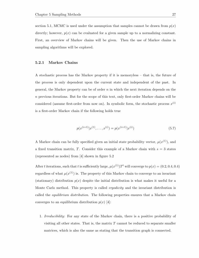
a fixed transition matrix, T . Consider this example of a Markov chain with s = 3 states
(represented as nodes) from [4] shown in figure 5.2
After t iterations, such that t is sufficiently large, µ(x(1))T t will converge to p(x) = (0.2, 0.4, 0.4)
regardless of what µ(x(1)) is. The property of this Markov chain to converge to an invariant
(stationary) distribution p(x) despite the initial distribution is what makes it useful for a
Monte Carlo method. This property is called ergodicity and the invariant distribution is
called the equilibrium distribution. The following properties ensures that a Markov chain
converges to an equilibrium distribution p(x) [4]:
1. Irreducibility : For any state of the Markov chain, there is a positive probability of
visiting all other states. That is, the matrix T cannot be reduced to separate smaller
matrices, which is also the same as stating that the transition graph is connected.

Chapter 5 Sampling Methods 28
1 0.9
0.4
0.6
0.1
x2
x1 x3
Figure 5.2: Graphical depiction of asample Markov chain with transition ma-trix and initial probability vector shown
to the right
T =
0 1 00 0.1 0.9
0.6 0.4 0
µ(x(1)) = (0.5, 0.2, 0.3)
2. Aperiodicity : The chain should not get trapped in cycles.
Alternatively, a sufficient (but not necessary) condition is
p(x(i))T (x(i−1)|x(i)) = p(x(i−1))T (x(i)|x(i−1)) (5.8)
or equivalently, after summing both sides over x(i−1),
p(x(i)) =∑x(i−1)
p(x(i−1))T (x(i)|x(i−1)) (5.9)
This condition is know as detail balance, and a Markov chain that satisfies the condition is
said to be reversible. When designing an MCMC sampler, it is important consider these
conditions and properties in constructing ergodic Markov chains.
5.2.2 Metropolis-Hastings
One of the most popular MCMC methods (and the foundation for most others) is the
Metropolis-Hastings (MH) algorithm. The MH sampling algorithm traverses through the
space of the desired posterior distribution, p, in a fashion such that it spends the most time

Chapter 5 Sampling Methods 29
in areas of high probability. At step i, given the current position x(i), the MH sampler will
look for a new position candidate x? based on a proposal distribution, q. The candidate
will be accepted with probability
A(x(i), x?) = min
{1,p(x?)
p(x(i))
q(x(i)|x?)q(x?|x(i))
}(5.10)
The motivation for having a stochastic rather than deterministic acceptance criterion is to
avoid having the sampler get stuck in any particular local maxima. That is, the sampler is
likely to stay near a modal peak, but there is always a non-zero chance for it to go out and
explore modes that might have been missed. Pseudo-code for the MH algorithm is shown
in algorithm 2.
Algorithm 2 Metropolis-Hastings algorithm (reproduced from [4])
1: procedure MH sample(p, q)
2: x0 ← Initial value
3: for i = 0 to N − 1 do . N is the total # of steps to sample
4: u ∼ U[0,1]
5: x? ∼ q(x?|x(i)) . Draw candidate state given current state
6: if u < A(x(i), x?) = min{
1, p(x?)
p(x(i))
q(x(i)|x?)q(x?|x(i))
}then . Acceptance criterion
7: x(i+1) ← x? . Move to candidate state
8: else
9: x(i+1) ← x(i) . Stay put
10: end if
11: end for
12: return x
13: end procedure
The original Metropolis algorithm just imposes the simplifying requirement that q must
be symmetric (q(x(i)|x?) = q(x?|x(i))); thus, A(x(i), x?) = min{
1, p(x?)
p(x(i))
}. The quotient,
q(x(i)|x?)q(x?|x(i)) , is thus, also known as the Hastings factor.

Chapter 5 Sampling Methods 30
x1
x2L
l
Figure 5.3: Example of Gibbs sampling in 2 dimensions via [5]
Like rejection sampling, the MH algorithm can also be made adaptive via its proposal
distribution q. If the proposal distribution is too narrow, the sampler will always have a
very high acceptance probability and will only take very small steps like a random walk.
On the other hand, if q is too wide, the rejection rate will be very high, and the sampler
will not move at all. In an adaptive scheme, the variance of the proposal distribution can
be tuned at each step to ensure a given acceptance probability is maintained.
5.2.3 Gibbs Sampling
Another popular MCMC algorithm is Gibbs sampling as described by Geman and Geman
[22]. Every step of the Gibbs sampler involves drawing a value for a given dimension
from the distribution conditioned on all other dimensions. This will be represented in the
following set-minus symbolic shorthand: x\k = {xj |j 6= k}. The pseudo-code for the Gibbs
sampler is shown in algorithm 3. The sampling steps 4-7 in the enumerated algorithm can
be done in any order. The important thing is that the sampler moves in one dimension at a
time within a given iteration. Note that for the jth dimension, the distribution, p(xj |x\j),
is conditioned on the (i+1)th iteration for dimensions before j and on the ith for dimensions
after j. An illustration of Gibbs sampling is shown in figure 5.3.

Chapter 5 Sampling Methods 31
Algorithm 3 Gibbs Sampling adapted from [4]
Let x\k = {xj |j 6= k}
1: procedure Gibbs sample(p)
2: i← 0
3: for i = 0 to N − 1 do . N is the total # of steps to sample
4: Sample x(i+1)1 ∼ p(x1|x\1) = p(x1|x(i)2 , x
(i)3 , . . . , x
(i)n ) . Draw for dimension 1
5: Sample x(i+1)2 ∼ p(x2|x\2) = p(x2|x(i+1)
1 , x(i)3 , . . . , x
(i)n )
...
6: Sample x(i+1)j ∼ p(xj |x\j) = p(xj |x(i+1)
1 , . . . , x(i+1)j−1 , x
(i)j+1, . . . , x
(i)n )
...
7: Sample x(i+1)n ∼ p(xn|x\n) = p(xn|x(i+1)
1 , x(i+1)2 , . . . , x
(i+1)n−1 )
8: end for
9: return x
10: end procedure
In fact, the Gibbs sampler can be seen as just a special case of the MH algorithm. Consider
the MH algorithm using the following proposal distribution:
q(x?|x(i)) = p(x?j |x\j) (5.11)
Note that x?\j = x(i)j and p(x) = p(xj |x\j)p(x\j). The MH acceptance probability is thus
(recall equation 5.10):
A(x(i), x?) = min
{1,p(x?)
p(x(i))
q(x(i)|x?)q(x?|x(i))
}(5.12)
= min
{1,
p(x?j |x?\j)p(x?\j)
p(x(i)j |x
(i)\j )p(x
(i)\j )
p(x(i)j |x?\j)
p(x?j |x(i)\j )
}(5.13)
= 1 (5.14)
The acceptance probability is always 1, and so every sample is accepted.

Chapter 5 Sampling Methods 32
5.2.4 Metropolis-within-Gibbs
Since the Gibbs sampler is a special case of the MH algorithm, the two samplers can actually
be combined. Sometimes it is difficult to construct a high dimensional proposal distribution
for MH. When the full conditional distributions are available, a Gibbs sampling step can
be done instead. Likewise, it is possible that some of these conditional distributions cannot
be easily sampled from. The missing Gibbs sampling step can simply be replaced by a
MH sampling step. Metropolis-within-Gibbs refers to a Gibbs-like dimensionally sequential
sampler in which a Metropolis step is used for some, or all, dimensions.
5.2.5 Thinning
In MCMC samplers, the returned sequence of samples x(1), . . . , x(N) is not a set of truly
independent samples because successive samples are correlated. Many try to bypass this by
retaining only every kth sample – effectively subsampling the sequence. This procedure is
known as thinning.
Thinning however, has been long known to be non-beneficial when it comes down to the
accuracy of the MCMC approximation [6]. Yet, many researchers still make use of thinning
(much to the scrutiny of Link and Eaton [23]). Link et al. conclude with a simple question,
“if one is interested in precision of estimates, why throw away data?”. Using multiple
independent chains is proposed as an alternative to thinning. There are however, still some
practical uses of thinning such as reducing memory and storage usage. Thinning may also
be considered if the computational cost of some post-processing is expensive.
5.2.6 Burn-In
Recall from section 5.2.1 that the number of iterations must be sufficiently large for a
Markov chain to converge to an invariant distribution p(x) (if the chain is irreducible and
aperiodic – see 5.2.1). So depending on the initial state of the chain, it may take some time
for the sampler to actually draw samples as distributed by p(x). As the case, a common

Chapter 5 Sampling Methods 33
practice is to throw away some samples at the start of an MCMC sequence – this is called
burn-in. Figure 5.4 shows an example where burn-in might be used.
Time
x
0 2000 4000 6000 8000 10000
60
40
20
0
-20
Figure 5.4: Example of a sequence of samples where one might burn in roughly 1000samples due to poor initialization. via [6]
However, burn-in is not absolutely necessary. If proper initialization techniques are em-
ployed, there is no need to employ burn-in. Geyer points out that many think of burn-in
too naively and states “burn-in is only one method, and not a particularity good method,
of finding a good starting point” [6]. He then provides the following simple unarguable rule,
“any point you don’t mind having in a sample is a good starting point”. Though, burn-in
does not really have any negative side effects other than potential wasted time, so it is still
widely used.

Chapter 6
MCMC Colorimetry
6.1 Bayesian Network Model
It is now time to explore the usage of MCMC in colorimetry. Given the image of a colori-
metric chemical indicator, we wish to estimate a probability distribution over the possible
analyte levels. In more concrete terms that will directly translate over to chapter 7, con-
sider the following scenario: a BTB-based pH indicator is dipped in a solution and imaged
with a camera. From the RGB values of the indicator strip in the image, we would like a
probability density function over the pH range of 6 to 8 (the indication range of BTB).
In order to use an MCMC sampler for this problem, a Bayesian model must first be created.
A useful way to realize Bayesian models is through a Bayesian network. A Bayesian network
is a directed acyclic graph (DAG) that describes the joint probabilities between variables.
Since it is directed, there is a notion of parent and child nodes. A node is a child of its
parent if its distribution is conditioned on the parent. Illustratively, the edge between a
parent and its child points towards the child.
To construct our Bayesian network, we must consider the stochastic and deterministic
ancestry of the final RGB value observed in an image. These parental nodes organize
nicely to 3 major groups pertaining to: the material, the illumination, and the camera. The
34
Chapter 6 MCMC Colorimetry 35
following sections will cover the model for a certain group. A depiction of the final Bayesian
network is shown in figure 6.1 with the description of each node summarized in table 6.1.
6.1.1 Surface Model
As it is the chemical indicator’s purpose to provide a response dependent on an underlying
analyte level, it is without a surprise that the root node is said analyte level. In this case,
the root node is an independent stochastic variable representing the pH of the solution.
The pH of the solution is assumed to be uniform in the range from 6 to 8 (indication range
of BTB).
Next, as discussed in section 3.1, the absorption spectra of BTB is dependent on pH. From
what is known about BTB (recall section 3.1), its absorption spectra can be approximated
as a sum of two Gaussians. The mean, variance, and mixing (scaling) coefficients of these
two Gaussians are each a stochastic child node with pH as a parent. It is obvious to see why
the mixing coefficients are dependent on pH. The means of the two Gaussians are mostly
stable as just an intrinsic property of BTB; however, empirical results show some slight
dependence of the protonated state’s mean wavelength on pH [24]. Thus, an assumption of
weak dependence is made just to be safe.
The multimodal curve parameters are modeled as stochastic nodes as a way to incorporate
unavoidable manufacturing variances and impurities in the chemical indicator. The param-
eters will be assumed to be normally distributed with means dependent on the parent pH
node.
To combine the parameters of this multimodal absorption spectra together, the Gaussians
curves are constructed, scaled, and summed in accordance to equation 3.7. This combi-
nation step will be represented as a deterministic node – child of the six aforementioned
absorption curve parameters. From the absorption spectra, the reflectance spectra is also
just a deterministic child node (with the model proposed in section 3.2). As such, the re-
flectance spectra can just be a direct child of the multimodal curve parameters; however,
we will separate it out for explicitness. The reflectance spectra shall be the final output

Chapter 6 MCMC Colorimetry 36
node of the surface model. A graphical representation of the surface generation nodes are
shown as part of figure 6.1.
6.1.2 Illumination Model
As discussed in section 2.2, there are different types of illumination. Between the three
major indoor lighting technologies: incandescent, CFL, and LED, each have very distinctive
emission spectra. Within CFL and LED illuminants, there are also different designs and
phosphors to achieve various Correlated Color Temperatures (CCT). Due to the extreme
differences between variations, the illuminant spectra can be simply modeled as a categorical
stochastic node. The random variable from this categorical distribution corresponds to a
dictionary look-up of a normalized illuminant emission spectra.
An independent stochastic node representing the luminous flux of the illuminant is then
needed to scale the normalized spectra. This can be normally distributed around the light
output of indoor lighting. The final illuminant emission spectra is then just a child determin-
istic node of the two aforementioned parents. A graphical representation of the illuminant
spectra generation nodes are shown as part of figure 6.1.
6.1.3 Imaging Model
Although there are technically stochastic processes at work inside the imaging pipeline
(consider the stochastic sources of noise), we shall consider it as just one large deterministic
node. The expected observed data is going to be the average color of a segmented patch of
color - so there will be no spatial information. The imaging node will simulate an imaged
patch given a radiant spectra and also conduct an average over all simulated pixels. The
bottom-most node of the network is the observed image values. This observation node is
stochastic and is just a normal distribution centered around each of the color channels in the
averaged image values. This is to account for any remaining variations in the measurement.
A graphical representation of the imaging node is shown as the deepest section of figure
6.1.

Chapter 6 MCMC Colorimetry 37
peak_scales
multimodal_spec
sigma
peak_heights
h
mu_peak_heights
mu
ph
ph
mu_peak_locs
ph
radiance
image
rad
illum_spectra
illu_spec
illum_assignment
illum_enc
ref_spec
ref_spec
abs_spec
peak_locs
mu
mu
img_obs
img_avg
mu
img
Figure 6.1: Full Bayesian network model including surface, illuminant, and imagingnodes. Round nodes represent stochastic nodes, and triangular nodes represent determin-
istic nodes.

Chapter 6 MCMC Colorimetry 38
Name Symbol Description
pH pH The pH of the solutionmu peak heights µh Vector of modal peak height meansmu peak locs µµ Vector of modal peak location meanspeak scales σ Vector of peak scalespeak heights h Vector of peak heightspeak locs µ Vector of peak locationsmultimodal spec A GMM representing the absorption spectra of the subjectref spec R Reflectance spectra of the subjectillum assignment illumenc Categorical key encoding of the illuminantillum spectra illumspec The Spectral power distribution of the illuminantradiance L Radiance of the scene inbound to the observerimage Img The spatial image as a result of the imaging pipelineimg avg Imgavg The average RGB value of the imageimg obs Imgobs The observed averaged RGB values
Table 6.1: List of nodes in the Bayesian network
6.2 Fitting
The root analyte level node must be connected to the rest of the graph such that there is
a path to the observed image. In this case, the multimodal curve parameter nodes must
have a dependence on pH. Thus, the process of fitting the model involves determining the
relationship between pH and the multimodal parameters.
Using domain knowledge, the curve fitting can be tailored based on how bromothymol blue
works. BTB has a protonated state with peak absorption near 430nm and a deprotonated
state with peak absorption near 615nm. Based on the physics of light absorption, the
absorption of BTB is bound from 0 to 1. And as molecules become deprotonated, they
move from contributing to the absorption peak at 430nm to the peak at 615nm. As such,
the peak heights can be approximately modeled as a simple logistic function of pH. Equation
6.1 shows the logistic function, or logistic curve.
f(x) =L
1 + e−k(x−x0)+ y0 (6.1)
L denotes the function’s max asymptotic value with respect to the vertical offset, y0. x0
denotes the midpoint of the sigmoid on the x-axis. And k represents the steepness of the

Chapter 6 MCMC Colorimetry 39
4 5 6 7 8 9 10pH
0.0
0.2
0.4
0.6
0.8
1.0
peak
hei
ght
Fitting Peak Heights
obs pk h_0obs pk h_1fit pk h_0fit pk h_1
Figure 6.2: Peak heights fitted with logistic functions.
curve in transitioning from the lower asymptote to the upper asymptote. Note that a
negative value for k will cause the curve to transition from an upper to lower asymptote
with respect to an increasing x value.
With respect to fitting the peak heights, y0 = 0 and L = 1. x0 will be between the pH
indication ranges of 6 and 8. k is expected to be negative for the 430nm mode and positive
for the 615nm mode because BTB becomes deprotonated as pH increases. An example of
logistic functions fit to the two peak heights over a range of pH is shown in figure 6.2.
The peak location of the lower mode ( 430nm) is also subject to a slight dependence on pH
(shifting lower as pH increases). This can also be modeled with a logistic function. In this
case, y0 is expected to be slightly below 430. And k is expected to be negative. The other
peak location at 615nm, along with the peak scales (standard deviation of the Gaussian
function), are relatively independent of pH 1.
The following sections with describe methods to fit the parameters of the logistic functions.
1Figure 6.1 shows these nodes as being connected as general model for indicators. This is despite theapparent independence between nodes for BTB specifically

Chapter 6 MCMC Colorimetry 40
6.2.1 Analytical Solution
As mentioned in section 2.1, given full knowledge of the molecules present, it is possible to
analytically solve for a material’s expected absorbance and reflectance spectra. This can
be achieved by using equation 2.2 to solve for a molecule’s wavefunctions etc. In fact, if
this was done, there would be no need to model the spectra approximately as a mixture of
Gaussian functions. And there would be no need to fit parameters with logistic functions
all-together. However, as one can expect just by looking at equation 2.2, solving this
problem analytically is much too complex and impractical. Furthermore, while an indicator
paper may be based on BTB, there are several other chemicals used to bind the dye to the
paper which can change the overall spectral characteristics. Full knowledge of the extra
chemicals used and the manufacturing process would have to be known to properly solve
for an analytical solution.
6.2.2 Fitting on Measured Spectra
If a reflectance spectrophotometer is available, the reflectance spectrum of the indicator
paper can be measured directly over a range sweep of pertinent pH values. If reflectance
spectral measurements are taken, then they must be converted back to absorbance values,
else, the model would be changed to handle the reflectance spectra directly. On the other
hand, an absorbance spectrophotometer can be used to measure the absorbance spectra of
the underlying indicator chemical. However, this also runs into the same issue of not being
robust against spectra altering binding chemicals and manufacturing processes as described
in the previous passage.
With the spectra measured over a range of pH values, the location and height of each modal
peak will also be known. From here, the parameters of the logistic function can be found
through non-linear least squares optimization.

Chapter 6 MCMC Colorimetry 41
6.2.3 Fitting on Observations
While it is attractive to fit the model using only domain knowledge, it is also possible to fit
the parameters in a traditional supervised-learning manner. In this sense, the fitting process
is done using labeled observations of imaged RGB values, pH value, and illumination type.
The nodes that require fitting are set to be parent-less and given a prior distribution. In
this case, the peak heights are distributed uniformly in the range (0, 1), and the location
of the lower mode will be normally distributed around 430.
For each observation, the values for the observed RGB, and illumination nodes are set to
the corresponding labels. The Maximum A Posterior (MAP) estimate (discussed in section
6.3.1) is then calculated for the nodes that need fitting. This yields MAP estimates for
peak heights and peak scales with the associated observation’s pH label. Again, from here,
the parameters of the logistic function are found via non-linear least squares optimization.
6.3 Prediction
Provided an observed RGB value from an image, we wish to gain predictive information
regarding the pH of the solution that yielded the observed image. Let x represent all the
parameters of the Bayesian network 2. That is, x lives in a multidimensional space such
that each dimension represents a value in the network. Note that some nodes in figure
6.1 house multidimensional values; for example, peak heights has 2 dimensions (one per
peak), and the image average has 3 dimensions (one for each color channel). When data is
observed, the corresponding dimensions of x are set to the observed value and then fixed
throughout the sampling process.
Recall from chapter section 5.2 that MCMC can be used to sample from p(x). Given the
fixed observation values, this distribution becomes p(x|xE) where E denotes the set of
observed evidence dimensions. The desired distribution is the posterior p(xpH |xE) which is
2This is to be consistent with notation used in chapter 5. Some literature use X to denote observationsand ω to denote unknown parameters. Our notation combines them together as x.

Chapter 6 MCMC Colorimetry 42
encapsulated as a particular dimension of p(x|xE). In fact, a benefit of having a Bayesian
model like this is that all the other stochastic parameters also get sampled for free – this
can help debug or give various other insights.
After sampling for many iterations and applying any appropriate post processing (burn-in
and/or thinning), p(xpH |xE) can now be approximated. This is simply done by calculating a
normalized histogram of the final set of samples drawn or through kernel density estimation
(KDE). More information about KDE can be found in [25].
6.3.1 Maximum A Posteriori (MAP) Estimation
The mode of the posterior distribution discussed above is known as the Maximum A Pos-
teriori estimate. This can be a useful if one is only interested in returning a single-valued
estimate rather than the distribution itself. Additionally, the MAP estimate can be used to
initialize the MCMC sampler. This way, burn-in (section 5.2.6) can be lessened or forgone.
This is only useful if the MAP estimate can be found before the MCMC sampler begins.
As is the case, explicitly taking the mode of the approximated posterior via MCMC is ruled
out. It is already assumed that the posterior distribution in closed form is too complex, so
it would be impractical to solve the MAP estimate analytically. A more reasonable method
in this scenario is to approximate the MAP estimates through numerical optimization or
expectation maximization (EM).
6.4 Data Augmentation
Not only can MCMC be used to predict the posterior distribution of a the target variable,
but it can also be used to aid other learning models though data augmentation. Data
augmentation as a term was introduced by Tanner and Wong as a “scheme of augmenting
the observed data so as to make it more easy to analyze”[26]. And of course, augment
means: to increase in size.

Chapter 6 MCMC Colorimetry 43
A classic example of data augmentation is in the field of image recognition. Consider a
training set of images containing either a dog or a cat and the task of classifying which
of the two are present in the image. Now consider a set of transformations such as rota-
tion, translation, perspective warping etc. Data augmentation can be achieved by various
combinations of the aforementioned transformations on the given training set. An image
of a cat rotated by 30◦, shifted up by 5px is still an image of a cat. But now the machine
learning model is privy to these kinds of class-preserving perturbations. The additional
images, via random or procedural transformations, can now be used as additional training
data – effectively augmenting the original training set.
Now back to the context of this thesis, MCMC can be used as a data augmentation method
prior to the data ingestion stage of other models. The model described in section 6.1 and
depicted in figure 6.1 is after all, a generative model. Thus, random (RGB, pH) value pairs
can be generated by simply running an MCMC sampler on the model.
This is a way of incorporating the extra information that the Bayesian network knows about
the properties of the surface, illumination, and camera into other, more black-box, models.
Additionally, including MCMC samples can be interpreted as a way to ensemble a Bayesian
model with a black-box model, easing the bias of either model. Finally, some models are
more production-ready than others. For example, an SVM might be chosen as an endpoint
due to its compactness (in terms of saving the model), and its fast prediction times (thanks
to the kernel trick).

Chapter 7
Implementation & Experimental
7.1 Software Implementations
7.1.1 Imaging Pipeline
The imaging pipeline was written using the scipy and numpy Python modules and is built
in accordance to chapter 4. All the reasonable assumptions mentioned in chapter 4 are also
incorporated into the pipeline. To summarize, these assumptions include: perfect optical
transmissivity, no aberrations, uniform spatial response of pixels, and dominating photon
shot noise. For further details, the source code for the imaging pipeline can be found in the
appendix section B.2.
7.1.2 Graph Model and MCMC
The MCMC algorithms used for distribution sampling are implemented by the wonderful
pymc [27] Python module (refer to [28] for many great examples of pymc usage). Addition-
ally, the Bayesian model was constructed using pymc objects. Source code for the model
itself can be found in the appendix section B.1. With respect to the MCMC sampler, a MH
within Gibbs sampler (as discussed in section 5.2.4) with a Normal proposal distribution is
44

Chapter 7 Implementation & Experimental 45
Sensor Name Toshiba ET8EK8-ASSensor Type CMOSMax Resolution 2592 x 1968Pixel Size 2.2µmF-number f/2.8Optical Format 1/2.5”CFA Format Bayer
Table 7.1: Nokia N900 camera specifications via [7]
used. Samplers were initialized with MAP estimates and run for 11e3 samples. A burn-in
of 1e3 was then applied, yielding a total of 10e3 retained samples.
7.2 Data Collection
7.2.1 Imaging Device
RGB color images are captured using the camera on a Nokia N900 smartphone. The FCam
software [29] allows for manual control and RAW capture for the N900 - making it a popular
mobile phone camera for imaging research. Due to this, information and specifications for
the N900 are easily found online. Some specifications for the N900’s camera are shown in
Table 7.1. Most importantly, the spectral sensitivity of the N900 is provided by the camera
spectral sensitivity database associated with [30]. The spectral sensitivity in this case refers
to an end-to-end measurement. As such, it is a combination of many spectrum-dependent
components of the camera – including lens transmissivity, IR filter, CFA, and the sensor’s
quantum efficiency (refer to chapter 4 for details and implications).
7.2.2 Sample Preparation
The indicator test paper used is Macherey Nagel’s #90210 BTB-based pH indicator paper.
The test strip is simply cut into 7×7mm squares as preparation.
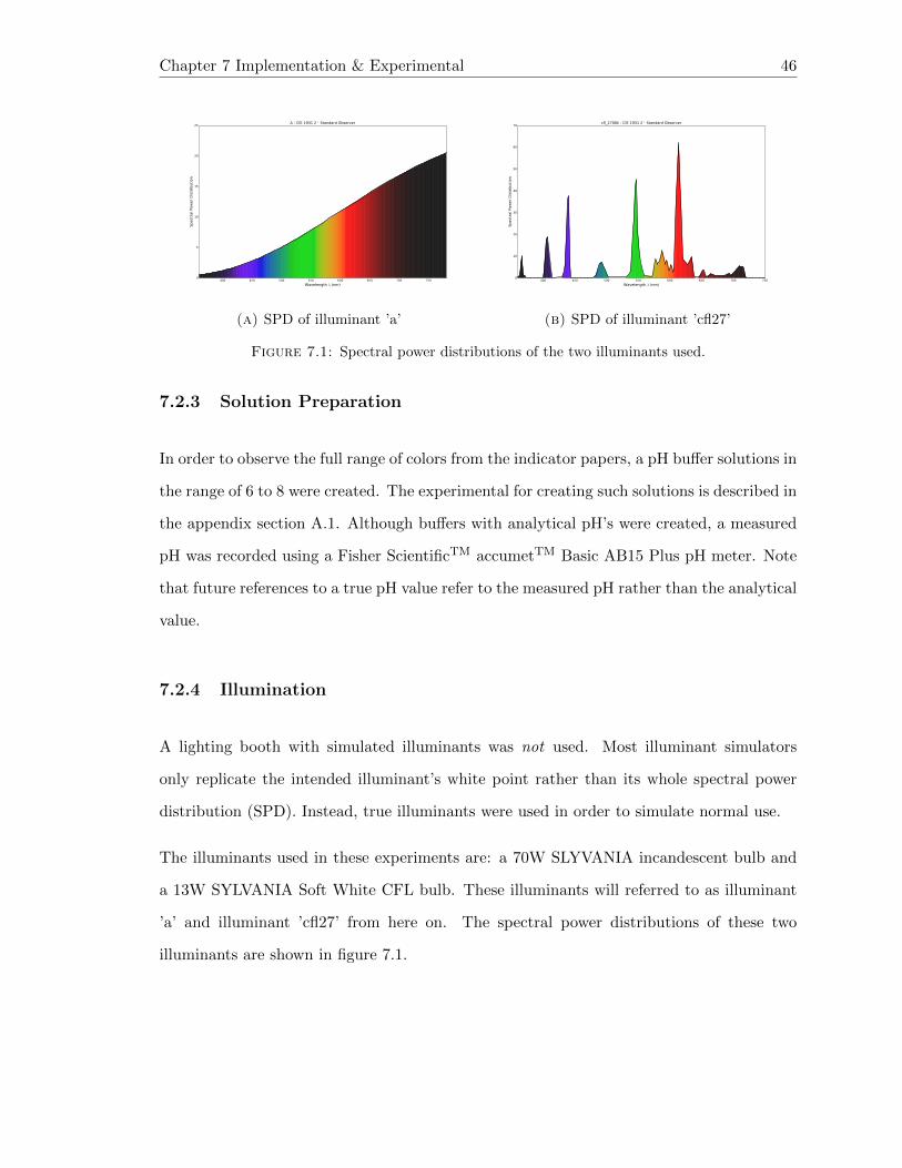
Chapter 7 Implementation & Experimental 46
400 450 500 550 600 650 700 750
Wavelength λ (nm)
0
5
10
15
20
25
Spect
ral Pow
er
Dis
trib
uti
on
A - CIE 1931 2 ◦ Standard Observer
(a) SPD of illuminant ’a’
400 450 500 550 600 650 700 750
Wavelength λ (nm)
0
10
20
30
40
50
60
70
Spect
ral Pow
er
Dis
trib
uti
on
cfl_2700k - CIE 1931 2 ◦ Standard Observer
(b) SPD of illuminant ’cfl27’
Figure 7.1: Spectral power distributions of the two illuminants used.
7.2.3 Solution Preparation
In order to observe the full range of colors from the indicator papers, a pH buffer solutions in
the range of 6 to 8 were created. The experimental for creating such solutions is described in
the appendix section A.1. Although buffers with analytical pH’s were created, a measured
pH was recorded using a Fisher ScientificTM accumetTM Basic AB15 Plus pH meter. Note
that future references to a true pH value refer to the measured pH rather than the analytical
value.
7.2.4 Illumination
A lighting booth with simulated illuminants was not used. Most illuminant simulators
only replicate the intended illuminant’s white point rather than its whole spectral power
distribution (SPD). Instead, true illuminants were used in order to simulate normal use.
The illuminants used in these experiments are: a 70W SLYVANIA incandescent bulb and
a 13W SYLVANIA Soft White CFL bulb. These illuminants will referred to as illuminant
’a’ and illuminant ’cfl27’ from here on. The spectral power distributions of these two
illuminants are shown in figure 7.1.

Chapter 7 Implementation & Experimental 47
7.2.5 Positional Setup
The illumination source is placed roughly 0.6m above the surface of interest at a 35◦ angle
to the surface normal. The imaging device is located roughly ˜0.5m away from the surface
and in line with the surface normal.
7.3 Camera Calibration
In chapter 4, an overview of a general imaging pipeline was given. However, in practice,
different devices are subject to deviations. This is especially true in post-processing when
designers are not as constrained by hardware limitations. With that said, the exact post-
processing procedure of the Nokia N900 camera is left unknown. The technical specification
sheet [7] contains a register map to the gain settings; however, extracting this is much too
inaccessible to be practical. Instead, digital gains will be estimated through a calibration
procedure in order to help correct for any missing post-processing steps.
First, assuming unit digital gain for each color channel, color patches from the Macbeth
ColorChecker chart are simulated for each observed illuminant. Let RGBsim be the matrix
of simulated RGB values for every color patch. The surface reflectance spectra for the
Macbeth ColorChecker color patches are available via [31] and were accessed from [32]’s
interface. Similarly, let RGBobs be the matrix of observed RGB values of each color patch
(details of the data collection are discussed in the previous section 7.2). For N ColorChecker
chart observations (images), both of these matrices will be of shape 24N ×3 since the chart
contains 24 color patches. And of course, the rows of RGBsim and RGBobs correspond to
the same color patch under the same illuminant.

Chapter 7 Implementation & Experimental 48
7.3.1 Linear Scaling
The goal is to find an optimal vector of linear scaling factors, M , such that
Mopt = arg minM
24N−1∑i=0
∑ch∈{R,G,B}
(RGBesti,ch ∗Mch −RGBobsi,ch)2 (7.1)
Implementation-wise, the Nelder-Mead optimization algorithm was used for finding Mopt.
With this particular dataset, Mopt = [2.463, 2.140, 2.628]. This linear scaling result is not
used however. The results from the next section will take its place.
7.3.2 N-way Channel Interactions
Instead of scaling each color channel independently, the output channel can be a linear
combination of all three color channels. Extending this further, the output channel can
even be a linear combination of n-way interactions between channels. These N-way feature
interactions, also known as multisets, are constructed using the multichoose operation. Yet
another name for this concept is combination with replacement. A 2-way multiplicative
interaction for features {R,G,B} would yield the following set of features {R∗R,R∗G,R∗
B,G ∗ G,G ∗ B,B ∗ B} with the lower interactions ({R,G,B}) typically concatenated for
a total of 9 features.
The output of a given color channel, C, is then determined through a linear regression
model:
Cest(x,w) = wTx (7.2)
where C ∈ {R,G,B}, and x = [1, R,G,B,R2, RG,RB,G2, GB,B2] for the above feature-
set. The weights, w, are then solved in least squares optimization as follows
wopt = arg minw
24N−1∑i=0
(Cest(xobsi ,w)− Cobsi)2 (7.3)

Chapter 7 Implementation & Experimental 49
Figure 7.2: Simulated and observed Macbeth ColorChecker arrangements with and with-out an estimated digital gain. 2-way channel interactions are used for this particular digital
gain.
This is repeated for each of the three color channels. Figure 7.2 depicts sample simulations
before and after applying the calibration1 procedure using observed colors of a ColorChecker
chart.
1The term “digital gain” is now a bit of a misnomer in this case. But still refers to the parametersresulting from calibration.

Chapter 8
Results and Discussion
8.1 MAP Estimate Results
Table 8.1 compares the performance of several traditional regression algorithms including
the MAP estimate predicted by the Bayesian network. The regression algorithms used are
as follows: Linear Regression (LR), Support Vector Machine Regression (SVR), Random
Forest Regression (RF), and Gradient Boosted Decision Trees Regresssion (GBDT). The
performance metrics used are the typical ones used for evaluating regression models: Mean
Absolute Error (MAE), Mean Square Error (MSE), and Coefficient of Determination (R2).
Lower values for MAE and MSE are desired, whereas a higher R2 is better. Refer to
appendix section C for details on performance metrics.
The training regimen for this experiment is to train only on observations taken under one
illuminant. Validation will then be executed on samples under another illuminant. This
is to simulate data collection in a lab for prediction in another environment. The MCMC
model used for data augmentation will also only have access to observations taken under
the training illuminant. The entire training and validation procedure is repeated 10 times
with different randomization seeds. The final performance results are the average of these
10 runs.
50

Chapter 8 Results and Discussion 51
TrainingIllum
Model MAE MSE r2
a
LR 0.32320 0.15280 0.55565RF 0.27006 0.11430 0.66762
SVR 0.29319 0.13332 0.61232GBDT 0.37369 0.19532 0.43202MAP 0.22899 0.10346 0.69913
cfl27
LR 0.22147 0.07529 0.78107RF 0.24746 0.09328 0.72874
SVR 0.47939 0.31055 0.09694GBDT 0.26505 0.10598 0.69182MAP 0.21968 0.07380 0.78539
Table 8.1: Comparison of regression performances for various models trained on datafrom a single illuminant. Bold values denote the best performance for a given evaluation
metric and training illumination.
Table 8.1 shows that the MAP estimate of the proposed Bayesian network performs the best
over the given performance metrics. This is not a surprising result; even though all models
were trained with the same data, the Bayesian network, by construction, contains more
information of the imaging device, illumination, and surface material. The problem with
the other regression models is that since they’re only trained on one illuminant, they never
get to observe the variations caused by another illuminant. On the other hand, while the
Bayesian network is also only trained on one illuminant, it has the SPD of other illuminants
in its look-up table. Thus, it considers the possibility of various observed RGB values from
other illuminants.
While the MAP estimate of the Bayesian network outperforms the other models in terms
of regression metrics, it suffers in prediction time. This is mainly because the Bayesian
network needs to traverse through the imaging pipeline (computationally expensive) every
time data is to be simulated. As of the current software implementation, each MAP estimate
takes roughly 1000x longer than the slowest of the regression models 1. Admittedly, with
the current implementation, this is not ready to be used in product as-is. The next section
discusses results for a more production-ready strategy using data augmentation.
1Random forest regressor with 32 estimators takes on the order of 0.1s per prediction. MAP estimatetakes on the order of 100s per prediction – very slow!

Chapter 8 Results and Discussion 52
TrainingIllum
Model MAEMAE(da)
MSEMSE(da)
r2r2
(da)
a
LR 0.32360 0.32014 0.15257 0.14557 0.55634 0.57670RF 0.28701 0.26032 0.13458 0.10852 0.60864 0.68442
SVR 0.30202 0.31688 0.15846 0.16481 0.53921 0.52073GBDT 0.26723 0.26740 0.11445 0.11107 0.66717 0.67701
cfl27
LR 0.23248 0.18083 0.08310 0.05379 0.75836 0.84359RF 0.26219 0.29372 0.10932 0.16000 0.68211 0.53473
SVR 0.52478 0.34138 0.37601 0.18820 -0.09342 0.45272GBDT 0.26734 0.27811 0.10537 0.14365 0.69358 0.58227
Table 8.2: Regression performance for various models trained on data from a singleilluminant compared against models trained with augmented data. Metrics labeled with’da’ denote the use of data augmentation. Bold values denote the best performance for a
given evaluation metric and training illumination.
8.2 Data Augmentation Results
Table 8.2 compares the performance of several traditional regression algorithms with and
without the use of data augmentation via MCMC. The same regression models and per-
formance metrics will be used as in section 8.1. And again, as in section 8.1, the training
regimen for this experiment is to train only on observations taken under one illuminant. Val-
idation will then be executed on samples under another illuminant. The MCMC model used
for data augmentation will also only have access to observations taken under the training
illuminant.
Data augmentation is carried out as according to section 6.4 to generate 500 augmenta-
tion samples. Since the original dataset is small in comparison (40 samples), bootstrap
resampling of the original data is used. This is to prevent the augmentation samples from
over biasing while still have enough augmentation samples to explore the variances in the
MCMC model. The ratio of resampled original observations to the number of augmentation
samples is a free parameter to be explored; a ratio of 20 was used in this case. To make
it a fair comparison between non-augmented and augmented datasets, the same bootstrap
resampling is done in both cases (with the same seed for randomization). The entire train-
ing and validation procedure is repeated 10 times with different randomization seeds. The
final performance results are the average of these 10 runs.

Chapter 8 Results and Discussion 53
Table 8.2 shows that 14 of the 24 possible comparisons yielded a beneficial impact from
using MCMC data augmentation. More importantly, the best performing model for a given
training illuminant and performance metric was the result of using data augmentation.
Admittedly, data augmentation did not improve all performance metrics for all models.
However, improvement of the best score in every situation suggests that the information
provided from data augmentation can be useful. And unlike using the MAP estimate (results
shown in section 8.1), using data augmentation introduced very little additional time for
prediction. Instead, most of the work is front-loaded into generating the augmentation
data. This makes data augmentation via MCMC samples a very attractive method of
introducing the information from the Bayesian network into a fast-predicting regression
model for production-facing systems.
8.3 Approximated Posterior
Lastly, an attractive feature of Bayesian inference is that we have an estimated posterior
distribution. Unfortunately, since this is such a unique form of a prediction, it is difficult
to properly quantify its performance. Table 8.3 shows that the approximated posterior
at least outperforms a uniform distribution over the pH range 6 to 8. The performance
metrics include Hellinger distance, Kullback Leibler (KL) divergence, and the negative
log probability of the true pH. For the Hellinger distance and KL divergence, a Normal
distribution centered around the true pH with a standard deviation of 0.01 was used as the
true distribution. This standard deviation represents the precision of the pH meter used to
measure the true pH of the solution. For all three of these metrics, a lower value indicates
better performance. Refer to appendix section C for details on performance metrics.
The metrics are then aggregated over all observations. Both the mean and median are shown
in table 8.3 as indicated in parenthesis next to the distribution name. Unsurprisingly, the
approximated posterior outperforms the uniform distribution. Additionally, the median of
scores are better than the mean of scores, especially for logloss. This indicates that there
are a few instances where the approximated posterior was very confidently incorrect. But

Chapter 8 Results and Discussion 54
Hellingerdist
KLdiv
logloss
MCMC Posterior(Mean)
0.87884 3.78831 0.57696
MCMC Posterior(Median)
0.86730 2.97511 -0.23332
Uniform(Mean)
0.91963 3.93430 0.69315
Uniform(Median)
0.91765 3.88439 0.69315
Table 8.3: Comparison of the approximated posterior with a uniform distribution overpH 6 to 8. Both the mean and median over all performances are provided for the MCMC
posterior.
6.0 6.5 7.0 7.5 8.0pH
0.0
0.5
1.0
1.5
2.0
2.5Observation #20
Approx. PosteriorTrue pH
(a)
6.0 6.5 7.0 7.5 8.0pH
0.0
0.5
1.0
1.5
2.0
2.5
3.0
3.5Observation #7
Approx. PosteriorTrue pH
(b)
Figure 8.1: Hand-picked examples of some estimated posteriors via MCMC. 8.1a shows awell approximated posterior. 8.1b exemplifies an unfortunate case where the approximated
posterior was overly confident in values very close to the true pH.
most of the estimates performed much better; in fact, half of the estimates yielded a logloss
of less than -0.23332. Figure 8.1 shows two example posterior estimations. And in figure
8.1b, an example of this overconfident behavior is shown. Note that although this yields a
poor logloss, the corresponding MAP estimate is actually not far off.

Chapter 9
Conclusion
In this thesis, we synthesized image data for a bromothymol blue pH indicator via surface
reflectance spectra generation in conjunction with a simulated digital camera pipeline. The
model itself was realized as a Bayesian network which allowed for MAP estimates and
posterior approximations via MCMC sampling. The model was then used to predict the pH
of solutions given the image of a pH indicator test strip dipped in said solution. Because this
model made better use of available domain knowledge, it performed better than uninformed
traditional regression models. A data augmentation scheme was also devised in order to
easily ensemble the Bayesian model into other models – improving performance by sharing
domain knowledge. Hopefully this work will remind others that domain knowledge is very
useful, especially in the case of small data.
9.1 Future Work
As an exemplary case, a bromothymol blue based pH indicator was used to validate the
proposed framework. It should not take much to extend the model to work other other
colorimetric indicators. For example, there are many colorimetric indicators used for uri-
nalysis, including indicators signaling levels of: nitrite, leukocyte, protein, ketone, specific
gravity, bilirubin, and glucose.
55

Chapter 9 Conclusion 56
In section 6.2, fitting the model using direct measurements from a reflectance spectropho-
tometer was mentioned. In fact, this was the original plan for this project. This is also
probably the preferred method for real life applications. However, a reflectance spectropho-
tometer could not be acquired due to a lack of budget.
One of the great benefits of Bayesian analysis is that the model can be easily improved
upon additional domain knowledge. Throughout the building of the Bayesian network
used, many simplifying assumptions were made. For example, when modeling the imaging
physics, many assumptions were taken due to a lack of device specifications or a lack of
measuring hardware. Or for example, the absorbance spectra was modeled using a mixture
of Gaussian functions. If additional knowledge is obtained regarding the imaging device or
chemical indicator, these assumptions could very well be worked out to be more exact.
In terms of software, in this work, pymc2 [27] was used for sampling and computation of
posteriors. However, development for pymc2 has basically halted indefinitely in favor of
pushing pymc3 [33]. There are plans to use pymc3 which makes use of Theano [34] (can
leverage GPU for computations) and offers more MCMC methods such as Hamiltonian
Monte Carlo.

Appendix A
Experiment Preparation
A.1 pH Buffer Creation
A.1.1 Objective
Stock solutions of citric acid and sodium phosphate are to be prepared. Various proportions
of these two solutions will be mixed in order to yield buffer solutions of various pH.
A.1.2 Procedure
1. 500 mL of 0.2 mol/L Sodium hydrogen phosphate (Na2HPO4) solution of was prepared
by dissolving 17.7988 g of Na2HPO4 · 2 H2O (177.988 g/mol) in deionized water, and
then diluting the solution to the final volume with deionized water.
2. 250 mL of 0.1 mol/L Citric acid (C6H8O7) solution of was prepared by dissolving
4.8031 g of C6H8O7 (192.122 g/mol) in deionized water, and then diluting the solution
to the final volume with deionized water.
3. Reference table A.1 to form a range of pH buffers using various ratios of sodium
hydrogen phosphate and citric acid
4. For each solution created, record a measured pH via a pH meter
57

Appendix A Experiment Preparation 58
pH 0.1M Citric Acid [mL] 0.2 Na2HPO4 [mL]
5.6 42.00 58.005.8 39.55 60.456.0 36.85 63.156.2 33.90 66.106.4 30.75 69.256.6 27.25 72.756.8 22.75 77.257.0 17.65 82.357.2 13.05 86.957.4 9.15 90.857.6 6.35 93.65
Table A.1: Ratios of citric acid and sodium phosphate used to create gradation of pHbuffers. Taken from [8]

Appendix B
Relevant Source Code
B.1 Bayesian Network Model
import pymc as pm
import numpy as np
import cPickle as pickle
import colour
import sys
if ’../spec -est/’ not in sys.path:
sys.path.append(’../spec -est/’)
import data.data_load as dl
import imcapture
reload(imcapture)
from imcapture.camera import Camera
import gen.surface as gs
from scipy.stats import norm
from sklearn.preprocessing import LabelEncoder
import warnings
warnings.simplefilter("ignore", category=DeprecationWarning)
def logistic(x, x0, k):
return 1./(1 + np.exp(-k*(x-x0)))
59

Appendix B Relevant Source Code 60
def rlogistic(x, x0, k):
# Logistic mirrored over y axis
return 1. - 1./(1 + np.exp(-k*(x-x0)))
def fulllogistic(x, L, x0 , y0, k):
return L/(1 + np.exp(-k*(x-x0))) + y0
def rfulllogistic(x, L, x0, y0, k):
return L*(1 - 1./(1 + np.exp(-k*(x-x0)))) + y0
SEED = 322
np.random.seed(SEED)
l = np.arange (400, 725, 1) # static wavelengths
l_spd_shape = colour.SpectralShape(start=l.min(), end=l.max(), steps=l[1]-l[0])
spd_cfl_d = pickle.load(open(’../ btb_dataset/saved/sylvania_spd_d.p’))
e_d = {
# Normalizing SPDs
’CFL27’: spd_cfl_d [2700]. clone () * 467.62636719 ,
’CFL35’: spd_cfl_d [3500]. clone () * 516.17080078 ,
’A’: colour.ILLUMINANTS_RELATIVE_SPDS[’A’].clone () * 0.08480415 ,
}
# illum_types = [’a’, ’cfl27 ’, ’cfl35 ’]
illum_types = [’a’, ’cfl27’]
le_illum = LabelEncoder ().fit(illum_types)
n_illums = len(illum_types)
p_illum = np.ones(n_illums , dtype=float) / n_illums
def get_illum_colour(illum_str):
interp_meth = ’linear ’
e = e_d[illum_str.upper()]. clone()
e_n = e.clone ().align(l_spd_shape , method=interp_meth)
e_retvals = e_n.values
e_retvals[e_retvals < 0] = 0
return e_retvals

Appendix B Relevant Source Code 61
# Preload illuminant SPD ’s we don ’t waste time doing it over and over again
illum_spd_d = {
illum: get_illum_colour(illum) for illum in illum_types
}
def get_illum_colour_preloaded(illum_str):
return illum_spd_d[illum_str]
# These can also be stochastic (example as commented ), but that ’s quite overkill
sigma_p_loc = 1 # pm.Uniform(’ sigma_p_loc ’, 0, 2, size =2)
sigma_p_scale = 0.5 # pm.Uniform(’ sigma_p_scale ’, 0, 1, size =2)
sigma_p_height = 0.01 # pm.Uniform(’ sigma_p_height ’, 0, 0.04 , size =2)
cam_name = ’Nokia N900’
dist_src_surf = 0.6 # distance from source to surface [m]
tot_sterad = 4 * np.pi * dist_src_surf ** 2
area = 2e-3
surf_sterad = area / tot_sterad
params_d = pickle.load(open(’./ params_by_train_illum.p’, ’rb’))
def make_model(rgb_obs=None , t_exp =1/20. , iso=100,
fitted=True , illum_ass=None ,
fitted_params=None):
"""
:param rgb_obs: observed rgb value (optional)
:param t_exp: exposure time of camera [s]
:param iso: digital iso of camera
:param fitted: if ‘True ‘, multimodal params will be dependent on ph
:param illum_ass: if fitted is ‘False ‘, training illumination assignment should
be provided
:param fitted_params: custom fitted params -- must unpack as 3 iterables of
length (4, 2, 2)
or the appropriate illum str (for the params fitted by sep training illums)
"""
# Dealing with params
if fitted_params is None:
p_mu_peak_loc_0 = [5.8471932 , 6.64086137 , 430.21040582 , 2.64186295]
p_mu_peak_height_0 = [8.04, 3.41]

Appendix B Relevant Source Code 62
p_mu_peak_height_1 = [7.64, 2.11]
elif isinstance(fitted_params , str):
p_mu_peak_loc_0 , p_mu_peak_height_0 , p_mu_peak_height_1 = params_d[
fitted_params]
else:
p_mu_peak_loc_0 , p_mu_peak_height_0 , p_mu_peak_height_1 = fitted_params
# ###############################################################
# Illum
# ###############################################################
if illum_ass is None:
illum_assignment = pm.Categorical(’illum_assignment ’, p_illum)
else:
illum_assignment = illum_ass
@pm.deterministic
def illum_spectra(illum_enc=illum_assignment):
""" Get the spectra associated with an illumination type """
illum_str = le_illum.inverse_transform(illum_enc)
return get_illum_colour_preloaded(illum_str)
# ###############################################################
# ph
# ###############################################################
if fitted:
ph = pm.Uniform(’ph’, 6.0, 8.0)
# ###############################################################
# Surface Generation
# ###############################################################
if fitted:
@pm.deterministic
def mu_peak_locs(ph=ph):
"""
:param ph: ph of the solution
:return: the peak locations [wavelengths] of the abs spectra
"""
v = [ # fitted?
lambda ph: rfulllogistic(ph, *p_mu_peak_loc_0),
lambda ph: 615,
]
locs = np.array ([v_i(ph) for v_i in v])

Appendix B Relevant Source Code 63
return locs
peak_locs = pm.Normal(’peak_locs ’, mu=mu_peak_locs , tau=sigma_p_loc **-2)
peak_scales = pm.Normal(’peak_scales ’, size=2, mu=50, tau =0.5** -2)
@pm.deterministic
def mu_peak_heights(ph=ph):
"""
:param ph: ph of the solution
:return: the heights of the peaks (absorption) of the abs spectra
"""
v = [ # Based on logistic fit
lambda ph: rlogistic(ph , *p_mu_peak_height_0),
lambda ph: logistic(ph, *p_mu_peak_height_1),
] # h functions to get modal heights based on parameter (ph)
h = np.array([v_i(ph) for v_i in v])
return h
peak_heights = pm.Normal(’peak_heights ’, mu=mu_peak_heights , tau=
sigma_p_height **-2)
else:
peak_locs = pm.Normal(’peak_locs ’, mu=[430 , 615], tau=[2**-2, 1** -2])
# peak_scales = pm.Uniform(’ peak_scales ’, size =2, lower =40, upper =55)
peak_scales = pm.Normal(’peak_scales ’, size=2, mu=50, tau =0.5** -2)
peak_heights = pm.Uniform(’peak_heights ’, size=2, lower =0.0, upper =1.0)
@pm.deterministic
def multimodal_spec(mu=peak_locs ,
sigma=peak_scales ,
h=peak_heights ,
wvlns=l):
"""
Generates a spectra over the given wvlns
with modes at mu and spread of each mode given by sigma
h denotes the peak heights
"""
pk_wt = h * sigma * np.sqrt (2*np.pi)
dists = norm(loc=mu[None , :], scale=sigma[None , :])
wvlns_obs_shape = np.concatenate (( wvlns.shape , np.ones(len(mu.shape))))
s = pk_wt * dists.pdf(wvlns.reshape(wvlns_obs_shape))

Appendix B Relevant Source Code 64
s_comb = np.sum(s, axis =1)
# return s_comb , wvlns
return s_comb
@pm.deterministic
def ref_spec(abs_spec=multimodal_spec):
albedo =0.7
return albedo / 10 ** abs_spec
# ###############################################################
# Scene Capture
# ###############################################################
@pm.deterministic
def radiance(ref_spec=ref_spec ,
illu_spec=illum_spectra):
rad = ref_spec * illu_spec * surf_sterad # from surface
return rad
@pm.deterministic
def image(rad=radiance):
some_cam = Camera(model=cam_name ,
wb_mode=’none’,
t_exp_mode=’manual ’,
t_exp=t_exp ,
iso=iso ,
verbose=False)
# pretend all 4 bayer filter arrays get the same irradiance
rad_bayer = np.tile(rad[None , None , :], [8, 8, 1])
# rad_bayer = np.tile(rad[None , None , :], [16, 16, 1])
img = some_cam.transform(rad_bayer , l)
return img
@pm.deterministic
def img_avg(img=image):
return img.mean(axis =0).mean(axis =0)
# ###############################################################
# Observation
# ###############################################################
# rgb_prec = np.tile (5**-2, 3)
rgb_prec = np.tile (15**-2, 3)

Appendix B Relevant Source Code 65
if rgb_obs is None:
imaged_obs = pm.Normal("img_obs", img_avg , rgb_prec)
else:
imaged_obs = pm.Normal("img_obs", img_avg , rgb_prec , value=rgb_obs , observed=
True)
return locals ()
B.2 Camera Model
__author__ = ’jason’
import numpy as np
from scipy.interpolate import interp1d
from scipy import constants
import matplotlib.pyplot as plt
from scipy.ndimage.filters import convolve
import data.data_load as dl
# import cv2
from skimage import color
from scipy.stats import multivariate_normal
import colour
"""
Relevant Literature
http :// white.stanford.edu/~brian/papers/pdc/2012 -DCS -OSA -Farrell.pdf
"""
class Camera ():
def __init__(self , ** kwargs):
# todo: I think it would be cool if verbose was an iterable
# of which stages to be verbose about
"""
:param model: camera model name
:param wb_mode: white balance mode (currently supports ’auto’ and ’none ’)
:param t_exp: Init Exposure time [s] (for ’live preview ’)
:param t_exp_mode: Exposure mode: ’auto’ or ’manual ’.
If manual , exposure time will be locked to ‘t_exp ‘
:param iso: iso film equivalent of sensor (used as voltage analog gain)

Appendix B Relevant Source Code 66
:param dig_gain: digital gain (default to calibrated gains)
:param verbose: verbosity
:return: Camera object
"""
param_defaults = {
’model’: ’unknown ’,
’wb_mode ’: ’auto’,
’t_exp’: 1/250. ,
’t_exp_mode ’: ’auto’,
’iso’: 100,
’dig_gain ’: None ,
’verbose ’: False ,
}
for (prop , default) in param_defaults.iteritems ():
setattr(self , prop , kwargs.get(prop , default))
self.optics = Optics(verbose=self.verbose)
self.sensor = Sensor(t_exp=self.t_exp , iso=self.iso , cam_name=self.model ,
verbose=self.verbose)
self.preproc = PreProc(verbose=self.verbose)
self.postproc = PostProc(wb_mode=self.wb_mode , dig_gain=self.dig_gain ,
verbose=self.verbose)
def transform(self , irrad , l=None):
"""
Transforms irradiance incident at sensor to a captured image
Wraps the pipeline containing optics , sensor noise ,
preprocessing for auto exposure.
:param irrad: irradiance incident at sensor either as colour.SPD object or
array (H x W x n_lambda)
if an array is given , ‘l‘ must also be given
:param l: corresponding wavelengths of ‘irrad ‘ if ‘irrad ‘ is given as an
array
:return: Captured image
"""
if hasattr(irrad , ’clone ’):
irrad = irrad.clone()
irrad2 = self.optics.transform(irrad)
# Raw capture in live view

Appendix B Relevant Source Code 67
# v_pre = self.sensor.transform (irrad2 , l)
v = self.sensor.transform(irrad2 , l)
if self.t_exp_mode == ’auto’:
# todo: wrap this tolrance -based iterative procedure
# or calculate optimal t better
for ii in range (5):
# Getting the optimal exposure time from live view
self.t_exp = self.preproc.autoexpose_pre(
v, f=self.optics.f_num , t=self.t_exp)
# Re -exposure using optimal exposure time
self.sensor.t_exp = self.t_exp
v = self.sensor.transform(irrad2 , l)
# Need to switch case for bayer post proc if sensor CFA is bayer
im = self.postproc.transform(
v, f=self.optics.f_num , t=self.t_exp)
# repeat given autoexposure settings
return im
def set_shutter(self , t_exp):
self.t_exp = t_exp
self.sensor.t_exp = t_exp
def set_iso(self , iso):
self.iso = iso
self.sensor.iso = iso
class Optics ():
def __init__(self , ** kwargs):
"""
:param f_num: f-number of the optical system (relative aperature)
:param focal_len: focal length of lens
:param lens_trans: transmissivity of each wavelength through optical system
:param verbose: verbosity
:return:
"""
param_defaults = {
’f_num’: 2.8, #4.,
’focal_len ’: 5.2, # 3.,

Appendix B Relevant Source Code 68
’lens_trans ’: 1., # perfect for all wavelengths
’verbose ’: False ,
}
for (prop , default) in param_defaults.iteritems ():
setattr(self , prop , kwargs.get(prop , default))
def transform(self , rad):
"""
Takes the radiance incident at the camera lens and
transforms it into the irradiance incident at the
camera sensor
"""
irradiance = rad * np.pi * self.lens_trans / (4 * self.f_num **2)
return irradiance
class Sensor ():
def __init__(self , ** kwargs):
param_defaults = {
’t_exp’: 1/250. , # Exposure time [s]
’cam_name ’: ’unknown ’,
# ISA Properties
’cfa_type ’: ’bayer’, # bayer or foveon
’pattern ’: ’gbrg’, # only valid for Bayer
’shape’: None , # tbd by data
# Pixel Structure
’w_px’: 2.2e-6, # width of photosite (2.2 um)
’h_px’: 2.2e-6, # height of photosite (2.2 um)
# ’area_ps ’: (2.2e -6) *(2.2e -6) , # m^2s
’fill_fact ’: 0.45, # Fill factor
’well_cap ’: 9000, # well capacity [# electrons]
# Electron conversion
’v_swing ’: 1.8, # voltage swing [V]
# ’gain_analog ’: 1.0, # analogous to changing ISO
’iso’: 100., # use this to derive gain_analog
# Noise Figures
’darkv_dt ’: 4.68e-3, # [V/s] (4.68 mV/s)

Appendix B Relevant Source Code 69
’sigma_readv ’: 0.89e-3, # [V] (0.89 mV)
’dsnu’: 0.83e-3, # [V]
’prnu’: 0.736,
’verbose ’: False ,
}
for (prop , default) in param_defaults.iteritems ():
setattr(self , prop , kwargs.get(prop , default))
# Get convert iso to gain_analog (assume linear)
self.gain_analog = self.iso / 100.
# Color Filter Sensitivities ( transmissivities )
# self.rho , self.l_rho = dl. load_cameras (cam_name=self.cam_name)
self.rho = dl.load_cameras(cam_name=self.cam_name)
# Pixel Structure
self.area_ps = self.w_px * self.h_px # m^2s
# Electron conversion
self.gain_conversion = self.v_swing / self.well_cap # [V/e]
# # Noise Figures
self.darkv = self.darkv_dt * self.t_exp
self.darke = self.darkv / self.gain_conversion
def transform(self , irradiance , l=None , interp_meth=’linear ’):
"""
Takes the irradiance incident at the camera sensor and
transforms it into a voltage reading
:param irradiance: H W #l
:param l: wavelengths of ‘irradiance ‘ if it is given as array rather than SPD
object
"""
if hasattr(irradiance , ’wavelengths ’):
l = irradiance.wavelengths
l_spd_shape = irradiance.shape
irradiance = irradiance.values
# don ’t transpose if SPD object is given
# it’s values will come in shape #l H W

Appendix B Relevant Source Code 70
else:
l_spd_shape = colour.SpectralShape(start=l.min(), end=l.max(), steps=l
[1]-l[0])
irradiance = np.transpose(irradiance)
n_phot = self.photon_counting(irradiance , l)
rho_n = self.rho.clone ().align(l_spd_shape)
# import pdb; pdb.set_trace ()
rho_bayer = self.get_bayer_pattern(
rho_n.values , irradiance.shape)
n_e_tot = self.photon_to_e(n_phot , rho_bayer , l)
v_out = self.read_voltage(n_e_tot)
if self.verbose:
print ’rho bayer shape:’, rho_bayer.shape
return v_out
def get_bayer_pattern(self , rho , s_shape):
"""
(#l, 3) -> tiled (2, 2, #l)
where l is the wavelength array of rho
it is assumed that the order of the channels in rho is RGB
:param rho: [#l, 3] sensor sensitivities
:param s_shape: [#l, w, h] sensor/scene shape
"""
pattern = np.array ([[’b’, ’g’], [’g’, ’r’]])
ch_sens = {ch: rho[:, ii] for ii, ch in enumerate ([’r’, ’g’, ’b’])}
tile = np.array ([[ ch_sens[c] for c in r] for r in pattern ])
mult = np.r_[np.array(s_shape)[1:]/2 , 1]
tiled_bayer = np.tile(tile , mult)
ch_masks = {
ch: np.tile(pattern == ch , mult [: -1])
for ch in [’r’, ’g’, ’b’]
}
return np.transpose(tiled_bayer , [2, 0, 1])
def photon_counting(self , irradiance , l):
"""
:returns n_phot: the number of photons in each wavelength bin
incident before the pixel filter
"""

Appendix B Relevant Source Code 71
Phi = irradiance_to_photonflux(irradiance , l)
# Expected number of photons at a particular wavelength bin at a photosite
mu_phot = Phi * self.area_ps * self.fill_fact * self.t_exp
mu_phot_tot = np.sum(mu_phot , axis =0) # sum over wavelength dimension
if self.verbose:
print ’Total photons incident at the sensitive part of a photosite:’,
mu_phot_tot
# n_phot_tot = np.random.poisson(mu_phot_tot , mu_phot_tot .shape)
# n_phot = n_phot_tot * mu_phot / mu_phot_tot
# TODO: need guard against mu_phot < 0
n_phot = np.random.poisson(mu_phot , mu_phot.shape)
return n_phot
def photon_to_e(self , n_phot , rho_n , l):
"""
:param n_phot: [#l, w, h] number of photons incident at each sub -pixel
:param rho_n: [#l, w, h] the sensitivities at each sub -pixel of the sensor.
usually this is the bayer tiled sensitivities
:param l: [#l] wavelengths axis for integration
(allows for nonuniform spacing)
:return: [w, h] net electrons at each electron -well (sub -pixel)
"""
# prod = n_phot [:, :, :, None] * rho_n # foveon filters with built in 3ch
dimensionality
prod = n_phot * rho_n
f = np.trapz(prod , l, axis =0)
# Adding Dark Electrons
mu_darke = self.darkv / self.gain_conversion
# n_darke = np.random.poisson(mu_darke , f.shape [: -1])
n_darke = np.random.poisson(mu_darke , f.shape)
# print ’Number of Dark Electrons :’, n_darke
# Total number of electrons collected in the well
# n_e_tot = f + n_darke [:, :, None] # todo: Need to change when/if bayer
sensor is used since each ’channel ’ is a psite
n_e_tot = f + n_darke # Need to change when/if bayer sensor is used since
each ’channel ’ is a psite

Appendix B Relevant Source Code 72
# Saturate at the well capacity
n_e_tot = np.clip(n_e_tot , 0, self.well_cap)
# print n_e_tot
return n_e_tot
def read_voltage(self , n_e):
"""
Reads the voltage at each of the photodetector electron wells
"""
v = n_e * self.gain_conversion
# Read noise
v_read = v + np.random.normal(loc=0, scale=self.sigma_readv , size=v.shape)
# print v, v_read
v_gain = v_read * self.gain_analog
# Quantization in A/D converter
v_out = np.round (255.0 * v_gain/self.v_swing)
# v_out = np.round(v_gain)
# print ’Quantized:’, v_gain , ’\n’, v_out
return v_out
class PostProc ():
def __init__(self , ** kwargs):
param_defaults = {
’wb_mode ’: ’auto’,
’dig_gain ’: None ,
’verbose ’: False ,
}
for (prop , default) in param_defaults.iteritems ():
setattr(self , prop , kwargs.get(prop , default))
# Demosaicing
pass
def transform(self , v, ** kwargs):
"""
Takes the image read from the sensor and applies
demosaicing , autoexposure , and whitebalancing

Appendix B Relevant Source Code 73
In the case of autoexposure , an additional image capture
at a different exposure time is usually required
Careful because if the gain is off , there is going to be
a bias in the exposure time - giving a bias to our shot noise
So it’s important to make sure that our radiance & power physics
calculations are approximately correct
"""
im_demosaiced = self.demosaic(v)
if self.wb_mode == ’none’:
im_bal = im_demosaiced
# cal_gains = np.array ([ 1.19593693 , 1.0306226 , 1.37649275]) # linear
scaling full cc for n900
cal_gains = np.array([ 1.07456815 , 0.9396017 , 1.38019858]) # linear
scaling neutrals for n900
cal_gains_wgam = np.array ([ 1.0423342 , 0.79974847 , 1.15488642 ,
0.61960791 , 0.70029919 ,
0.86072571]) # gains with gamma on each channel
cal_gains_1waylr = np.array ([[ 1.08447801 , 0.07256105 , -0.85822128 ,
51.18274866] ,
[ -0.32649478 , 1.31924785 , -0.32897496 , 30.60182154] ,
[ -0.25944955 , -1.03393193 , 4.04289506 , 14.28572824]])
cal_gains_2waylr = np.array ([[ 2.28865730e+00, -3.93256173e-01,
-1.69312088e+00,
-6.72633377e-03, 4.63322220e-03, 2.56866551e-03,
4.44663398e-03, -2.67880772e-02, 3.52265125e-02,
3.21708138e+01],
[ -6.82105489e-01, 2.33637664e+00, 5.45327398e-02,
1.81278474e-03, -3.19408513e-03, 2.77124607e-03,
-1.93979485e-04, -1.40594490e-02, 1.39335808e-02,
3.23400753e+00],
[ -5.23250775e-01, -1.24479313e+00, 6.19805240e+00,
3.26686300e-03, -6.32079725e-03, -1.17121928e-03,
-2.30083157e-03, 3.79119792e-02, -6.31263566e-02,
-1.19603304e+01]]) # 2 way channel interactions for n900
if self.dig_gain is None:
# dig_gain = cal_gains
# dig_gain = cal_gains_wgam
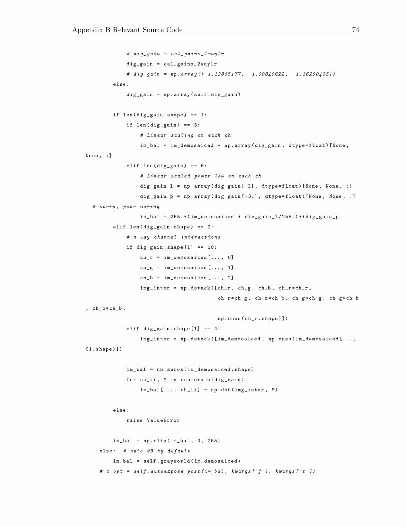
Appendix B Relevant Source Code 74
# dig_gain = cal_gains_1waylr
dig_gain = cal_gains_2waylr
# dig_gain = np.array ([ 1.13865177 , 1.00849622 , 1.16290435])
else:
dig_gain = np.array(self.dig_gain)
if len(dig_gain.shape) == 1:
if len(dig_gain) == 3:
# Linear scaling on each ch
im_bal = im_demosaiced * np.array(dig_gain , dtype=float)[None ,
None , :]
elif len(dig_gain) == 6:
# Linear scaled power law on each ch
dig_gain_l = np.array(dig_gain [:3], dtype=float)[None , None , :]
dig_gain_p = np.array(dig_gain [-3:], dtype=float)[None , None , :]
# sorry , poor naming
im_bal = 255.*( im_demosaiced * dig_gain_l /255.) ** dig_gain_p
elif len(dig_gain.shape) == 2:
# n-way channel interactions
if dig_gain.shape [1] == 10:
ch_r = im_demosaiced [..., 0]
ch_g = im_demosaiced [..., 1]
ch_b = im_demosaiced [..., 2]
img_inter = np.dstack ([ch_r , ch_g , ch_b , ch_r*ch_r ,
ch_r*ch_g , ch_r*ch_b , ch_g*ch_g , ch_g*ch_b
, ch_b*ch_b ,
np.ones(ch_r.shape)])
elif dig_gain.shape [1] == 4:
img_inter = np.dstack ([ im_demosaiced , np.ones(im_demosaiced [...,
0]. shape)])
im_bal = np.zeros(im_demosaiced.shape)
for ch_ii , M in enumerate(dig_gain):
im_bal [..., ch_ii] = np.dot(img_inter , M)
else:
raise ValueError
im_bal = np.clip(im_bal , 0, 255)
else: # auto WB by default
im_bal = self.grayworld(im_demosaiced)
# t_opt = self. autoexpose_post (im_bal , kwargs[’f ’], kwargs[’t ’])
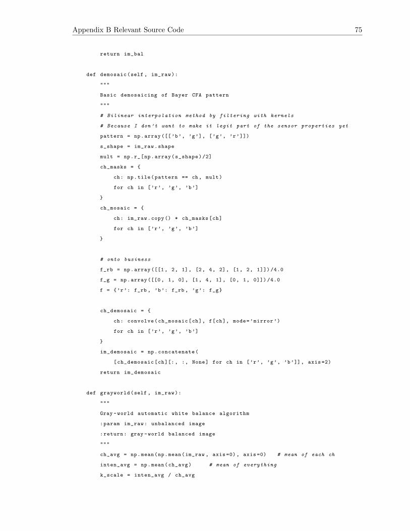
Appendix B Relevant Source Code 75
return im_bal
def demosaic(self , im_raw):
"""
Basic demosaicing of Bayer CFA pattern
"""
# Bilinear interpolation method by filtering with kernels
# Because I don ’t want to make it legit part of the sensor properties yet
pattern = np.array ([[’b’, ’g’], [’g’, ’r’]])
s_shape = im_raw.shape
mult = np.r_[np.array(s_shape)/2]
ch_masks = {
ch: np.tile(pattern == ch , mult)
for ch in [’r’, ’g’, ’b’]
}
ch_mosaic = {
ch: im_raw.copy() * ch_masks[ch]
for ch in [’r’, ’g’, ’b’]
}
# onto business
f_rb = np.array ([[1, 2, 1], [2, 4, 2], [1, 2, 1]]) /4.0
f_g = np.array ([[0, 1, 0], [1, 4, 1], [0, 1, 0]]) /4.0
f = {’r’: f_rb , ’b’: f_rb , ’g’: f_g}
ch_demosaic = {
ch: convolve(ch_mosaic[ch], f[ch], mode=’mirror ’)
for ch in [’r’, ’g’, ’b’]
}
im_demosaic = np.concatenate(
[ch_demosaic[ch][:, :, None] for ch in [’r’, ’g’, ’b’]], axis =2)
return im_demosaic
def grayworld(self , im_raw):
"""
Gray -world automatic white balance algorithm
:param im_raw: unbalanced image
:return: gray -world balanced image
"""
ch_avg = np.mean(np.mean(im_raw , axis =0), axis =0) # mean of each ch
inten_avg = np.mean(ch_avg) # mean of everything
k_scale = inten_avg / ch_avg

Appendix B Relevant Source Code 76
# print k_scale
bal = im_raw * k_scale[None , None , :]
if self.verbose:
print ’AWB scaling:’, k_scale
# bal.shape
# print bal
bal = np.clip(bal , 0, 255)
# plt.imshow(bal.astype(np.uint8), interpolation =’none ’)
# plt.axis(’off ’);
return bal
def autoexpose_post(self , im_pre , f, t):
"""
Simple metering and finding optimal exposure time
Take in the current parameters of
f-number and exposure time
Luminance can either be from Lab or
Y = 0.2126 R + 0.7152 G + 0.0722 B
"""
# lab_pre = cv2.cvtColor(
# im_pre.astype(np.float32)/255.0 , cv2. COLOR_RGB2LAB )
lab_pre = color.rgb2lab(im_pre.astype(np.float32)/255.0)
l_pre = lab_pre[:, :, 0]
# Gaussian center metering
cent = np.round(np.array(im_pre.shape [:2]) /2)
mv = multivariate_normal(
mean=cent , cov=5*np.diag(np.array(im_pre.shape [:2])))
xy = np.mgrid [0: im_pre.shape [0], 0: im_pre.shape [1]]
xy = np.rollaxis(xy, 0, 3)
w = mv.pdf(np.array(xy))
b_pre = np.sum(w*l_pre)
b_opt = 30
ev_pre = np.log2(f**2/t)
ev_opt = ev_pre + np.log2(b_pre) - np.log2(b_opt)
t_opt = 2**(2* np.log2(f)-ev_opt)
if self.verbose:
print ’post b_pre:’, b_pre
print ’post t_opt:’, t_opt

Appendix B Relevant Source Code 77
return t_opt
class PreProc ():
"""
Operations typically done on a downsampled ’live -view’
of the current scene in order to calculate
Autoexposure and autofocus(n/a here)
I guess this can be done before or after demosaicing
"""
def __init__(self , verbose=False):
self.verbose = verbose
# Autoexposure
def autoexpose_pre(self , im_raw , f, t, meter_mode=’center ’, b_opt =80):
"""
Simple metering and finding optimal exposure time
in the PREPROCESSING stage (during live view)
Luminance can either be from Lab or
Y = 0.2126 R + 0.7152 G + 0.0722 B
:param im_raw: voltage readings for the Bayer sensor (H x W) [V]
:param f: f-number
:param t: exposure time used to capture im_raw [s]
:return t_opt: optimal exposure time to try for next capture (for the same
scene)
"""
pattern = np.array ([[’b’, ’g’], [’g’, ’r’]])
s_shape = im_raw.shape
mult = np.r_[np.array(s_shape)/2]
ch_masks = {
ch: np.tile(pattern == ch , mult)
for ch in [’r’, ’g’, ’b’]
}
# Center gaussian metering
cent = np.round(np.array(im_raw.shape [:2]) /2)
mv = multivariate_normal(
mean=cent , cov=2*np.diag(np.array(im_raw.shape [:2])))
xy = np.mgrid [0: im_raw.shape [0], 0: im_raw.shape [1]]
Appendix B Relevant Source Code 78
xy = np.rollaxis(xy, 0, 3)
w = mv.pdf(np.array(xy))
# todo: temporary ?
# Assure that w sums to 1 even in small sensor case
w = w/w.sum()
ch_sum = {
ch: np.sum(w * im_raw.copy() * ch_masks[ch]) * (ch_masks[ch].size / np.
sum(ch_masks[ch]).astype(float))
for ch in [’r’, ’g’, ’b’]
}
Y = 0.2126 * ch_sum[’r’] + \
0.7152 * ch_sum[’g’] + \
0.0722 * ch_sum[’b’]
b_pre = Y
ev_pre = np.log2(f**2/t)
ev_opt = ev_pre + np.log2(b_pre) - np.log2(b_opt)
t_opt = 2**(2* np.log2(f)-ev_opt)
if self.verbose:
print ’metering weights:’, w
print ’w sum:’, w.sum()
print ’pre b_pre:’, b_pre
print ’pre t_opt:’, t_opt
return t_opt
def irradiance_to_photonflux(irrad , l):
"""
Coverts irradiance at each wavelength into photon flux
via:
http :// physics.stackexchange.com/questions /52487/ photometer -measured -irradiance -l
-converted -to -photon -rate
:param irrad: irradiance [W/m^2 = (J/s)/m^2]
(shape: [# wavelengths , ...] will be transposed twice)
:param l: wavelength [nm] (hence the 1e-9 scaling to conver to [m])
:returns Phi: photon flux [photons /(s*m^2)]
"""
Phi = (irrad.T * l).T * 1e-9 / (constants.h * constants.c)
return Phi
Appendix B Relevant Source Code 79
if __name__ == ’__main__ ’:
import time
tic = time.time()
# ########### Some scripting business to be taken
lum_scene = 61 # cd/m^2
# Self defined params
dist_src_surf = 1 # distance from source to surface
# Load and generate spectra
# s, l_s = gs. bromo_blue (ph =7.5)
e = colour.ILLUMINANTS_RELATIVE_SPDS[’D65’].clone ()
# e = colour. ILLUMINANTS_RELATIVE_SPDS [’A ’]. clone ()
# e = colour. ILLUMINANTS_RELATIVE_SPDS [’F4 ’]. clone ()
# e = colour. ILLUMINANTS_RELATIVE_SPDS [’E ’]. clone ()
# cam_name = ’Canon 60D’
cam_name = ’Olympus E-PL2’
# Interpolate
interp_meth = ’linear ’
# Loading an entire scene
scene = dl.load_toy_scene(decimation =4)
# Spectral alignment
e_n = e.clone ().align(scene.shape , method=interp_meth)
# todo: we’re supposed to interpolate each pixel of the scene to l
# todo: however , it’s screwing up , so just just ensure l_scene ==l
tot_sterad = 4 * np.pi * dist_src_surf ** 2
surf_sterad = 0.04 / tot_sterad
rad = scene.clone() * e_n * surf_sterad # from surface
######## Capture using objects #######
my_cam = Camera(model=cam_name , wb_mode=’auto’, verbose=True)
img = my_cam.transform(rad)

Appendix B Relevant Source Code 80
toc = time.time() - tic
print ’Time:’, toc , ’s’
plt.ion()
plt.figure ()
plt.imshow(img.astype(np.uint8), interpolation=’none’)
plt.axis(’off’)
plt.show()

Appendix C
Performance Metrics
MSE =1
n
n∑i=1
(yi − yi)2 (C.1)
MAE =1
n
n∑i=1
|yi − yi| (C.2)
y =1
n
n∑i=1
yi
R2 = 1−∑
i(yi − yi)2∑i(yi − yi)2
(C.3)
H(p, q) =1√2
√∑i
(√pi −
√qi)2 (C.4)
KL(p||q) =∑i
pi lnpiqi
(C.5)
logP loss = − ln p(y) (C.6)
81

Bibliography
[1] Wikipedia, “Bohr model — wikipedia, the free encyclopedia,” 2016, [Online;
accessed 31-March-2016]. [Online]. Available: https://en.wikipedia.org/w/index.php?
title=Bohr model&oldid=706944918
[2] J. Nakamura, Image sensors and signal processing for digital still cameras. CRC press,
2005.
[3] Wikipedia, “Bayer filter — wikipedia, the free encyclopedia,” 2016, [Online; accessed
31-March-2016]. [Online]. Available: https://en.wikipedia.org/w/index.php?title=
Bayer filter&oldid=706429574
[4] C. Andrieu, N. De Freitas, A. Doucet, and M. I. Jordan, “An introduction to mcmc
for machine learning,” Machine learning, vol. 50, no. 1-2, pp. 5–43, 2003.
[5] C. M. Bishop, “Pattern recognition,” Machine Learning, 2006.
[6] C. Geyer, “Introduction to markov chain monte carlo,” Handbook of Markov Chain
Monte Carlo, pp. 3–48, 2011.
[7] APPLICATION NOTE for SMIA95-5M Auto Focus camera module, Toshiba, 09 2011,
ver 2.30b.
[8] S. Aldrich, “Buffer reference center,” http://www.sigmaaldrich.com/life-science/
core-bioreagents/biological-buffers/learning-center/buffer-reference-center.html#
citric, accessed: 2015-10-30.
82

Bibliography 83
[9] G. Collins, “ph indicator unit,” Aug. 25 1964, uS Patent 3,146,070. [Online]. Available:
http://www.google.com/patents/US3146070
[10] A. K. Yetisen, J. Martinez-Hurtado, A. Garcia-Melendrez, F. da Cruz Vasconcellos, and
C. R. Lowe, “A smartphone algorithm with inter-phone repeatability for the analysis
of colorimetric tests,” Sensors and Actuators B: Chemical, vol. 196, pp. 156–160, 2014.
[11] B.-Y. Chang, “Smartphone-based chemistry instrumentation: digitization of colori-
metric measurements,” Bulletin of the Korean Chemical Society, vol. 33, no. 2, pp.
549–552, 2012.
[12] L. Shen, J. A. Hagen, and I. Papautsky, “Point-of-care colorimetric detection with a
smartphone,” Lab on a Chip, vol. 12, no. 21, pp. 4240–4243, 2012.
[13] E. Reinhard, E. A. Khan, A. O. Akyuz, and G. Johnson, Color imaging: fundamentals
and applications. CRC Press, 2008.
[14] J. S. Townsend, Quantum physics: a fundamental approach to modern physics. Univ
Science Books, 2010.
[15] R. Petrucci, General chemistry : principles and modern applications. Toronto, Ont:
Pearson Canada, 2011.
[16] J. E. Farrell, P. B. Catrysse, and B. A. Wandell, “Digital camera simulation,” Applied
optics, vol. 51, no. 4, pp. A80–A90, 2012.
[17] M. Burke, Image Acquisition: Handbook of machine vision engineering:. Springer
Netherlands, 2012, no. v. 1. [Online]. Available: https://books.google.com/books?id=
UmzsCAAAQBAJ
[18] C. Starr, C. Evers, and L. Starr, Biology: Concepts and Applications, ser.
Brooks/Cole biology series. Thomson, Brooks/Cole, 2006. [Online]. Available:
https://books.google.com/books?id=RtSpGV Pl 0C

Bibliography 84
[19] R. Merrill, “Color separation in an active pixel cell imaging array using a
triple-well structure,” Oct. 12 1999, uS Patent 5,965,875. [Online]. Available:
http://www.google.com/patents/US5965875
[20] B. Bayer, “Color imaging array,” Jul. 20 1976, uS Patent 3,971,065. [Online].
Available: http://www.google.com/patents/US3971065
[21] N. Metropolis, “The beginning of the monte carlo method,” Los Alamos Science,
vol. 15, no. 584, pp. 125–130, 1987.
[22] S. Geman and D. Geman, “Stochastic relaxation, gibbs distributions, and the bayesian
restoration of images,” Pattern Analysis and Machine Intelligence, IEEE Transactions
on, no. 6, pp. 721–741, 1984.
[23] W. A. Link and M. J. Eaton, “On thinning of chains in mcmc,” Methods in Ecology
and Evolution, vol. 3, no. 1, pp. 112–115, 2012.
[24] S. Wang, J. Feng, S. Song, and H. Zhang, “A long-wave optical ph sensor based on red
upconversion luminescence of nagdf 4 nanotubes,” RSC Advances, vol. 4, no. 99, pp.
55 897–55 899, 2014.
[25] D. W. Scott, Multivariate density estimation: theory, practice, and visualization. John
Wiley & Sons, 2015.
[26] M. A. Tanner and W. H. Wong, “The calculation of posterior distributions by data
augmentation,” Journal of the American statistical Association, vol. 82, no. 398, pp.
528–540, 1987.
[27] A. Patil, D. Huard, and C. J. Fonnesbeck, “Pymc: Bayesian stochastic modelling in
python,” Journal of statistical software, vol. 35, no. 4, p. 1, 2010.
[28] C. Davidson-Pilon, Bayesian Methods for Hackers: Probabilistic Programming
and Bayesian Inference, ser. Addison-wesley Data & Analytics Series. Pearson
Education, 2015. [Online]. Available: https://github.com/CamDavidsonPilon/
Probabilistic-Programming-and-Bayesian-Methods-for-Hackers

Bibliography 85
[29] A. Adams, E.-V. Talvala, S. H. Park, D. E. Jacobs, B. Ajdin, N. Gelfand, J. Dolson,
D. Vaquero, J. Baek, M. Tico et al., “The frankencamera: an experimental platform
for computational photography,” in ACM Transactions on Graphics (TOG), vol. 29,
no. 4. ACM, 2010, p. 29.
[30] J. Jiang, D. Liu, J. Gu, and S. Susstrunk, “What is the space of spectral sensitivity
functions for digital color cameras?” in Applications of Computer Vision (WACV),
2013 IEEE Workshop on. IEEE, 2013, pp. 168–179.
[31] Munsell Color Science, “Macbeth Colorchecker.” [Online]. Avail-
able: http://www.rit-mcsl.org/UsefulData/MacbethColorChecker.xlshttp://www.cis.
rit.edu/research/mcsl2/online/cie.php
[32] T. Mansencal, M. Mauderer, and M. Parsons, “Colour 0.3.6,” Aug. 2015. [Online].
Available: http://dx.doi.org/10.5281/zenodo.27234
[33] J. Salvatier, T. Wiecki, and C. Fonnesbeck, “Probabilistic programming in python
using pymc,” arXiv preprint arXiv:1507.08050, 2015.
[34] J. Bergstra, O. Breuleux, F. Bastien, P. Lamblin, R. Pascanu, G. Desjardins, J. Turian,
D. Warde-Farley, and Y. Bengio, “Theano: a CPU and GPU math expression com-
piler,” in Proceedings of the Python for Scientific Computing Conference (SciPy), Jun.
2010, oral Presentation.
Recommended