
A Further Study of Optimal Matrix Construction for Matrix Embedding Steganography 205
A Further Study of Optimal Matrix Construction for Matrix
Embedding Steganography
Zhanzhan Gao, Guangming Tang*
Zhengzhou Information Science and Technology Institute, China
[email protected], [email protected]
*Corresponding Author: Zhanzhan Gao; E-mail: [email protected]
DOI: 10.3966/160792642019012001019
Abstract
Matrix embedding is a general approach that can be
applied to most steganographic schemes to improve their
embedding efficiency. In order to apply matrix
embedding to voice-over-IP (VoIP) steganography better,
this paper analyses the means to realizing fast matrix
embedding. For small payloads, we discuss the feasibility
of combining several Hamming codes into parity check
matrix (PCM) construction and propose a novel PCM
structure. On this basis, a corresponding optimization
algorithm is proposed. It can adaptively generate specific
PCMs to accommodate to the given cover and provide the
best performance while guaranteeing the allowable
computational complexity. For large payloads, another
PCM structure is presented by combining the PCM of
syndrome trellis codes (STCs) and several referential
columns. The corresponding optimal construction
algorithm is also given. Experimental results show that
compared with existing methods, two novel matrix
embedding methods achieve higher embedding efficiency
and faster embedding speed.
Keywords: Steganography, Matrix embedding, Parity
check matrix, Embedding efficiency,
Embedding speed
1 Introduction
Steganography is a covert communication
technology. Up to now, steganographic covers have
been extended from images to almost all kinds of
multimedia. Voice over IP (VoIP) is the most popular
real-time service in IP networks at present. The study
on VoIP steganography is becoming extensive, and
various approaches [1-5] have been developed.
No matter what the steganographic cover is, for a
given message and cover, the scheme that introduces
fewer changes will be more secure in general. Based
on this understanding, matrix embedding (ME, also
known as syndrome coding) was proposed by Crandall
[6]. ME can improve embedding efficiency. It requires
the sender and the recipient to agree in advance on a
parity check matrix (PCM). Using the PCM, the sender
selects the coset leader of error correction codes as the
modification vector, and the recipient extracts secret
messages by calculating the syndrome of the stego data.
ME was made popular by Westfeld who incorporated it
into F5 algorithm. After that, Fridrich et al.
systematically analyzed ME [7-8] and got its upper
bound of embedding efficiency. They also proved that
random linear code-based ME can approach this
theoretical bound. Recently, ME has been extended to
convolution codes, such as syndrome trellis codes
(STCs) [9-10]. STCs can embed a given payload with
minimal total distortion if the cost of changing each
cover element is assigned. This task can be viewed as a
generalization of initial ME or writing on wet paper.
To date, existing VoIP steganography methods
mainly hide information in the LSBs of speech streams
[5]. Since direct LSB replacement degrades speech
quality obviously, many methods [11-12] improve their
security through using initial ME which can minimize
the number of embedding changes. Convolution codes
that minimize total distortion are rarely applied to VoIP
steganography for the following reasons: On the one
hand, different from image cover, the relations of cover
elements in speech streams are much more complicated
and not intuitive. This leads to extremely rare research
achievements in VoIP distortion function. On the other
hand, speech streams are generated and transmitted in
real time, which gives a short time to perform
embedding or extracting process. Whereas minimizing
total distortion usually needs larger amount of
computation and the process of calculating single-letter
distortions costs a certain time. Beyond that,
convolution codes are more suitable for long covers.
But in VoIP scheme, encoder often divides a cover into
small parts and performs embedding operation on each
part to maintain the real-time requirement [1]. In this
case, the embedding efficiency of convolution codes
needs to be further improved.
Our goal is to propose a novel fast method for ME,
so that it can be better applied to VoIP steganography.
To reduce computational complexity of ME,
researchers have developed many improved methods
through two ways [13]. The core idea of the first class
is to construct special PCM. Typical examples include

206 Journal of Internet Technology Volume 20 (2019) No.1
Hamming code-based ME [14] and random linear
code-based ME [15]. Though they are early methods,
their embedding efficiencies are relatively high
benefited from their excellent PCM structures. To
further improve Hamming code-based ME, Mao
proposed a fast method [16] in which the positions of
PCM columns are changed to make all columns array
in ascending (or descending) order in decimal form,
then the coset leader can be found by using a lookup
table algorithm. Aiming at the shortcoming of
immobility of Hamming codes, Tian et al. presented an
adjustable ME method [1] which can adaptively
generate a guide matrix to accommodate to various
cover lengths and achieve the optimal embedding
performance. To increase embedding speed of random
linear code-based ME, Wang et al. proposed a new
method by translating several random columns to
referential columns [17]. For the second class, its core
idea is to find a sub-optimal solution as the
modification vector instead of the coset leader. Hence,
Gao et al. turned to finding a vector in the coset which
has relatively small Hamming weight [18]. After that,
similar methods such as [19-20] were proposed.
Compared with the first kind, these approachs achieve
faster embedding speed but at the cost of a fall of
embedding efficiency.
We make a further study on the optimization of
PCM construction in this paper. Two special matrix
forms for small payloads (payloads that are smaller
than 0.5) and large payloads (payloads that are larger
than 0.5) are presented, respectively. The paper is
organized as follows: In Section 2, we review a few
elementary concepts of ME and the related works that
will be needed for the rest part. Section 3 and Section 4
explain two novel ME methods. Experimental results
and their analyses appear in Section 5. Finally, the
paper is concluded in Section 6.
2 Related Works
2.1 Matrix Embedding
Without loss of generality, the cover and the secret
message are regarded as binary sequences in this paper.
Matrix H of dimension ( )n k n− × is the PCM of
binary linear [n, k] codes C . Based on H, the sender
can embed n k− secret bits 1 2
( , , , )T
n km m m
−
= �m
into an n-length cover 1 2
( , , , )T
nc c c= �c . The key
problem of ME is to find a modification vector with
minimum Hamming weight. Hence, first calculate the
difference between m and Hc. The result is denoted by
u , i.e., = ⊕u m Hc . Then, get its coset with respect to
H.
{ }( ) (2 ) |n
GF= ∈ =CH
u x Hx u (1)
( )CH
u contains 2k vectors. Among them, the one
that has the smallest Hamming weight is called coset
leader.
( )
( ) arg ( )Le min ω
∈
=
CH
x u
u x (2)
( )Le u represents the optimal modification vector, so
the stego s is obtained as follows.
( )Le⊕s = c u (3)
The recipient extracts secret messages by computing
( ( )) ( )
( )
L Le e⊕ ⊕ ⋅
⊕ ⊕
Hs = H c u = Hc H u
= Hc m Hc = m (4)
2.2 Wang et al.’s Fast Matrix Embedding
The first ME with feasible complexity was proposed
by Fridrich et al. [15]. Their PCM structure is
( , )n k−
=H I R (5)
In which n k−I is an ( ) ( )n k n k− × − unit matrix, and
R is an ( )n k k− × random matrix. The coset leader can
be found with ( 2 )kO n computations.
Based on structrue (5), Wang et al. proposed a novel
fast method by extending the PCM via some referential
columns [17]. Its computational complexity is reduced
to 1( 2 )k
O n . The PCM they construct is
( ), ,n k−
=H I R D (6)
where R is a random matrix of dimension 1
( )n k k− × ,
D is an 2
( )n k k− × matrix and 1 2k k k+ = . The ith
referential column in D is in the following form:
( )
1 1 1 22
, , , , , , , 1i i i k
T
i t t t t ti k
− +
= ≤ ≤0 0 1 0 0� �d
(7)
it is usually taken as
2
2
2 2
2
( ) ( 1)
i
n kif i k
kt
n kn k k if i k
k
⎧⎢ ⎥−<⎪⎢ ⎥
⎪⎣ ⎦= ⎨
⎢ ⎥−⎪ − − − =⎢ ⎥⎪⎣ ⎦⎩
(8)
The following matrix is a specific form of H when
1 2( , , , ) (11, 5, 2, 3)n k k k = .
1 0 0 0 0 0 0 1 1 0 0
0 1 0 0 0 0 1 0 1 0 0
0 0 1 0 0 0 1 1 0 1 0
0 0 0 1 0 0 0 0 0 1 0
0 0 0 0 1 0 1 1 0 0 1
0 0 0 0 0 1 0 1 0 0 1
⎛ ⎞⎜ ⎟⎜ ⎟⎜ ⎟⎜ ⎟⎜ ⎟⎜ ⎟⎜ ⎟⎜ ⎟⎝ ⎠
(9)

A Further Study of Optimal Matrix Construction for Matrix Embedding Steganography 207
According to (6), each modification vector x can be
split into three parts 0 1 2
( , , ),T T T T=x x x x and they
satisfy the condition 0 1 2⊕ ⊕x Rx Dx = u . Divide
both 0
x and 1
⊕u Rx into 2k segments
0, 1( ( ) ).
i i it= ⊕ =x u Rx Consequently, the coset
leader of ( )CH
u can be found by minimizing the
following quantity:
2
1 1 1
1
( ) min{ (( ) ), ( ) 1)}k
i i i
i
tω ω ω
=
+ ⊕ − ⊕ +∑x u Rx u Rx (10)
3 Optimal Matrix Construction for Small
Payloads
3.1 Structure of the Proposed PCM
The referential columns in (6) can effectively
improve embedding efficiency of ME when 2k is small.
But, as 2k increases, the impact of the referential
columns becomes smaller. When 2
( ) 1n k k− ≥⎢ ⎥⎣ ⎦ (i.e.,
payload is smaller than 0.5), the referential columns
will not work.
By changing positions of the referential columns, the
PCM in (6) can be transformed into the following form.
( , , ) ( , )n k−
= =H I R D A R (11)
where A is an 2
( ) ( )n k n k k− × − + matrix. For instance,
A in (9) can be rewritten as
1
2
3
⎛ ⎞⎜ ⎟
= ⎜ ⎟⎜ ⎟⎝ ⎠
0 0
0 0
0 0
B
A B
B ,
1 2 3
1 0 1
0 1 1
⎛ ⎞= = = ⎜ ⎟
⎝ ⎠B B B (12)
When 2
( ) 2n k k− =⎢ ⎥⎣ ⎦ , we note that submatrix B is
actually the PCM of [3, 1] Hamming codes (as shown
in (12)). It inspires us to use Hamming codes to expand
the application scope of Wang et al.’s method. The
PCM we construct for small payloads is shown below.
( , )=H A R ,
1
2
p
⎛ ⎞⎜ ⎟⎜ ⎟=⎜ ⎟⎜ ⎟⎜ ⎟⎝ ⎠
0 0
0 0
0 0
�
� � �
�
B
BA
B
(13)
where 1 2, , ,
p�B B B are all PCMs of Hamming codes,
and they could be different.
3.2 PCM Optimization
For a given message m and cover c, the dimension
of H is definite. The restriction on computational
complexity can determine the number of random
columns. Therefore, to achieve optimal embedding
efficiency, we only need to discuss how to construct A.
Let p denote the number of submatrices in A. ir ,
iw
denote the height and width of i
B respectively. There
is a certain function relation between r and w.
( ) 2 1ir
i iw f r= = − , {1,2, , }i p∈ � (14)
On this basis, the structure of A could be expressed as
1 2{ , , , }
pr r r= �r , and we can get Theorem 1, 2 below.
Theorem 1. For a local matrix A containing p
submatrices, when its height is fixed as n k− , the
number of columns in A has a certain range:
( 1)
1(2 1) 2 2
n kp n k pp
iip w p
−
− − −
=
− ≤ ≤ + −∑ (15)
Proof. Matrix height is fixed, thus 1
p
iir n k
=
= −∑ .
According to the average value inequality, we can
derive a relationship as follows:
1 2
1 2
1 2
1 21( ) ( ) ( )
(2 1) (2 1) (2 1)
2 2 2
2
(2 1)
p
p
p
p
i pi
rr r
rr r
p r r r
n k
p
w f r f r f r
p
p p
p
=
+ + +
−
= + + +
= − + − + + −
= + + + −
≥ −
= −
∑
�
�
�
�
If and only if 1
( )p
r r n k p= = = −� , the equation
holds.
On the other hand, we have '( ) 2 ln2 1rf r = > and 2''( ) 2 (ln2) 0rf r = > for 1r ≥ . That is to say, ( )f r
goes up as r increases, and the growth range is larger
and larger. Therefore,
1 21
2 1
1 1
( 1)
( ) ( ) ( )
(1) ( ) ( ( 1))
(1) (1) ( ( 1) ( 1))
= (1) (1) ( ( 1))
2 2
p
i pi
p
p p
n k p
w f r f r f r
f f r f r r
f f f r r r
f f f n k p
p
=
−
− − −
= + + +
≤ + + + + − ≤
≤ + + + + − + + −
+ + + − − −
= + −
∑ �
� �
� �
�
Considering the above analysis, it can be concluded
that the column number of A is related to the
diversity of submatrices. The column number
achieves the minimum when the sizes of submatrices
are all the same, achieves the maximum as =r {1, ,1, ( 1)}n k p− − −� .
Theorem 2. For a local matrix A, when its height is
fixed as n k− , small number of submatrices (p is small)
is conducive to the increasement of column number.
Proof. 1
{ , }p
r r= �r when A contains p submatrices.
If there are ' 1p p= + submatrices, 1 '
' { ', , '}p
r r= �r .
Then we can get consequences follow from Theorem 1:

208 Journal of Internet Technology Volume 20 (2019) No.1
( 1)
1
'
1
max 2 2
1 2 2 2 1
1 2 2
max '
p n k p
ii
n k p n k p
n k p
p
ii
w p
p
p
w
− − −
=
− − − −
− −
=
= + −
= + + − + −
≥ + + −
=
∑
∑
( )
1min (2 1)
p n k p
iiw p
−
=
= −∑ . Take the derivative of
function 1
minp
iiw
=
∑ with respect to p:
1
2
(min )2 1 2 ln 2
2 (1 ln 2 ) 1
p n k n k
i p pi
n k
p
d w n kp
dp p
n k
p
− −
=
−
−
= − − ⋅ ⋅
−
= − ⋅ −
∑
Since ( ) 1n k p− ≥ , *( )n k p N− ∈ , It’s easy to
know that 2 (1 ln2 ) 1.
n k
p n k
p
−
−− ⋅ < So
1(min ) 0
p
iid w dp
=
<∑ ,
i.e.,
'
1 1min min '
p p
i ii iw w
= =
>∑ ∑
Hamming codes could embed r bits of messages into
2 1r
− bits of cover data with one change at most. The
probability of modifying the cover is (2 1) 2r r
− . Thus
the embedding efficiency is 2 (2 1)r r
r ⋅ − . On this
basis, we have the following results.
Theorem 3. For a local matrix A containing p
submatrices, when its height is fixed as n k− , the
embedding efficiency of A is related to the diversity of
submatrices. The greater the diversity of submatrices is,
the higher the embedding efficiency will be. The range
of the embedding efficiency is
( 1)
1 1 1
2 2 2n k p n k p
n k n ke
pp p
− − − −
− −≤ ≤
+− −
(16)
Proof. A contains p submatrices. Hence, the average
number of embedding changes is
1 1
2 1 1( )
2 2
i
i i
rp p
r ri iE pω
= =
−
= = −∑ ∑A
According to the average value inequality, we can
learn that
1 2
1 2
1( ) 2 2 2
2
2
p
p
p rr r
ii
p r r r
n k
p
g r
p
p
−− −
=
− − − −
−
−
= − − −
≤ −
= − ⋅
∑�
�
where ( ) 2 r
g r−
= − . Therefore ( ) 2n k pE p pω
−
≤ −A
. If
and only if 1
( )p
r r n k p= = = −� , the equation holds.
On the other hand, we have '( ) 2 ln2 0r
g r−
= > and 2''( ) 2 (ln 2) 0r
g r−
= − < for 1r ≥ . That is to say, ( )g r
goes up as r increases, but the growth range is smaller
and smaller. Therefore,
1 21
2 1
1 1
( ) ( ) ( ) ( )
(1) ( ) ( ( 1))
(1) (1) ( ( 1) ( 1))
= (1) (1) ( ( 1))
p
i pi
p
p p
g r g r g r g r
g g r g r r
g g g r r r
g g g n k p
=
−
= + + +
≥ + + + + − ≥
≥ + + + + − + −
+ + + − − −
∑ �
� �
� �
�
Consequently,
( 1) ( 1)
1 1 1 1( ) ( )
2 2 2 2n k p n k p
p pE pω
− − − − − −
− +≥ − + = −
A
Divide n k− (the message length) by ( )E ωA
, we
will get the expression in (16).
Theorem 4. For a local matrix A, when its height is
fixed as n k− , small number of submatrices (p is small)
is conducive to the improvement of embedding
efficiency.
Theorem 4 is the conclusion follows from Theorem
3. The proof process is the same as Theorem 2.
According to Theorem 2 and Theorem 4, to improve
embedding efficiency and embedding speed,
minimizing the number of submatrices should be our
primary goal in PCM construction. According to
Theorem 1 and Theorem 3, we found that given the
number of submatrices, enlarging the diversity of
submatrices can reduce the number of random columns
(i.e. reduce the computational complexity) and is
conducive to the improvement of embedding efficiency.
For instance, 5 bits need to be embedded into 20 bits of
cover data. Let 1
2r = , 2
3r = , we can embed the
message using a PCM combined by a [3, 1] code and a
[7, 4] code. Let 1
1r = , 2
4r = , we can also embed the
message by combining a first-order unit matrix and a
[15, 11] code. But the former PCM has 10 random
columns; the latter only has 4 random columns.
Besides that, the embedding efficiency of the former
PCM is 28 9 , lower than 80 23 of the latter.
In conclusion, the optimization of local matrix A can
be accomplished in two steps: Calculate the optimal
number of submatrices in accordance with the message
length. And then determine the size of each submatrix.
In more specific terms, the first step is to find the
minimum p meeting the relation ( )(2 1)n k p
p−
− ≤
( 1)2 2n k p
n p− − −
≤ + − , namely to solve the following
optimization problem:

A Further Study of Optimal Matrix Construction for Matrix Embedding Steganography 209
*
( 1)
minimize
subject to ( )
, {1, 2, , }
(2 1) ( )(2 1)
2 2
n k n k
p p
n k p
p
n k n kl p l n k
p p
p N l p
l p l n
p n
⎡ ⎤ ⎢ ⎥− −⎢ ⎥ ⎢ ⎥⎢ ⎥ ⎣ ⎦
− − −
⎧⎪
⎡ ⎤ ⎢ ⎥− −⎪ + − = −⎢ ⎥ ⎢ ⎥⎪ ⎢ ⎥ ⎣ ⎦⎪⎪
∈ ∈⎨⎪⎪ − + − − ≤⎪⎪ + − ≥⎪⎩
� (17)
Its searching process is
Step 1: Initialize p = 1;
Step 2: Determine l according to the equation
( )n k n k
l p l n kp p
⎡ ⎤ ⎢ ⎥− −+ − = −⎢ ⎥ ⎢ ⎥
⎢ ⎥ ⎣ ⎦, {1, 2, , }l p∈ � ;
Step 3: If ( ) ( )
(2 1) ( )(2 1)n k p n k p
l p l n− −⎡ ⎤ ⎢ ⎥⎢ ⎥ ⎣ ⎦
− + − − ≤ ,
go to next step. Otherwise 1p p= + and return to Step
2;
Step 4: Output p.
After that, optimal submatrices can be determined
with the goal of maximizing the diversity of them.
1 2
1
1
1
*
maximize 2 2 2
subject to
, {1, 2, , }
pp rr r
ii
p
ii
p
ii
i
w p
r n k
w n
r N i p
=
=
=
⎧ = + + + −⎪⎪ = −⎪⎨⎪ ≤⎪⎪ ∈ ∈⎩
∑
∑
∑
�
�
(18)
The optimization process is
Step 1: Initialize ( 1),pr n k p= − − −
1 11
pr r
−
= = =� ,
1j p= − , 2ep = ;
Step 2: If 1(2 1)i
p r
in
=
− ≤∑ , go to Step 5. If not, go to
next step;
Step 3: 1.p pr r= − If ( ( )) ,
j e er n k p p p< − − −⎡ ⎤⎢ ⎥
update 1j jr r= + and return to Step 2. If not, 1j j= −
and go to next step;
Step 4: If e
j p p> − , update 1j jr r= + and return to
Step 2. If not, 1e ep p= + , 1j p= − and reinitialize
( 1)pr n k p= − − − ,
1 2 11
pr r r
−
= = = =� , return to Step
3;
Step 5: 2
1
(2 1) ( )i
pr
i
k n k
=
= − − −∑ , 1 2k k k= − , Output
1 2, , ,
pr r r� ,
1k ,
2k .
3.3 Computational Complexity Analysis
For the proposed PCM, each modification vector can
be written as 0 1
( ,T T T= )x x x , and they satisfy the
condition 0 1⊕ =Ax Rx u . Therefore, searching for the
coset leader of ( )CH
u is a two-step process: First, get
coset leaders of 1
( )⊕CAu Rx under different
1.x
Second, choose a vector that minimizing the quantity
1 1( ( )) ( )
Leω ω⊕ +u Rx x as the final modification
vector.
In order to reduce time cost in the first step, we
adopt the method proposed in [16], change the
positions of the columns in A to make all columns
array in ascending (or descending) order in decimal
form as follows:
1
0 0 0 1 1 1 1
0 1 1 0 0 1 1
1 0 1 0 1 0 1
⎛ ⎞⎜ ⎟
= ⎜ ⎟⎜ ⎟⎝ ⎠
B (19)
By this mean, the syndromes 1
( )i
⊕u Rx will indicate
the coset leaders. Supposing that 1 1
( ) (1,0,0)T⊕ =u Rx ,
since (1,0,0) is 4 in decimal form, opt
1,1( )T =x
(0,0,0,1,0,0,0) . The computational complexity to find
the coset leader of 1
( )⊕CAu Rx is ( )O p .
Theorem 5. According to the embedding features of
Hamming code-based ME, for a local matrix A
containing p submatrices, no matter what 1x is, the
inequality below would always hold.
1 1
( ( )) ( )Le pω ω⊕ + ≤u Rx x (20)
Therefore, the optimal modification vector satisfies
the condition 1
( ) pω ≤x . This fact leaves us a clue to
find the coset leader with reduced computational
complexity in the second step. We only need to process
and store vectors in 1
( )⊕CAu Rx when
1( ) pω ≤x ,
and select one having the smallest Hamming weight
among them. The number of combinations we need to
deal with is
1
11
1
1
10
,
10
1
1
p i
ki
k p k i
ki
C if p k
C if p kµ
−
=
=
⎧ − ≤⎪= ⎨
− >⎪⎩
∑
∑ (21)
Hence, the computational complexity of the novel
fast ME method is 1,
( )k pO pµ .
4 Optimal Matrix Construction for Large
Payloads
4.1 Structure of the Proposed PCM
STCs [9] proposed by Filler et al. is the most
famous convolution codes. Its computational
complexity is linear with n and exponential with h (the
height of the submatrix). Embed messages into 102-
length covers and 103-length covers using STCs,
respectively. Figure 1 shows the average embedding
efficiency of 103 experiments with different h. Figure 1
indicates that the embedding efficiency of STCs tends
to increase along with h, but the improvement is small
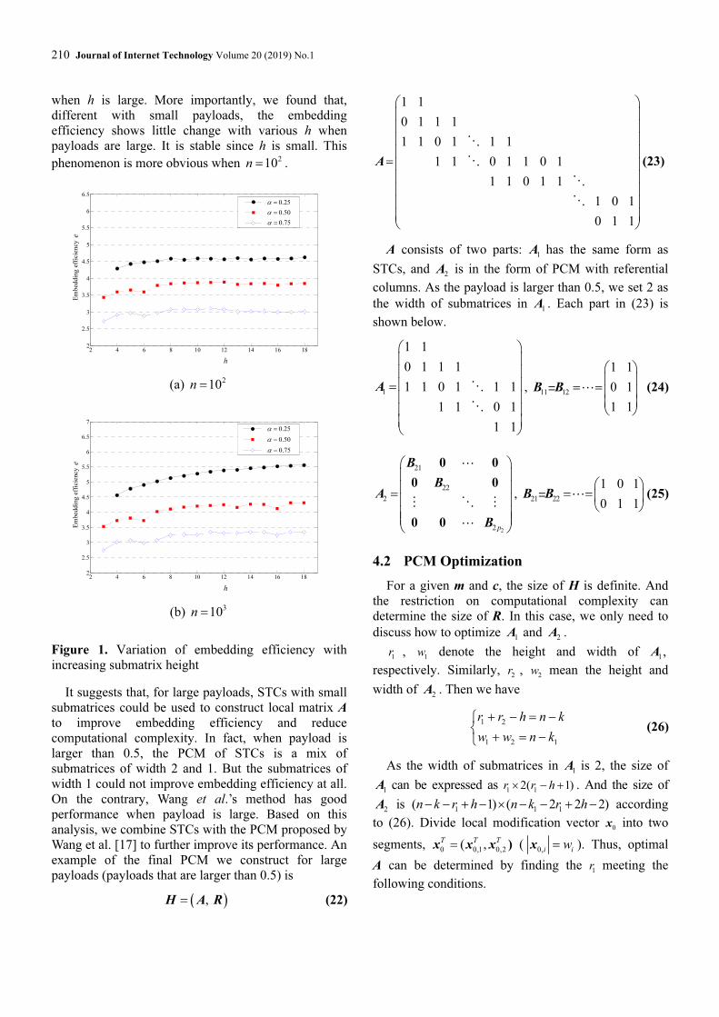
210 Journal of Internet Technology Volume 20 (2019) No.1
when h is large. More importantly, we found that,
different with small payloads, the embedding
efficiency shows little change with various h when
payloads are large. It is stable since h is small. This
phenomenon is more obvious when 210n = .
2 4 6 8 10 12 14 16 182
2.5
3
3.5
4
4.5
5
5.5
6
6.5
h
Em
bed
din
g e
ffic
iency
e
0.25α =
0.50α =
0.75α =
(a) 210n =
2 4 6 8 10 12 14 16 182
2.5
3
3.5
4
4.5
5
5.5
6
6.5
7
h
Em
bed
din
g e
ffic
iency
e
0.25α =
0.50α =
0.75α =
(b) 310n =
Figure 1. Variation of embedding efficiency with
increasing submatrix height
It suggests that, for large payloads, STCs with small
submatrices could be used to construct local matrix A
to improve embedding efficiency and reduce
computational complexity. In fact, when payload is
larger than 0.5, the PCM of STCs is a mix of
submatrices of width 2 and 1. But the submatrices of
width 1 could not improve embedding efficiency at all.
On the contrary, Wang et al.’s method has good
performance when payload is large. Based on this
analysis, we combine STCs with the PCM proposed by
Wang et al. [17] to further improve its performance. An
example of the final PCM we construct for large
payloads (payloads that are larger than 0.5) is
( ), =H A R (22)
1 1
0 1 1 1
1 1 0 1 1 1
1 1 0 1 1 0 1
1 1 0 1 1
1 0 1
0 1 1
⎛ ⎞⎜ ⎟⎜ ⎟⎜ ⎟⎜ ⎟
=⎜ ⎟⎜ ⎟⎜ ⎟⎜ ⎟⎜ ⎟⎝ ⎠
�
�
�
�
A (23)
A consists of two parts: 1
A has the same form as
STCs, and 2
A is in the form of PCM with referential
columns. As the payload is larger than 0.5, we set 2 as
the width of submatrices in 1
A . Each part in (23) is
shown below.
1
1 1
0 1 1 1
1 1 0 1 1 1
1 1 0 1
1 1
⎛ ⎞⎜ ⎟⎜ ⎟⎜ ⎟=⎜ ⎟⎜ ⎟⎜ ⎟⎝ ⎠
�
�
A , 11 12
1 1
0 1
1 1
⎛ ⎞⎜ ⎟
= =⎜ ⎟⎜ ⎟⎝ ⎠
�=B B
(24)
2
21
22
2
2p
⎛ ⎞⎜ ⎟⎜ ⎟=⎜ ⎟⎜ ⎟⎜ ⎟⎝ ⎠
0 0
0 0
0 0
�
� � �
�
B
BA
B
, 21 22
1 0 1
0 1 1
⎛ ⎞= =⎜ ⎟
⎝ ⎠�=B B (25)
4.2 PCM Optimization
For a given m and c, the size of H is definite. And
the restriction on computational complexity can
determine the size of R. In this case, we only need to
discuss how to optimize 1
A and 2
A .
1r ,
1w denote the height and width of
1,A
respectively. Similarly, 2r ,
2w mean the height and
width of 2
A . Then we have
1 2
1 2 1
r r h n k
w w n k
+ − = −⎧⎨
+ = −⎩ (26)
As the width of submatrices in 1
A is 2, the size of
1A can be expressed as
1 12( 1)r r h× − + . And the size of
2A is
1 1 1( 1) ( 2 2 2)n k r h n k r h− − + − × − − + − according
to (26). Divide local modification vector 0
x into two
segments, 0 0,1 0,2
( ,T T T= )x x x (
0,i iw=x ). Thus, optimal
A can be determined by finding the 1r meeting the
following conditions.

A Further Study of Optimal Matrix Construction for Matrix Embedding Steganography 211
1
0,1 0,2 1
1 1
2 2
2 1
2 1 1
arg min ( ) ( ) {0, 3, 4, , }
subject to 2
1
2 2 2
r
r n k
r n k
r w
r n k r h
w n k r h
ω ω⎧ + ∈ −⎪⎪ ≤ −⎪
≤⎨⎪ = − − + −⎪⎪ = − − + −⎩
�x x
(27)
The expectations of 0,1
( )ω x can be estimated
through experiments using STCs, the PCM dimension
of which is 1 1
( 1) 2( 1)r h r h− + × − + . The red line in
Figure 2 indicates 0,1
( ( ))E ω x when 3h = .
5 10 15 20 250
2
4
6
8
10
12
14
16
18
20
1A
0,1( ( ))E ω x
0,2( ( ))E ω x
0,1 0,2( ( ) ( ))E ω ω+x x
Figure 2. Variation of Hamming weight of the
modification vector with different 1r
2 2 1 11w r k k r h− = − − + − denotes the number of
submatrices in 2
A . According to (8), their heights are
1
1 1
1 1
1
1
1 1
1 1
1 1
1 1
1
( 1)
1( 2)
1
1
i
n k r hif i k k r h
k k r h
n k r ht
n k r hk k r h
k k r h
if i k k r h
⎧⎢ ⎥− − + −< − − + −⎪⎢ ⎥
− − + −⎣ ⎦⎪⎪ − − + − −⎪
= ⎨⎢ ⎥− − + −⎪ − − + − ⎢ ⎥⎪ − − + −⎣ ⎦⎪
⎪ = − − + −⎩
(28)
Furthermore, we can get the average number of
embedding changes using 2
A .
1 11 ( 1) 2
0,2 1 0
0
( 1) 2 1
0
( ( )) (
( 1))
i i
i
i
i i
ii
i
jk k r h t t
ti j k
tk
jt t
itj t k
tk
CE j
C
Ct j
C
ω
− − + − +⎢ ⎥⎣ ⎦
= =
=
= + +⎢ ⎥⎣ ⎦
=
= ⋅ +
⋅ − +
∑ ∑∑
∑∑
x
(29)
For 60n = , 36n k− = , 1
3k = , the average change
number using 2
A is shown by the blue line in Figure 2.
Taking 0,1
( ( ))E ω x and 0,2
( ( ))E ω x into consideration,
the optimal size of 1
A and 2
A can be determined as
20 36× and 18 21× on this occasion.
4.3 Computational Complexity Analysis
Searching for the coset leader of ( )CH
u with
respect to the proposed PCM for large payloads also
needs two steps. The computational complexity of
finding the coset leader corresponding to 2
A is linear
with 2
w . Therefore, the computational cost of the first
step is close to that of STCs, i.e., 1
( 2 )hO w . More
precisely, considering that extra computation is needed
at the juncture of two kinds of submatrices, the whole
computational complexity of our method is 1
1 1
1 2 ,(2 (2 2 (2 1) ))
k h h h
h tO w w ν
− −
⋅ ⋅ + + − ⋅ , where
1 11
,
1
min {1,2, , 1}
subject to 1
t
ii
h t t
ii
t i k k r h
t h
ν=
=
⎧ ∈ − − + −⎪= ⎨
≥ −⎪⎩
∑
∑
�
(30)
5 Experimental Results
If an ME method has low computational complexity,
larger PCM can be utilized and it may lead to higher
embedding efficiency. Therefore, some papers only
ensure that ME methods have the same computational
complexity and embedding rate, ignoring PCM sizes,
when compare embedding efficiency. But, in practice,
cover data may be divided into small parts and the
embedding process is performed on each part [9]. In
this case, comparing ME methods should under the
condition that PCMs have the same size. So we take
PCM sizes into consideration in the following
experiments.
5.1 Experiments of ME for Small Payloads
Experiment-1: Take the case of 60n = for example.
Following the searching process described in Section
3.2, we got the optimal PCMs for small payloads in
Table 1. For each payload, 5000 messages and 5000
covers are generated. All of them are random binary
sequences. Embed these messages and record
embedding efficiencies. Calculate the mean value of
5000 experimental results as the final result.
Comparison of embedding efficiency between
Hamming codes [14], Tian et al.’s method [1], Wang et
al.’s method [17] and the proposed method is shown in
Figure 3.

212 Journal of Internet Technology Volume 20 (2019) No.1
Table 1. Optimal PCM schemes with different message lengths ( 60n = )
n k− e r p 1k n k− e r p
1k
1 2.0000 {1} 1 59 16 4.2172 {1,3,4,4,4} 5 7
2 2.6667 {2} 1 57 17 4.0964 {2,3,4,4,4} 5 5
3 3.4286 {3} 1 53 18 3.9387 {3,3,4,4,4} 5 1
4 4.2667 {4} 1 35 19 3.7531 {1,3,3,4,4,4} 6 0
5 5.1613 {5} 1 29 20 3.8226 {3,3,3,3,4,4} 6 2
6 4.6875 {1,5} 2 28 21 3.7433 {2,2,3,3,3,4,4} 7 8
7 4.4700 {2,5} 2 26 22 3.7581 {3,3,3,3,3,3,4} 7 3
8 4.5508 {3,5} 2 22 23 3.6095 {1,3,3,3,3,3,3,4} 8 2
9 4.7974 {4,5} 2 14 24 3.4595 {2,3,3,3,3,3,3,4} 8 0
10 4.6153 {1,4,5} 3 13 25 3.5889 {1,3,3,3,3,3,3,3,3} 9 3
11 4.4571 {2,4,5} 3 11 26 3.3471 {2,3,3,3,3,3,3,3,3} 9 1
12 4.4412 {3,4,5} 3 7 27 3.2727 {1,2,3,3,3,3,3,3,3,3} 10 0
13 4.3189 {1,3,4,5} 4 6 28 3.1638 {1,2,2,2,3,3,3,3,3,3,3} 11 1
14 4.1691 {2,3,4,5} 4 4 29 3.0933 {1,1,2,2,2,3,3,3,3,3,3,3} 12 0
15 4.1026 {3,3,4,5} 4 0 30 3.0769 {2,2,2,2,2,2,3,3,3,3,3,3} 12 0
Figure 3. Comparison of embedding efficiency when 60n =
From Figure 3, we can learn that: (1) the proposed
ME method can support different embedding capacities,
while Hamming codes can only embed at most 5 bits
of secret messages; (2) In Tian et al.’s method, PCM is
made up of several submatrices and columns which are
obtained by executing the bit-wise XOR operation
between two columns in different submatrices. When
the number of extra columns is large, this method may
have a good effect. Therefore, rare points in Figure 3
are better than our method, such as 10n k− = ; (3)
However, Tian et al.’s method takes no account of the
combination of the extra columns and potentially can’t
make full use of all the cover data. Along with the
increase of embedding rate, the number of submatrices
has a tendency to increase, and the extra columns
become fewer. This is bad for Tian et al.’s method, but
more combinations of extra columns could be dealt
with in our method. As a result, the proposed method
performs better in this phase; (4) On the whole, the
proposed method has the highest embedding efficiency
among these four methods.
The computational complexities of Hamming codes
and Tian et al.’s method are both ( )O n , and Wang et
al.’s method in this experiment is 6( 2 )O n . For 60n = ,
actual computational costs of our method are shown in
Table 2. It can be concluded that the proposed method
has equal or lower computational complexity to that of
the previous three methods.
Table 2. Variation of computational complexity with different message lengths ( 60n = )
n k− 1 2 3 4 5 6 7 8 9 10
C 1 1 1 1 1 1
28
0
2i
i
C
=
∑ 1
26
0
2i
i
C
=
∑ 1
22
0
2i
i
C
=
∑ 1
14
0
2i
i
C
=
∑2
13
0
3i
i
C
=
∑
n k− 11 12 13 14 15 16 17 18 19 20
C
2
11
0
3i
i
C
=
∑
2
7
0
3i
i
C
=
∑
3
6
0
4i
i
C
=
∑
3
4
0
4i
i
C
=
∑ 4 4
7
0
5i
i
C
=
∑
4
5
0
5i
i
C
=
∑ 5 2⋅ 6 26 2⋅
n k− 21 22 23 24 25 26 27 28 29 30
C 3
7 2⋅ 3
7 2⋅ 2
8 2⋅ 8 39 2⋅ 9 2⋅ 10 11 2⋅ 12 12
Experiment-2: In order to further test the
performance of the proposed ME method, we apply it
to StegVoIP [2]. StegVoIP selected 18 LSBs to hide
secret messages from each G.723.1 (6.3kbits/s) speech
frame. Hence, there are altogether 72 bits in 4
neighbouring frames. We randomly choose 40 or 60
bits from them and take these bits as a unit to perform
embedding process. The speech files we used in this
experiment are selected from An4 database [21]. They
have different lengths. Half of the speech files are
A Further Study of Optimal Matrix Construction for Matrix Embedding Steganography 213
recorded by female speakers and half of them are
recorded by male speakers. The secret messages are
still binary sequences generated randomly.
Perceptual evaluation of speech quality (PESQ) is
proposed by ITU. It’s a widely used objective speech
quality assessment method. PESQ ranges from -0.5
(the worst) to 4.5 (the best). It can measure the
difference between the stego speech and the original
speech, so we use it to verify the validity of ME
methods. Calculate the mean PESQ of 1000 original
female speech files and 1000 original male speech files
separately. And compare them with PESQ of stego
speeches with different encoding methods. The results
are shown in Table 3. From Table 3, we can learn that:
PESQ of stego speeches using the proposed method are
very close to the original speeches and larger than
stego speeches corresponding to other methods,
indicating that our method can effectively ensure the
speech quality.
Table 3. Comparison of PESQ
Female ( 40n = ) Male ( 40n = ) Female ( 60n = ) Male ( 60n = )
Embedding rate 0.1 0.3 0.5 0.1 0.3 0.5 0.1 0.3 0.5 0.1 0.3 0.5
Original speech 3.769 3.769 3.769 3.776 3.776 3.776 3.769 3.769 3.769 3.776 3.776 3.776
Tian et al. 3.738 3.567 3.426 3.745 3.574 3.432 3.687 3.531 3.346 3.694 3.538 3.352
Wang et al. 3.684 3.534 3.399 3.691 3.540 3.404 3.617 3.425 3.267 3.623 3.432 3.275
Proposed method 3.738 3.575 3.426 3.745 3.581 3.433 3.715 3.532 3.346 3.722 3.540 3.352
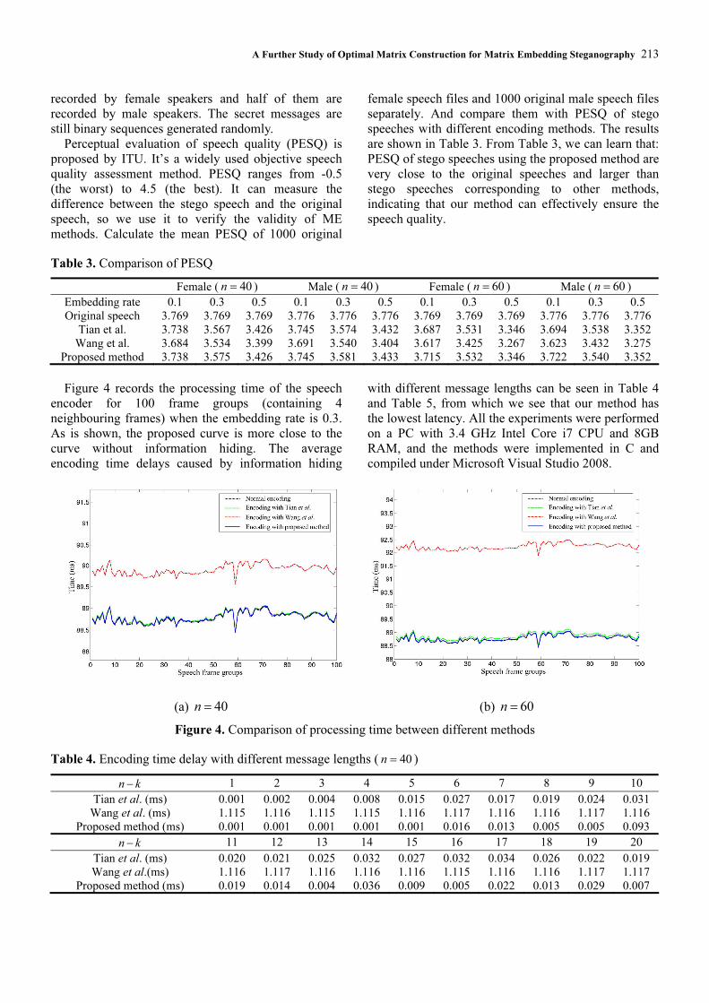
Figure 4 records the processing time of the speech
encoder for 100 frame groups (containing 4
neighbouring frames) when the embedding rate is 0.3.
As is shown, the proposed curve is more close to the
curve without information hiding. The average
encoding time delays caused by information hiding
with different message lengths can be seen in Table 4
and Table 5, from which we see that our method has
the lowest latency. All the experiments were performed
on a PC with 3.4 GHz Intel Core i7 CPU and 8GB
RAM, and the methods were implemented in C and
compiled under Microsoft Visual Studio 2008.
(a) 40n = (b) 60n =
Figure 4. Comparison of processing time between different methods
Table 4. Encoding time delay with different message lengths ( 40n = )
n k− 1 2 3 4 5 6 7 8 9 10
Tian et al. (ms) 0.001 0.002 0.004 0.008 0.015 0.027 0.017 0.019 0.024 0.031
Wang et al. (ms) 1.115 1.116 1.115 1.115 1.116 1.117 1.116 1.116 1.117 1.116
Proposed method (ms) 0.001 0.001 0.001 0.001 0.001 0.016 0.013 0.005 0.005 0.093
n k− 11 12 13 14 15 16 17 18 19 20
Tian et al. (ms) 0.020 0.021 0.025 0.032 0.027 0.032 0.034 0.026 0.022 0.019
Wang et al.(ms) 1.116 1.117 1.116 1.116 1.116 1.115 1.116 1.116 1.117 1.117
Proposed method (ms) 0.019 0.014 0.004 0.036 0.009 0.005 0.022 0.013 0.029 0.007

214 Journal of Internet Technology Volume 20 (2019) No.1
Table 5. Encoding time delay with different message lengths ( 60n = )
n k− 1 2 3 4 5 6 7 8 9 10
Tian et al. (ms) 0.001 0.002 0.004 0.008 0.015 0.041 0.046 0.035 0.032 0.034
Wang et al. (ms) 3.454 3.456 3.455 3.456 3.456 3.456 3.456 3.456 3.456 3.456
Proposed method (ms) 0.001 0.001 0.001 0.001 0.001 0.048 0.041 0.032 0.027 0.214
n k− 11 12 13 14 15 16 17 18 19 20
Tian et al. (ms) 0.048 0.052 0.059 0.067 0.056 0.064 0.053 0.055 0.058 0.043
Wang et al. (ms) 3.455 3.456 3.456 3.456 3.458 3.456 3.455 3.455 3.456 3.456
Proposed method (ms) 0.129 0.052 0.137 0.052 0.004 0.405 0.128 0.009 0.005 0.021
n k− 21 22 23 24 25 26 27 28 29 30
Tian et al. (ms) 0.055 0.052 0.049 0.043 0.062 0.057 0.043 0.045 0.031 0.028
Wang et al. (ms) 3.456 3.456 3.456 3.456 3.457 3.456 3.456 3.456 3.456 3.456
Proposed method (ms) 0.049 0.050 0.029 0.007 0.061 0.016 0.009 0.020 0.011 0.011
5.2 Experiments of ME for Large Payloads
Experiment-3: Embed messages into random cover
data using Fridrich et al.’s method [15] and the
proposed method for large payloads. The
computational complexity of Fridrich et al.’s method is
( 2 )kO n . When embedding rate is not large enough, the
ME time will be too long. So we set 60n = and the
minimum embedding rate is set to be 0.75. To ensure
that the proposed method can realize fast embedding,
the computational complexity of our method is limited
to be lower than 10(2 )O . Notice that, for a given cover
length and computational complexity, there are many
parameter combinations of h and k1 resulting in
different PCM. We select the parameters which can
yield the least distortion among them. For each payload,
we embed 5000 blocks of random messages, and
calculate the average embedding efficiency.
Experimental results are shown in Figure 5 and Table 6,
from which we can draw a conclusion that two ME
methods achieve almost equal embedding efficiency,
while the embedding speed of our method outperforms
Fridrich et al.’s method.
Figure 5. Comparison of embedding efficiency when 60n =
Table 6. Comparison of embedding speed between
Fridrich et al.’s method and the proposed method
( 60n = )
Embedding rate 0.75 0.80 0.85 0.90 0.95
Fridrich’s method
(Kbits/s) 0.05 0.53 6.06 64.13 804.52
Proposed method
(Kbits/s) 2.83 2.88 6.06 64.13 804.52
Fridrich et al.’s method is an exhaustive method. It
has the capability of searching global optimal solution
within the defined space. Different from this, the coset
leader we found using STCs or Wang et al.’s method is
a local optimal solution. The larger the number of
random columns in PCM is, the more combinations
will be considered in searching for the coset leader,
and thus a higher embedding efficiency we will get.
Therefore, local matrix R tends to be maximized
within the range of allowable computational
complexity. The computational complexity shoud be
lower than 10(2 )O in this experiment, so the number of
random columns is 10 at most. When the embedding
rate is larger than 0.85, the random columns needed by
PCM is less than 10. As a result, the PCMs we
constructed using the proposed method are the same as
Fridrich et al.’s method at this moment.
Experiment-4: Just like Experiment-2, we apply ME
to StegVoIP and make a comparison between the
proposed method and existing fast ME methods in [10]
and [17]. The computational complexity of Fridrich et
al.’s method is too high to be applied to VoIP
steganography. So we didn’t use it in this experiment.
For 60n = , 6(2 )C O≤ , we select the best parameters
(shown in Table 7) of the proposed method and get
their embedding efficiencies (shown in Figure 6(a)).
According to the conclusions of Experiment-3, the
proposed ME method are the same as Fridrich et al.’s
method when 54n k− ≥ . Therefore, it is not discussed
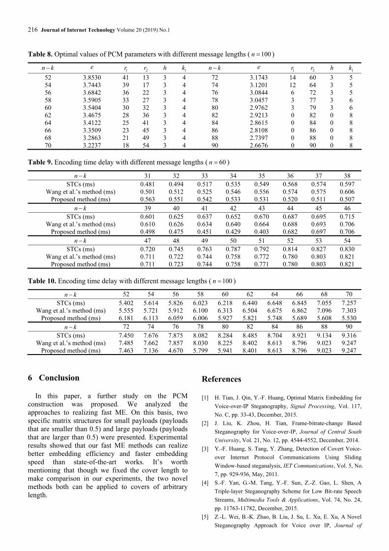
in this experiment. Similarly, Table 8 and Figure 6(b)
only show the results when 100,n = 8(2 ),C O≤
92.n k− ≤ Table 7 and Table 8 illustrate that the novel

A Further Study of Optimal Matrix Construction for Matrix Embedding Steganography 215
method turns into Wang et al.’s method when payload
is close to 1. Figure 7 records the processing time of
speech encoder with different ME methods in several
cases. And Table 9, Table 10 show the precise
encoding time delay caused by information hiding.
According to these results, we can see that a promising
embedding efficiency is obtained by the proposed
method while maintaining low computational
complexity.
(a) 60n = (b) 100n =
Figure 6. Comparison of embedding efficiency between different methods
(a) 60n = , 40n k− = (b) 100n = , 66n k− =
Figure 7. Comparison of processing time between different methods
Table 7. Optimal values of PCM parameters with different message lengths ( 60n = )
n k− e 1r
2r h 1
k n k− e 1r
2r h 1
k
31 3.7086 24 9 3 2 43 3.0146 8 37 3 2
32 3.6296 23 11 3 2 44 3.0418 0 44 0 6
33 3.5522 22 13 3 2 45 3.9763 0 45 0 6
34 3.4681 21 15 3 2 46 2.9407 0 46 0 6
35 3.4007 20 17 3 2 47 2.9385 0 47 0 6
36 3.3457 18 20 3 2 48 2.9136 0 48 0 6
37 3.3048 17 22 3 2 49 2.8602 0 49 0 6
38 3.2225 15 25 3 2 50 2.8257 0 50 0 6
39 3.1811 14 27 3 2 51 2.7749 0 51 0 6
40 3.1338 12 30 3 2 52 2.7129 0 52 0 6
41 3.0990 10 33 3 2 53 2.6447 0 53 0 6
42 3.0688 9 35 3 2 54 2.5793 0 54 0 6
216 Journal of Internet Technology Volume 20 (2019) No.1
Table 8. Optimal values of PCM parameters with different message lengths ( 100n = )
n k− e 1r
2r h 1
k n k− e 1r
2r h 1
k
52 3.8530 41 13 3 4 72 3.1743 14 60 3 5
54 3.7443 39 17 3 4 74 3.1201 12 64 3 5
56 3.6842 36 22 3 4 76 3.0844 6 72 3 5
58 3.5905 33 27 3 4 78 3.0457 3 77 3 6
60 3.5404 30 32 3 4 80 2.9762 3 79 3 6
62 3.4675 28 36 3 4 82 2.9213 0 82 0 8
64 3.4122 25 41 3 4 84 2.8615 0 84 0 8
66 3.3509 23 45 3 4 86 2.8108 0 86 0 8
68 3.2863 21 49 3 4 88 2.7397 0 88 0 8
70 3.2237 18 54 3 4 90 2.6676 0 90 0 8
Table 9. Encoding time delay with different message lengths ( 60n = )
n k− 31 32 33 34 35 36 37 38
STCs (ms) 0.481 0.494 0.517 0.535 0.549 0.568 0.574 0.597
Wang et al.’s method (ms) 0.501 0.512 0.525 0.546 0.556 0.574 0.575 0.606
Proposed method (ms) 0.563 0.551 0.542 0.533 0.531 0.520 0.511 0.507
n k− 39 40 41 42 43 44 45 46
STCs (ms) 0.601 0.625 0.637 0.652 0.670 0.687 0.695 0.715
Wang et al.’s method (ms) 0.610 0.626 0.634 0.640 0.664 0.688 0.693 0.706
Proposed method (ms) 0.498 0.475 0.451 0.429 0.403 0.682 0.697 0.706
n k− 47 48 49 50 51 52 53 54
STCs (ms) 0.720 0.745 0.763 0.787 0.792 0.814 0.827 0.830
Wang et al.’s method (ms) 0.711 0.722 0.744 0.758 0.772 0.780 0.803 0.821
Proposed method (ms) 0.711 0.723 0.744 0.758 0.771 0.780 0.803 0.821
Table 10. Encoding time delay with different message lengths ( 100n = )
n k− 52 54 56 58 60 62 64 66 68 70
STCs (ms) 5.402 5.614 5.826 6.023 6.218 6.440 6.648 6.845 7.055 7.257
Wang et al.’s method (ms) 5.555 5.721 5.912 6.100 6.313 6.504 6.675 6.862 7.096 7.303
Proposed method (ms) 6.181 6.113 6.059 6.006 5.927 5.821 5.748 5.689 5.608 5.530
n k− 72 74 76 78 80 82 84 86 88 90
STCs (ms) 7.450 7.676 7.875 8.082 8.284 8.485 8.704 8.921 9.134 9.316
Wang et al.’s method (ms) 7.485 7.662 7.857 8.030 8.225 8.402 8.613 8.796 9.023 9.247
Proposed method (ms) 7.463 7.136 4.670 5.799 5.941 8.401 8.613 8.796 9.023 9.247
6 Conclusion
In this paper, a further study on the PCM
construction was proposed. We analyzed the
approaches to realizing fast ME. On this basis, two
specific matrix structures for small payloads (payloads
that are smaller than 0.5) and large payloads (payloads
that are larger than 0.5) were presented. Experimental
results showed that our fast ME methods can realize
better embedding efficiency and faster embedding
speed than state-of-the-art works. It’s worth
mentioning that though we fixed the cover length to
make comparison in our experiments, the two novel
methods both can be applied to covers of arbitrary
length.
References
[1] H. Tian, J. Qin, Y.-F. Huang, Optimal Matrix Embedding for
Voice-over-IP Steganography, Signal Processing, Vol. 117,
No. C, pp. 33-43, December, 2015.
[2] J. Liu, K. Zhou, H. Tian, Frame-bitrate-change Based
Steganography for Voice-over-IP, Journal of Central South
University, Vol. 21, No. 12, pp. 4544-4552, December, 2014.
[3] Y.-F. Huang, S. Tang, Y. Zhang, Detection of Covert Voice-
over Internet Protocol Communications Using Sliding
Window-based steganalysis, IET Communications, Vol. 5, No.
7, pp. 929-936, May, 2011.
[4] S.-F. Yan, G.-M. Tang, Y.-F. Sun, Z.-Z. Gao, L. Shen, A
Triple-layer Steganography Scheme for Low Bit-rate Speech
Streams, Multimedia Tools & Applications, Vol. 74, No. 24,
pp. 11763-11782, December, 2015.
[5] Z.-L. Wei, B.-K. Zhao, B. Liu, J. Su, L. Xu, E. Xu, A Novel
Steganography Approach for Voice over IP, Journal of

A Further Study of Optimal Matrix Construction for Matrix Embedding Steganography 217
Ambient Intelligence & Humanized Computing, Vol. 5, No. 4,
pp. 601-610, August, 2014.
[6] R. Crandall, Some Notes on Steganography, http://www.dia.
unisa.it/~ads/corso-security/www/CORSO-0203/steganografia/
LINKS%20LOCALI/matrix-encoding.pdf.
[7] J. Fridrich, P. Lisoněk, D. Soukal, On Steganographic
Embedding Efficiency, 8th Inernational Workshop on
Information Hiding, Alexandria, VA, 2006, pp. 282-296.
[8] J. Fridrich, T. Filler, Practical Methods for Minimizing
Embedding Impact in Steganography, Security,
Steganography and Watermarking of Multimedia Contents IX,
Bellingham, WA, 2007, pp. 201-215.
[9] T. Filler, J. Judas, J. Fridrich, Minimizing Embedding Impact
in Steganography Using Trellis-coded Quantization, Media
Forensics and Security II, Bellingham, WA, 2010, pp. 175-
178.
[10] T. Filler, J. Judas, J. Fridrich, Minimizing Additive Distortion
in Steganography Using Syndrome-trellis Codes, IEEE
Transactions on Information Forensics and Security, Vol. 6,
No. 3, pp. 920-935, September, 2011.
[11] J. Qin, H. Tian, Y.-F. Huang, J. Liu, Y. Chen, T. Wang, Y.
Cai, X. A. Wang, An Efficient VoIP Steganography Based on
Random Binary Matrix, 10th International Conference on
P2P, Parallel, Grid, Cloud and Internet Computing, Krakow,
Poland, 2015, pp. 462-465.
[12] Z.-J. Wu, H.-J. Gao, D.-Z. Li. An Approach of
Steganography in G.729 Bitstream Based on Matrix Coding
and Interleaving, Chinese Journal of Electronics, Vol. 24, No.
1, pp. 157-165, January, 2015.
[13] X.-L. Li, S.-R. Cai, W.-M. Zhang, B. Yang, A Further Study
of Large Payloads Matrix Embedding, Information Sciences,
Vol. 324, No. C, pp. 257-269, December, 2015.
[14] A. Westfeld, F5–A Steganographic Algorithm: High Capacity
Despite better Steganalysis, 4th Intermational Workshop on
Information Hiding, Pittsburgh, PA, 2001, pp. 289-302.
[15] J. Fridrich, D. Soukal, Matrix Embedding for Large Payloads,
IEEE Transactions on Information Forensics and Security,
Vol. 1, No. 3, pp. 390-395, September, 2006.
[16] Q. Mao, A Fast Algorithm for Matrix Embedding
Steganography, Digital Signal Processing, Vol. 25, No. 1, pp.
248-254, February, 2014.
[17] C. Wang, W.-M. Zhang, J.-F. Liu, N. Yu, Fast Matrix
Embedding by Matrix Extending, IEEE Transactions on
Information Forensics and Security, Vol. 7, No. 1, pp. 346-
350, February, 2012.
[18] Y.-K. Gao, X.-L. Li, T.-Y. Zeng, B. Yang, Improving
Embedding Efficiency via Matrix Embedding: A Case Study,
16th IEEE International Conference on Image Processing,
Cairo, Egypt, 2009, pp. 109-112.
[19] J.-J. Wang, H.-S. Chen, A Suboptimal Embedding Algorithm
with Low Complexity for Binary Data Hiding, IEEE
International Conference on Acoustics, Speech and Signal
Processing, Kyoto, Japan, 2012, pp. 1789-1792.
[20] J.-J. Wang, C.-Y. Lin, H.-S. Chen, T.-Y. Yang, A Suboptimal
Embedding Algorithm for Binary Matrix Embedding,
International Symposium on Computer, Consumer and
Control, Taichung, Taiwan, 2012, pp. 165-168.
[21] An4 Database, http://www.speech.cs.cmu.edu/databa-
ses/an4/.
Biographies
Zhanzhan Gao received the B.S.
degree in electronic science and M.S.
degree in information security from
Zhengzhou information science and
technology institute in 2011 and 2014,
respectively. He is now pursuing the
Ph.D. degree in information security.
His research interests include information hiding and
multimedia processing.
Guangming Tang received the B.S.,
M.S. and Ph.D. degrees in information
security from Zhengzhou information
science and technology institute in
1983, 1990, and 2008. She is now a
professor at Department of Information
Security, Zhengzhou information
science and technology institute. Her research interests
include information hiding and cryptography.

218 Journal of Internet Technology Volume 20 (2019) No.1
Recommended


