A Flexible Model of Term‐Structure Dynamics of Commodity Prices: A
Comparative Analysis with a Two‐Factor Gaussian Model
Hiroaki Suenaga
School of Economics and Finance, Curtin University, GPO Box U1987, Perth, WA 6845,
AUSTRALIA.
Email: [email protected]
Abstract
This study compares two approaches to modeling a term structure of commodity prices. The
first approach specifies the stochastic process of the underlying spot price and derives from
the stipulated spot price dynamics valuation formulas of futures and other derivative
contracts through no arbitrage. The second approach, as introduced by Smith (2005), is to
model the dynamics of the entire futures curve directly by a set of common stochastic factors
and to specify factor loadings by flexible functions of time‐to‐maturity and contract delivery
month. Empirical applications of the models to four commodities (gold, crude oil, natural gas,
and corn) reveal that the volatility of futures prices exhibits more complex dynamics than the
pattern implied by the model stipulating a two‐factor Gaussian process of the underlying
spot price. Specifically, the flexible model of futures returns depicts the maturity effect and,
particularly for the three consumption commodities, strong seasonal and cross‐sectional
variations in variance and covariances of concurrently traded contracts. Incorporating the
depicted variance and covariance dynamics leads the flexible model of futures returns to
suggest hedging strategies that are more effective than the strategies based on the
conventional two‐factor term‐structure model.
Keywords: commodity prices, term‐structure model, volatility, hedging

1
1. Introduction
Recent increase in the level and volatility of oil, metals, and other primary commodity
prices has created tremendous uncertainties for producers, consumers, and other traders of
these commodities. Volatility of commodity prices also affects the national economy, both
directly by altering revenue and expenditure on these commodities and indirectly by
deferring new investments. In such circumstances, a better understanding of the stochastic
properties of these commodity prices and tools to hedge against price risks becomes
increasingly important for the smooth functioning of the commodity supply chain.
Stochastic dynamics of commodity prices and valuation of derivative contracts have long
been studied in the field of financial economics. The standard approach in this literature is to
specify the stochastic process of the underlying asset, usually the spot price of the commodity
under investigation, and derive from the stipulated process valuation formulas of futures and
other derivative contracts whose payoff depends on the value of the underlying asset realized
at the contract maturity date (see Hull, 2002). This approach dates back to Black and Scholes
(1973) who derived pricing formulas of European options under the assumption that the
underlying asset value (stock price) follows a geometric Brownian motion (GBM). While
following the same approach, many studies modeling commodity price dynamics commonly
specify one of the underlying stochastic factors to follow a mean‐reverting (MR) process
because, for many consumption commodities, demand and/or supply response forces
unusually high or low prices to revert to the long‐run equilibrium level (Schwartz, 1997).
Recent advances in this modeling approach have been attained through increasing the
number of common stochastic factors and/or stipulating an increasingly complex stochastic
process of each latent factor.1 These flexible models generally exhibit a better fit to the
observed price data while maintaining the model parsimonious with pricing formulas of
derivative contracts typically determined by a small number of parameters characterizing the
stochastic dynamics of the underlying factors. However, it is often understated that the
benefit of a parsimonious specification is gained at the cost of potentially large errors in
approximating true stochastic dynamics of commodity prices. It has been widely
acknowledged that, unlike stocks and other conventional financial assets, commodity prices
exhibit complex dynamics. The theory of storage (e.g., Williams and Wright, 1991; Routledge
et al., 2000) illustrate that, for a commodity with a significant storage cost, inter‐temporal
1 Lautier (2005) provides a comprehensive review on applications of term‐structure models to various
commodities.

2
arbitrage establishes an equilibrium constellation of spot and futures prices along which the
marginal benefit of current consumption is equal to or above the expected marginal benefit of
storing a commodity for future consumption. The weak inequality stems from a non‐
negativity of physical storage. If supply is ample relative to demand, inter‐temporal arbitrage
induces positive inventory up to a point where the two prices differ by the cost of carry. In
this case, the convenience yield, representing the implicit revenue from holding a physical
asset, is close to zero. In contrast, when supply is scarce, discretionary inventory is driven to
zero and the marginal benefit of current consumption exceeds the marginal benefit of future
consumption due to high convenience yield. In this case, speculative storage plays a minor
role in price determination and the inter‐temporal price linkage breaks. This discontinuity in
the inter‐temporal price link means that price correlations across concurrently traded
contracts vary by season. Many commodities also exhibit pronounced seasonality in price and
volatility, reflecting seasonality in the underlying demand and/or supply. Volatility tends to
be high in the period of tight demand‐supply balance because market shocks of even a small
magnitude can cause a large price swing. It is also expected that volatility is inversely related
to inventory because demand and supply shocks can be absorbed through adjusting
inventory. Stochastic processes of the spot price and other underlying factors stipulated in
many models of commodity price dynamics, even recently developed complex models, are
often too simple to induce a futures price formula that replicates the complex dynamics of
commodity futures prices implied by the theory of storage.
An alternative approach to modeling a term structure of commodity prices, as recently
introduced by Smith (2005) and later extended by Suenaga and Smith (2011), is to model
directly the dynamics of futures curve. In this model, daily futures returns is decomposed
into a set of common stochastic factors affecting all futures returns and an idiosyncratic term.
By modeling futures returns rather than a price level, the model does not specify seasonal or
other deterministic variation in the underlying spot price. This model also avoids specifying
stochastic dynamics of the underlying factors and imposes no a priori restriction on the factor
loadings that connect underlying factors to observed futures returns. Rather, the model
specifies factor loadings and the variance of the idiosyncratic term directly by flexible
functions so that they can replicate highly non‐linear price dynamics of commodities with
significant storage costs and seasonality in demand or supply.
In this study, I compare the two approaches to the modeling of term structure of
commodity prices; one specifying directly the dynamics of daily futures returns as a flexible
function of common stochastic factors, and the other specifying the stochastic process of the

3
underlying spot price. I apply the two models to futures price data from four commodity
markets (crude oil, natural gas, gold, and corn). Results from this empirical analysis illustrate
that the volatility of daily futures prices exhibits highly non‐linear dynamics that cannot be
induced by the stochastic process of the underlying spot price stipulated in the conventional
two‐factor term‐structure model. Specifically, the flexible model of futures returns depicts a
maturity effect and, particularly for the three consumption commodities, strong seasonality in
both its levels and compositions among the two common stochastic factors and the
idiosyncratic error. These features together create substantial seasonal and cross‐sectional
variation in the price correlations of concurrently traded contracts. Incorporating the depicted
dynamics of price volatility and cross‐contract correlations allows the flexible model of
futures returns to suggest hedging strategies that are more effective than a strategy based on
the conventional term‐structure model specifying a two‐factor Gaussian process for the
underlying spot price.
The next section presents the two approaches to modeling a term structure of commodity
prices. The section also presents a composite model in which the factor loadings are specified
as in the conventional spot price‐based approach, yet allows for a flexible variance structure
of the idiosyncratic errors. Section 3 reports results from estimating the three models
empirically with unbalanced panel data from four commodity markets. The results are
compared across the models with an emphasis on seasonal and cross‐sectional variations in
the depicted price variance and cross‐contract correlations. Section 4 considers the
implication of the models for an optimal strategy to hedge price risk. Section 5 provides a
synopsis of the findings to conclude the paper.
2. Comparison of Two Modeling Approaches for Term‐Structure of
Commodity Futures
This section presents a flexible model of futures curve dynamics in which daily futures
returns is decomposed into a set of common latent factors and an idiosyncratic term. This
model is then compared with the conventional term‐structure model specifying stochastic
dynamics of the underlying spot price and deriving pricing formulas of futures and other
derivative contracts.
2.1. A flexible model of commodity futures returns
One approach to modeling commodity price dynamics, as introduced by Smith (2005)
and later extended by Suenaga and Smith (2011), is to model directly the daily price changes

4
of all concurrently traded futures contracts.2 In this approach, a daily return of futures
contract is decomposed into the common latent factors and an idiosyncratic term. The model
incorporates time varying conditional heteroskedasticity of latent factors and time and cross‐
sectional variation in the factor loadings and idiosyncratic variances.
The model with two common factors is expressed in the following form,
(1) , 1 1 1, 2 2 2, 3 3 ,
ln ( , )( ) ( , )( ) ( , )( )m t t t m tF m d m d m d u
where , , , 1
ln ln lnm t m t m tF F F is the change from t to 1t of the log price of the futures
contract that matures at m. 1,t and
2,t are the latent factors that affect all contracts traded on
t, with E[ ] 0tε and
2E[ ]
t tI ε ε t and E[ ] 0
t s ε ε for t s where 1, 2,
( )t t t
ε . ,m t
u is the
idiosyncratic error. It is assumed that ,
E[ ] 0m tu and
,V[ ] 1
m tu m and t,
, ,E[ ] 0
m s m tu u
s t , and, , ,
E[ ] 0n t m tu u m n . In other words,
,m tu represents shocks that are specific to
the contract maturing at m and uncorrelated serially and across concurrently traded contracts.
1( , )m d and
2( , )m d are the factor loadings determining the extent to which common shocks,
1,t and
2,t , are reflected in the price change of the contract maturing at m, and
3( , )m d
determines the standard deviation of the shock specific to the contract maturing at m. In
model (1), three coefficients i
are included to allow for a potentially non‐zero deterministic
change in the log futures price. They are multiplied by the associated ( , )im d function so
that they are interpreted as representing the forward premium associated with the two
common factors (i = 1, 2) and idiosyncratic error (i = 3).3
The three terms, ( , )im d for i = 1, 2, and 3, are specified as deterministic functions of
contract delivery month (m) and time to delivery of the contract ( d m t ),
(2) , ,0 , ,1 , ,2 , ,2 11 max max
2 2( , ) exp sin cos
K
i i m i m i m k i m kk
kd kdm d a a d a a
d d
2 The model as originally introduced by Smith (2005) is named as the Partially Overlapping Time‐Series
or “POTS” model for it is developed for the analysis of commodity futures return data, which usually
forms a partially overlapping time series or an unbalanced panel. In this paper, I refer to the model
defined in (1)‐(3) as a “flexible model of futures returns” or simply “flexible model” because the other
two models examined in this paper are also applied to partially overlapping time‐series data. 3 The estimates of the three coefficients
i are very small for all four commodities examined in this
paper. Restricting these coefficients equal to zero does not alter the results presented in Sections 3 and 4.

5
where maxd is the maximum days to maturity for which the model is estimated. Specification
(2) allows the three terms ( , )im d to be a flexible function of time‐to‐maturity (d) and permits
this function to vary by contract delivery month (m). The combination of m and d uniquely
identifies a trade date (t) in the year through d m t . Thus, specification (2) also captures
seasonal variation in the factor loadings and the idiosyncratic variance. The function, ( , )im d ,
becomes more flexible with the number of trigonometric terms (K). Although this extra
flexibility allows a better fit to the observed data, it also makes the model more sensitive to
extreme observations. In the empirical estimation of the model in Section 3, I set K = 3 so that
the model is flexible enough to capture seasonality and maturity effects while avoiding excess
sensibility to extreme observations.
The unconditional variance of daily log futures returns is given by
3 2
, 1V[ ln ] ( , )
m t iiF m d
. Thus, the model can replicate potentially very complex dynamics
in the variance of log futures returns and its composition among the three components.
Furthermore, the two latent factors affect all contract prices whereas the idiosyncratic errors
are uncorrelated across contracts. Therefore, correlations across concurrently traded contracts
are determined by the share of the variance attributable to the two common factors.
Specification (2) allows these cross‐contract correlations to vary by season and across
contracts.
For identification, the constraint is imposed as 2 , ,0 2 , ,2 1 2 , ,1 max1
10K
m m k mka a a d
so that
2 max( , ) 0m d for all m. That is, the loading of the second factor is close to zero at the
maximum days to maturity. The condition is equivalent to the one used in Schwartz and
Smith (2000), which allows the two factors to be interpreted as representing the long‐term
(LT) and short‐term (ST) factor, respectively.4
The conditional variance of latent factors tε is specified by a bivariate GARCH(1,1)
model in a diagonal BEKK specification (Engle and Kroner, 1985),
(3) 1E[ | ]t
t t t
ε ε H
1
1 1 1E[ | ]t
t t t t
H Ω βH β α ε ε α
4 In the two‐factor model of Schwartz and Smith (2000), the loading of the short‐term factor in the
futures price equation is given by exp() where and represents the mean‐reversion coefficient and
time‐to‐maturity, respectively. The value of this loading decreases exponentially and converges to zero
with , given > 0. The two‐factor model of Sorensen (2002) reviewed in Section 2.2 shares this property.
6
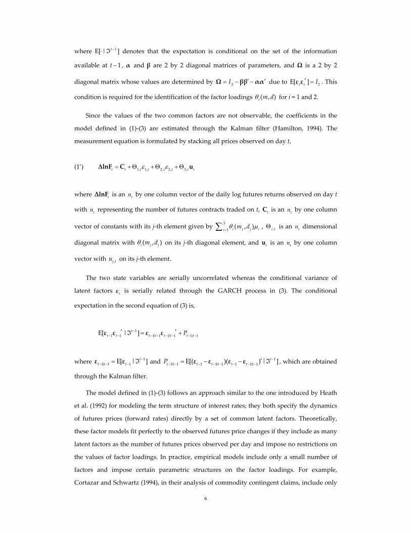
where 1E[ | ]t denotes that the expectation is conditional on the set of the information
available at 1t , α and β are 2 by 2 diagonal matrices of parameters, and Ω is a 2 by 2
diagonal matrix whose values are determined by 2I Ω ββ αα due to
2E[ ]
t tI ε ε . This
condition is required for the identification of the factor loadings ( , )im d for i = 1 and 2.
Since the values of the two common factors are not observable, the coefficients in the
model defined in (1)‐(3) are estimated through the Kalman filter (Hamilton, 1994). The
measurement equation is formulated by stacking all prices observed on day t,
(1’) 1, 1, 2, 2, 3,t t t t t t t t ΔlnF C u
where t
ΔlnF is an tn by one column vector of the daily log futures returns observed on day t
with tn representing the number of futures contracts traded on t,
tC is an
tn by one column
vector of constants with its j‐th element given by 3
1( , )i j j iim d
, ,i t
is an tn dimensional
diagonal matrix with ( , )i j jm d on its j‐th diagonal element, and
tu is an
tn by one column
vector with ,j tu on its j‐th element.
The two state variables are serially uncorrelated whereas the conditional variance of
latent factors tε is serially related through the GARCH process in (3). The conditional
expectation in the second equation of (3) is,
1
1 1 1| 1 1| 1 1| 1E[ | ]t
t t t t t t t tP
ε ε ε ε
where 1
1| 1 1E[ | ]t
t t t
ε ε and 1
1| 1 1 1| 1 1 1| 1E[( )( ) | ]t
t t t t t t t tP
ε ε ε ε , which are obtained
through the Kalman filter.
The model defined in (1)‐(3) follows an approach similar to the one introduced by Heath
et al. (1992) for modeling the term structure of interest rates; they both specify the dynamics
of futures prices (forward rates) directly by a set of common latent factors. Theoretically,
these factor models fit perfectly to the observed futures price changes if they include as many
latent factors as the number of futures prices observed per day and impose no restrictions on
the values of factor loadings. In practice, empirical models include only a small number of
factors and impose certain parametric structures on the factor loadings. For example,
Cortazar and Schwartz (1994), in their analysis of commodity contingent claims, include only

7
three factors and plot the factor loadings as a function of time‐to‐maturity only. These
restrictions create a discrepancy between the model’s implied and observed price movement.
Previous studies often do not model explicitly this residual component. The model defined in
(1)‐(3) differs from Cortazar and Schwartz (1994) in these regards; it specifies the two factor
loadings as flexible parametric functions of time‐to‐maturity and contract delivery month. It
also models parametrically the idiosyncratic error with its variance also specified by a flexible
function. These specifications together allow the model to depict complex seasonal and cross‐
sectional variations in the variance and covariances of concurrently traded contract prices.
2.2. A conventional two‐factor term‐structure model of commodity prices
A conventional approach to modeling the term structure of commodity prices is to
specify the stochastic processes of the spot price of the commodity and to derive from the
stipulated spot price dynamics pricing formulas of futures and other derivative contracts. For
example, the following two‐factor Gaussian model is commonly considered for the analysis
of various commodities with seasonality in demand and/or supply,5
(4)
ln ( )t t t
t x x
t t z z
x z
S f t x z
dx dt dw
dz z dt dw
dw dw dt
where tS is the spot price at period t, f(t) is the seasonal mean price that is a deterministic
function of time, tx and
tz are the state variables representing, respectively, the long‐term
(LT) and short‐term (ST) deviation from the seasonal mean price, x
dw and z
dw are the
increment to the standard Brownian motion that are correlated through x z
dw dw dt , and
, , x
, and z
are parameters determining, respectively, drift rate, mean reversion rate,
and diffusion rate of the two stochastic factors.
The price in period t of the futures contract that matures at T is obtained as the period t
conditional expectation, under the risk neutral probability measure, of the spot price at T. It
5 Model (4) has been considered, for example, for the analysis of electricity (Lucia and Schwartz, 2002),
natural gas (Manoliu and Tompaidis, 2002), and agricultural commodity futures, such as corn, wheat,
and soybean (Sorensen, 2002). Gibson and Schwartz (1990) and Nielsen and Schwartz (2004) also
consider a two‐factor model in analyzing oil and copper, yet they parameterize the dynamics of two
factors differently from (4) so that the two factors are interpreted as representing spot price and
convenience yield factor. Schwartz and Smith (2000) show that these models are identical to model (4)
aside from the absence of seasonal variation in mean price.

8
can be shown that, for the spot price following the process (4), the price of this futures
contract is obtained as,6
(5) ln ( , ) ( ) ( )t t
F t T f T A x z e
where2 2 2(1 ) ( )(1 )
( )2 4x z x z z
x
e eA
, T t is the time‐to‐
maturity, and two coefficients x and z
represent the market prices of risk associated with
the corresponding stochastic factor.
The set of parameters defining model (4), { , , , , , }x z x z
, is usually estimated
with futures price data. To fit equation (5) into multiple prices with different maturity dates
observed per day, an error term is added to the right‐hand side of (5), which makes the values
of the two factors x and z unidentifiable. Thus, the model is commonly estimated with a
filtering method. In state‐space form, the model is presented as,
(6) ,
ln ( , ) ( ) ( ) i
ii i i t t T tF t T f T A x z e u … Measurement equation
(7) 1 1,
1 2,
t t t
t t t
z e z v
x x v
… Transition equation
where iT is the maturity date of i‐th contract ( 1,...,
ti n ) observed on day t,
1, 2 ,( )
t t tv vv is
serially uncorrelated and identically distributed with ~ N(0, )tv H and H is the symmetric
matrix with 2
x and 2
z on the main diagonal and
x z off diagonal. In (6),
,T tu is the
measurement error representing errors in reporting prices or factors affecting futures prices
that are not accounted for by the two common factors. It is commonly assumed that
,E[ ] 0
T tu ,t T ,
1 2, ,E[ ] 0
T s T tu u for s t and/or
1 2T T . Thus, econometrically,
,T tu
represents the idiosyncratic error that is uncorrelated serially and contemporaneously across
contracts. It is also commonly assumed that 2
,V[ ]
T t Tu t. That is, the variance is allowed to
vary by the contract maturity date (T) but not by trade date (t) or time‐to‐maturity (T t ).
6 Futures price formula (5) assumes constant market prices of risk. See, for example, Sorensen (2002) for
details.

9
2.3. Model comparison
A major difference between conventional term‐structure models of commodity prices and
the flexible model of futures returns defined in (1)‐(3) is that the former specifies the
dynamics of price level whereas the latter specifies the dynamics of price return. By modeling
price returns rather than level, the flexible model does not specify seasonality and other
deterministic variations in the underlying spot price that result from demand/supply
seasonality and other characteristics of the underlying commodity.7 Thus, the model is free
from bias in specifying such deterministic price variation.
To compare the two models in further detail, take the first difference of the futures price
formula in (7),
(8) , , , 1 2, 1, ,ln ln ln ( )
T t T t T t t t T tF F F B v e v u
where 2 2 2
2( ) (1 ) (1 )2 4
z x z x zx
eB e e e
and 2
,~ N(0,2 )iid
T t Tu
because , , , 1T t T t T t
u u u and 2
,~ N(0, )iid
T t Tu t.
Comparison of (8) and (1) reveals three major benefits of the flexible model over the
conventional approach in modeling a term structure of commodity prices with the specified
spot price dynamics. First, model (1) specifies the factor loadings by flexible functions for
both the LT and ST factors. In contrast, the factor loadings are determined by a small number
of parameters defining the stochastic dynamics of the underlying state variables in
conventional term‐structure models. Specifically, for the two‐factor model (8), the loadings of
the ST factor decrease exponentially with time‐to‐maturity at an identical rate for all
contracts, whereas those of the LT factor are constant at unity for all contracts throughout the
trading horizon. Second, the flexible model (1) specifies the variance of the idiosyncratic error
by a flexible function of time‐to‐maturity and allows this function to vary across contract
delivery months. In contrast, conventional term‐structure models impose a simplistic
structure on the variance of the measurement error ,T t
u with the variance allowed to vary
only by the delivery month of contract but not by time‐to‐maturity. Third, the innovations to
7 These deterministic price variations correspond to the seasonal mean price and deterministic trend
(denoted as f(T) and ) in the conventional term‐structure model (6). First differencing eliminates these
terms and leaves only the innovation errors (1v and
2v ) on the right‐hand side of (8). The stochastic
dynamics of the two state variables still remain in (8), yet only implicitly by restricting functional forms
of the factor loadings.

10
the state variables, ,i tv (i = 1, 2), are specified to follow a bivariate GARCH process in the
flexible model (1) while they are assumed homoskedastic in the conventional term‐structure
model (8).
Strong restrictions imposed on the stochastic dynamics of the underlying factors and the
variance of the measurement error potentially lead conventional term‐structure models to
draw an erroneous portrait of price volatility of a storable commodity with demand and/or
supply seasonality. In particular, the model in (6) and (8) stipulates that the variance
attributable to the two common factors increases exponentially as the contract approaches
maturity whereas the variance of the measurement error does not vary with time‐to‐
maturity. 8 Consequently, the model implies that correlation across concurrently traded
contracts decreases monotonically with time‐to‐maturity. By contrast, the flexible model
defined in (1)‐(3) allows for the magnitude of futures price change resulting from the
common market shocks and that resulting from contract specific shocks to differ both by
time‐to‐maturity and by contract delivery date. This flexibility allows the model to replicate
highly non‐linear dynamics of commodity prices expected by the theory of storage. The
model also gives the same flexibility to the variance structure of the two common factors and
that of the idiosyncratic error and thus avoids the magnitude and dynamics of the cross‐
contract correlation to be determined by the model specification.
In the next section, I estimate the flexible model of futures returns with empirical data
from the four markets and compare its estimation results with the estimate of the two
alternative models. The first model is the conventional two‐factor model defined in (5)‐(7). I
estimate the subset of the model parameters that appear on the model’s first difference form
(8), which is directly comparable to the flexible model. Since first differencing eliminates the
deterministic variation in mean price level and deterministic variations in the two common
factors, the comparison signifies the adequacy of the parsimonious specifications imposed in
the conventional two‐factor model on the stochastic dynamics of the underlying factors (as
determinants of the factor loadings) and the variance of the measurement error. The second
alternative model is the composite model in which factor loadings are specified as in the
conventional two‐factor model (hence imposing a restrictive specification on the stochastic
dynamics of the latent factors), whereas the variance of the measurement error is specified by
a flexible function as in (2). That is,
8 In other words, of the three components comprising the daily futures returns in model (8), the ST
factor is only the component that can vary by time‐to‐maturity, and the measurement error is only the
component that allows variation across contracts with different maturity dates.

11
(9) , 2, 1, 3 ,ln ( ) ( , )
T t t t T tF B v e v m d u
where 3( , )m d is as defined in (2). This model nests the two‐factor model in (4)‐(7). It is
expected that the flexible specification of the variance of measurement error captures complex
volatility dynamics, albeit partially.
3. Data and Estimation
This section empirically estimates the three models reviewed in Section 2 with the
unbalanced panel data from four commodity markets. The section starts with the description
of the data examined and then reports results from estimating the three models with
emphasis on their implied volatility dynamics.
3.1. Data
The three models presented in Section 2 are estimated with the data from the markets for
the following four commodities with varying characteristics:
Natural gas – consumption good with strong seasonality in demand,
Corn – consumption good with strong seasonality in supply,
Crude oil – consumption good with very weak seasonality in demand and supply, and
Gold – investment good with virtually no seasonality either in demand or supply.
The models are estimated using data on daily settlement prices of futures contracts
traded at the New York Mercantile Exchange (crude oil, natural gas, and gold) and Chicago
Board of Trade (corn). The data analysed in this paper are from the period between 1984/1/1
and 2007/12/31 for corn and gold, 1984/4/1 and 2007/12/31 for crude oil, and 1991/4/1 and
2007/12/31 for natural gas. For each contract, daily prices to the last trading day of the
contract are used for analysis.9 Since long‐dated contracts do not trade actively, contracts of
more than twelve months to maturity are excluded from the analysis, except that contracts up
to eighteen months to maturity are analyzed for corn.10 Excluding these observations leaves
9 Crude oil and natural gas contracts cease trading before the delivery month whereas corn and gold,
contracts trade into the delivery month. See exchange’s website (www.cmegroup.com) for details in
contract specifications. 10 Corn exhibits strong supply seasonality with harvest usually arriving around September to early
November. The theory of storage suggests that inter‐temporal price link breaks at the end of crop year,
creating potentially very complex price dynamics for the September (and December) contract at around

12
70,800 prices among 307 contracts for crude oil, 52,780 prices among 223 contracts for natural
gas, 43,820 prices among 168 contracts for gold, and 48,762 prices among 142 contracts for
corn.
All three models are estimated by the method of maximum likelihood with the likelihood
obtained through the Kalman filter as described in Section 2. I first estimate the conventional
two‐factor model (8) which is the most parsimonious of the three models. The composite
model (9) differs from model (8) only in the specification of the variance of the measurement
error. The model is estimated with the starting values of the coefficient vector 3a in
3 3( , ; )m d a obtained by minimizing the sum of the squared differences between 2
3 3( , ; )m d a
and the squared residuals from the estimated model (8). Finally, for the flexible model (1), I
obtaine the starting values in two steps: (i) calculate the variance attributable to each of the
three components (LT and ST factor, and the idiosyncratic error) from the estimated
composite model and (ii) find the values of each coefficient vector ia ( 1,...,3i ) that
minimize the sum of the squared differences between ( , ; )i im d a and the predicted values of
the corresponding component in the composite model calculated in step (i). Robustness is
checked by estimating the model with different sets of starting values obtained by
distributing fraction of the variance of the idiosyncratic error from the estimated composite
model to the other two components in step (i) of the above two‐step procedure.
3.2. Estimation results: Model specification
Table 1 summarizes the results from the specification test. It shows that, for all four
commodities considered, the flexible model of futures returns is preferred to the other two
models, and the composite model is preferred to the conventional two‐factor model
according to both the Akaike and Schwarz Information Criteria. The results provide strong
evidence that the conventional two‐factor model stipulating restrictive structures on the
factor loadings and the variance of the measurement errors is not supported empirically for
all four commodities. Surprisingly, the model is not supported even for gold for which the
storage cost is not significant and virtually no demand or supply seasonality exists.
12 months before maturity. I analyze the contracts as far as eighteen months to maturity to capture
potentially very interesting price movements of these two contracts in this period.

13
3.3. Estimation results: Flexible model
Figures 1 through 4 illustrate the results of estimating the flexible model of futures
returns for the four commodities. These figures plot, for each contract delivery month: (a) the
estimated loadings of the LT factor, (b) the loadings of the ST factor, (c) the standard
deviation of the idiosyncratic shocks, and (d) the share of the total variance accounted for by
the two common factors, which are all aligned by trade date. These components are
calculated as ,
ˆ( , ; )i i mm d a for the first three components (i = 1, 2, and 3, respectively for
component (a), (b), and (c)) and 2 32 2
, ,1 1ˆ ˆ( , ; ) / ( , ; )
i i m i i mi im d m d
a a for the last component,
where , , ,0 , ,2
ˆ ˆ ˆ{ ,..., }i m i m i m K
a aa is the vector of coefficients estimated for each of the three
components (i = 1, 2, 3), each delivery month (m), and for each of the four commodities.11
(a) Natural gas
In panel (a) of figure 1, the loadings of the LT factor estimated for natural gas indicate
two notable features. First, for all twelve contracts, the estimated factor loadings increase as
the contract approaches the maturity date. Second, the factor loadings in the last few months
of trading are substantially higher for the contracts maturing in winter than those maturing in
summer. The loadings of the ST factor exhibit the same features, but in greater magnitude
than those observed for the LT factor (panel b). In addition, for all twelve contracts, the
loadings of the ST factor start increasing rapidly in May, before which they are virtually zero
for all twelve contracts. In panel (c) of figure 1, the variance of the idiosyncratic error,
particularly that for winter contracts, increases very rapidly as the contract approaches
maturity. This indicates that high volatility in the last one month of trading, commonly
referred as the maturity effect, represents market shocks that are specific to each contact and
are of a very short‐term nature. Unlike the two common factors, the idiosyncratic errors are
not contemporaneously correlated across concurrently traded contracts. Thus, a rapid
increase in the variance of the idiosyncratic errors implies that correlation between nearby
and distant futures contracts decreases rapidly over the winter season (panel d).
These estimates of the factor loadings and the variance of the idiosyncratic error in the
estimated flexible model are consistent with the price dynamics implied by the theory of
storage for natural gas. In the flexible model (1), the total variance of log futures price change
is given by 3 2
,1ˆ( , ; )
i i mim d
a at d days before the contract maturing in the month m. Thus,
11 The denominator in the formula for component (d) represents the total variance, owning to the
assumption that two latent factors and idiosyncratic errors are uncorrelated one another.

14
high factor loadings and high variance of the idiosyncratic errors translate to high volatility of
winter contracts in the last few months of trading. During this peak‐demand period, tight
demand‐supply imbalance causes demand or supply shock of even a small magnitude to
follow a large price swing, which cannot be absorbed through adjusting inventory because
the inventory is effectively zero at the end of the demand season. Low inventory also means
that the inter‐temporal price linkage breaks at the end of the winter peak‐demand season
because, in any normal year, no physical stock is carried over from late winter (when price
peaks) to early spring (when price is the lowest). The estimated flexible model reflects this
feature with a large share of price variation accounted for by the ST factor and the
idiosyncratic error for the December through March contracts in their last few months of
trading. During the same period, the loadings of the ST factor and the variance of the
idiosyncratic error stays very low for contracts maturing in May and thereafter.
[Insert figure 1 somewhere here]
(b) Corn
In figure 2, the estimated flexible model reveals complex volatility dynamics for corn. The
depicted volatility pattern differs from natural gas, yet it is characterized by seasonality in the
supply of the underlying commodity. In this figure, the loadings of both the LT and ST factor
start increasing for all five contracts around April and peaks in July to August (panels a and
b). This observation implies that large price fluctuations of contract prices during this period
are highly correlated across the five contracts maturing in the post‐harvest season. High price
volatility during this period reflects the arrival of important information. In particular, corn
crops in the U.S. are typically planted in early April through June and harvested later in the
year, usually from September to early November. The date and yield of harvest are
determined by weather conditions during summer. Thus, the contracts maturing post‐harvest
exhibit large price fluctuations and high cross‐contract price correlation during this period.
Volatility starts decreasing in mid‐summer after most weather conditions are revealed and
reaches the lowest point when actual harvesting is realized around October. Over these
periods, prices move very closely for five contracts maturing post‐harvest, because corn is an
annual crop and one harvest in the current year needs to be stored for consumption until the
new harvest arrives in the subsequent year. In normal years, the current harvest is fully
consumed during the demand season and no inventory is carried over to the post‐harvest
season. Thus, the contracts maturing post‐harvest show minimal price movement before

15
these crops are planted in early spring. Panel (c) of figure 2 indicates that much of high
volatility in the last one month of trading originates in the contract specific errors. The
variance of the idiosyncratic error is particularly high for the July contract. This is
conveniently explained by low inventory at the end of the demand year, which does not
allow unexpected demand and/or supply shocks to be absorbed through inventory
adjustment. High variance of contract‐specific shock means that a small share of variance is
accounted for by the two common factors. This share and, consequently, the correlation
among concurrently traded contracts decrease rapidly in the last one month of the trading
period, particularly for the July contract (panel d).
[Insert figure 2 somewhere here]
(c) Crude oil
Crude oil is generally thought to have much weaker demand seasonality than natural
gas. However, the estimated flexible model indicates moderate seasonality and maturity
effects for the volatility of crude oil price (figure 3). In panel a of figure 3, the estimated
loadings of the LT factor is slightly higher for all twelve contracts during winter months. The
volatility also increases for all twelve contracts in the last two months of trading, and
volatility in this period is slightly higher for winter (January and February) and summer (July
and August) contracts. Much of this high volatility in the last two months of trading is
captured by the ST factor and the idiosyncratic errors (panels b and c), indicating that this
high volatility is caused by shocks that are not persistent and have little impact on the prices
of distant maturity contracts. The variance of the idiosyncratic error increases rapidly in the
last month of trading and is particularly high for the January and two summer contracts,
causing substantial declines in correlation between these contracts and other concurrently
traded contracts (panel d).
[Insert figure 3 somewhere here]
(d) Gold
In figure 4, the estimated flexible model shows virtually no seasonality or maturity effect
for gold price volatility. For all six contracts, the estimated loadings of the LT factor are
slightly higher from October to March, yet this seasonal difference is negligible, with
16
variation ranging no more than 3.5 percent of the average (panel a). Another feature that
differentiates gold from the other three commodities is that the estimated loadings of the ST
factor and the variance of the idiosyncratic errors are very small for all contracts; they are on
average 5.7 percent and 1.7 percent, respectively, of the estimated loadings of the LT factor.
These results imply that much of the price shocks to the gold markets are of a long‐term
nature. High persistence of price shocks is as expected because gold is traded primarily for
investment rather than consumption and, unlike other exhaustible resources, the amount of
its deposits is well known. Due to large loadings of the LT factor, relative to the variance of
the idiosyncratic error, the two common factors account for a large share of the total variance,
resulting in high cross‐contract correlation for gold as seen in panel (d) of figure 4.
[Insert figure 4 somewhere here]
3.4. Estimation results: Conventional two‐factor model
Figures 5 through 8 present the results of estimating the conventional two‐factor model in
the first difference form (8) for the four commodities. These figures plot, for each contract: (a)
the variance of futures price attributable to the two common factors, which is calculated as
ˆ ˆ2 2 2 ˆˆ ˆ ˆ ˆx z x z
e e , (b) the variance of the idiosyncratic error 2
,ˆu m
, and (c) the share of
the variance accounted for by the two common factors as calculated by
ˆ ˆ2 2 2 2 2 1
, ,ˆˆ ˆ ˆ ˆ ˆ ˆ1 ( )
u m x z x z u me e . In panel a of figures 5 through 8, the variance
attributable to the two common factors increases exponentially as the contract approaches
maturity for all four commodities. This property, as discussed in Section 2, is the direct result
of the model specification that the LT and ST factors follow the GBM and MR processes,
respectively.
[Insert figure 5 somewhere here]
The conventional model allows the variance of the idiosyncratic error to vary by contract
delivery date but not by time‐to‐maturity. In panel b of figure 5, the model estimated for
natural gas indicates a higher variance of the idiosyncratic error for winter (January through
March) contracts than for the other contracts. However, the estimated variance of the
idiosyncratic error, even for these winter contracts, is negligible in size, when compared to
the variance attributable to the two common factors. These estimates cause the model to

17
imply very high cross‐contract correlation, which increases as contracts approach maturity
because the variance attributable to the ST factor increases exponentially. These implications
for the magnitude of cross‐contract correlation and its dynamics over time‐to‐maturity are
exactly opposite to the implications of the flexible model.
These results signify the severity of the restrictions imposed by the specifications of the
conventional two‐factor model. Of the three stochastic components in the right‐hand side of
the model in (8), the ST factor is the only component that captures the dynamics of the price
variance over the trading horizon, yet it only allows the variance to decrease exponentially
with time‐to‐maturity at an identical rate for all contracts. It neither permits non‐monotonic
change of the price variance nor allows the variance to change at different rates across
contracts. The model also restricts the idiosyncratic error, ,T t
u , to be the only component to
capture the cross‐contract difference in price variance. The estimation results described above
are determined by these specifications of the model. For natural gas, the model allocates a
large share of the price variance to the ST factor to capture strong maturity effects. It implies
low variance of the idiosyncratic errors because seasonal variation in the volatility of natural
gas price is small relative to the maturity effect. The severity of these restrictions is apparent
when the model is compared with the flexible model, in which the three components are
equally flexible in their seasonal and cross‐sectional variation and the composition of the
observed price movements among the three components is determined by cross‐contract
price correlation.
In figures 6 through 8, the conventional two‐factor model estimated for corn, crude oil,
and gold exhibits the same results as for natural gas. For all three commodities, the variance
attributable to the two common factors decreases gradually with time‐to‐maturity at the
identical rate for all contracts. The variance of the idiosyncratic error exhibits cross‐contract
variation, with variance slightly higher for the July corn contract, the August gold contract,
and the winter crude oil contracts. However, for all three commodities and for all contracts,
the variance of the idiosyncratic error is constant over the trading horizon and much smaller
than the variance attributable to the two common factors. The results imply that the two
common factors account for a large share of price variance and that this share increases as the
contract approaches maturity; the implications are exactly opposite to the estimated flexible
models. For gold only, the difference between the flexible model and the conventional two‐
factor model is small because very weak seasonality and maturity effects lead both models to
assign a dominant share of the price variance to the LT factor, resulting in very small loadings
of the ST factor and a small variance of the idiosyncratic error.
18
[Insert figures 6‐8 somewhere here]
3.5. Estimation results: Composite model
Figures 9 through 12 show the results from estimating the composite model (9).12 In
figure 9, the variance attributable to the two common factors for natural gas exhibits the same
dynamic pattern but is slightly smaller in magnitude than the estimate in the conventional
two‐factor model (panel a). In panel (b), the variance of the idiosyncratic error estimated for
the composite model is substantially greater than the estimates for the conventional two‐
factor model and exhibits strong seasonality and maturity effect. Strong seasonality and
maturity effect of the idiosyncratic error is reflected in the total variance, resulting in a
dynamics similar to the one estimated for the flexible model. Nonetheless, the share of the
total variance accounted for by the two common factors exhibits different dynamics between
the two models simply because the compositions of the price variance among the three
components differ between the two models (see figure 9.c and figure 1.d).
[Insert figure 9 somewhere here]
Figures 10 through 12 show that the composite model estimated for corn, crude oil, and
gold yields results similar to those for natural gas. The variance attributable to the two
common factors decreases with time‐to‐maturity yet at a slower rate than in the conventional
two‐factor model. On the other hand, the variance of the idiosyncratic error is estimated
substantially greater for the composite model than for the conventional two‐factor model. The
variance estimate for the composite model also exhibits strong maturity effects with variance
in the last month of trading being particularly large for the July contract for corn and the
January, July, and August contracts for crude oil. The maturity effect captured by the
idiosyncratic error dominates the increase in the loadings of the ST factor, implying that
cross‐contract correlation decreases rapidly in the last few months of trading. The increase in
the variance of the idiosyncratic error near the maturity date is much smaller for gold,
resulting in only a marginal reduction in the cross‐contract correlation near the maturity
dates.
12 In these figures, the variance of futures price attributable to the two common factors is calculated in
the same way as for the conventional two‐factor model whereas the variance attributable to the
idiosyncratic error is given as 2
3 3,ˆ( , ; )
mm d a .

19
[Insert figures 10‐12 somewhere here]
In summary, estimates of the flexible model of futures returns reveal that the volatility of
the three commodity futures; natural gas, corn, and crude oil, exhibit strong seasonality and
maturity effects. For natural gas, the volatility in the last few months of trading is particularly
high in winter months when demand peaks and inventory is low. Much of the high volatility
during this period is captured by the ST factor and the idiosyncratic error because low
inventory breaks the inter‐temporal price link, resulting in low cross‐contract price
correlation. For corn, volatility increases in spring through early summer when crops are
planted and as much of the weather shocks affecting the growth of these crops are revealed.
During this period, contracts maturing in the post‐harvest season exhibit high price
correlation. In the same period, the July contract that matures before harvest is subject to high
contract‐specific shock because low inventory at the end of the demand season breaks the
inter‐temporal price link. Crude oil exhibits high price volatility both in winter and summer
months, but the seasonality is moderate relative to natural gas and corn.
The conventional two‐factor model fails to capture these complex volatility dynamics of
the three consumption commodities because of strong restrictions imposed on the factor
loadings and the variance of the idiosyncratic error. In particular, the model allows neither a
cross‐contract nor a seasonal variation in the factor loadings. Neither does it allow a variation
in the variance of the idiosyncratic error by time‐to‐maturity. Consequently, the model
captures cross‐contract variation in the price volatility solely by the idiosyncratic error and
the maturity effect by the ST factor only. Flexible specification of the variance of the
idiosyncratic error permits the composite model to alleviate, albeit imperfectly, the
restrictions imposed in the conventional two‐factor model. The model replicates reasonably
well the complex volatility dynamics of the consumption commodities, yet it implies the
dynamics of cross‐contract correlations that are substantially different from the pattern
implied by the flexible model.
4. Implications for Optimal Hedging Strategy
In the previous section, estimates of the factor loadings and the variance of the
idiosyncratic errors differ substantially across three models. This section compares the three
models by their implications for an optimal hedging strategy.

20
4.1. Optimal hedging
I consider a trader with a spot position, Q, in period t, who simultaneously takes a short
position in X futures contracts for delivery at t . At t k , the trader clears its position
by selling Q units in the spot market and buying X futures contracts for delivery at .
Returns to this trader’s portfolio from t to t k is
, ,ln ln ln ln
t k t k t k t k t kW S Q F X S F Q
where lnt kS and
,ln
t kF are, respectively, the change from t to t k of the log spot price
and log price of futures contract for delivery at and 1XQ is the hedge ratio. The
variance of portfolio return is
2 2
, ,V[ ] V[ ln ] V[ ln ] 2 cov[ ln , ln ]
t k t k t k t k t kW Q S F S F
which is minimized when the hedge ratio is set as
(10) ,*
,
cov[ ln , ln ]
V[ ln ]
t k t k
t k
S F
F
The minimum variance attained by this hedge ratio is
(11) * 2 2
,V[ | ] V[ ln ](1 )
t k t k t kW S Q
where ,t k is the correlation between the change in the log spot price and the change in log
price of the futures contract for delivery at over the period between t and t k .
In the above variance minimization problem, the delivery date of the futures contract
included into the portfolio is taken as exogenous. In many organized exchanges, however,
multiple contracts with different maturity dates are traded simultaneously. Thus, the hedger
can choose from these multiple contracts one that attains the minimum portfolio variance.
Equation (11) indicates that, given the time of entry (t) and hedging horizon (k), the portfolio
variance is minimized when it includes the contract that exhibits the highest correlation with
the spot price over the hedging horizon. Once this contract is identified, the optimal hedge

21
ratio is determined according to (10) as the ratio of the covariance between the spot and
futures returns to the variance of futures returns.
4.2. Optimal hedging strategy according to the three models
It is apparent in (10) and (11) that specifications of variance and covariance dynamics of
spot and futures prices play an important role in determining the optimal hedging strategy.
Given the time of entry (t) and hedging horizon (k), one can calculate the optimal hedge ratio
() and the associated portfolio variance for every possible choice of futures contract included
into the portfolio (), based on the three models of daily futures returns estimated in Section
3. In particular, the variance of log futures returns in the denominator of the expression (10) is
calculated as
(12)
ˆ ˆ2 2 2 2
2 2 2
, 1 1 2 2 3 3
ˆ ˆ2 2 2 2
3 3
ˆˆ ˆ ˆ ˆ ˆ2 for conventional two‐factor model
ˆ ˆ ˆV[ ln ] ( , ; ) ( , ; ) ( , ; ) for flexible model
ˆ ˆˆ ˆ ˆ ˆ2 ( , ; ) for composite model
d d
x z x z
t
d d
x z x z
e e
F d d d
e e d
a a a
a
where d t is the time to delivery of the contract maturing at . Similarly, using the
nearby futures price as the proxy for the spot price,13 one can calculate the covariance
between the log returns to spot (nearby futures) and futures contract for delivery at as
(13)
0 0ˆ ˆ( ) ˆ2 2
,
1 0 0 1 1 1
2 0 0 2 2 2
ˆˆ ˆ ˆ ˆ ( ) for conventional two‐factor
and composite modelcov[ ln , ln ]
ˆ ˆ( , ; ) ( , ; )
ˆ ˆ( , ; ) ( , ; ) for flexible model
d d d d
x z x z
t t
e e e
S Fd d
d d
a a
a a
where 0 0d t and
0 is the delivery date of the nearby contract.
The first expression in (13) indicates that, for the conventional two‐factor model and the
composite model, the covariance between the log spot and log futures returns declines
monotonically with time‐to‐maturity (d) of the futures contract, which results from the
specification that the two common factors follow the GBM and MR processes in (4).
Furthermore, for the conventional two‐factor model, the variance of log futures returns also
declines monotonically with time‐to‐maturity in (12) yet at a slower pace than the decline in
the covariance of the spot and futures returns. Thus, the correlation between the two prices
13 This approximation is justified by the standard arbitrage argument that the price of the futures
contract converges to the spot price as the contract approaches the maturity date (see, for example, Hull,
2002).

22
declines monotonically with time‐to‐maturity and the model proposes that the hedger should
include into the portfolio the contract that is the closest to maturity to minimize the portfolio
variance. This implication for the optimal hedging strategy generally applies to the composite
model except that the model suggests the use of a more distant contract when the close‐to‐
maturity contracts are increasingly subject to high idiosyncratic variance 3 3
ˆ( , ; )d a (in which
case, the variance of the futures contract increases faster than the covariance between the two
prices). For the flexible model, the estimated factor loadings (1 1
ˆ( , ; )d a and 2 2
ˆ( , ; )d a ) and
the standard deviation of the idiosyncratic error (3 3
ˆ( , ; )d a ) exhibit substantial seasonal and
cross‐contract variations. Because the resulting spot‐futures correlations also exhibit seasonal
and cross‐sectional variations, the model proposes potentially very complex hedging
strategies that require both the size () and position () in the futures market to be adjusted
frequently across seasons.
Using the variance and covariance implied by each of the three models, I calculate the
optimal hedge ratio for a one‐day hedging horizon (k = 1) and t ranging from the first day to
the last day of a calendar year.14 For each t, I compare among the futures contracts maturing
in the subsequent twelve months by their correlation with the spot price and calculate the
optimal hedge ratio for the portfolio including the contract that exhibits the highest
correlation with the spot price.
Figure 13 illustrates, for each of the four commodities and for each of the three models,
how the futures contract included into the optimal portfolio shifts by the date of entry. The
figure shows that the optimal contract differs substantially among the three models. In the
figure, the optimal hedging strategy based on the conventional two‐factor model includes the
second position contract which is the closest to maturity after the nearby contract. This result
is expected because the model stipulates that, for each contract, the share of the variance
accounted for by the two common factors increases as the contract approaches its maturity
date. Thus, on any particular day, the contract closer to maturity exhibits a higher correlation
with the spot price unless it receives an exceptionally large idiosyncratic error. The exception
is observed for corn in July through mid‐August, during which the nearby (September)
14 I consider a hedging horizon of a single day because, in the absence of transaction cost for adjusting
futures position, the best (variance‐minimizing) strategy for a longer hedging horizon is to alter the
choice of contract () and the hedge ratio () every day so as to follow the optimal strategy for a one‐day
horizon. Staying with the previous‐day position could be optimal in the presence of transaction cost.
The best strategy in such a setting will depend on various factors such as the length of the hedging
horizon, the size of the transaction cost, and the risk aversion coefficient of the hedger. This is beyond
the scope of the paper and hence is left for future research.

23
contract exhibits higher correlation with the third position (March) contract than with the
second position (December) contract because of the high idiosyncratic variance of the latter.
[Insert figure 13 somewhere here]
The flexible model and composite model also suggest the use of the near‐to‐maturity
(second position) contract to hedge against the spot price risk for gold and corn. For crude oil
and natural gas, the two models suggest the use of a more distant contract; typically the third
position contract for crude oil and the third or fourth position contract for natural gas. The
two models suggest the use of distant contracts because the contracts closer to maturity are
subject to high idiosyncratic shocks and hence exhibit low correlation with the nearby
contract. For natural gas, the optimal portfolio includes the June or July contract early in the
calendar year (February to May). During this time, contracts for earlier maturity are subject to
high idiosyncratic shocks because low inventory at the end of the demand year disconnects
the inter‐temporal price links. The optimal contract shifts gradually from June to mid‐August
and, after that, it switches to a winter (December or January) contract. In this post summer
season, winter contracts are subject to little idiosyncratic shocks and much of their price
movements reflect common market shocks. Around the beginning of November, winter
contracts start receiving idiosyncratic shocks and the optimal contract is replaced with a more
distant contract.
Figure 14 plots the optimal hedge ratio against the time of entry for each of four
commodities. In panel (c), the optimal hedge ratio for gold is close to one throughout the year
for all three models. For gold, the variance of the idiosyncratic error is very small and a large
share of the price variance is accounted for by the LT factor in all three models. Thus, cross‐
contract correlation is very high and the variance and covariance in expression (10) are about
the same magnitude, resulting in the optimal hedge ratio of close to one. Similarly, the
optimal hedge ratio for corn remains close to one in panel (d), yet it is slightly lower for the
flexible model than for the other two models because the model implies higher idiosyncratic
error (and hence the lower covariance of the two prices) than the other two models.
[Insert figure 14 somewhere here]
For the other two commodities, the optimal hedge ratio differs substantially across the
three models. For both natural gas and crude oil, the optimal hedge ratio suggested by the

24
conventional two‐factor model shows little seasonal variation while it increases gradually
towards the end of each calendar month. The model stipulates that the variance attributable
to the two common factors increases exponentially as the contract approaches its maturity
date. The specification follows that the covariance between spot and futures return increases
faster than the variance of futures return, resulting in a gradual increase in the optimal hedge
ratio.
The composite model implies a similar strategy as the conventional two‐factor model for
hedging crude oil price risk, except that it suggests a much smaller variation of the optimal
hedge ratio within each month. In contrast, the strategy based on the flexible model indicates
a large increase in the optimal hedge ratio within each month simply because the estimated
factor loadings increase much faster in this model than in the other two models. For natural
gas, the optimal hedge ratio suggested by the flexible and composite model exhibits
substantial seasonal variation, reflecting the seasonal variation in the position of the futures
contract included in the optimal portfolio. In general, the optimal hedge ratio is high when
the portfolio includes a distant contract, because a distant contract is subject to little
idiosyncratic volatility and hence results in a low variance of futures return in the
denominator of (10). An optimal hedge ratio substantially above unity is often suggested
because the futures contract included in the portfolio exhibits small variation, a dominant
share of which represents common market shocks.
Table 2 presents the sum of the portfolio variance over a one‐year hedging horizon
expressed as the ratio to the variance of log spot price without hedging.15 In the table, all three
hedging strategies reduce portfolio variance dramatically. The three strategies are particularly
effective in reducing spot price risk for gold, for which cross‐contract correlation is
particularly high throughout the year. Portfolio variance is relatively high for crude oil and
natural gas, ranging from around 18 to 26 percent of the variance of the spot price. Hedging
15 These numbers are calculated under the assumption that the futures returns follow the process as
specified in the estimated flexible model, which receives the strongest empirical support for all four
commodities. Specifically, the variance of optimal portfolio is calculated, for each of the three hedging
strategies and for each entry date (t), as
* *
* 2 *
1 1 1( ), 1 ( ), 1V[ ( )] V[ ln ] ( ) V[ ln ] 2 ( )cov[ ln , ln ]
t t tt t t tW t S t F t S F
where * ( )t and * ( )t are
the delivery month of the futures contract included into the portfolio and the hedge ratio according to
the optimal strategy as seen in figures 13 and 14, respectively, and the variance and covariance are
evaluated according to the estimated flexible model, i.e., 3 2
1 0 01ˆV[ ln ] ( , ; )
t i iiS d
a ,
*
3 2 * *
1( ), 1ˆV[ ln ] ( ( ), ( ); )
i iit tF t d t
a , and *
2 * *
1 0 01( ), 1ˆ ˆcov[ ln , ln ] ( , ; ) ( ( ), ( ); )
t i i i iit tS F d t d t
a a
where * *( ) ( )d t t t .

25
strategies are less effective for these two commodities because the nearby contract is subject
to a large contract‐specific shock near maturity.
For all four commodities, portfolio variance is the smallest for a strategy based on the
flexible model. The composite model performs better than the conventional model in hedging
spot price risks for crude oil and natural gas. However, the strategy results in a substantially
greater portfolio variance than the strategy based on the flexible model for natural gas. This
result signifies the importance of specifying factor loadings by a flexible functional form to
properly account for not only seasonal and temporal variation in the price variance but also
the variation in the cross‐contract correlation, the latter of which plays a significant role in
designing an effective hedging strategy.
5. Conclusion
In this study, I compare a conventional two‐factor term‐structure model of commodity
futures with an alternative modeling approach of specifying variance of daily futures returns
directly by flexible functions. Empirical estimation of the flexible model of futures returns
with daily futures price data from four commodity markets reveal that the price volatility
exhibits strong maturity effects for three consumption commodities (crude oil, natural gas
and corn) and significant seasonal variation for commodities with strong seasonality in
demand (natural gas) or supply (corn). The futures price volatility for three consumption
commodities also exhibits complex dynamics in its composition among the two common
factors and the contract‐specific shock; volatility increases rapidly in the last month of
trading, a large share of which emanates from the contract‐specific shock. Consequently, the
correlation between nearby futures price and prices of more distant contracts declines sharply
as the contract approaches its maturity date. The model also reveals that the inter‐temporal
price linkage breaks at the end of winter for natural gas and at around September to early
November for corn. The finding supports the implication of the theory of storage that the
inter‐temporal price link breaks when inventory clears out, which happens at the end of
winter peak‐demand season for natural gas and in September right before the new harvest
arrives for corn.
The conventional two‐factor Gaussian model cannot replicate these complex price
dynamics due to restrictive specifications stipulated for the stochastic processes of the
underlying factors and the variance of the measurement error. In particular, the commonly
considered model specification forces the short‐term factor to capture entirely the variation in

26
the futures price volatility by time‐to‐maturity while it assigns the measurement error to
capture the seasonal and cross‐contract variation in the futures price volatility. The
specification also stipulates that the variance attributable to the two common factors
decreases exponentially with time‐to‐maturity at an identical rate for all contracts. Due to
these restrictions, the model implies that cross‐contract correlation increases monotonically as
the contract approaches maturity, which is exactly opposite to the implication of the flexible
model.
The composite model, allowing a flexible variance structure of the idiosyncratic error,
performs reasonably well in replicating the complex price dynamics depicted by the flexible
model. The results highlight that specifying a flexible variance structure of the idiosyncratic
error alone can improve the ability of conventional term‐structure models to replicate the
complex volatility dynamics of consumption commodities. These findings caution against a
recent trend in the development of term‐structure models, which focuses exclusively on
adopting more flexible stochastic processes of common stochastic factors while maintaining
restrictive structures on the variance of the measurement error.
An incorrect portrayal of volatility and cross‐contract correlation can lead the
conventional term‐structure model to suggest hedging strategies that are less effective than
the strategy based on the flexible model. The strategy based on the composite model is also
less effective than the flexible model, particularly for the two consumption goods with strong
seasonality in demand or supply. These results indicate that specifying the variance of the
idiosyncratic error alone cannot replicate properly the complex dynamics of the price
correlation across concurrently traded contracts, which is critical for designing an effective
hedging strategy and for proper pricing of derivative contracts whose payoff depends on the
realization of price spreads.

27
References
Black, F., and Scholes, M. 1973. The pricing of options and corporate liabilities. Journal of
Political Economy, 81: 637‐654.
Cortazar, G., and Schwartz, E.S. 1994. The valuation of commodity‐contingent claims, Journal
of Derivatives, 1: 27‐39.
Engle, R.F., and Kroner, K.F. 1985. Multivariate simultaneous generalized ARCH. Econometric
Theory, 11: 122‐150.
Gibson, R., and Schwartz, E.S. 1990. Stochastic convenience yield and the pricing of oil
contingent claims. Journal of Finance, 45: 959‐976.
Hamilton, J. D. 1994. State‐space models. In R. F. Engle, D. L. McFadden eds., Handbook of
Econometrics (Vol. 4). Amsterdam: Elsevier.
Heath, D., Jarrow, R., and Morton, A. 1992. Bond pricing and the term structure of interest
rates: A new methodology for contingent claims valuation, Econometrica, 60(1): 77‐105.
Hull, J.C. 2002. Options, Futures, and Other Derivatives. 5th ed. Prentice Hall.
Lautier, D. 2005. Term structure models of commodity prices: A review. Journal of Alternative
Investments, 8(1): 42‐64.
Lucia, J., and Schwartz, E.S. 2002. Electricity prices and power derivatives: Evidence from the
Nordic power exchange. Review of Derivatives Research, 5: 5‐50.
Manoliu, M., and Tompaidis, S. 2002. Energy futures prices: Term structure models with
Kalman filter estimation. Applied Mathematical Finance, 9: 21‐43.
Nielsen, M.J., and Schwartz, E.S. 2004. Theory of storage and the pricing of commodity
claims. Review of Derivatives Research, 7: 5‐24.
Routledge, B.R., Seppi, D.J., and Spatt, C.S. 2000. Equilibrium forward curves for
commodities, Journal of Finance, 55: 1297‐1338.
Schwartz, E.S. 1997. The Stochastic behavior of commodity prices: Implications for valuation
and hedging. Journal of Finance, 52: 923‐973.
Schwartz, E.S., and Smith, J.E. 2000. Short‐term variations and long‐term dynamics in
commodity prices. Management Science, 46: 893‐911.
Smith, A. 2005. Partially overlapping time series: A new model for volatility dynamics for
commodity futures. Journal of Applied Econometrics, 20: 405‐422.
Sorensen, C. 2002. Modeling seasonality in agricultural commodity futures. Journal of Futures
Markets, 22(5): 393‐426.
Suenaga, H., and Smith, A. 2011. Volatility dynamics and seasonality in energy prices:
Implications for crack‐spread price risk. Energy Journal, 32(3): 27‐58.
Williams, J.C., and Wright, B.D. 1991. Storage and Commodity Markets. Cambridge University
Press, New York.

28
Acknowledgement
I gratefully acknowledge insightful comments from two anonymous reviewers, which helped
improve the paper substantially. This research was conducted with the financial support from
the Australian Research Council Discovery Grant (DP1094499). The author benefitted from
discussions with Aaron Smith, Felix Chan, Harry Bloch, and participants of the MODSIM
2011.

29
Appendix – Table and Figures
Table 1. Model Selection Test
Table 2. Theoretical Valuation of Hedging Performance
Corn Crude Oil Gold Natural Gas
Sample size
All 48762 70800 43820 52780
By contract delivery month
Jan 5970 4408
Feb 5882 7255 4411
Mar 9988 5923 4406
Apr 5904 7296 4383
May 9517 5864 4369
June 5853 7312 4391
July 9764 5811 4400
Aug 5803 7328 4402
Sep 9255 5887 4403
Oct 5919 7334 4402
Nov 5933 4404
Dec 10238 6051 7295 4401
By days to maturity (business days before the first day of delivery month)
‐21 ‐ 0 1728 3057
1 ‐ 42 5665 10421 6800 8238
43 ‐ 84 5665 12463 6797 8930
85 ‐ 126 5664 12460 6794 8925
127 ‐ 168 5665 12270 6795 8926
169 ‐ 210 5664 12025 6791 8920
211 ‐ 252 5662 11161 6786 8841
253 ‐ 294 5570
295 ‐ 336 4756
337 ‐ 378 2723
Number of contracts 142 307 168 223
Number of trading days 6808 6204 6779 4441
Number of parameters estimated
Flexible 124 285 147 285
Conventional two factor 11 18 12 18
Composite 46 102 54 102
Akaike Information Criterion
Flexible ‐428928 ‐697588 ‐558094 ‐431278
Conventional two factor ‐400078 ‐618955 ‐525549 ‐393527
Composite ‐416075 ‐691672 ‐551946 ‐421183
Schwarz Information Criterion
Flexible ‐427837 ‐694975 ‐556817 ‐428749
Conventional two factor ‐399981 ‐618790 ‐525444 ‐393367
Composite ‐415670 ‐690737 ‐551477 ‐420277
Commodity
Conventional Flexible Composite
Crude oil 20.94% 18.54% 18.91%
Natural gas 26.18% 20.09% 25.54%
Gold 0.14% 0.14% 0.17%
Corn 8.78% 7.97% 9.49%

Figure 1.
(a) Factor loading 1
(b) Factor loading 2
(c) Standard deviation of idiosyncratic error
(d) Share of total variance accounted for by two common factors
Factor loadings, variance of idiosyncratic error, and share of total variance accounted
for by two common factors in flexible model: Natural Gas
1
2
3
4
5
6
7
9
8
10
11
12
0.000
0.005
0.010
0.015
0.020
0.025
0.030
0.035
121110987654321121110987654321
Trade date (Month)
1 23
45 6
7
98
10
1112
0.000
0.005
0.010
0.015
0.020
0.025
0.030
0.035
121110987654321121110987654321
Trade date (Month)
1
23 4 5
6 7
98 10
11
12
0.000
0.005
0.010
0.015
0.020
0.025
0.030
0.035
121110987654321121110987654321
Trade date (Month)
1
2
3
4
5
6
7
9
8
1011
12
40%
50%
60%
70%
80%
90%
100%
121110987654321121110987654321
Trade date (Month)

Figure 2.
(a) Factor loading 1
(b) Factor loading 2
(c) Standard deviation of idiosyncratic error
(d) Share of total variance accounted for by two common factors
Factor loadings, variance of idiosyncratic error, and share of total variance accounted
for by two common factors in flexible model: Corn
3 5
7
9
12
0.000
0.002
0.004
0.006
0.008
0.010
0.012
0.014
0.016
876543211211109876543211211109876543
Trade date (Month)
3
57
912
0.000
0.002
0.004
0.006
0.008
0.010
0.012
0.014
0.016
876543211211109876543211211109876543
Trade date (Month)
35
7
9 12
0.000
0.002
0.004
0.006
0.008
0.010
0.012
0.014
0.016
876543211211109876543211211109876543
Trade date (Month)
3 5
7
9
12
40%
50%
60%
70%
80%
90%
100%
876543211211109876543211211109876543
Trade date (Month)
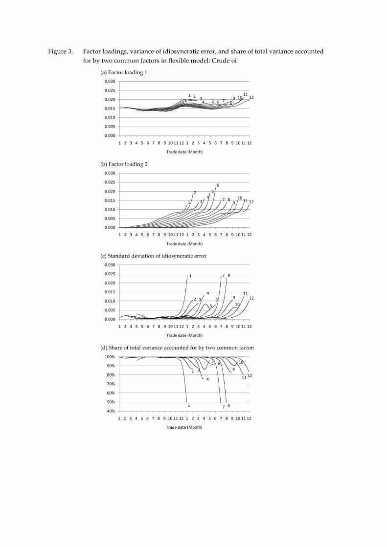
Figure 3.
(a) Factor loading 1
(b) Factor loading 2
(c) Standard deviation of idiosyncratic error
(d) Share of total variance accounted for by two common factors
Factor loadings, variance of idiosyncratic error, and share of total variance accounted
for by two common factors in flexible model: Crude oil
1 234 5 6 7
89 10
1112
0.000
0.005
0.010
0.015
0.020
0.025
0.030
121110987654321121110987654321
Trade date (Month)
1
2
34
5
6
7 89
1011 12
0.000
0.005
0.010
0.015
0.020
0.025
0.030
121110987654321121110987654321
Trade date (Month)
1
2 3
4
5
6
7 8
9
10
1112
0.000
0.005
0.010
0.015
0.020
0.025
0.030
121110987654321121110987654321
Trade date (Month)
1
2 3
4
5
7
6
8
9
10
11 12
40%
50%
60%
70%
80%
90%
100%
121110987654321121110987654321
Trade date (Month)

Figure 4.
(a) Factor loading 1
(b) Factor loading 2
(c) Standard deviation of idiosyncratic error
(d) Share of total variance accounted for by two common factors
Factor loadings, variance of idiosyncratic error, and share of total variance accounted
for by two common factors in flexible model: Gold
24 6
810
12
0.0000
0.0005
0.0010
0.0015
0.0020
12111098765432112111098765432
Trade date (Month)
2
4 610
128
0.0100
0.0102
0.0104
0.0106
0.0108
0.0110
12111098765432112111098765432
Trade date (Month)
24
6 8
10
12
0.0000
0.0005
0.0010
0.0015
0.0020
12111098765432112111098765432
Trade date (Month)
24
6 8
10
12
98.0%
98.5%
99.0%
99.5%
100.0%
12111098765432112111098765432
Trade date (Month)

Figure 5.
(a) Variance attributable to two common factors
(b) Variance attributable to idiosyncratic error
(c) Share of varaince accounted for by two common factors
Factor loadings, variance of idiosyncratic error, and share of total variance accounted
for by two common factors in conventional two‐factor model: Natural gas
1 2
3
4 56
7 89 1011
1295%
100%
1 2 3 4 5 6 7 8 9 10 11 12
0.0000
0.0002
0.0004
0.0006
0.0008
0.0010
0.0012
121110987654321121110987654321
12
3
4
5 67
89
10
11
12
0.00000
0.00002
0.00004
0.00006
0.00008
121110987654321121110987654321
1 2
3
4 56
7 89 1011
12
75%
80%
85%
90%
95%
100%
121110987654321121110987654321
1 2 3 4 5 6 7 8 9 10 11 12
0.0000
0.0002
0.0004
0.0006
0.0008
0.0010
0.0012
121110987654321121110987654321
12
3
4
5 67
89
10
11
12
0.00000
0.00002
0.00004
0.00006
0.00008
121110987654321121110987654321

Figure 6.
(a) Variance attributable to two common factors
(b) Variance attributable to idiosyncratic error
(c) Share of varaince accounted for by two common factors
Factor loadings, variance of idiosyncratic error, and share of total variance accounted
for by two common factors in conventional two‐factor model: Corn
3 5 79 12
0.0000
0.0001
0.0002
0.0003
0.0004
0.0005
76543211211109876543211211109876543
3
5
7
9 12
0.00000
0.00001
0.00002
0.00003
0.00004
0.00005
76543211211109876543211211109876543
35
7
9 12
94%
96%
98%
100%
3 5 79 12
0.0000
0.0001
0.0002
0.0003
0.0004
0.0005
76543211211109876543211211109876543
3
5
7
9 12
0.00000
0.00001
0.00002
0.00003
0.00004
0.00005
76543211211109876543211211109876543
35
7
9 12
80%
82%
84%
86%
88%
90%
92%
94%
96%
98%
100%
76543211211109876543211211109876543

Figure 7.
(a) Variance attributable to two common factors
(b) Variance attributable to idiosyncratic error
(c) Share of varaince accounted for by two common factors
Factor loadings, variance of idiosyncratic error, and share of total variance accounted
for by two common factors in conventional two‐factor model: Crude oil
1 2 3 4 5 6 7 8 9 10 1112
0.0000
0.0001
0.0002
0.0003
0.0004
0.0005
121110987654321121110987654321
1 2 3 4 567
8
91011 12
0.00000
0.00001
0.00002
0.00003
0.00004
0.00005
121110987654321121110987654321
1
2 34 5
6 7 8910
11 1299%
100%
1 2 3 4 5 6 7 8 9 10 1112
0.0000
0.0001
0.0002
0.0003
0.0004
0.0005
121110987654321121110987654321
1 2 3 4 567
8
91011 12
0.00000
0.00001
0.00002
0.00003
0.00004
0.00005
121110987654321121110987654321
1
2 34 5
6 7 8910
11 12
95%
96%
97%
98%
99%
100%
121110987654321121110987654321

Figure 8.
(a) Variance attributable to two common factors
(b) Variance attributable to idiosyncratic error
(c) Share of varaince accounted for by two common factors
Factor loadings, variance of idiosyncratic error, and share of total variance accounted
for by two common factors in conventional two‐factor model: Gold
24 6
8
10
1299.9%
100.0%
2 4 6 8 10 12
0.000100
0.000105
0.000110
0.000115
0.000120
1121110987654321121110987654321
2
4
6
8
10
12
0.0E+00
5.0E‐08
1.0E‐07
1.5E‐07
2.0E‐07
1121110987654321121110987654321
24 6
8
10
12
99.5%
99.6%
99.7%
99.8%
99.9%
100.0%
1121110987654321121110987654321
2 4 6 8 10 12
0.000100
0.000105
0.000110
0.000115
0.000120
1121110987654321121110987654321
2
4
6
8
10
12
0.0E+00
5.0E‐08
1.0E‐07
1.5E‐07
2.0E‐07
1121110987654321121110987654321

Figure 9.
(a) Variance attributable to two common factors
(b) Variance attributable to idiosyncratic error
(c) Share of varaince accounted for by two common factors
Factor loadings, variance of idiosyncratic error, and share of total variance accounted
for by two common factors in the composite model: Natural gas
5 7
90%
100%
1 2 3 4 5 6 7 8 9 10 11 12
0.0000
0.0002
0.0004
0.0006
0.0008
0.0010
0.0012
121110987654321121110987654321
1
2
3
4
5
6
7
8
9
10 11
12
0.0000
0.0002
0.0004
0.0006
0.0008
0.0010
0.0012
121110987654321121110987654321
1 2
3
4
5
6
7
8
9
10
11
12
40%
50%
60%
70%
80%
90%
100%
121110987654321121110987654321
1 2 3 4 5 6 7 8 9 10 11 12
0.0000
0.0002
0.0004
0.0006
0.0008
0.0010
0.0012
121110987654321121110987654321
1
2
3
4
5
6
7
8
9
10 11
12
0.0000
0.0002
0.0004
0.0006
0.0008
0.0010
0.0012
121110987654321121110987654321

Figure 10.
(a) Variance attributable to two common factors
(b) Variance attributable to idiosyncratic error
(c) Share of varaince accounted for by two common factors
Factor loadings, variance of idiosyncratic error, and share of total variance accounted
for by two common factors in the composite model: Corn
3 5 79 12
0.0000
0.0001
0.0002
0.0003
0.0004
0.0005
76543211211109876543211211109876543
3
5
7
9 12
0.0000
0.0001
0.0002
0.0003
0.0004
0.0005
76543211211109876543211211109876543
312
85%
90%
95%
100%
3 5 79 12
0.0000
0.0001
0.0002
0.0003
0.0004
0.0005
76543211211109876543211211109876543
3
5
7
9 12
0.0000
0.0001
0.0002
0.0003
0.0004
0.0005
76543211211109876543211211109876543
3
5
7
9
12
50%
55%
60%
65%
70%
75%
80%
85%
90%
95%
100%
76543211211109876543211211109876543

Figure 11.
(a) Variance attributable to two common factors
(b) Variance attributable to idiosyncratic error
(c) Share of varaince accounted for by two common factors
Factor loadings, variance of idiosyncratic error, and share of total variance accounted
for by two common factors in the composite model: Crude oil
1 2 3 4 5 6 7 8 9 10 11 12
0.0000
0.0002
0.0004
0.0006
0.0008
0.0010
121110987654321121110987654321
1
23
45 6
7
8
9
10
11
12
0.0000
0.0002
0.0004
0.0006
0.0008
0.0010
121110987654321121110987654321
3
5
6
10
80%
90%
100%
1 2 3 4 5 6 7 8 9 10 11 12
0.0000
0.0002
0.0004
0.0006
0.0008
0.0010
121110987654321121110987654321
1
23
45 6
7
8
9
10
11
12
0.0000
0.0002
0.0004
0.0006
0.0008
0.0010
121110987654321121110987654321
1
2
3
4
5
6
7 8
9
10
11
12
30%
40%
50%
60%
70%
80%
90%
100%
121110987654321121110987654321

Figure 12.
(a) Variance attributable to two common factors
(b) Variance attributable to idiosyncratic error
(c) Share of varaince accounted for by two common factors
Factor loadings, variance of idiosyncratic error, and share of total variance accounted
for by two common factors in the composite model: Gold
2 4 6 8 10 12
0.000110
0.000115
0.000120
0.000125
0.000130
1121110987654321121110987654321
24
6 8
10
12
0.0E+00
5.0E‐07
1.0E‐06
1.5E‐06
2.0E‐06
1121110987654321121110987654321
2
4
6 8
1299.5%
100.0%
2 4 6 8 10 12
0.000110
0.000115
0.000120
0.000125
0.000130
1121110987654321121110987654321
24
6 8
10
12
0.0E+00
5.0E‐07
1.0E‐06
1.5E‐06
2.0E‐06
1121110987654321121110987654321
2
4
6 8
10
12
98.0%
98.5%
99.0%
99.5%
100.0%
1121110987654321121110987654321

Figure 13.
(a) Crude oil
(b) Natural gas
(c) Gold
(d) Corn
Position of contract included into the variance minimizing portfolio realtive to
the spot (nearby futures) position
0
1
2
3
4
5
1 2 3 4 5 6 7 8 9 10 11 12
Time of entry (Month)
Conventional 2‐factor Flexible composite
0
1
2
3
4
5
1 2 3 4 5 6 7 8 9 10 11 12
Time of entry (Month)
Conventional 2‐factor Flexible composite
0
1
2
3
4
5
1 2 3 4 5 6 7 8 9 10 11 12
Time of entry (Month)
Conventional 2‐factor Flexible composite
0
1
2
3
4
5
1 2 3 4 5 6 7 8 9 10 11 12
Time of entry (Month)
Conventional 2‐factor Flexible composite

Figure 14.
(a) Crude oil
(b) Natural gas
(c) Gold
(d) Corn
Optimal hedge ratio
0.9
1.0
1.1
1.2
1.3
1.4
1 2 3 4 5 6 7 8 9 10 11 12
Time of entry (Month)
Conventional 2‐factor Flexible composite
0.8
1.0
1.2
1.4
1.6
1.8
1 2 3 4 5 6 7 8 9 10 11 12
Time of entry (Month)
Conventional 2‐factor Flexible composite
0.98
0.99
1.00
1.01
1.02
1 2 3 4 5 6 7 8 9 10 11 12
Time of entry (Month)
Conventional 2‐factor Flexible composite
0.90
0.95
1.00
1.05
1.10
1.15
1.20
1 2 3 4 5 6 7 8 9 10 11 12
Time of entry (Month)
Conventional 2‐factor Flexible composite
Recommended