N94- 29671
TDA Progress Report 42-116 February 15, 1994
A Complex Symbol Signal-to-Noise RatioEstimator and ItS Performance
Y. Feria
Communications Systems Research Section
This article presents an algorithm for estimating the signal-to-noise ratio (SNR)
of signals that contain data on a downconverted suppressed carrier or the firstharmonic of a square-wave subcarrier. This algorithm can be used to determine the
performance of the full-spectrum combiner for the Galileo S-band (2.2- to 2.3-Gttz)
mission by measuring the input and output symbol SNR. A performance analysis
of the algorithm shows that the estimator can estimate the complex symbol SNR
using 10,000 symbols at a true symbol SNR of-5 dB with a mean of-4.9985 dBand a standard deviation of 0.2454 dB, and these analytical results are checked
by simulations of 100 runs with a mean of -5.06 dB and a standard deviation of0.2506 dB.
I. Introduction
Current plans are for the performance of the full-
spectrum recorder (FSR) and full-spectrum combiner
(FSC) for the Galileo S-band (2.2- to 2.3-Gttz) mission tobe measured by running symbol-error-rate (SER) curves
on the demodulated data. To do so, one needs to generate
test signals at various points of the system, and the test
signals must be consistent from one point to the other,
which may be difficult. The measurement can only bedone at the output of the demodulator, which means that
if the demodulator is malfunctioning, other modules (e.g.,
the FSR or FSC) cannot be tested. Also, since test signalsare needed, online testing is impossible.
To overcome the disadvantages of measuring the per-
formance from the SER curves, one would like to directly
measure the symbol signal-to-noise ratio (SNR) at various
points of the system. This means that the symbol SNR hasto be estimated through complex symbols. By complex
symbols, we mean the real symbols at an offset frequency
with in-phase (I) and quadrature (Q) components. This
article presents a complex symbol SNR estimator that es-
timates the symbol SNR of data with I and Q components
of a carrier and/or the first harmonic of a square-wavesubcarrier. This SNR estimator can be used to measure
the performance of the FSC as well as that of the complex
symbol combiner for the Galileo S-band mission.
The technique of the complex symbol SNR estimator is
similar to that of the split-symbol moments estimator [1,2],
except with complex symbols rather than real ones. Theidea behind splitting a real symbol into two halves and
correlating them (originally suggested by Larry Howard
[2]), is to get the signal power by correlating two halvesof a symbol, where the signal parts of the two halves of
232
https://ntrs.nasa.gov/search.jsp?R=19940025168 2019-05-18T06:34:41+00:00Z

the same symbol are correlated but the noises on the twohalves of the symbol are uncorrelated.
The same idea is applied here to the complex symbols,
with the assumption that the offset frequency is known.
The idea is to correlate the first half of a symbol with the
complex conjugate of the second half of the same symbol,
and then to take the real part to get the signal power multi-
plied by a factor that is a function of the offset frequency.
This factor can be divided out if the offset frequency is
known. The same step is repeated for N symbols, and the
results are averaged to get a better estimate of the signal
power.
The signal power plus the noise power can be obtained
by averaging the magnitudes squared of the sums of the
samples in a complex symbol over N symbols. The esti-
mate of the SNR ratio is then readily obtained. In the
next section, a brief description of the complex symbol
SNR estimator is given.
Some practical problems are not considered here. For
instance, the frequency offset may not be known and may
not be a constant. Also, if the symbol synchronization
is off, say by a sample, the performance of the estimator
will be affected, and in the future, the effect needs to be
quantified.
m 2
SNR = 2cr---_ (3)
Presented here is an algorithm to estimate this symbol
SNR. First, add all samples in the first half of a symbol
for I and Q separately,
N, 12-1
Y_dk = E Yl, k (4)I=0
Ns/2-1
/=0
Repeat the first step for the second half of the symbol
Ns - 1
= (61l=Ns]2
N8 - 1
= yq, (7)I=N$/2
II. Brief Description of the Estimator
For given samples of I and Q components of baseband
data with an offset frequency Wo, we wish to estimate the
symbol SNR. The I and Q components of the/th sample
in the kth symbol are expressed as follows:
m dYJ,k = _ k cos (CooIr_ + ¢o) + nz,_ (1)
m dYQ,k = -_ k sin (woIT, + ¢o) + nQ,_ (2)
where
I = O,...,N,-1k = 1,...,N
Here N, is the number of samples per symbol and is as-
sumed to be an even integer, T_ is the sample period, and
dk = +1 is the kth symbol. The noise samples in the Iand Q channels are assumed to be independent with zero
mean and equal variance _r_/N_. The true symbol SNR is
Multiply the I component of the first half of a symbol by
that of the second half; do the same for the Q components;
and add the results. This is.equivalent to taking the real
part of the product of the first half and the complex con-
jugate of the second half of a symbol. Repeat the same
procedure for N symbols, and average the results to obtain
the parameter rnp
N1
k----1
N
Nit----1
where
Y_k = Y_,rk + JY,_Q_ (9)
YPk = YZxk + JY_Q, (10)
233

Take the magnitude squared of the complex sum of the
two symbol halves, repeat for N symbols, and average theresults to obtain rnss
i N
rrt,_ : _ _ IY_k -4-Y_k 12 (11)k=l
Mathematical expressions for the complex symbol halves
Y_ and Yp_ and the parameters mp and m_ are given inAppendix A in terms of the underlying model parameters
of Eqs. (1) and (2). Finally, use mp and rn_ to obtain theestimated symbol SNR
1
E {SNR*} -_ g (_p,_,,) +
[" 2 82g X
OmpOm_s + m, Om_, )
(14)
where cr_ and cr2 are the variances of mp and m,smp ross
respectively, and coy (mv,m,,) is their covariance. The
variance of the estimate, SNR*, can be approximated by
[3, p. 212]
SNR* =
4rnp sinJ (woT,/2) /[sinc 2 (woT, u/4) cos (woT, u/2)]
rnss - mp (2 + 2/cos (woT_y/2))
(12)
where wo is the offset angular frequency, and T_y is thesymbol duration,
T,_ = N.Ts
The estimate, SNR*, defined in Eq. (12) is shown in
the next section to have an expected value equal to the
true symbol SNR defined in Eq. (3), plus some bias that
decreases with the number of symbols averaged. The vari-ance of SNR* is also derived in the next section as a func-
tion of the number of symbols averaged and the true sym-bol SNR.
III. Mean and Variance of Symbol SNREstimates
In Eq. (12), the estimate of the complex symbol SNR,
SNR*, is a function of the random variables rnp and mss.Let g denote that function
SNR* = g(mp, m.) (13)
Assume that g(mp, m,) is "smooth" in the vicinity of the
point (_p,_,_), where _p and m_s are the means of rnvand m,,, respectively. The expectation of the estimate,
SNR*, can then be approximated by [3, p. 212]
( o, )'. ( o, )'.
+ 20g Og0--_-p 0m,. cov (mp,m,,) (15)
In Eqs. (14) and (15), all the partial derivatives and the
covariance are evaluated at (_p,-_,,). Expressions for the
mean and variance of rnp, the mean and variance of m,,,
the covariance of mp and m,_, and the partial derivativesare derived in Appendices B through E, respectively. Sub-
stituting all the terms frorn the appendices into Eqs. (14)
and (15), the mean and variance of SNR* are obtained,
E {SNR*} = SNR+Ncos 2 (z/2)
)x + SNR - _ cos (z)
]+ SNR 2 (1- cos (z)) (16)
and
_ i [2 +SNR_______+SNR 2Ucos (z/2)
3 (z)) SNR3-_ (1-cos (z))]
(17)
234
where
and
C1
z = ¢ooTsy
sine (WoT, y/4)
sinc (woT,12)
IV. Analysis Verification
Two methods are used to verify the analytical resultsof the mean and the variance in the complex symbol SNR
estimation:
(1) Compare the numerical results of the analysis to sim-ulation results.
(2) Set the offset frequency to zero and compare the
performance of the complex symbol SNR estimatorand that of the real symbol SNR estimator.
A. Simulation Results
Simulation results for the mean and variance of SNR*
are shown in Figs. (1) and (2), and are compared to thetheoretical results of Eqs. (16) and (17). The analytical
and simulation results are also compared in Table 1. In all
cases, the offset frequency, fo = Wo/(27r), is set at 20 Hz.
The simulation results are based on 100 runs each, and the
simulated means and variances are obtained by averagingover the 100 runs.
B. Special Case
A special case is when the offset frequency wo = 0. Inthis case, the performance of the complex symbol SNR
estimator should reduce to that of the real symbol SNR
estimator given in [1] and [5], with N samples of pure noise
and N samples of the signal plus noise.
For this special case, the mean and variance of the com-
plex symbol SNR estimates reduce to
1
E{SNR*} = SNR+ _(1 +SNR) (18)
2 N(2 + 4SNR + SNI% 2)CrSNR. (19)
The analysis in [1], which assumed a constant signal level
for all the samples, is easily extended to cover the ease of a
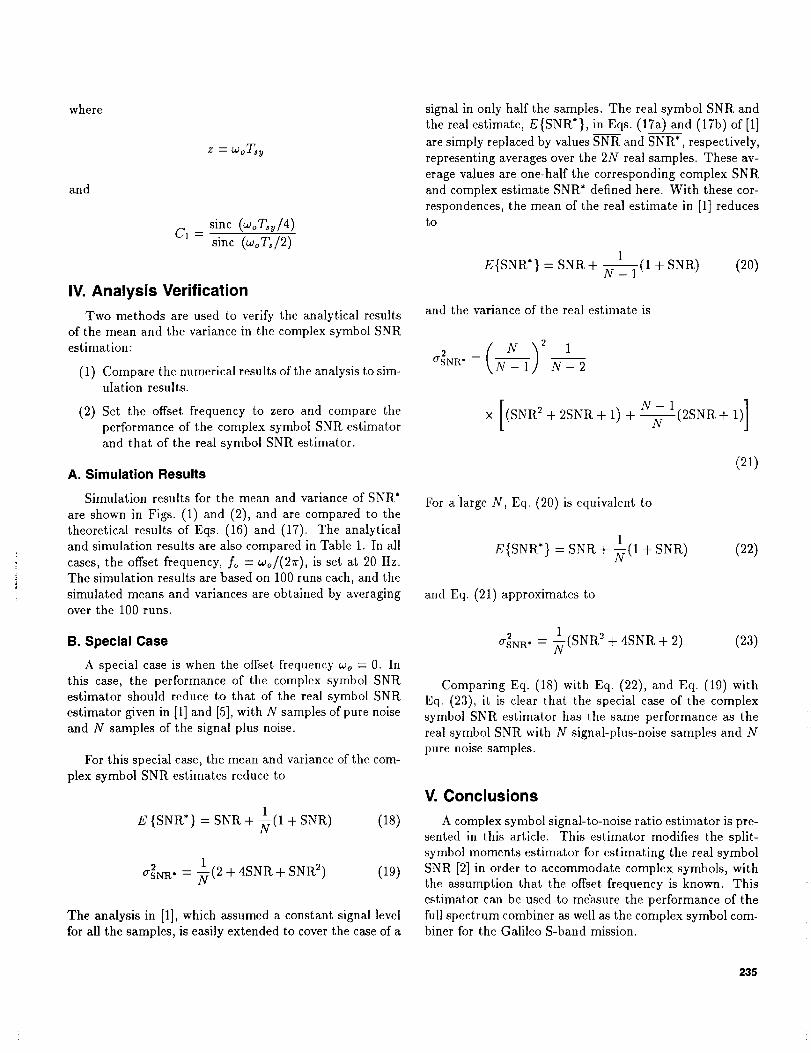
signal in only half the samples. The real symbol SNR and
the real estimate, E{SNR*}, in Eqs. (17a) and (17b) of [1]
are simply replaced by values SNR and SNR*, respectively,
representing averages over the 2N real samples. These av-
erage values are one-half the corresponding complex SNR
and complex estimate SNR* defined here. With these cor-
respondences, the mean of the real estimate in [1] reducesto
1E{SNR*} = SNR + _-Z-_(1 + SNR) (20)
and the variance of the real estimate is
(N__) 2 1gr2NR" = N- 2
x [(SNR2+2SNR+I)+-_--_(2SNR+I)]
(21)
For a large N, Eq. (20) is equivalent to
E{SNR*} = SNR+ 1(1 + SNR) (22)
and Eq. (21) approximates to
1 2
¢_NR" = _(SNR + 4SNR + 2) (23)
Comparing Eq. (18) with Eq. (22), and Eq. (19) with
Eq. (23), it is clear that the special case of the complex
symbol SNR estimator has the same performance as the
real symbol SNR with N signal-plus-noise samples and Npure noise samples.
V. Conclusions
A complex symbol signal-to-noise ratio estimator is pre-
sented in this article. This estimator modifies the split-
symbol moments estimator for estimating the real symbolSNR [2] in order to accommodate complex symbols, with
the assumption that the offset frequency is known. This
estimator can be used to measure the performance of the
full spectrum combiner as well as the complex symbol com-biner for the Galileo S-band mission.
235

Acknowledgments
The author would like to thank Sam Dolinar for his valuable contributions to this
work and Steve Townes for his many valuable suggestions and helpful discussions.
Special thanks are also due to Tim Pham for his great support of this work. The
author is grateful to Jay Rabkin for drawing her attention to this problem.
236

Table 1. Simulation results of the complex symbol SNR estimation.
Mean of SNR*, dB a of SNR*, dB
SNR, dB N Ns Runs
Theory Simulation Theory Simulation
-2 -1.9968 -2.0039 0.2956 0.2834 2,500 10 100
-2 - 1.9984 -2.0136 0.2112 0.1937 5,000 10 100
-5 -4.9985 -5.0589 0.2454 0.2506 10,000 10 100
-8 - 7.9986 -8.0437 0.3056 0.2787 20,000 10 100
237

m-o
¢-Zo9,_1o
OuJI--
I-.-
uJ
Z
LU
-1
-2-
-3 -
-4-
-5
-6
-7
--8
-9-9
I I i I I I (
N = ,5000
SIMULATED MEAN .,_
+1 STANDARD DEVIATION
THEORY
.r._._/ff_ N = 10,000
t"N=2o0oo
1 ! t I I I I
-8 -7 -6 -5 -4 -3 -2
ACTUAL SYMBOL SNR, dB
Fig. 1. Means and standard deviations of the symbol SNR estimates.
m 1.4"O
LMP- 1.2
_ 1.0uJ
Zco 0.8Z
z
o_ 0.6p-_<>
_ 0.4ai12
_ 0.2Z
_ 0.0
I I I t I I t
THEORY
• SIMULATION
- SNR = -8 dB
SNR = -5 dB
-2 dB
I I I I I I I
1 2 3 4 5 6 7
NUMBER OF SYMBOLS BEING AVERAGED, N x 104
Fig. 2. Standard deviations of the complex symbol SNR estimates.
238
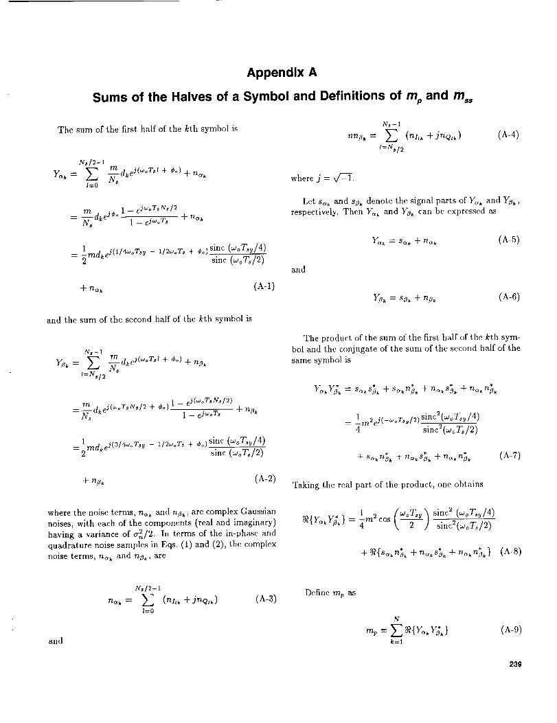
Appendix A
Sums of the Halves of a Symbol and Definitions of nip and mss
The sum of the first half of the kth symbol is
N./2-1
IVsl=0
rn .¢o ] -- e jw°TsNs/2= --dke; + n_k
Ns 1 - c jw°Ts
lmdkeJ(1/4woTsy - 1/2_oTs + ¢o)Sinc (woTsy/4)-- 2 sine (woT,/2)
+ nak (A-l)
Ns - 1
nnp. = E (nl, k + jnq,k) (A-4)
l=Ns/2
where j = v/L-] -.
Let s_ k and sp_ denote the signal parts of Y_ and Yp,,
respectively. Then Y_ and Y_k can be expressed as
YaK = s_k + n_,_ (A-5)
and
)_k = sz_ + nzk (A-6)
and the sum of the second half of the kth symbol is
Y_k
Ns -- l
l=Ns/2
__sdkeJ(woTsl + ¢o) -{-nBk
= rn dkcj(woTsNs/2 + ¢o) 1 -- ej(w°TsNs[2)N. 1 -- Cjw°Ts
-}- nflk
=l_mdkeJ(3/4w Tsy - l/2woTs + ¢o) sine (WoT_y/4)2 sinc (woT./2)
The product of the sum of the first half of the kth sym-
bol and the conjugate of the sum of the second half of the
same symbol is
_Ol k ")er_ k _ S* * $• Sak flk q- Sak n;k + nak SOL -}- nc_k nflk
_ 1 m2eJ(_woTs./2) sinc2(woTsy/4)4 sine_(woT_/2)
* * n* (A-7)+ sc_knfl_ + naksflk + n_k _k
-Jr ntis, (A-2) Taking the real part of the product, one obtains
where the noise terms, n_ and nzk , are complex Gaussian
noises, with each of the components (real and imaginary)
having a variance of _r_/2. In terms of the in-phase andquadrature noise samples in Eqs. (1) and (2), the complex
noise terms, na k and npk, are
_{y..y_}= l-m2cos(_-) sinc2(w°T'y/4)4 sinc=(_oT_/2)
* 8* rt* (A-8)
and
Ns/2-1
neck= E (nhk + JnQ'k) (A-3)I=0
Define mp as
N
k=l
(A-9)
239

The sum of the whole kth symbol is n.k = n& + jnQk (A-12)
Y_
Ns -- 1
mde j(w°TsI + ¢°) + nk}2m_/=0
_ rn dkeJ_o 1 - e jw°TsNs- N, I - e jw°Ts + nk
= rndkeJ(ll2_oT_u - ll2_oTs + _o) sine (woT_u/2) + nksine (woT_/2)
= sk + nk (A-10)
where sk is the signal part of tile whole symbol and nk is2 in eacha complex Gaussian noise with a variance of a,_
component (real and imaginary), and
8t: = sc_k + 8ilk
nk ---- nak -]- nflk
where Slk, sQk and nlk, nQk denote the I and Q com-ponents of the signal and the noise in the kth symbol.
Furthermore, }_, can be expressed as
}"_.= sIk + jsQk + nix + jnQk (A-13)
The sum squared of the kth symbol is
[y_12= _ sine2 (woT,,v/2),n _in----_ (_oT./2) + In_l=+ 2_{n_s;}
-- ,,,_c_+ In,.l"+ 2_{,,,..q.} (A-14)
where
sinc 2 (_oT,,y/2)
C_ = sinc"(_'oT,/2)
Note that the signal and noise parts of a whole complex
symbol, sx, and nk, can also be expressed in terms of their
in-phase and quadrature components, that is,
sl_ = Slk + jsQk (A-I1)
Define /ns._ as
N
,,.. = _ l)k.I_ (A-15)k=l
240

Appendix B
Evaluation of the Mean and Variance of mp
All the expectations in the following are conditional on
knowing the symbol synchronization.
N
1 _ E{Uk}E{mp} =k=l
I m2 sine 2 (woT, u/4)
N1 ,
+ _ _ z{_{s_k % + -°ks_ + ..k."k:l
Because the {Uk} are independent, the variance of mp
can be computed as [4, p. 352]
N
_2 1
k=l
Now let subscripts I and Q denote the in-phase and
quadrature components of the signals. The second mo-
ment of Uk can be expressed as
2
E{U:} = _" _ Ss2 82 s2
1 rn 2sine 2 (woT_u/4) (B-l)
where
= _{(=_ + "_)(=k + _5_)}
and s_ and sz_ denote the signal part of Y_ and YZk,respectively, as in Eqs. (A-5) and (A-6). The last step
in Eq. (B-I) follows from the independence of the noiseswith zero mean in the two halves of each symbol. Note
that T=y : N_T_.
4tT n
+ -_ + E{(f_ik=p_ + s.ekspe_) 2}
2 4
m 2 sinc2(woT_u/4) tr, + cf.___,2 sinc2(woT_/2) 2 2
+ E{(s.,ksp,k + S_qkSzqk) 2} (B-3)
Combining Eqs. (B-l), (B-3), and (B-2) yields
a2 1 {lm2sinc2 (woT, u/4) a2 _)m, = _ \4 sine 2 (woT,/2) '_ +(B-4)
241

Appendix C
Evaluation of the Mean and Variance of m,,
The mean of m., is
E{m,.} = E IYkt2 where
k=l
1 N 1 N
: m'C_+ _ _ EI._T_+ _ _ E{_{_4}}k=l k:l
= m2c_+ 2_ (C-l)
To find the variance of m., let
Yk = IYkl2
= Y,l+Y&
= (_.+ .,_)_+ (_Q_+ _q.)_ (c-2)
_ : E{t__}- (E{_,;])_ (C-4)
E_{v}: E'{m,.}
: (m_c_+ 2_}_)_ (o5)
Expanding V_, take the expectation of V_; apply
2 E{n_} E{n_} O, andE{_} = Z{_} : _, = =E{._ } = E{.$_} = 3_._ [3,p. 147];and usethe indepen-denceof n, k and nqk , and one will obtain
QO -2 {82E{v}} = 8_ + o _ ,, + _) + (d_ + _)_
x 8< + 8,n_c_o-_+ ,.._c_ (c-6)
The variance of Vk becomes
where Ylk, Yok, six, SQk, nlk, and nQk are defined in Ap-pendix A. Because the {Vk} are independent, the variance
of m. can be expressed in terms of the variance of Vk [4,
p. 352],
N
k=l
o-g,= ,,,n_Cfo-_+4o-,I (c-7)
Finally, the variance of m_ can be written as
_ = 1 [4,.2c_ + 4_] (c-8)m35 N
242

Appendix D
Evaluation of the Covariance of mp and m,,
The covariance of m v and ms_ is defined as
cog (m_, m..) : E{(,._ - _v)(m,. - _.)}
= E{mvm,, } - myra,, (D-l)
As in Appendices B and C, let
= Y_IkY_I_ + Y_QkY_Qk
= (_,_ + ,,.,_ )(_,_ + ,_,_)
+ (_,_ +._,_)(_,_ +._,_) (D-2)
and
V_
(D-3)
The expectation of the product of UkVk can be expressedas
E{ Uk Vk } =
O"n J- S,6zk 8ceQk 813Qk
_ .+ _-.,_c,_cos__. )
+ (r.(m C_) + (D-4)
where
sinc (woT_,/4)C1 =
sinc (woT,/2)
sine @oT,_/2)62 =
sinc (woT,/2)
and
Z = cgoT._y
Note that
C_ = 1612 [1 + cos (_)]
Then
E{mpmss } =
: k_ l:l
1E{UkVk} + E Z{Uk] E{Vz}N 2
k:l l:l,l;_k
1
N2 [NE{UkVk} + N_v(N - 1)_,,1 (D-5)
Finally, the covariance of m v and m,_ is
coy (.-,,,,m.) = _[E{U,_V,,} - .,,,m..]
: -- 2 2 21 [m C2(r,_ + _4] (D-6)N
243

Appendix E
Evaluation of the Partial Derivatives
Denote the following parameters in a convenient form,
4sine 2 (woTs/2)
I<1 = sinJ (woT_u/4) cos (woT_y/2)
2K2 : +2
cos @oLu/2)
02g ] 2Kl K2_p 2KIK2
2 c°s_(z/4) [ ( 2) 4] (E-3)_ cos_(z/2) 2SNR 1 + cos +
and
sine (woT.u/4)C1 --
sinc @°%/2)
Z : oJoTsy
In terms of K1 and Ks, the estimate SNR* defined in
Eq. (12) is given by
SNR* = g(m v, ,n,,)
Og _v,_ss I'(l g'_p8_. =- (-_. - l;_mp)2
= - _-_#12SNR (E-4)
029 t 2K,_p0_L _.,_.= (_._-l;_v)3
1
-- 2a4n SNR (E-5)
K 1 mp
_as-- K2mp
(e-l)
Then g(Tfip,_ss) = SNR, and the partial derivatives ofthis estimator function are
KI K2mp KI
(m_ - K2mv ) _ + --m. - K2-_v
z 22]1 SNR (1 +cos_) + __a cos (z/2)
(E-2)
029
Oln, pOm,s _'T_,-6_ss :
2K, K2_p K1
(-i-_ss -- /_-'27"_'p) 3 ('_ss -- /\"2_p) 2
cos(=/u)<SNR ,+cos + (E-6)
where the second lines of Eqs. (g-2) through (g-6) are
obtained by substituting the expressions for rg v = E{mp}
and i-fiss = E{m,s} from Appendices B and C.
244

References
[1] S. Dolinar, "Exact Closed-Form Expressions for the Performance of the Split-Symbol Moments Estimator of Signal-to-Noise Ratio," The Telecommunications
and Data Acquisition Progress Report 2_2-100, vol. October-December 1989, Jet
Propulsion Laboratory, Pasadena, California, pp. 174-179, February 15, 1990.
[2] L. IIoward, "Signal and Noise Measurements in the NASA Deep Space Network,"20th URSI Conference, Washington, DC, August 10 19, 1981.
[3] A. Papoulis, Probability, Random Variables, and Stochastic Processes, New York:
McGraw Hill, 1965.
[4] R. Fante, SignalAnalysis and Estimation, New York: John Wiley and Sons, 1988.
[,5] M. Simon and A. Mileant, "SNR Estimation for the Baseband Assembly," TheTelecommunications and Data AcquisitioT_ Progress Report 42-85, vol. Januarll-
March 1986, Jet Propulsion Laboratory, Pasadena, California, pp. 118 126, May
15, 1986.
245
Recommended