Download pdf - A COMPARISON OF THREE MULTIVARIATE STATISTICAL TECHNIQUES ... P295-308_A... · studies in avian biology no. 13:295-308, 1990. a comparison of three multivariate statistical techniques

Studies in Avian Biology No. 13:295-308, 1990.

A COMPARISON OF THREE MULTIVARIATE STATISTICAL TECHNIQUES FOR THE ANALYSIS OF AVIAN FORAGING DATA

DONALD B. MILES

Abstract. This study discusses the complexities of analyzing foraging data and compares the performance of three multivariate statistical techniques, correspondence analysis (CA), principal component analysis (PCA), and factor analysis (FA) using five sample data sets that differ both in numbers of species and variables. Correspondence analysis consistently extracted more variation from the data sets (measured per eigenvalue or cumulatively) than either PCA or FA. Percent variance associated with the first axis and cumulative variance associated with the first five axes were negatively correlated with sample size, although the trend was stronger with PCA. There was also a significant positive relationship between percent variance and number of variables for PCA. CA showed a similar but nonsignificant trend. All three methods exhibited the “arch” effect or curvilinear&y of the data when the positions of species were plotted along the first two derived axes. This suggests that the curvature trend in foraging data may represent a characteristic of the data rather than be solely an artifact of data reduction. Consistency in the biological interpretation of the derived foraging axes was determined using an analysis of concordance. Of the three methods, PCA and CA showed a high level of consistency in magnitude and sign of the coefficients from the first three eigenvectors. The concordance of the results from a factor analysis with the other two methods was low. Further, jackknife and bootstrap analyses revealed relatively stable estimates of the eigenvectors for only CA and PCA. Overall the analysis indicates that CA is a preferred method for analyzing foraging data.

Key Words: Foraaina behavior; multivariate analysis; correspondence analysis; principal component analysis; factor a&y&; jackknife; bootstrap.

Many analyses of avian ecology, particularly community oriented studies, rely on data rep- resenting the foraging behavior of coexisting species to address questions pertaining to guild structure, resource partitioning, community organization, habitat use and competition (e.g., Holmes et al. 1979b, Landres and MacMahon 1983, Sabo 1980, Sabo and Holmes 1983, Miles and Ricklefs 1984, Morrison et al. 1987b). Be- cause most community studies assume that the manner in which a species exploits food re- sources represents an important niche dimension, a primary goal is to describe such resource axes indirectly through the measurement of foraging behavior. Thus, these studies attempt to estimate an unknown and underlying gradient of foraging behavior. Having determined this gradient, species may be positioned relative to one another along a foraging axis and inferences drawn about the ecological determinants of resource partitioning, guild structure, or community organization.

The resulting data set from a behavioral study of avian foraging usually consists of many variables measured on several species. Consequent- ly, the investigators may choose to extract the key relationships embedded in the multidimensional data through a multivariate analysis. Sev- eral methods have been used to derive resource (niche) axes or foraging gradients from foraging behavior data. One approach adopted by avian ecologists for analyzing foraging data has been

cluster analysis, based on various distance or similarity metrics (e.g., Landres and MacMahon 1980, Airola and Barrett 1985, Holmes and Recher 1986a). However, many investigators have turned to more advanced multivariate techniques, namely ordination methods, for deriving ecological patterns in multidimensional data. The prevalent ordination methods used in avian foraging studies include principal component analysis (Landres and MacMahon 1983, Leisler and Winkler 1985) factor analysis (Holmes et al. 1979b, Holmes and Recher 1986a) and correspondence analysis (Sabo 1980, Miles et al. 1987).

While several studies have compared the performance of multivariate methods in relation to vegetational gradients (e.g., Fasham 1977, Gauch et al. 1977) few attempts have used foraging data (Sabo 1980, Austin 1985). This paper assesses the “best” method for analyzing foraging data and tests the degree to which the unique characteristics of such data, in particular the “constant sum constraint,” affect the results from a principal component analysis and factor analysis. Data from five avian studies spanning four habitat types (Sub-Alpine Forest, Deciduous Forest, Desert Scrub and Evergreen Oak Wood- land) were analyzed using principal component analysis (PCA), factor analysis with Varimax rotation (FA), and correspondence analysis (CA). The criterion employed to determine efficacy of analysis was the percent variance summarized by the first four axes. Because many significance

295

296 STUDIES IN AVIAN BIOLOGY NO. 13

tests of multivariate methods require large sample sizes and most data infrequently meet this assumption, I generated standard errors and confidence limits for the coefficients and eigenvalues associated with each multivariate technique by jackknife and bootstrap procedures (Mosteller and Tukey 1977, Efron 1982).

CHARACTERISTICS OF FORAGING BEHAVIOR DATA

Investigations of avian foraging behaviors often depend on data gathered by observational methods. In such studies, a priori decisions are made about the types of foraging categories to recognize; these include the distinctiveness of various foraging substrates and the characterization of the foraging repertoire. Hence the range of categories included is determined by the ecological perceptions and subjective biological judgment of the investigator; the inclusion or definition of a category is largely arbitrary. Further, the non- independent nature of most foraging observations, which is affected by the particular design of the study, presents an additional complication in the analysis ofresource exploitation. The latter point may be addressed by using an appropriate sampling design when collecting the foraging observations. Accordingly, the choice of statistical technique for analyzing foraging data is con- strained by these inter-relationships among the variables.

The analysis of foraging data presents two major difficulties; one involves a biological dilem- ma, and the second is one of statistical assumptions. Data collected on the foraging behavior of species may be envisaged to consist of observations apportioned among various cells in a multidimensional contingency table (see Miles and Ricklefs 1984). Such a contingency table represents a classification of foraging techniques by the type of substrate. A frequent method of analyzing such data is to treat each category as a separate, independent variable and use PCA or FA on the correlation matrix. However, such a procedure ignores the underlying relationships and biological interdependencies among the foraging variables and arbitrarily adds dimensions to the ecological space. That is, certain combinations of maneuvers and substrates are more likely to be employed because of energetic or biomechanical factors. Yet, other combinations may be physically unavailable to a species. For example, techniques such as gleaning, hovering, and probing may represent intermediate points along an underlying continuum. Similarly, foraging substrates may be intuitively ordered in some unknown manner, such as from coarse substrates, trunk and branches, to finer substrates, such as leaves. Overall, we may imagine that

gleaning and hovering at leafy substrates lie at one end of an axis, and probing or pecking at ground substrates fall on the opposite end. Therefore, we may be justified in the assumption that the cross-tabulated foraging categories are discrete estimates of a continuous ecological axis that is to be estimated.

A second characteristic of foraging data is that the measurements are frequencies rather than continuous variables. This presents difficulties in the use of ordination techniques such as principal components analysis. Two main problems emerge by transforming the data from raw counts to proportions. First, frequency data exhibit marked curvature (Aitchison 1983). Second, as has been recognized in geological analyses, correlations among proportions may be subject to misinter- pretation. When a vector of raw counts for p observations (x,, . . , x,) is normalized, that is Y, = x,/p (Xl, . . 3 x,) it becomes a vector of proportions (or compositional data) that are correlated. This property of frequency data has been termed the “constant sum constraint” by Aitchi- son (198 1, 1983) because the terms in each vector must sum to unity. This constraint restricts the estimates of the correlation structure of the variables and results in a bias towards negative correlations. The statistical problem involves the recognition of this artifact, that is, how can the correlations that are artificially negative be de- tected. Thus, a principal component analysis of a categorical matrix may result in a biologically uninterpretable space. Such a conclusion leads to the question “how can foraging data be analyzed?’ Further, can we develop confidence limits for our estimates? A comparison of the analysis of frequency data using several multivariate techniques may yield important insights into their behavior and biases.

EVALUATION OF MULTIVARIATE TECHNIQUES USED IN FORAGING ANALYSES

A chief goal of most investigations of avian foraging behavior is to summarize a cross-tabulated matrix of maneuver by substrates in a few axes that accurately represent the interrelationships of the species. Thus, we wish to position species along a foraging continuum that may be used later for interpreting those factors respon- sible for separating species in the ecological space; that is, we may look for clumping or clustering of species, which would suggest possible guilds. Further, we may be interested in discovering those foraging variables that contributed most to determining the inferred guild structure. Because the multivariate methods are used both to reduce a complex multidimensional data set to a lower number of uncorrelated variates or axes, and to position species along these derived gradients,

MULTIVARIATE ANALYSES OF FORAGING--Miles 297

one must examine the assumptions and prop- erties of the three commonly employed multivariate techniques as well as the biological in- terpretability of these techniques.

Principal component analysis

The most prevalent technique used for analyzing foraging variables is principal component analysis (PCA). It is a variance-maximizing procedure, based on a Euclidean distance metric. PCA derives a small number of independent axes that extract the maximum amount of variance from the original data (Dillon and Goldstein 1984, Pielou 1984). No assumptions are necessary about the distribution of the data used by the method, although the data are assumed to be linearly or at least monotonically distributed. However, to perform significance tests of the eigenvalues one must assume that the data are approximately multivariate normally distributed. Apart from calculating the covariance or correlation matrix, PCA does not estimate param- eters that fit an underlying statistical model. PCA is not scale invariant; variables that differ in units of measurement or vary in magnitude will affect the results. Because PCA attempts to maximize the total variation in a reduced number of axes, those variables with the highest variance will tend to contribute more to the derived axes. Many studies avoid the problems of scale in PCA by standardizing the variables by their corresponding standard deviation. This procedure concom- itantly distorts the distances between points. Consequently the derived principal axes are unique to the particular data set and preclude generalizations from one study to another.

PCA transforms the original data matrix, com- posed of many presumably intercorrelated variables, into a reduced set of uncorrelated linear combinations that account for most of the variance present in the original variables. The first principal component (PC 1) is the linear combination that accounts for the greatest amount of variation relative to the total variation in the data. The second principal component (PC 2) extracts the largest amount of remaining variation, subject to the condition that it is uncorrelated (orthogonal) to the first. Similarly, PC 3 is calculated as the linear combination of original variables with the largest amount variance, but it is uncorrelated to the second and first PC axes.

Interpretation of the principal axes is arrived at by inspection of the coefficients of the eigenvectors and the correlations of the original variables with the principal component or component loadings. Because all principal components are linear combinations of the original data, the orientation of the axis projected through the cloud of points that maximizes the explained variation

is determined by the coefficients of each eigenvector. The contribution of a variable to the principal component axis is determined by an examination of sign and magnitude of the component loadings (Dillon and Goldstein 1984).

Factor analysis Whereas PCA is concerned with maximizing

the total variation in a reduced number of axes to arrive at a more parsimonious representation of the data, FA is a technique for determining the intercorrelation structure among the variables (Dillon and Goldstein 1984). That is, FA attempts to portray the interrelationships among the variables in a reduced number of axes that maximize the variance common to the original variables. Implicit in this definition of a FA model is the assumption that a variable may be par- titioned into two components, a unique factor and a common factor. As the terms suggest, the common factor represents an hypothetical and unobserved variable that jointly shares a fraction of the variation among all variables; the unique factor is an unobserved, hypothetical variable in which the variation is fixed and distinct to one variable. A second assumption made in FA is that the unique fractions are uncorrelated both with one another and with the common fraction. Thus, the factor analytic model is an analysis of the common variation among the variables (Dil- lon and Goldstein 1984). FA may be summarized by the model

X= Af + e,

where X is the matrix of observations, f is a matrix of the unknown and hypothetical common factors, e is a matrix of unique factors, and A is a matrix of unknown factor loadings. Simply stated, FA seeks to describe the complex relationships that characterize the observed variables in terms of a few, unknown, unobservable quantities known as factors. These factors allow one to determine the structure of the data and to derive common axes that unite the variables. However, few ecologists have critically examined the extent to which the factor model is rel- evant for their analytical goals. Because of the complex nature of the factor model and the assumptions made about the nature of the variation associated with the variables, ecologists must be keenly aware of the differences between FA from PCA before deciding on an analytical technique. Direct solution of the complex factor model is difficult, because of the presence of several hypothetical and unknown quantities (Dil- lon and Goldstein 1984). A common approxi- mate solution is given by a principal component analysis of the reduced correlation matrix (i.e., a correlation matrix that has had the unique vari-


ation removed). In this solution an estimate of the unknown matrix of factor loadings is derived by multiplying each element of the eigenvectors by the square root of the corresponding eigenvalue. The “meaning” of each factor axis, in terms of identifying the underlying pattern of variation that is common to the variables, usually proceeds by the examination of the magnitudes of all loadings. A variable is retained for interpretation if it exceeds a critical threshold, which may be defined either arbitrarily, as in a loading exceeding a certain minimum value, or by the statistical significance of the loading.

Orthogonal rotation of the factor axes often follows the extraction of the components as an aid to interpretation of the extracted factor pattern. The justification for rotating the axes is, in most instances, that the factor pattern may be difficult to interpret; one or two variables might have high loadings, but most may be of similar magnitude. This additional transformation of the factor axes is coupled with the goal of restricting the interpretation of each axis to as few of the variables as possible. The most commonly used method, Varimax rotation, seeks to maximize the square of the factor loadings. The end result is an exaggeration of the magnitude of the loadings: the larger loadings are made larger and the smaller loadings are diminished (Dillon and Goldstein 1984). Most examples of FA in the ecological literature simply employ a Varimax rotation of the derived PCA axes. Several dis- advantages accompany the use of FA. First, the solution to the factor model is unique to the particular study. That is, it is very difficult to gen- eralize the results of one study to another. Sec- ond, the rotation of the axes distorts the distance relationships among the observations, which precludes comparing the positions of species in the ecological space from one study to another.

Correspondence analysis

Correspondence analysis, also known as recip- rocal averaging analysis (Hill 1974, Miles and Ricklefs 1984, Moser et al., this volume) is a dual ordination procedure. Both species and foraging categories are analyzed simultaneously on separate but complementary axes. The disper- sion of species is accomplished by means of the distributions across foraging categories. Con- versely, the categories are ordinated according to the patterns of their use by each species. The technique reveals the presence of underlying ecological and phenotypic variables pertinent to the manner in which birds forage (Sabo 1980, Miles and Ricklefs 1984).

Correspondence analysis uses an eigenvector algorithm similar to that of PCA (Hill 1973, 1974; Gauch et al. 1977; Pielou 1984). However, it

differs from PCA in three principal qualities: (1) the use of chi-square distances rather than Eu- clidean; (2) a double standardization of the data; and (3) an additional division step (Gauch et al. 1977). This first quality is useful, for it allows confidence intervals to be placed about points in the reduced space. Axes are computed that maximize the correspondence between species and the foraging categories. As in PCA and FA, the number of CA axes required to explain most of the variation in the data set is fewer than the number of categories in the original matrix. One advantage of CA is its resistance to distortion when analyzing curvilinear or nonmonotonic data (Gauch et al. 1977, Lebart et al. 1984, Moser et al., this volume).

I specifically did not include detrended correspondence analysis in this study (Sabo 1980) because of its use of an arbitrary, ad hoc standardization of the second and successive axes based upon the assumption of a single dominant axis. It further employs a resealing of the data as an aid to interpret intersample distances (Miles and Ricklefs 1984, Pielou 1984). In a study comparing four ordination methods, Wartenberg et al. (1987) showed that detrended correspondence analysis and CA arrived at a similar ordering of species along a single gradient. For a detailed discussion of the weaknesses of detrended correspondence analysis see Wartenberg et al. (1987).

MATERIAL AND METHODS I analyzed five sets of data (Table 1) that had the

following dimensions: 20 species by 14 variables, 19 species by 14 variables, 11 species by 16 variables, 14 species by 15 variables, and 12 species by 15 variables. Because the data consisted of proportions, I used the arcsine-square root transformation before performing the PCA or FA.

Each data set was subjected to analysis by CA, PCA, and FA. The last two techniques had as input the correlation matrices generated from the foraging data. To make comparisons among studies I followed the methods of previous studies, and used the principal factor method to derive a reduced set of factor axes in the FA. All factor axes whose associated eigenvalues exceeded one were used in subsequent analyses. Next, I performed a Varimax orthogonal rotation of factor axes to further reduce the structure of the data to a few combinations of original variables. In this study, PCA and FA extracted eigenvalues using a similar algorithm and generally arrived at common solutions, therefore I only analyzed the PCA eigenvalues for patterns in explained variance. Unlike the previous two analyses, CA was performed using the untransformed proportions. Interpretation of the results was accomplished by a simultaneous plotting of the foraging category coordinates and the species (sample) coordinates. The magnitude and sign of the coordinate indicates its contribution to the structure of the data. Previous evalu- ations of CA considered it to lack rigorous statistical tests for the eigenvalues and eigenvectors. However,


TABLE 1. SOURCES OF FORAGING DATA ON PASSERINE USED IN THIS STUDY

Number Number of of

LocatIon Habitat type species variables SClUKe

Mt. Moosilauke, New Hampshire Hubbard Brook, New Hampshire Purica, Mexico

Santa Rita Mtns., Arizona Saguaro National Monument, Arizona

Sub-alpine forest 20 14 Deciduous forest 19 14 Evergreen oak 11 16

woodland Encinal 14 15 Desert scrub 12 15

Sabo (1980) Holmes et al. (1979b) Landres and MacMahon

(1980) Miles (unpubl. data) Miles (unpubl. data)

the unique distributional qualities of chi-square distances allow for several significance tests (see Lebart et al. 1984).

dence limits about a complex statistic that lacks an analytical sampling distribution.

All three multivariate techniques share two common goals: (1) the determination of common themes of co- variation among a strongly correlated group of variables and (2) the reduction of a high-dimensional data set into a few derived axes that preserve as much of the original variation as possible. Therefore, I based my evaluation of the performance of these procedures on the percent variation extracted per axis. This criterion allows a direct comparison of PCA and CA whose eigenvalues are not interchangeable. I examined (1) the number of axes necessary to explain at least 90% of the variation and (2) the proportion of variation associated with the first axis. The multivariate technique that consistently explained a larger fraction of the original variation in the least number of axes and resulted in easily interpretable axes should be preferred. This also has direct bearing on the number of axes to retain for subsequent analyses and interpretation. Because most studies that use multivariate techniques depend on the loadings for interpreting the results, I compared the three procedures for consistency in the direction and magnitude of the axis loadings.

The premise ofthe jackknife is to determine the effect of each sample on a statistic by iteratively removing successive samples and recalculating the statistic (Mos- teller and Tukey 1977, Efron 1982, Efron and Gong 1983). The jackknife analysis begins by computing the desired statistic for all the data. A single observation is then removed from the data and the statistic is re- calculated using the remaining n - 1 observations. Let y,,, represent the statistic calculated for the full sample. Define a pseudovalue to equal

y* = ny,,, - (n - lly,,, j = 1, 2, , n, where n is the sample size. The jackknifed estimate of the statistic is defined as the mean of the pseudovalues

y* = l/n 2 y* I’

and the variance of the jackknifed statistic is given by

s** = r(y*, - y*)Vn(n - 1)]“,

where s2 is the variance of the pseudovalues. One can use the jackknife estimate of variance to calculate confidence intervals based on the t distribution (Mosteller and Tukey 1977).

Jackknife and bootstrap estimation of variability

Several common problems plague ecological investigations that employ multivariate methods. The first is how many axes should be interpreted, or kept for further analyses. The second involves which of the coefficients in the eigenvectors may be used to interpret the patterns suggested by a PCA or CA. Because of the small sample sizes, unknown sampling distribution, and the large number of categories that characterize foraging studies, formal statistical testing of eigenvalues is impossible. Consequently, predominant solutions to the above dilemmas are actually ad hoc guidelines. Computation of PCA by using the correlation matrix further complicates hypothesis testing, for most of the statistical tests are based on the variance-covariance matrix.

I used the jackknife method of variance estimation for the principal component analysis, factor analysis, and correspondence analysis of foraging data from all five data sets. Two statistics were subjected to this resampling plan. Upon deleting a single observation from the original data set and recalculating the three multivariate procedures, I derived the pseudovalues for the first four eigenvalues and the elements of the first three eigenvectors. This procedure resulted in the calculation of jackknife estimates of the statistics and a measure of their variability. Following Mosteller and Tukey (1977) I also computed the jackknife error ratio, which is simply the jackknife estimate divided by its standard error. The ratio may be viewed as a t statistic with (n - 1) degrees of freedom. Because the results of the jackknife method were similar for all data sets, in this paper, I present only the results for the Santa Rita data set.

However, bootstrap and jackknife resampling tech- The bootstrap is a conceptually simple, but com- niques can replace the arbitrary and ad hoc procedures. puter-intensive, nonparametric method for determin- Both are receiving increased use in ecological studies ing the statistical error and variability of a statistical (e.g., Gibson et al. 1984, Stauffer et al. 1985). Their estimate. The premise of the bootstrap is that, through use provides an estimate of a statistic as well as a resampling of the original data, confidence intervals measure of variance associated with the estimate. These may be constructed based on the repeated recalculation methods are particularly crucial for deriving confi- ofthe statistic under investigation. An assumption made


TABLE 2. PERCENT VARIANCE EXPLAINED BY THE FIRST FNE EIGENVALUE~ FROM PRINCIPAL COMPOIW~~ ANALYSIS AND CORRESPONDENCE ANALYSIS

Sample

Axis

I II III IV V

PCA CA PCA CA PCA CA PCA CA PCA CA

Mt. Moosilauke 27.3 36.7 23.4 20.1 16.2 18.4 9.2 9.7 6.6 6.2 Hubbard Brook 27.5 32.4 23.1 28.6 14.7 12.1 12.3 10.4 7.2 9.0 Purica 37.1 41.9 19.4 28.7 13.7 12.7 9.2 8.7 7.9 5.1 Santa Rita 31.6 33.5 21.4 30.0 15.8 13.9 11.3 10.7 6.4 4.5 Saguaro 39.4 36.1 19.7 31.1 12.4 12.2 8.2 8.2 6.3 5.2

by the bootstrap is that the data follow an unknown but independent and identical distribution.

To begin the bootstrap procedure, the following steps were executed. First, I pooled the original data set con- sisting of n observations. Using a random-number gen- erator, I selected n observations from the data with replacement; these n random values constituted a bootstrap sample, x*,. That is, each individual observation was independently and randomly drawn and subsequently replaced into the original data before another observation was drawn. A consequence of this sampling scheme was that an observation could be represented more than once or not at all in any bootstrap sample. The data were resampled a large number of times, which resulted in m bootstrap samples. Next, the statistic of interest was computed for each of the m bootstrap samples. In the present study, I calculated bootstrap estimates of the eigenvalnes and eigenvectors only from a PCA. Let L*; designate the ith bootstrap calculation of the jth eigenvalue or eigenvector. Then the bootstrap estimate of either statistic and the associated standard error is

L, = I/m z L*;

SE(-&‘) = a, where s2 = the variance of the m bootstrap L*; samples, i.e., (L*‘,, L*:, . . . , L*“,). The estimated mean and standard deviation of the PCA statistics were based on 200 bootstrap replications. This bootstrap sample size was the first from a range of sample sizes (100, 200, 300,400, and 500) to exhibit a stable convergence with the bootstrap calculations based on larger replicates.

In this study, the correspondence analysis, factor analysis, principal component analysis and bootstrap analysis were performed on an IBM 4381 using the following programs: CA, CORRAN (modified from Lebart et al. 1984) PCA and FA, SAS (SAS 1985). The program to compute the jackknifed statistics was written in QuickBASIC (version 3.0) and was performed using and IBM PC compatible computer.

RESULTS

Percent variance explained FA and PCA arrived at a similar set of eigen-

values, so results for only the latter analysis are provided. Percent variance explained by the first two axes was generally higher for CA than PCA

(Table 2) although PCA explained a higher amount of variation than CA in the first axis for the Saguaro data, and PCA had a higher percent variation value than CA in the second axis for the Mt. Moosilauke data. Along the third, fourth and fifth axes, PCA had higher values of percent variance extracted than CA for most data sets (Table 2). However, several of the comparisons were very similar (e.g., axis IV for the Saguaro data set and axis V for the Mt. Moosilauke data). The tendency for CA to capture more variation in the first few axes was biologically meaningful, for it suggests that CA may be more efficient at describing the underlying continuum that may characterize foraging behavior.

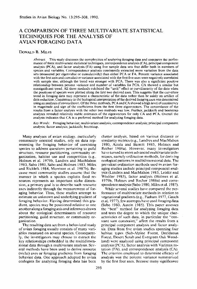
Cumulative variance for the first seven axes ranged from 97% to 99% for the CA results and 90% to 95% for the PCA (Fig. 1). CA would retain the first four or five axes to explain 90% of the variation (one criterion for determining the number of axes to retain and interpret), while PCA would require at least six axes and in one case seven axes. Thus, based on these results, CA pre- serves most of the original information in a reduced number of axes.

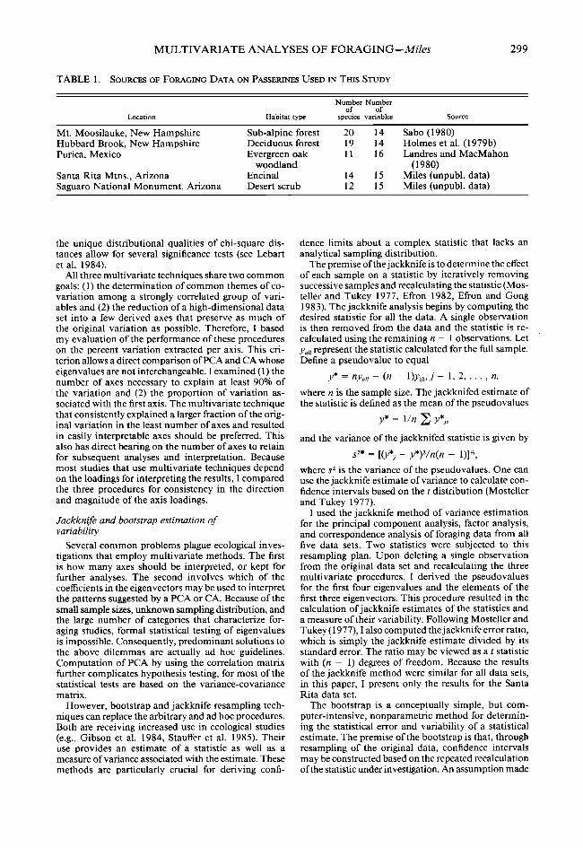
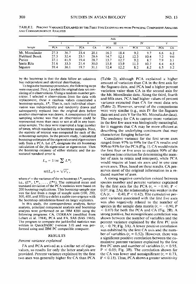
A strong negative correlation existed between species number and percent variance explained by the first axis for the PCA (v, = -0.90, P < 0.07; Fig. 2A); the relationship was weaker in the CA (rs = -0.40, P < 0.42). The cumulative percent variance associated with the first five axes was also negatively related to the number of species in the sample data matrix (rs = -0.90, P < 0.07) for both the PCA and CA (Fig. 2B). A strong positive, but nonsignificant correlation was shown between the number of variables and the percent variance explained by the first PC axis (T$ = 0.79; Fig. 3A). A lower positive correlation was exhibited by the first CA axis and the number of variables (rs = 0.52). However, there was a significant positive correlation between the cumulative percent variance explained by the first five PC axes and number of variables (T$ = 0.95, P < 0.05; Fig. 3B). The correlation shown for the CA was lower and nonsignificant (rs = 0.73, P < 0.15). Thus, PCA shows a greater sensitivity


to changes in the number of foraging variables included in an analysis than CA.

Presence of the arch effect

In this study, the distortion of the second and higher axes was present in all three multivariate methods (Figs. 4, 5, 6; see also Fig. 1 in Moser et al., this volume). The positions ofspecies along the first two axes from a CA, PCA and FA exhibited a characteristic v-shaped pattern or arch effect. The degree of distortion also was similar for all three analyses. One frequent criticism of CA is the tendency for the distribution of species to be compressed towards the terminal portions of the axes. However, the plot of CA axes 1 and 2 failed to demonstrate any compression of points along the axes.

Dzferences in interpretation of resource axes

The interpretations derived from one analysis of the foraging data were not necessarily sub- stantiated or similar when applying a second multivariate method. As an example, the second axis from a CA of the Santa Rita data (Table 3) described a gradient with gleaning at leaves and twigs at one end and gleaning and probing of trunks, branches, and ground at the other. How- ever, the interpretation from FA revealed that the axis described a contrast between hovering at leaves, twigs, and branches against gleaning maneuvers. Although not presented, dissimilar- ities in the biological interpretation among the three multivariate techniques were also evident in the other four data sets.

Greater than 73% (1 l/15) of the paired comparisons between CA and PCA were statistically significant based on Kendall’s rank order correlation coefficient (Table 4). Fewer than 50% of the correlations between CA and FA were significant (7/ 15). The degree of concordance between PCA and FA was also low; only 53% of the comparisons showing significant correlations.

Jackknife and bootstrap variance estimates CA and PCA exhibited similar results of jack-

knife and bootstrap analyses for all three axes (Tables 5 and 6). Because the results from all five data sets were the same, I present the jackknifed coefficients from only the Santa Rita data set. A coefficient was considered to be significantly different from zero if the error ratio exceeded 3.0 (cu < 0.01). Using this criterion, the first axis of CA and PCA both had 73% of the coefficients significantly different from zero. Inspection of the coefficients revealed that the variables considered significant in the CA and PCA were identical. This supports the conclusion that foraging

FIGURE 1. Cumulative variance “explained” by the first seven eigenvalues. A comparison of the results from principal component (open boxes) and correspondence analyses (open circles). Note: Factor analysis and principal component analysis gave similar eigenvalues, hence only the latter results were plotted. Results from: A. Saguaro sample; B. Santa Rita sample; C. Hubbard Brook sample; D. Purica sample; and E. Mt. Moosilauke sample.

gradients described by CA 1 and PCA 1 were the same. Nevertheless, PCA and CA differed slight- ly in the number of coefficients whose error ratios exceeded the critical value of 3.0 for axes 2 and 3. Nearly 50% (7/15) of the coefficients associated with CA 2 were significant, whereas 67% from PCA 2 had error ratios greater than 3.0. Of the variables that were not significant, approximately 63% were common to CA and PCA. Thus, the results for the second axis indicated that PCA and CA described similar trends of variation. While CA 3 had 53% (815) of the coefficients exceeding 3.0, PCA 3 had 87% of the coefficients significantly different from zero. Estimates of the eigenvalues corroborated the patterns shown by analysis of the coefficients. The first three eigenvalues of CA and PCA had error ratios that were larger than 3.0.

The jackknifed estimates for the FA statistics revealed a very different pattern (Table 7). Al- though the percentage of coefficients having an error ratio greater than 3.0 was close to 100%


L_ <_-_A

--__ --__

- -“_ _ A

FIGURE 2. Relationship between percent variance explained by the first eigenvalue (A) and cumulative variance explained by the first five eigenvalues (B) with number of species in sample data. Star symbols and solid line present results from the correspondence analysis; open triangles and dashed line present the principal component analysis.

for each axis (100% for FA 1, 86% for FA 2, and 80% for FA 3) nearly all the estimates were greater than 1 .O. For example, 80% of the coefficients characterizing FA 1 were above 1 .O. The percentages for FA axes 2 and 3 were 73% and 60%, respectively.

Bootstrap estimates of the coefficients for PCA l-3 were lower than jackknifed estimates, but were close to the observed values from the original data set (compare Tables 3 and 8). Using the critical value of 3.0 for the error ratio resulted in only approximately 30% of the coefficients from PCA 1 showing a value significantly different from zero. However, nine coefficients (60%) were significant for the second PC axis, but only three coefficients from the third axis were significant. Bootstrap estimates of the eigenvalues corroborate the jackknife analysis. Eigenvalues for all three axes were highly significant, indi-

B.

--*

A __--

__--

_&__----

A

3 m 18

.

FIGURE 3. Association of number of variables with percent variance explained (A) by the first eigenvalue and (B) the cumulative variance explained by first five eigenvalues. Symbols as in Figure 2.

eating that the axes were associated with significant trends of variation and not simply the random orientation of vectors through a spherical cloud of points.

DISCUSSION

COMPARISONS OFTHE MULTIVARIATE STATISTICAL METHODS

In this analysis, the number of axes that extract a “significant” amount of variation differed between CA and PCA or FA. Fewer axes were needed to explain a larger percentage (90%) of variation with CA than with PCA. The primary difference involved the amount of variance associated with the first two axes. Subsequent eigenvalues were either larger for PCA relative to CA or not different. Assuming that the first few, large eigenvalues represented structure (i.e., val- id correlations among the variables that correspond with species interactions) and the small eigenvalues depicted noise (i.e., unique species foraging behaviors or repertoires [Gauch, 1982b]),


0

0

“% 0 0

Hubbard Brook Data

0

O@

O 0

0

0

-am A. Santa Rite Data

Correspondence Analysis Axis I

FIGURE 4. Ordination of species’ foraging behavior by correspondence analysis. Plot of species’ positions along the first two axes for (A) the Santa Rita site and (B) the Hubbard Brook site.

then CA extracted more structure than PCA. Consequently, CA characterized the species’ re- lations with only three or four axes, compared to the five or six necessary for PCA or FA. This held true regardless of whether I retained all axes whose eigenvalues were greater than one or the number of axes needed to account for 90% of the variation.

Miles and Ricklefs (1984) suggested that the analysis of foraging categories by PCA was inappropriate. They argued that the arbitrary sub- division of each foraging technique increased the dimensionality of the data by artificially inflating the number of foraging variables. Because CA maximizes the correlation between the positioning of the variables based on their use by birds and the position of species based on their use of foraging variables to determine the major gradients of variation, they suggested that CA would be more robust to changes in number of variables. It follows that a positive correlation should exist between the number of variables and the percent variance explained by the first axis and cumulative variance in the first few axes. This

4.w

I 0

0

0

Q O0 0

0

0

0

Principal Component Axis I

FIGURE 5. Position of species’ on the first two axes from a principal component analysis: results from Pu- rica site (A) and Hubbard Brook site (B).

study supported that conclusion, as the amount of variation packaged in the eigenvalues CA was less sensitive than those of PCA to changes in the number of variables. Therefore, including additional variables in a PCA increased the number of dimensions and diminished the explanatory power of the first few axes. Because these conclusions are based on a small difference in the number of variables, further investigation is necessary. In particular, a sensitivity analysis should be performed where the number of variables within a data set is altered and the resulting change in the magnitude of variation explained by the eigenvalues compared.

Based on the results of the analysis of concordance, similar conclusions about the patterns of foraging among birds would be drawn whether using CA and PCA. However, little concordance was found when comparing the results between CA and FA or PCA and FA. This is a crucial point, for it suggests that the biological interpretation derived for each axis depends on the type of analysis with which the data were summarized. Rotation of the factor axes in FA produced


E 0 .z -em

4 B. Hubbard Brook Data

A. Saguaro Data

Factor Analysis Axis I

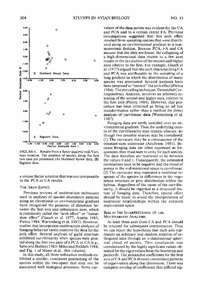
FIGURE 6. Results from a factor analysis with Vari- max rotation. The position of species along the first two axes are presented: (A) Hubbard Brook data, (B) Saguaro data.

a unique factor solution that was not comparable to the PCA or CA results.

THE ARCH Emm

Previous reviews of multivariate techniques used in analyses of species abundance patterns along an elevational or environmental gradient have recognized the presence of distortion between the first axis and subsequent axes, which is commonly called the “arch effect” or “horse- shoe effect” (Gauch et al. 1977, Austin 1985, Pielou 1984, Wartenberg et al. 1987). However, studies that incorporate multivariate analyses of foraging behavior rarely examine the data for the arch effect. Several analyses of guild structure exhibited curvilinearity when species were plotted along the first two axes of a PCA or CA (e.g., Sabo and Holmes 1983; Miles and Ricklefs 1984; and Fig. 1 of Moser et al., this volume).

In this study, all three ordination methods exhibited a similar, consistent positioning of the species within the two-space that may not be associated with biological processes. Some cur-

vature of the data points was evident for the CA and PCA and to a certain extent FA. Previous investigations suggested that this arch effect resulted from sampling species that were distributed along an environmental gradient in a nonmonotonic fashion. Because PCA, FA and CA assume that the data are linear, the collapsing of a high-dimensional data matrix to a few axes results in the involution of the second and higher axes relative to the first. For example, Gauch et al. (1977) argued that the arch characterizing CA and PCA was attributable to the sampling of a long gradient in which the distribution of many species was attenuated. Several methods have been proposed to “correct” the arch effect (Pielou 1984). The prevailing technique, Detrended Cor- respondence Analysis, involves an arbitrary re- scaling of the second and higher axes, relative to the first axis (Pielou 1984). However, this procedure has been criticized as being an ad hoc transformation rather than a method for direct analysis of curvilinear data (Wartenberg et al. 1987).

Foraging data are rarely sampled over an environmental gradient. Thus the underlying caus- es of the curvilinearity may remain obscure, although two possible sources may be considered: (1) The curvature may be a consequence of the constant-sum constraint (Aitchison 198 1). Be- cause foraging data are often expressed as frequencies, they must sum to unity for each species. The data therefore are restricted to lie between the values 0 and 1. Consequently, the estimated correlations tend to be negative and the cloud of points in the n-dimensional space is curvilinear. (2) The curvature may represent a nonlinear re- sponse of the species to differences in the vege- tation structure or prey distribution within the habitat. Regardless of the cause of the curvilinearity, it should be regarded as a structural fea- ture of foraging data. Therefore, special effort should be made to avoid the interpretation of nonlinear relationships within the reduced multivariate space.

BIAS IN THE INTERPRETATION OF THE MULTIVARIATE ANALYSES

At least three axes from CA and PCA should be retained for subsequent interpretation. Thus we can reject the hypothesis that each axis represents an arbitrary and random rotation of orthogonal axes through an n-dimensional spherical cloud of points. This conclusion was corroborated by the highly significant values ob- tained for the eigenvalues from the bootstrap and jackknife. The jackknifed coefficients for the first axis of CA and PCA showed concordant patterns of organization along that dimension. There was complete overlap of coefficients that differed sig-


TABLE 3. COMPARISON OF THE RESULTS FROM THE THREE MULTIVARIATE ANALYSES. THE COEF~CIENTS PRE- SENTED BELOW ARE (1) THE SCORES FOR EACH OF THE 15 VARIABLES FROM A CA, (2) THE NORMALIZED LOADINGS FROM A PCA; AND (3) THE ROTATED FACTOR LOADINGS TOM FA. ANALYSES WERE BALED ON THE SANTA RITA DATA

Variable’ CA

Axis I

PCA FA

Coefficients

Axis 2 Axis 3

CA PCA FA CA PCA FA

GLLF 0.37 -0.210 -0.698 0.85 -0.424 -0.260 0.11 0.119 -0.421 GLTW 0.48 -0.247 -0.705 0.69 -0.33 1 -0.275 0.07 0.135 -0.253 GLBR 0.47 -0.248 -0.577 0.32 -0.099 -0.176 -0.34 0.086 -0.068 GLTR 0.65 -0.188 -0.108 -0.52 0.297 -0.130 -1.11 -0.084 0.321 GLGR 0.00 -0.072 0.069 -0.33 0.159 -0.130 -2.36 -0.222 -0.080 PRBR 1.56 -0.183 -0.043 -1.78 0.455 -0.093 0.37 0.154 0.984 PRTR 1.53 -0.185 -0.048 -1.74 0.449 -0.098 0.34 0.145 0.960 PRGR 1.43 -0.169 -0.093 -1.59 0.384 -0.055 0.06 0.157 0.834 SATW - 1.09 0.294 0.756 -0.45 0.085 0.125 -0.17 -0.305 -0.241 SABR -1.41 0.320 0.926 -0.64 0.079 -0.018 0.13 -0.386 -0.187 HAWK -1.25 0.296 0.798 -0.52 0.064 0.045 -0.02 -0.312 -0.186 HVLF -0.64 0.316 0.069 0.08 -0.040 0.879 0.62 0.356 -0.179 HVTW -1.24 0.335 0.131 -0.40 0.051 0.958 1.10 0.388 -0.039 HVBR - 1.04 0.351 0.333 -0.23 0.013 0.722 0.72 0.203 -0.129 HVTR -0.91 0.289 0.058 -0.50 0.086 0.933 1.00 0.419 0.057

a Codes are: GLLF, glean at IeaS GLTW, glean at twig; GLBR, glean at branch; GLTR, glean at trunk; GLGR, glean at ground, PRBR, probe at branch; PRTR, probe at trunk; PRGR, probe at ground; SATW, sally from twig; SABR, sally from branch, HAWK, aerial manueve~: HVLF, hover at leaf; HVTW, hover at twig; HVBR, hover at branch, and HVTR, hover at trunk.

nificantly from zero. Thus both analyses arrived at a similar group of variables that structured the foraging behavior of species within the community. However, the second and third axes tended to exhibit unique patterns of variation specific to each analysis, -but overlap in the categories that were significant remained relatively high. Most importantly, the results from the jackknife and bootstrap analyses reinforced the in-

terpretations from an analysis ofthe original San- ta Rita data set.

The disparity between PCA and CA in the number of variables that were significantly different from zero in the last two axes may in part be a consequence of the difference in the scaling of the eigenvectors. Because each eigenvector from a PCA is normalized (i.e., the square of the eigenvector equals 1 .O), the coefficients are less

TABLE 4. AN ANALYSIS OF THE DEGREE OF CONCORDANCE OF LOADINGS AMONG THE THREE ORDINATION TECHNIQUES. THE ANALYSIS Is BASED ON KENDALL’S RANK ORDER CORRELATION COEFFICIENT

CA with

Comparison

Sample Axis PCA FA PC-A with FA

Mt. Moosilauke I 0.26 -0.18 0.76*** II 0.55** -0.38 -0.62**

III 0.24 0.28 -0.29

Hubbard Brook I 0.74** 0.67** 0.76** II -0.65** -0.08 0.34

III -0.60** -0.24 0.18 Purica I -0.62** -0.44* 0.67**

II 0.03 -0.73** -0.14 III 0.38 0.17 0.38

Santa Rita I -0.75** -0.55** 0.74** II -0.90*** -0.08 0.03

III 0.76** 0.12 0.28

Saguaro I -0.78** -0.60** 0.73** II -0.77** -0.77** 0.83**

III 0.87*** 0.61** 0.81***

*P < 0.05, **p < 0.01, ***p < 0.001.


TABLE 5. JACKKNIFED CORRFSFQNDENCE ANALYSIS OF THE SANTA RITA DATA. VALUE?, ARE COEFFICIENTS OF THE FIRST THREE EIGENVECXORS (COEFF.), THEIR STANDARD ERRORS (SE), AND THE ERROR RATIOS (ER = COEFF./SE). ESTIMATES OF THE FIRST THREE EIGENVALUES ARE GIVEN AT THE BOTTOM OF EACH COLUMN

Variable

Axis I Axis II Axis III

COEFF. SE ER COEW. SE ER COEF’F. SE ER

GLLF 0.778 0.161 GLTW 0.98 1 0.160 GLBR 0.962 0.135 GLTR 0.557 0.134 GLGR 0.037 0.109 PRBR 0.984 0.462 PRTR 1.047 0.432 PRGR 0.436 0.515 SATW -1.721 0.162 SABR -2.673 0.201 HAWK -1.816 0.167 HVLF -0.946 0.140 HVTW -1.639 0.172 HVBR -1.727 0.137 HVTR - 1.021 0.107

Eigenvalue 0.753 0.019

4.94 6.11 7.09 4.14 0.34 2.12 2.41 0.85

10.60 13.32 10.87 6.74 9.55

12.64 9.48

38.83

0.943 0.103 9.18 0.267 0.063 4.27 0.745 0.149 4.98 0.144 0.084 1.71 0.413 0.196 2.09 - 1.467 0.095 15.49

-0.836 0.175 4.76 -1.299 0.254 5.11 0.255 0.203 1.25 -4.597 0.427 10.71

-3.117 0.374 8.34 0.267 0.187 1.43 -3.161 0.337 9.35 0.405 0.144 3.63 -2.119 0.457 4.63 -0.942 0.259 3.62 -0.134 0.199 0.67 -0.105 0.063 1.66 -0.138 0.287 0.48 0.576 0.162 3.55 -0.032 0.244 1.29 0.296 0.094 3.14

0.331 0.179 1.85 0.097 0.25 1 0.36 0.538 0.232 2.30 0.153 0.447 0.34 0.048 0.255 0.19 0.172 0.223 0.77

-1.772 0.52 3.43 0.201 0.458 0.44

0.829 0.045 18.43 0.329 0.025 10.26

than one by definition. Hence, they tend to have lower standard errors and consequently higher error ratios. However, the magnitude of the coefficients in CA depends on the degree to which the species employs each category; the longer the gradient (i.e., various species specialize on certain foraging categories and therefore recognize each category as distinct), the greater the values for each coefficient. In short, the coefficients are not required to be less than one. This results in higher standard errors and lower error ratios.

Suprisingly, the jackknife estimates of the rotated factor loadings produced rather poor re-

sults. While the results based on the eigenvalues suggested that at least three axes should be retained, estimates of the coefficients were highly biased. Because the coefficients from the jackknife analysis exceeded 1 .O, it is difficult to eval- uate the confidence one should place on an analysis using all data points. The pattern shown in the jackknifed values presented in Table 7 was not unique to the Santa Rita data. Similar trends were evident in all five of the jackknifed factor analyses. Thus, it is possible to discount any artifact due to the data. Most probably, the inflated parameter estimates were a consequence of the

TABLE 6. JACKKNIFED PRINCIPAL COMPONENT ANALYSIS OF THE SANTA RITA DATA. VALUES ARE COEFFICIENTS OF THE FIRST THREE EIGENVECTORS (COEFF.), THEIR ESTIMATED STANDARD ERRORS (SE), AND THE ERROR RATIOS (ER = C0EFF.k). ESTIMATES OF THE FIRST THREE EIGENVALUEZS ARE GIVEN AT THE BOWOM OF EACH COLUMN

Variable


COEF’F. SE ER COEF’F. SE ER COEFF. SE ER

GLLF -0.398 0.039 10.14 -0.449 0.032 13.96 0.026 0.108 0.92 GLTW -0.403 0.027 14.81 -0.347 0.039 9.01 0.130 0.029 4.47 GLBR -0.29 1 0.026 11.29 -0.056 0.066 0.84 0.102 0.033 3.06 GLTR -0.149 0.032 4.65 0.591 0.041 14.35 0.438 0.131 3.35 GLGR -0.042 0.017 2.37 0.257 0.032 7.95 0.445 0.116 3.82 PRBR -0.040 0.036 1.12 0.606 0.029 20.62 -0.570 0.171 3.32 PRTR -0.039 0.033 1.17 0.595 0.03 1 18.93 0.139 0.036 3.87 PRGR 0.004 0.038 0.13 0.345 0.038 8.89 0.188 0.044 4.33 SATW 0.314 0.017 18.07 -0.007 0.032 0.23 -0.382 0.040 9.45 SABR 0.369 0.025 14.77 -0.070 0.043 1.62 -0.884 0.096 9.17 HAWK 0.324 0.031 10.34 -0.074 0.036 2.01 -0.618 0.059 10.46 HVLF 0.415 0.033 12.45 -0.016 0.012 1.25 0.628 0.054 11.58 HVTW 0.378 0.022 17.10 -0.164 0.035 4.72 0.711 0.048 14.68 HVBR 0.391 0.018 20.74 -0.186 0.032 5.85 0.072 0.053 1.36 HVTR 0.322 0.032 10.21 -0.163 0.052 3.18 0.919 0.065 14.08

Eigenvalue 3.425 0.217 15.71 2.263 0.153 14.81 2.388 0.157 15.19


TABLE 7. JACKKNIFED FACTOR ANALYSIS OF THE SANTA RITA DATA. VALUES ARE COEFFICIENTS OF THE FIRST THREE EIGENVEC~OR~ (COEFF.), THEIR ESTIMATED STANDARD ERRORS (SE), AND THE ERROR RATIOS (ER = COEFFJSE)

Variable


COEF'F. SE ER COEFF. SE ER COEFF. SE ER

GLLF -2.181 0.178 12.23 1.242 0.148 8.37 -0.299 0.145 2.06 GLTW -2.841 0.213 13.31 0.301 0.124 2.41 0.186 0.127 1.46 GLBR -2.926 0.225 12.99 0.163 0.136 1.19 0.163 0.136 1.19 GLTR 0.763 0.191 3.99 0.623 0.082 7.63 0.622 0.08 1 7.63 GLGR -0.097 0.028 3.43 -0.146 0.03 1 4.67 -0.145 0.03 1 4.67 PRBR 1.875 0.297 6.30 3.167 0.387 8.17 3.167 0.387 8.18 PRTR 1.818 0.298 6.27 3.076 0.376 8.17 3.076 0.377 8.17 PRGR 1.121 0.257 4.34 3.076 0.363 8.48 3.076 0.363 8.48 SATW 2.922 0.268 10.90 -1.326 0.230 5.76 -1.326 0.230 5.76 SABR 4.617 0.372 12.40 2.276 0.296 7.70 2.276 0.296 7.70 HAWK 3.905 0.330 11.82 -1.973 0.231 8.54 - 1.974 0.231 8.54 HVLF -2.391 0.308 7.77 4.881 0.354 13.78 -3.616 0.395 9.16 HVTW -1.977 0.337 5.85 5.781 0.417 13.83 -3.185 0.377 8.45 HVBR -0.517 0.218 2.36 3.711 0.263 14.09 -3.722 0.362 10.27 HVTR -3.001 0.317 8.09 5.811 0.418 13.90 -1.537 0.299 5.12

factor analytic procedure, in particular the Vari- max rotation of the factor axes. The factor model emphasizes the importance of partitioning common variance from unique variance among the variables. Each recalculation of the FA based on an iterative deletion of a species from the data matrix may produce a unique representation of the correlation structure, which is specific to the suite of remaining species included in the analysis. Consequently, the factor loadings vary dras- tically among the pseudovalues. Therefore, each recalculation produces dramatic changes in magnitude and sign of the rotated factor loadings, rather than a small deviation by deleting an ob-

servation from the data set. Thus, two conclusions emerge from this analysis: either the jackknife analysis of FA was inappropriate, or the estimates from FA were unique to specific groups of species, or both.

IMPLICATIONS OFTHE PRESENT STUDY AND SUGGESTIONS FOR FUTURE STUDIES

CA is the preferred method of analyzing foraging data based on this study. PCA resulted in a similar interpretation of foraging data, but proved less efficient at recovering most of the original variation in the first five axes. These results parallel the study of Gauch et al. (1977)

TABLE 8. B~~T~TRAPPED PRINCIPAL COMPONENT ANALYSIS OF THE SANTA RITA DATA. VALUES ARE COEFFI- CIENTS OF THE FIRST THREE EIGENVECTORS (COEFF.), THEIR ESTIMATED STANDARD ERRORS (SE), ANLI THE ERROR RATIOS (ER = COEFFISE). ESTIMATES OF THE FIRST THREE EIGENVALIJES ARE GIVEN AT THE BOTTOM OF EACH COLUMN

Variable


COEF'F. SE ER COEFF. SE ER COEF'F. SE ER

GLLF -0.142 0.033 4.24 -0.296 0.038 7.62 0.026 0.189 0.14 GLTW -0.119 0.038 3.13 -0.218 0.034 6.23 0.027 0.05 1 0.61 GLBR -0.052 0.058 0.89 -0.033 0.049 0.66 0.153 0.058 2.61 GLTR -0.001 0.045 0.02 0.208 0.031 6.63 0.171 0.133 2.55 GLGR 0.043 0.016 2.60 0.123 0.044 6.04 0.084 0.133 0.63 PRBR -0.001 0.256 0.00 0.269 0.056 4.78 0.020 0.027 0.74 PRTR -0.001 0.257 0.00 0.307 0.039 6.94 0.044 0.029 1.54 PRGR 0.005 0.069 0.02 0.275 0.041 6.74 0.029 0.022 1.27 SATW 0.137 0.067 1.98 0.093 0.060 3.92 0.009 0.074 0.12 SABR 0.123 0.082 1.49 0.056 0.192 0.29 -0.156 0.059 2.64 HAWK 0.123 0.07 1 1.73 0.040 0.178 0.22 -0.173 0.050 3.44 HVLF 0.147 0.036 4.08 0.063 0.186 0.33 0.263 0.049 5.33 HVTW 0.151 0.056 2.66 0.082 0.128 0.64 0.167 0.06 1 2.73 HVBR 0.140 0.067 2.08 0.038 0.146 0.26 0.116 0.087 1.33 HVTR 0.208 0.031 6.71 0.121 0.020 5.91 0.134 0.059 2.25

Eigenvalue 5.374 0.059 91.34 3.58 0.032 111.03 2.45 1 0.032 75.16


who found that CA produced ordinations of sim- ulated community patterns superior to those from PCA. Several points make compelling the use of CA in foraging studies. It recovers a high amount of the original variation in the data, despite the curvilinear nature of foraging data. A large proportion of jackknifed coefficients from the first three axes were significantly different from zero. In addition, the estimates of the coefficients exhibited low bias (i.e., the observed coefficients fell within f2 SE of the jackknifed coefficient). Thus, the interpretations of the patterns of variation in foraging behavior are not based on an arbitrary rotation of axes through a cloud of points. Finally, the absence of the most commonly cited disadvantage of CA, the compression of species at the terminal portions of each axis, provides additional evidence supporting the use of CA in foraging studies.

Factor analysis of foraging data produced relatively unsatisfactory results. While the amount of variance extracted was similar to PCA, FA exhibited a low degree of correspondence with the results from CA and PCA. The presence of the arch effect after rotation of the axes suggests that extreme caution must be exercised in interpretation of the rotated axes. This is especially true because most rotations involve an orthogonal transformation of the axes, and the deci- sively curvilinear nature of the data may violate the assumptions of the technique. The premise of the FA model-to extract variation from among a group of highly correlated variables after removing the variation attributable to the unique factors-precludes generalizing or comparing results from other studies. This is com- pounded by conducting the analysis on a correlation matrix. Standardization of the variables by their standard deviation distorts the ecological space, and consequently any patterns that emerge are specific to the particular data set and group of species (Miles and Ricklefs 1984). How- ever, the practice of using a correlation matrix must be balanced by the need to use scale-invariant data with PCA and FA. Yet, this argues more forcefully for using CA, because the standardization of the data is not necessary. A ma- jority of the jackknifed coefficients, although significantly different from zero, exceeded 1.0. Between 80 and 100% of the estimated coeffi-

cients were biased. The general conclusion is that FA is inappropriate for the analysis of foraging data.

Further caution must be emphasized in draw- ing generalizations from multivariate analyses. Most foraging data consist of many observations recorded for a small number of species. Often the number of categories is greater than the number of species. The results from CA, PCA and FA calculated with small sample sizes may be highly sensitive to additions or deletions of foraging categories, random variation in foraging behavior, and the presence of empty cells in the data matrix.

ALTERNATIVE MULTIVARIATE METHODS

The three multivariate methods evaluated in this study all assume that the data were approximately linear. While several studies have dem- onstrated that CA is less sensitive to curvilinearities within the data (e.g., Gauch et al. 1977, Pielou 1984) than PCA, any interpretations about underlying patterns will be hindered by the presence of the arch. Consequently, nonparametric multivariate methods should prove to be appropriate alternative modes of analysis. Earlier studies that compared nonparametric methods, in particular nonmetric multidimensional scaling (NM-MDS), with PCA or CA found that the for- mer method extracted pattern with lower distortion due to curvilinearities present in the data (Fasham 1977). Techniques such as NM-MDS, psychophysical unfolding theory, and nonparametric mapping have proven to be effective in describing guild structure (e.g., Adams 1985) and resource axes (Gray 1979, Gray and Ring 1986). Subsequent analyses of avian foraging data should incorporate these underused methods.

ACKNOWLEDGMENTS I thank R. E. Ricklefs and A. E. Dunham for stim-

ulating discussions about various aspects of the analyses. The critical comments of Barry Noon and Jared Vemer greatly clarified many aspects of the manu- script. Peter Landres graciously shared unpublished data. Computer time was provided by Ohio Univer- sity. David Althoffassisted in various stages of the data analysis. Various stages of the research were supported by the Frank M. Chapman Memorial Fund, Sigma Xi, and the Explorers Club. The writing of this research was sponsored in part by NSF grant BSR-86 16788.