Arthur Charpentier, Université de Rennes 1, Portfolio Optimization - 2017
Portfolio Optimization # 2A. Charpentier (Université de Rennes 1)
Université de Rennes 1, 2017/2018
@freakonometrics freakonometrics freakonometrics.hypotheses.org 1
Arthur Charpentier, Université de Rennes 1, Portfolio Optimization - 2017
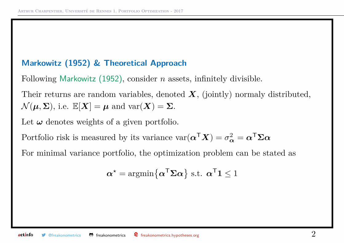
Markowitz (1952) & Theoretical Approach
Following Markowitz (1952), consider n assets, infinitely divisible.
Their returns are random variables, denoted X, (jointly) normaly distributed,N (µ,Σ), i.e. E[X] = µ and var(X) = Σ.
Let ω denotes weights of a given portfolio.
Portfolio risk is measured by its variance var(αTX) = σ2α = αTΣα
For minimal variance portfolio, the optimization problem can be stated as
α? = argmin{αTΣα
}s.t. αT1 ≤ 1
@freakonometrics freakonometrics freakonometrics.hypotheses.org 2
Arthur Charpentier, Université de Rennes 1, Portfolio Optimization - 2017
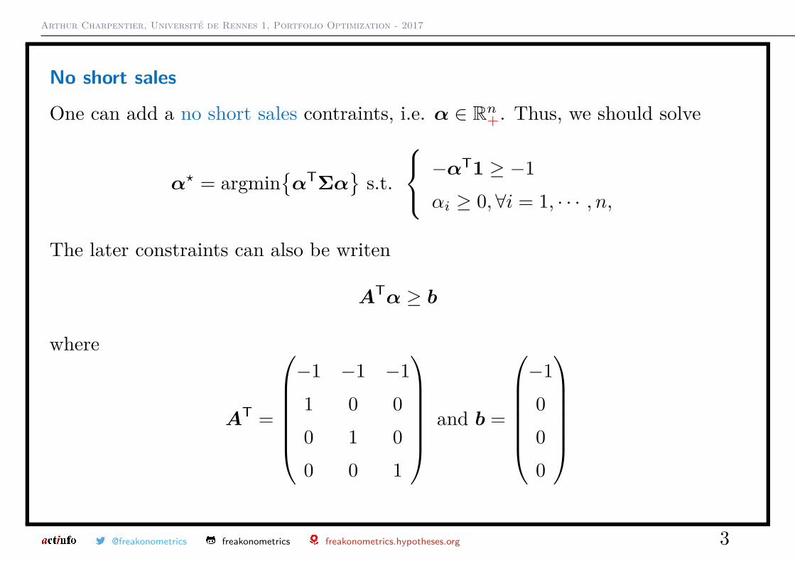
No short sales
One can add a no short sales contraints, i.e. α ∈ Rn+. Thus, we should solve
α? = argmin{αTΣα
}s.t.
−αT1 ≥ −1αi ≥ 0,∀i = 1, · · · , n,
The later constraints can also be writen
ATα ≥ b
where
AT =
−1 −1 −11 0 00 1 00 0 1
and b =
−1000
@freakonometrics freakonometrics freakonometrics.hypotheses.org 3
Arthur Charpentier, Université de Rennes 1, Portfolio Optimization - 2017
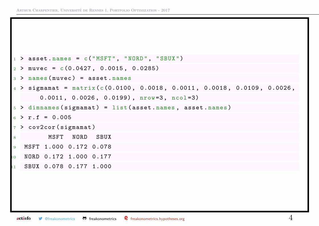
1 > asset . names = c("MSFT", "NORD", "SBUX")
2 > muvec = c(0.0427 , 0.0015 , 0.0285)
3 > names ( muvec ) = asset . names
4 > sigmamat = matrix (c(0.0100 , 0.0018 , 0.0011 , 0.0018 , 0.0109 , 0.0026 ,
0.0011 , 0.0026 , 0.0199) , nrow =3, ncol =3)
5 > dimnames ( sigmamat ) = list( asset .names , asset . names )
6 > r.f = 0.005
7 > cov2cor ( sigmamat )
8 MSFT NORD SBUX
9 MSFT 1.000 0.172 0.078
10 NORD 0.172 1.000 0.177
11 SBUX 0.078 0.177 1.000
@freakonometrics freakonometrics freakonometrics.hypotheses.org 4
Arthur Charpentier, Université de Rennes 1, Portfolio Optimization - 2017
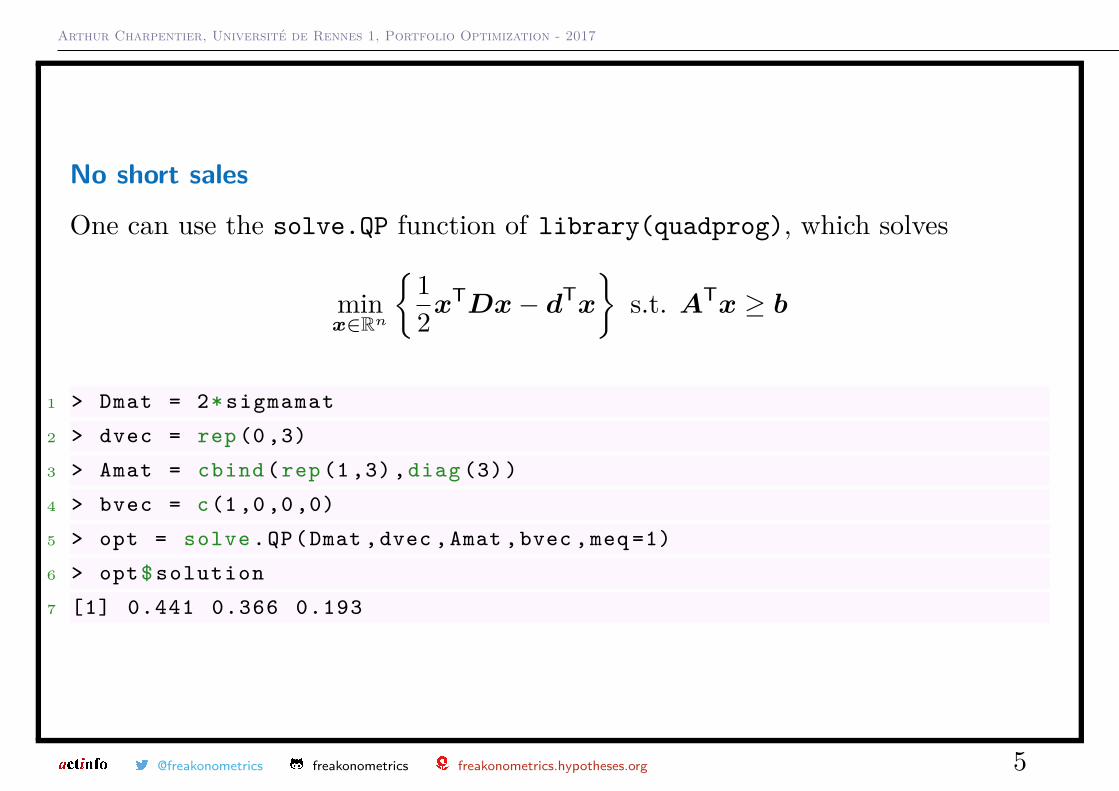
No short sales
One can use the solve.QP function of library(quadprog), which solves
minx∈Rn
{12x
TDx− dTx
}s.t. ATx ≥ b
1 > Dmat = 2* sigmamat
2 > dvec = rep (0 ,3)
3 > Amat = cbind (rep (1 ,3) ,diag (3))
4 > bvec = c(1 ,0 ,0 ,0)
5 > opt = solve .QP(Dmat ,dvec ,Amat ,bvec ,meq =1)
6 > opt$ solution
7 [1] 0.441 0.366 0.193
@freakonometrics freakonometrics freakonometrics.hypotheses.org 5
Arthur Charpentier, Université de Rennes 1, Portfolio Optimization - 2017
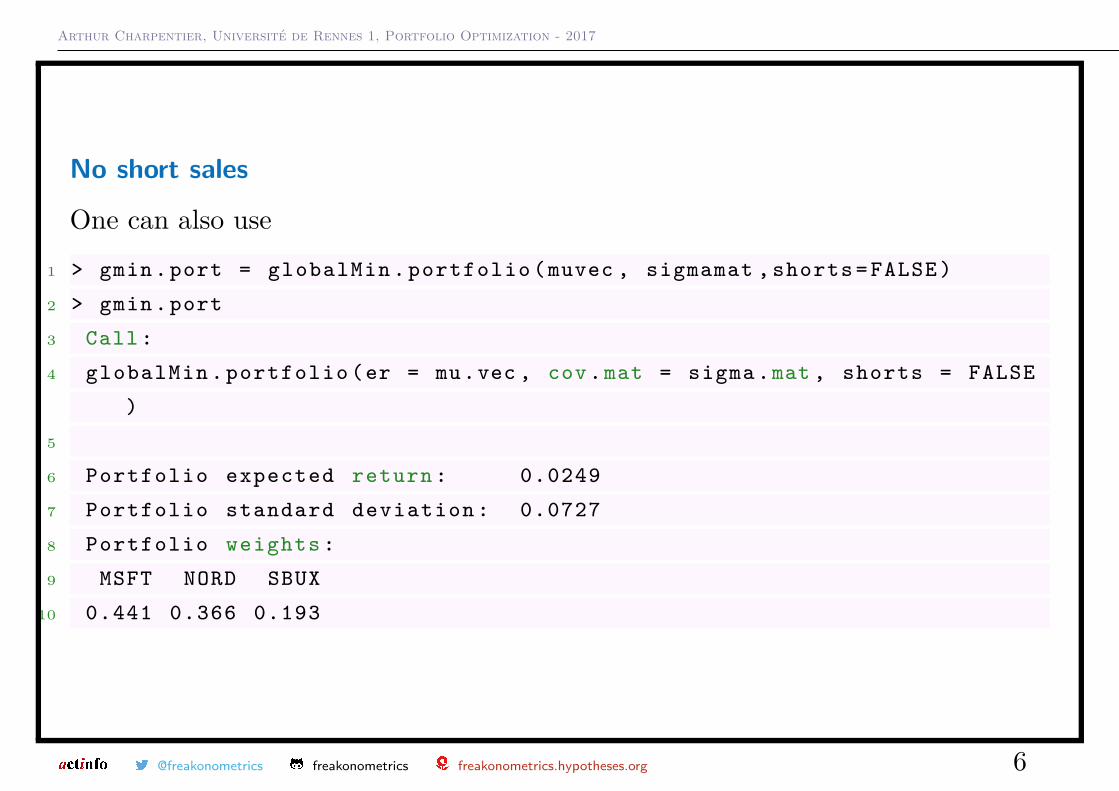
No short sales
One can also use1 > gmin.port = globalMin . portfolio (muvec , sigmamat , shorts = FALSE )
2 > gmin.port
3 Call:
4 globalMin . portfolio (er = mu.vec , cov.mat = sigma .mat , shorts = FALSE
)
5
6 Portfolio expected return : 0.0249
7 Portfolio standard deviation : 0.0727
8 Portfolio weights :
9 MSFT NORD SBUX
10 0.441 0.366 0.193
@freakonometrics freakonometrics freakonometrics.hypotheses.org 6
Arthur Charpentier, Université de Rennes 1, Portfolio Optimization - 2017
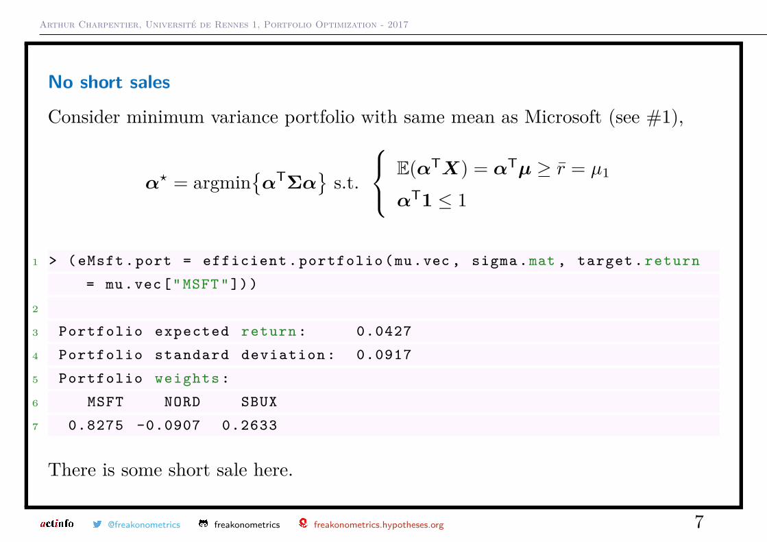
No short sales
Consider minimum variance portfolio with same mean as Microsoft (see #1),
α? = argmin{αTΣα
}s.t.
E(αTX) = αTµ ≥ r̄ = µ1
αT1 ≤ 1
1 > ( eMsft .port = efficient . portfolio (mu.vec , sigma .mat , target . return
= mu.vec["MSFT"]))
2
3 Portfolio expected return : 0.0427
4 Portfolio standard deviation : 0.0917
5 Portfolio weights :
6 MSFT NORD SBUX
7 0.8275 -0.0907 0.2633
There is some short sale here.
@freakonometrics freakonometrics freakonometrics.hypotheses.org 7
Arthur Charpentier, Université de Rennes 1, Portfolio Optimization - 2017
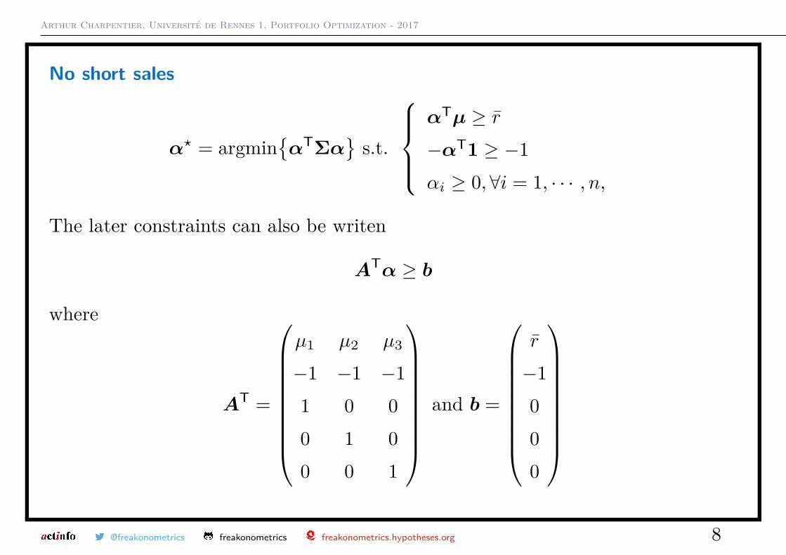
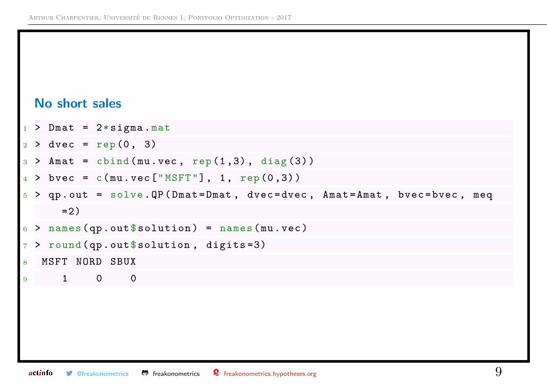
No short sales
α? = argmin{αTΣα
}s.t.
αTµ ≥ r̄−αT1 ≥ −1αi ≥ 0,∀i = 1, · · · , n,
The later constraints can also be writen
ATα ≥ b
where
AT =
µ1 µ2 µ3
−1 −1 −11 0 00 1 00 0 1
and b =
r̄
−1000
@freakonometrics freakonometrics freakonometrics.hypotheses.org 8
Arthur Charpentier, Université de Rennes 1, Portfolio Optimization - 2017
No short sales1 > Dmat = 2* sigma .mat
2 > dvec = rep (0, 3)
3 > Amat = cbind (mu.vec , rep (1 ,3) , diag (3))
4 > bvec = c(mu.vec["MSFT"], 1, rep (0 ,3))
5 > qp.out = solve .QP(Dmat=Dmat , dvec=dvec , Amat=Amat , bvec=bvec , meq
=2)
6 > names (qp.out$ solution ) = names (mu.vec)
7 > round (qp.out$solution , digits =3)
8 MSFT NORD SBUX
9 1 0 0
@freakonometrics freakonometrics freakonometrics.hypotheses.org 9
Arthur Charpentier, Université de Rennes 1, Portfolio Optimization - 2017
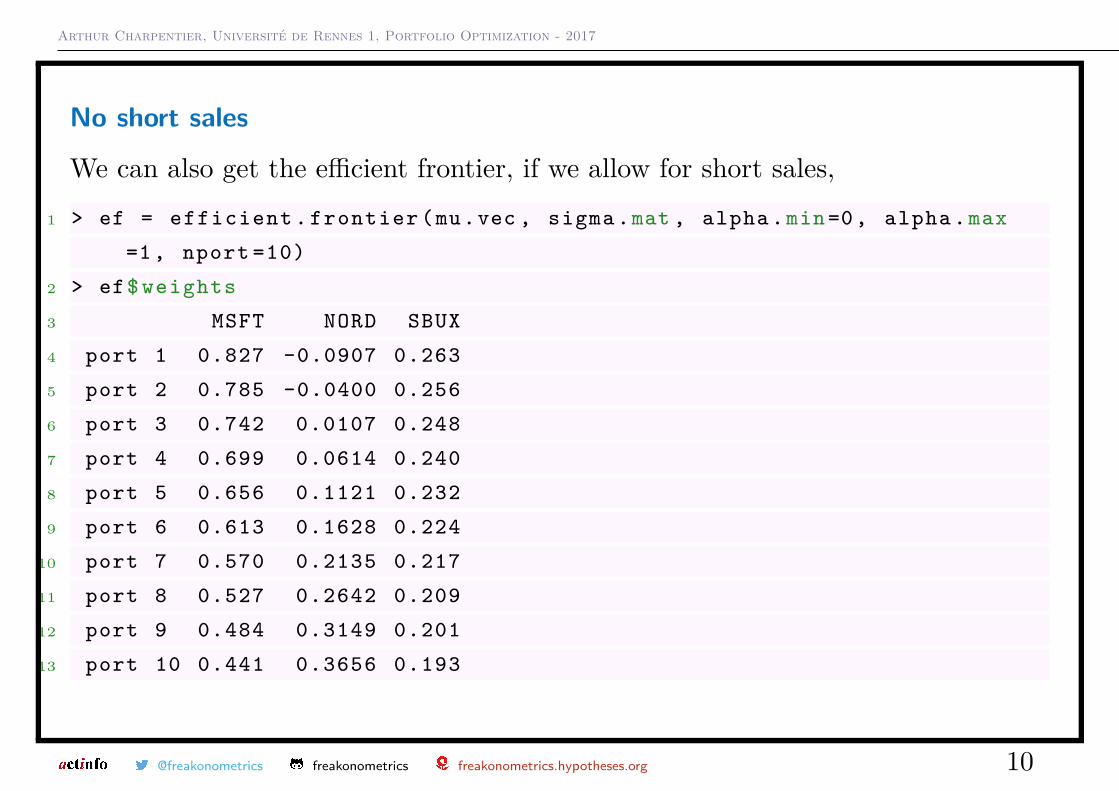
No short sales
We can also get the efficient frontier, if we allow for short sales,1 > ef = efficient . frontier (mu.vec , sigma .mat , alpha .min =0, alpha .max
=1, nport =10)
2 > ef$ weights
3 MSFT NORD SBUX
4 port 1 0.827 -0.0907 0.263
5 port 2 0.785 -0.0400 0.256
6 port 3 0.742 0.0107 0.248
7 port 4 0.699 0.0614 0.240
8 port 5 0.656 0.1121 0.232
9 port 6 0.613 0.1628 0.224
10 port 7 0.570 0.2135 0.217
11 port 8 0.527 0.2642 0.209
12 port 9 0.484 0.3149 0.201
13 port 10 0.441 0.3656 0.193
@freakonometrics freakonometrics freakonometrics.hypotheses.org 10
Arthur Charpentier, Université de Rennes 1, Portfolio Optimization - 2017
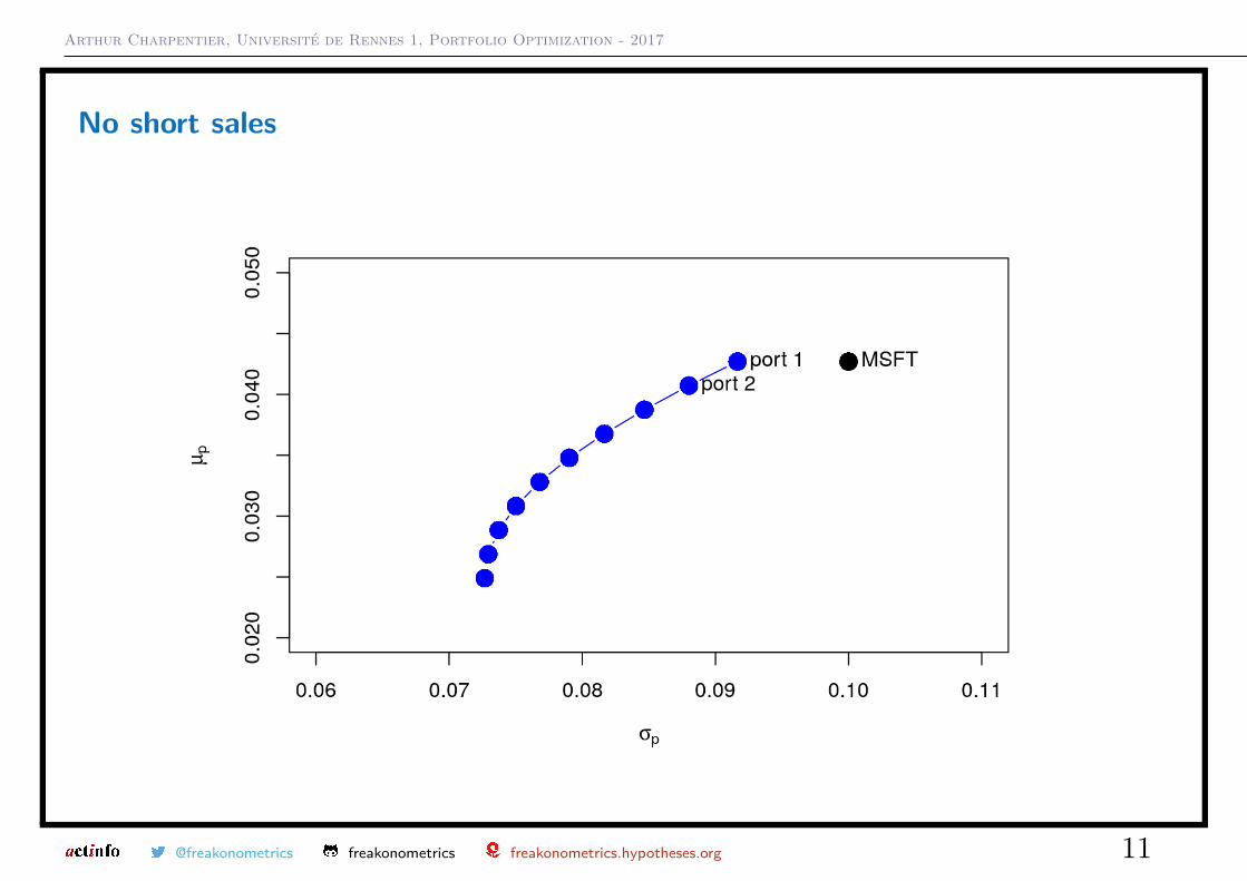
No short sales
@freakonometrics freakonometrics freakonometrics.hypotheses.org 11
Arthur Charpentier, Université de Rennes 1, Portfolio Optimization - 2017
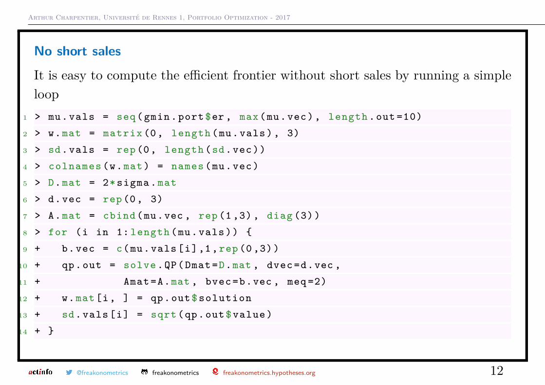
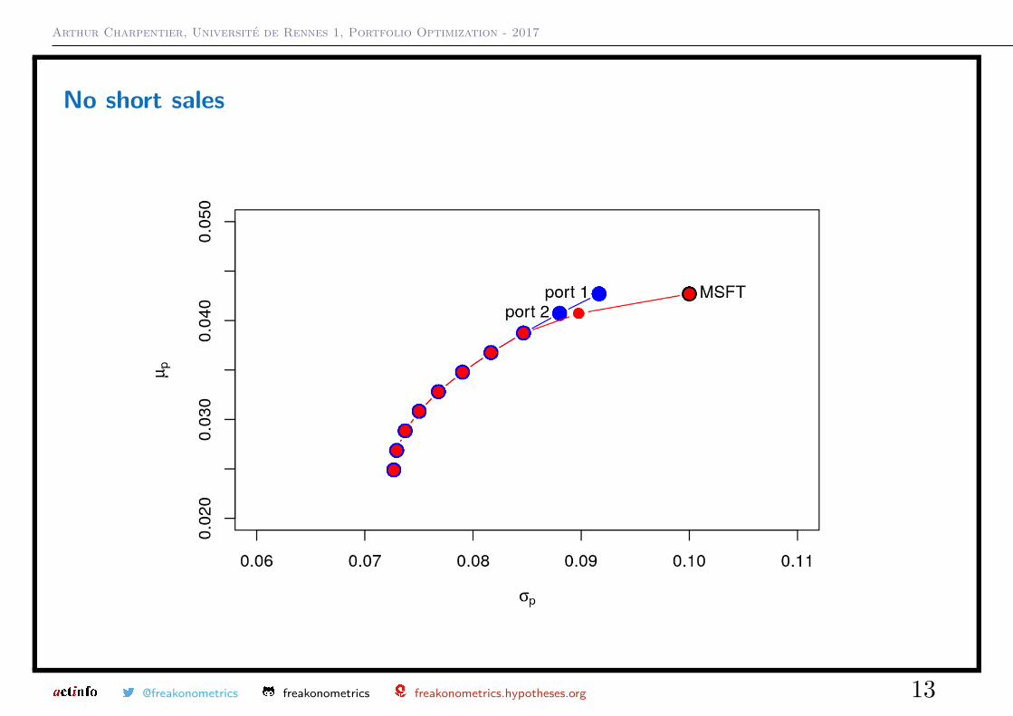
No short sales
It is easy to compute the efficient frontier without short sales by running a simpleloop
1 > mu.vals = seq(gmin.port$er , max(mu.vec), length .out =10)
2 > w.mat = matrix (0, length (mu.vals), 3)
3 > sd.vals = rep (0, length (sd.vec))
4 > colnames (w.mat) = names (mu.vec)
5 > D.mat = 2* sigma .mat
6 > d.vec = rep (0, 3)
7 > A.mat = cbind (mu.vec , rep (1 ,3) , diag (3))
8 > for (i in 1: length (mu.vals)) {
9 + b.vec = c(mu.vals[i],1, rep (0 ,3))
10 + qp.out = solve .QP(Dmat=D.mat , dvec=d.vec ,
11 + Amat=A.mat , bvec=b.vec , meq =2)
12 + w.mat[i, ] = qp.out$ solution
13 + sd.vals[i] = sqrt(qp.out$ value )
14 + }
@freakonometrics freakonometrics freakonometrics.hypotheses.org 12
Arthur Charpentier, Université de Rennes 1, Portfolio Optimization - 2017
No short sales
@freakonometrics freakonometrics freakonometrics.hypotheses.org 13
Arthur Charpentier, Université de Rennes 1, Portfolio Optimization - 2017
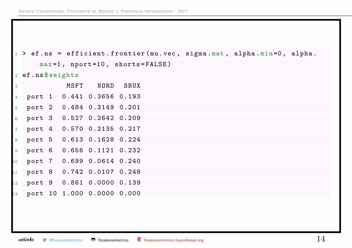
1 > ef.ns = efficient . frontier (mu.vec , sigma .mat , alpha .min =0, alpha .
max =1, nport =10 , shorts = FALSE )
2 ef.ns$ weights
3 MSFT NORD SBUX
4 port 1 0.441 0.3656 0.193
5 port 2 0.484 0.3149 0.201
6 port 3 0.527 0.2642 0.209
7 port 4 0.570 0.2135 0.217
8 port 5 0.613 0.1628 0.224
9 port 6 0.656 0.1121 0.232
10 port 7 0.699 0.0614 0.240
11 port 8 0.742 0.0107 0.248
12 port 9 0.861 0.0000 0.139
13 port 10 1.000 0.0000 0.000
@freakonometrics freakonometrics freakonometrics.hypotheses.org 14
Arthur Charpentier, Université de Rennes 1, Portfolio Optimization - 2017
@freakonometrics freakonometrics freakonometrics.hypotheses.org 15
Arthur Charpentier, Université de Rennes 1, Portfolio Optimization - 2017
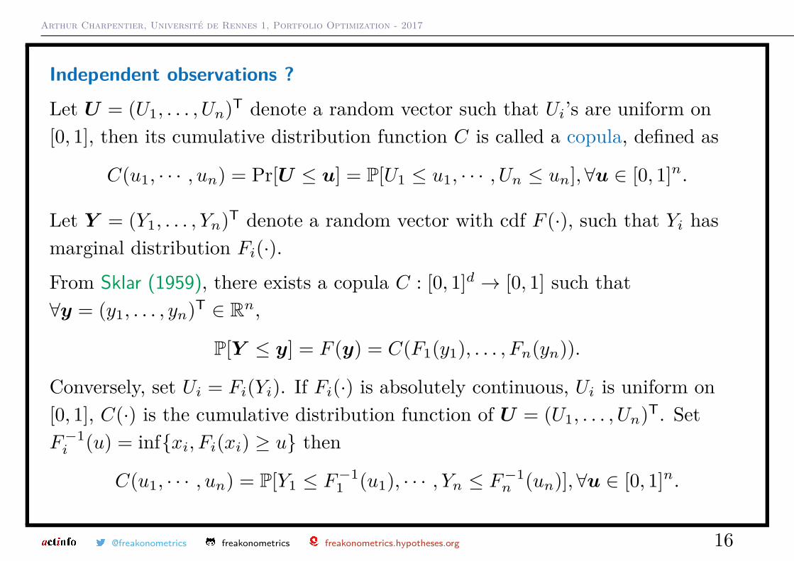
Independent observations ?
Let U = (U1, . . . , Un)T denote a random vector such that Ui’s are uniform on[0, 1], then its cumulative distribution function C is called a copula, defined as
C(u1, · · · , un) = Pr[U ≤ u] = P[U1 ≤ u1, · · · , Un ≤ un],∀u ∈ [0, 1]n.
Let Y = (Y1, . . . , Yn)T denote a random vector with cdf F (·), such that Yi hasmarginal distribution Fi(·).
From Sklar (1959), there exists a copula C : [0, 1]d → [0, 1] such that∀y = (y1, . . . , yn)T ∈ Rn,
P[Y ≤ y] = F (y) = C(F1(y1), . . . , Fn(yn)).
Conversely, set Ui = Fi(Yi). If Fi(·) is absolutely continuous, Ui is uniform on[0, 1], C(·) is the cumulative distribution function of U = (U1, . . . , Un)T. SetF−1i (u) = inf{xi, Fi(xi) ≥ u} then
C(u1, · · · , un) = P[Y1 ≤ F−11 (u1), · · · , Yn ≤ F−1
n (un)],∀u ∈ [0, 1]n.
@freakonometrics freakonometrics freakonometrics.hypotheses.org 16
Arthur Charpentier, Université de Rennes 1, Portfolio Optimization - 2017
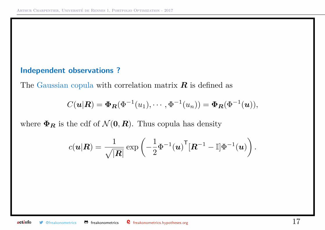
Independent observations ?
The Gaussian copula with correlation matrix R is defined as
C(u|R) = ΦR(Φ−1(u1), · · · ,Φ−1(un)) = ΦR(Φ−1(u)),
where ΦR is the cdf of N (0,R). Thus copula has density
c(u|R) = 1√|R|
exp(−1
2Φ−1(u)T[R−1 − I]Φ−1(u)).
@freakonometrics freakonometrics freakonometrics.hypotheses.org 17
Arthur Charpentier, Université de Rennes 1, Portfolio Optimization - 2017
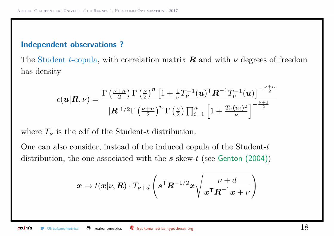
Independent observations ?
The Student t-copula, with correlation matrix R and with ν degrees of freedomhas density
c(u|R, ν) =Γ(ν+n
2)
Γ(ν2)n [1 + 1
νT−1ν (u)TR−1T−1
ν (u)]− ν+n
2
|R|1/2Γ(ν+n
2)n Γ
(ν2)∏n
i=1
[1 + Tν(ui)2
ν
]− ν+12
where Tν is the cdf of the Student-t distribution.
One can also consider, instead of the induced copula of the Student-tdistribution, the one associated with the s skew-t (see Genton (2004))
x 7→ t(x|ν,R) · Tν+d
(sTR−1/2x
√ν + d
xTR−1x+ ν
)
@freakonometrics freakonometrics freakonometrics.hypotheses.org 18
Arthur Charpentier, Université de Rennes 1, Portfolio Optimization - 2017
@freakonometrics freakonometrics freakonometrics.hypotheses.org 19
Arthur Charpentier, Université de Rennes 1, Portfolio Optimization - 2017
Independent Return ?
It might be more realistic to consider the conditional distribution of Y t giveninformation Ft−1.
Assume that Y t has conditional distribution F (·|Ft−1), such that ∀i, Yi,t hasconditional distribution Fi(·|Ft−1).
There exists C(·|Ft−1) : [0, 1]d → [0, 1] such that ∀y = (y1, . . . , yn)T ∈ Rn,
P[Y t ≤ y|Ft−1] = F (y|Ft−1) = C(F1(y1|Ft−1), . . . , Fn(yn|Ft−1)|Ft−1).
Conversely, set Ui,t = Fi(Yi,t|Ft−1). If Fi(·|Ft−1) is absolutely continuous,C(·|Ft−1) is the cdf of U t = (U1,t, . . . , Ud,t)T, given Ft−1.
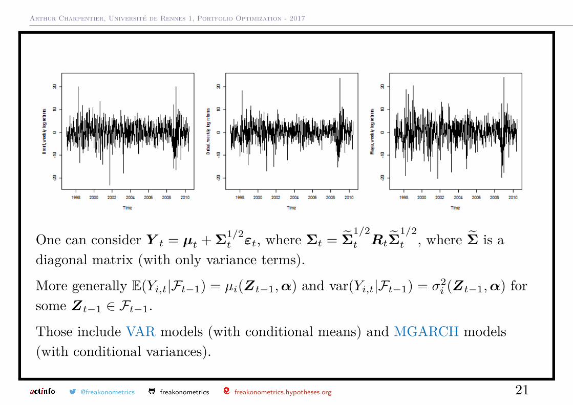
Consider weekly returns of oil prices, Brent, Dubaï and Maya.
@freakonometrics freakonometrics freakonometrics.hypotheses.org 20
Arthur Charpentier, Université de Rennes 1, Portfolio Optimization - 2017
One can consider Y t = µt + Σ1/2t εt, where Σt = Σ̃
1/2t RtΣ̃
1/2t , where Σ̃ is a
diagonal matrix (with only variance terms).
More generally E(Yi,t|Ft−1) = µi(Zt−1,α) and var(Yi,t|Ft−1) = σ2i (Zt−1,α) for
some Zt−1 ∈ Ft−1.
Those include VAR models (with conditional means) and MGARCH models(with conditional variances).
@freakonometrics freakonometrics freakonometrics.hypotheses.org 21
Arthur Charpentier, Université de Rennes 1, Portfolio Optimization - 2017
VAR models
See Sims (1980) and Lütkepohl (2007)
E(Yi,t|Ft−1) = µi,0 + µi(Y t−1,Φ,Σ) = ΦTi Y t−1,
andvar(Yi,t|Ft−1) = σ2
i (Y t−1,Φ,Σ) = Σi,i.
Or fit univariate models,1 > fit1 = arima (x=dat [,1], order =c(2 ,0 ,1))
2 > library ( fGarch )
3 > fit1 = garchFit ( formula = ~ arma (2 ,1)+ garch (1, 1) ,data=dat [,1], cond
.dist ="std",trace = FALSE )
@freakonometrics freakonometrics freakonometrics.hypotheses.org 22
Arthur Charpentier, Université de Rennes 1, Portfolio Optimization - 2017
MGARCH models
See Engle & Kroner (1995) for the BEEK model
Consider Y t = Σ1/2t εt where E(εt) = 0 and var(εt) = I.
The MGARCH(1,1) is defined as
Σt = ωTω +ATεt−1εTt−1A+BTΣt−1B
where ω, A et B are d× d matrices (ω can be triangular matrix). Then
E(Yi,t|Ft−1) = µi(Σt−1, εt−1,ω,A,B,Σ) = 0
and Σt = V (Y t|Ft−1) with
var(Yi,t|Ft−1) = σ2i (Σt−1, εt−1,ω,A,B,Σ) = Σi,i,t
i.e.var(Yi,t|Ft−1) = ωT
i ωi +ATi εt−1ε
Tt−1Ai +BT
i Σt−1Bi.
@freakonometrics freakonometrics freakonometrics.hypotheses.org 23
Arthur Charpentier, Université de Rennes 1, Portfolio Optimization - 2017
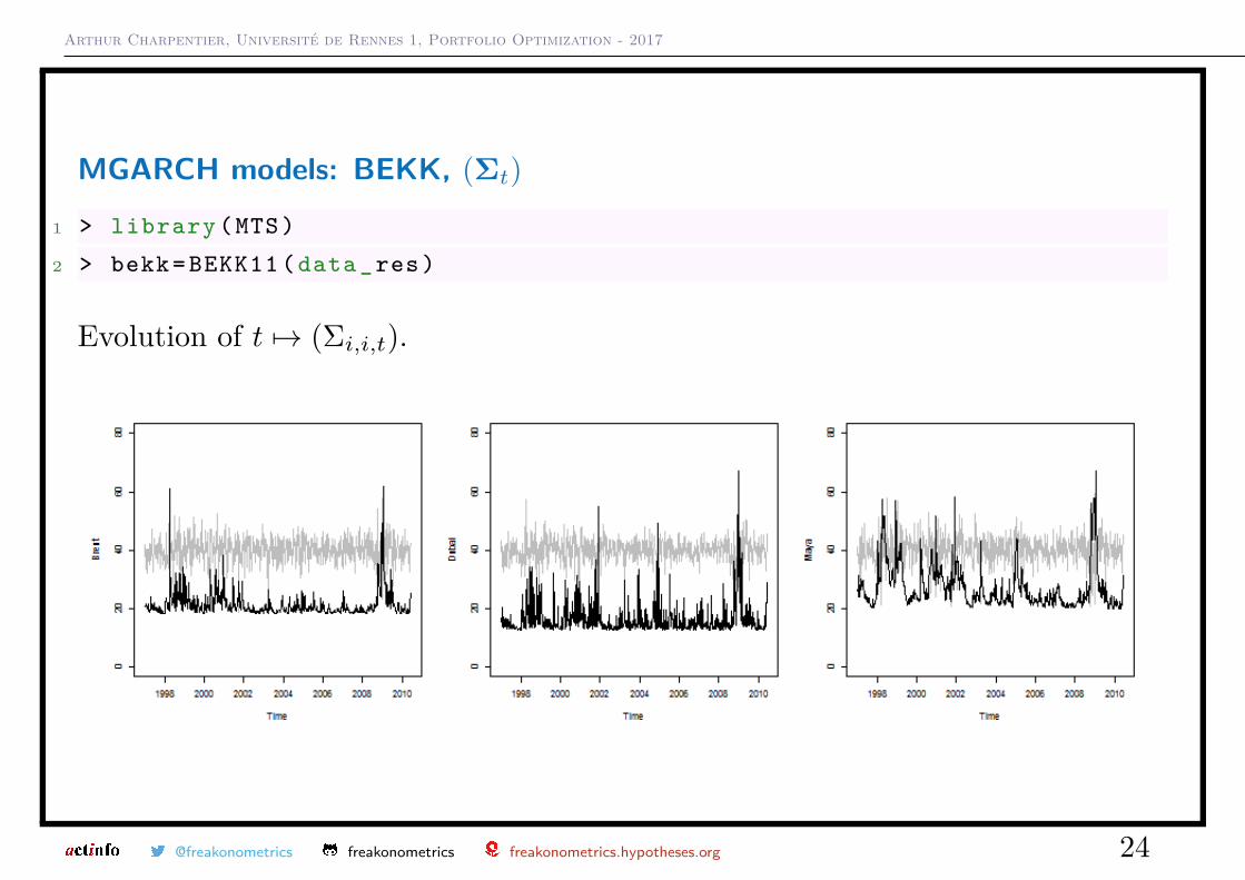
MGARCH models: BEKK, (Σt)
1 > library (MTS)
2 > bekk= BEKK11 (data_res)
Evolution of t 7→ (Σi,i,t).
@freakonometrics freakonometrics freakonometrics.hypotheses.org 24
Arthur Charpentier, Université de Rennes 1, Portfolio Optimization - 2017
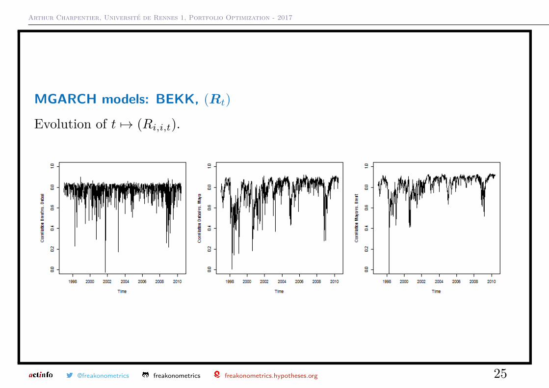
MGARCH models: BEKK, (Rt)
Evolution of t 7→ (Ri,i,t).
@freakonometrics freakonometrics freakonometrics.hypotheses.org 25
Arthur Charpentier, Université de Rennes 1, Portfolio Optimization - 2017
Copula based models
Here Yi,t = µi(Zt−1,α) + σi(Zt−1,α) · εi,t, thus, define standardized residuals
εi,t = Yi,t − µi(Zt−1,α)σi(Zt−1,α) .
Recall that the (conditional) correlation matrix is Rt = Σ̃−1/2t ΣtΣ̃
−1/2t , where
Σ̃t = diag(Σt), with
Ri,j,t = cor(εi,t, εj,t|Ft−1) = E[εi,tεj,t|Ft−1].
Engle (2002) suggested Rt = Q̃−1/2t QtQ̃
−1/2t where Qt is driven by
Qt = [1− α− β]Q+ αQt−1 + βεt−1εTt−1,
where Q is the unconditional variance of (ηt), and where coefficients α and β arepositive, with α+ β ∈ (0, 1).
@freakonometrics freakonometrics freakonometrics.hypotheses.org 26
Arthur Charpentier, Université de Rennes 1, Portfolio Optimization - 2017
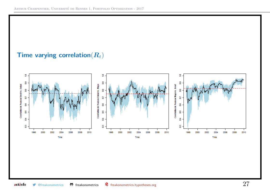
Time varying correlation(Rt)
@freakonometrics freakonometrics freakonometrics.hypotheses.org 27
Arthur Charpentier, Université de Rennes 1, Portfolio Optimization - 2017
EWMA : Exponentially Weighted Moving Average
In the univariate case,
σ2t = (1− λ)[rt−1 − µt−1]2 + λσ2
t−1,
with λ ∈ [0, 1). It is called Exponentially Weighted Moving Average because
σ2t = [1− λ]
n∑i=1
λiσ2t−i + λnσ2
t−n︸ ︷︷ ︸ = [1− λ]∞∑i=1
λiσ2t−i.
The (natural) multivariate extention would be
Σt = (1− λ)(rt−1 − µt−1)(rt−1 − µt−1)T + ΛΣt−1,
in the sense that
Σi,j,t = (1− λ)[ri,t−1 − µi,t−1][rj,t−1 − µj,t−1] + λΣi,j,t−1
see Lowry et al. (1992).
@freakonometrics freakonometrics freakonometrics.hypotheses.org 28
Arthur Charpentier, Université de Rennes 1, Portfolio Optimization - 2017
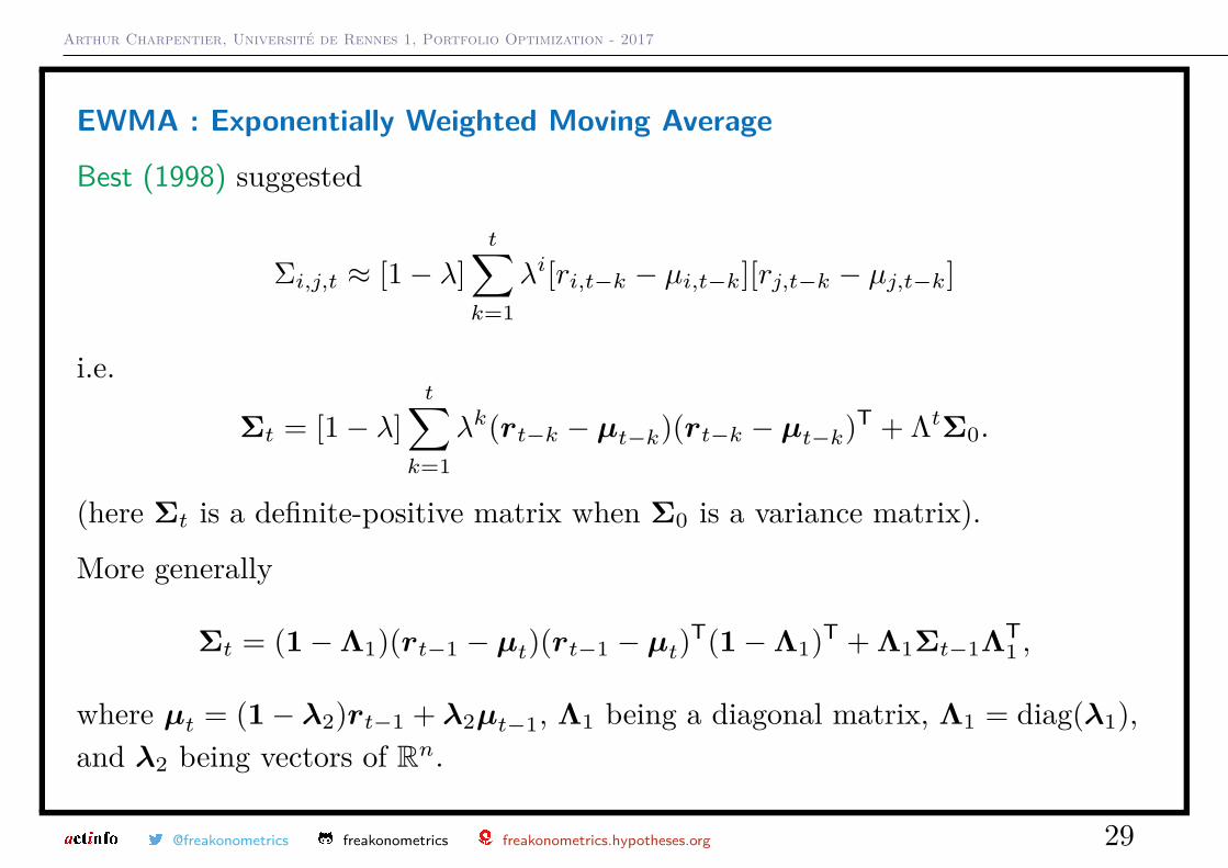
EWMA : Exponentially Weighted Moving Average
Best (1998) suggested
Σi,j,t ≈ [1− λ]t∑
k=1λi[ri,t−k − µi,t−k][rj,t−k − µj,t−k]
i.e.
Σt = [1− λ]t∑
k=1λk(rt−k − µt−k)(rt−k − µt−k)T + ΛtΣ0.
(here Σt is a definite-positive matrix when Σ0 is a variance matrix).
More generally
Σt = (1−Λ1)(rt−1 − µt)(rt−1 − µt)T(1−Λ1)T + Λ1Σt−1ΛT1 ,
where µt = (1− λ2)rt−1 + λ2µt−1, Λ1 being a diagonal matrix, Λ1 = diag(λ1),and λ2 being vectors of Rn.
@freakonometrics freakonometrics freakonometrics.hypotheses.org 29
Arthur Charpentier, Université de Rennes 1, Portfolio Optimization - 2017
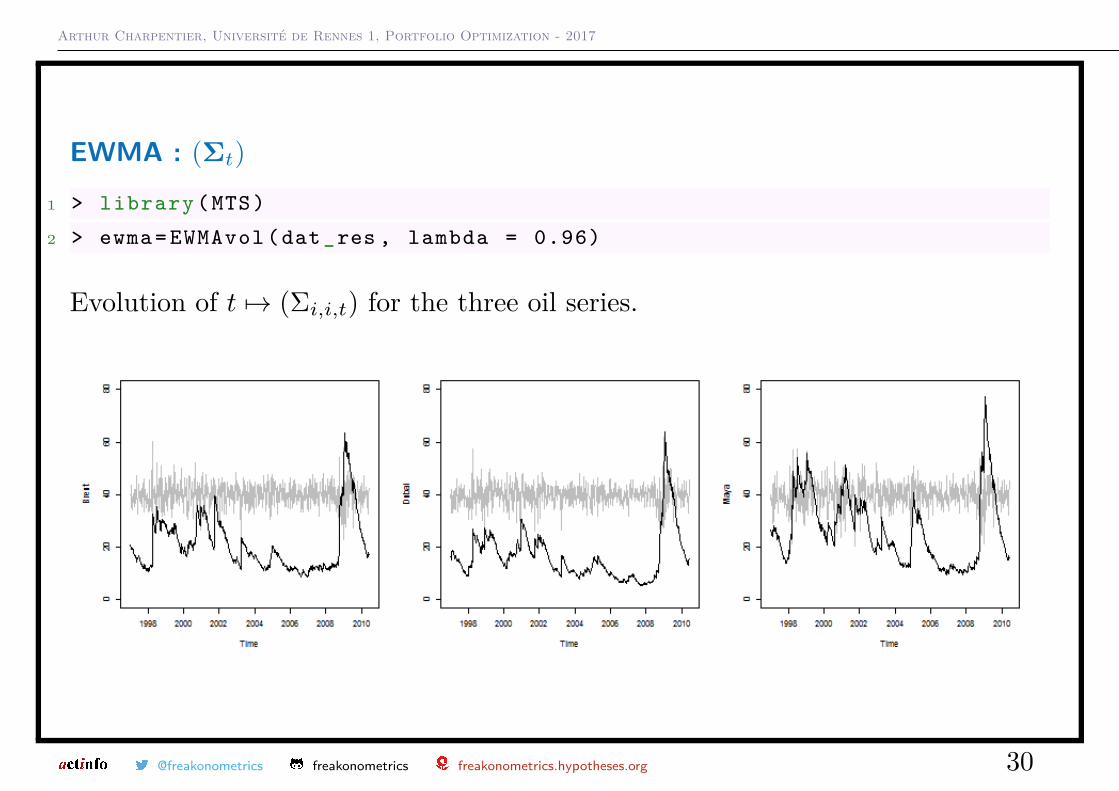
EWMA : (Σt)
1 > library (MTS)
2 > ewma= EWMAvol (dat_res , lambda = 0.96)
Evolution of t 7→ (Σi,i,t) for the three oil series.
@freakonometrics freakonometrics freakonometrics.hypotheses.org 30
Arthur Charpentier, Université de Rennes 1, Portfolio Optimization - 2017
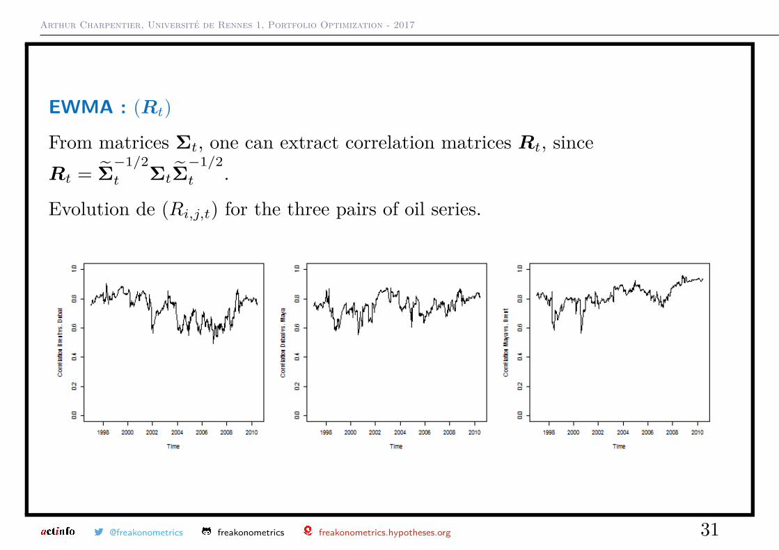
EWMA : (Rt)
From matrices Σt, one can extract correlation matrices Rt, sinceRt = Σ̃
−1/2t ΣtΣ̃
−1/2t .
Evolution de (Ri,j,t) for the three pairs of oil series.
@freakonometrics freakonometrics freakonometrics.hypotheses.org 31
Arthur Charpentier, Université de Rennes 1, Portfolio Optimization - 2017
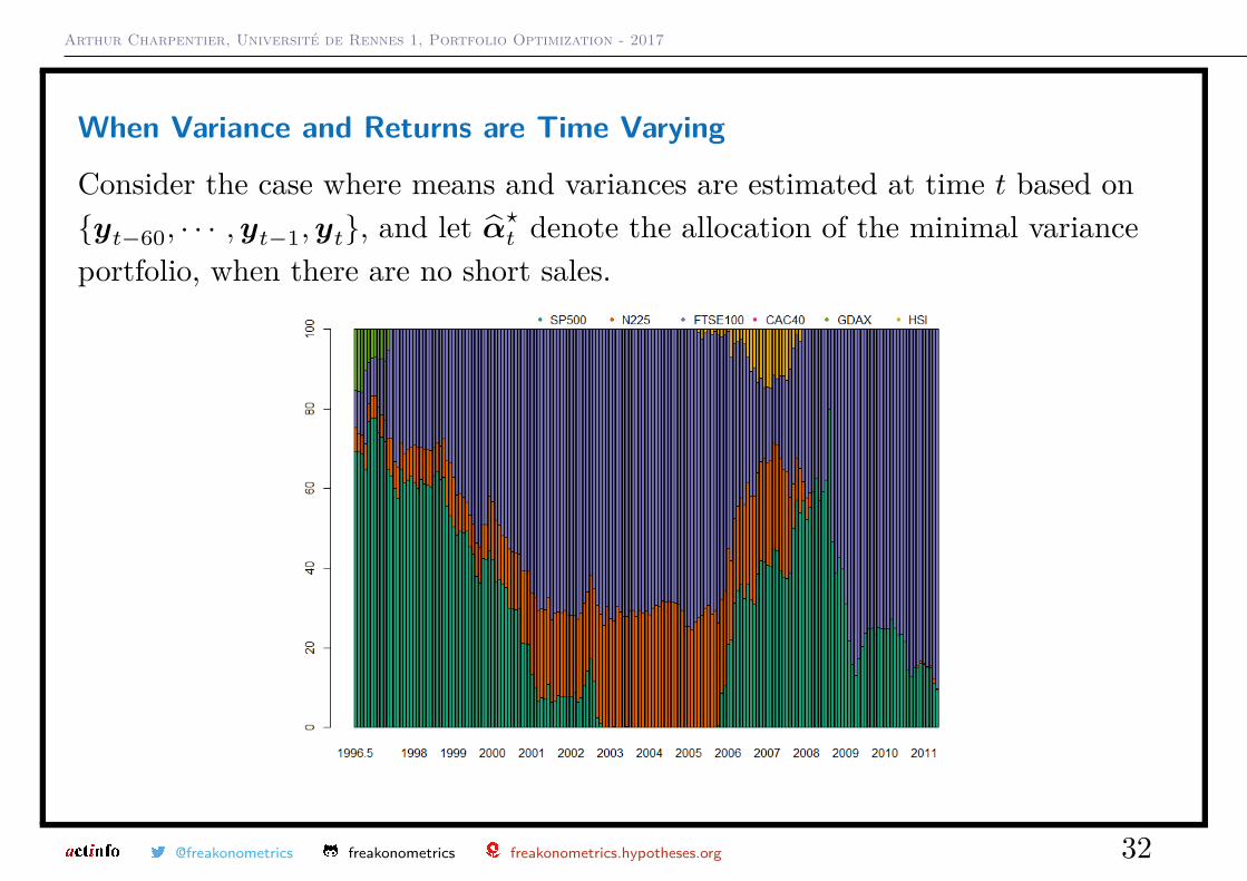
When Variance and Returns are Time Varying
Consider the case where means and variances are estimated at time t based on{yt−60, · · · ,yt−1,yt}, and let α̂?t denote the allocation of the minimal varianceportfolio, when there are no short sales.
@freakonometrics freakonometrics freakonometrics.hypotheses.org 32
Arthur Charpentier, Université de Rennes 1, Portfolio Optimization - 2017
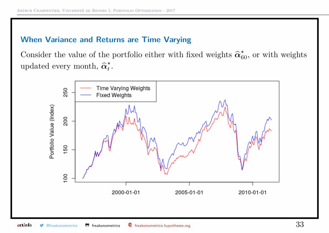
When Variance and Returns are Time Varying
Consider the value of the portfolio either with fixed weights α̂?60, or with weightsupdated every month, α̂?t .
@freakonometrics freakonometrics freakonometrics.hypotheses.org 33
Arthur Charpentier, Université de Rennes 1, Portfolio Optimization - 2017
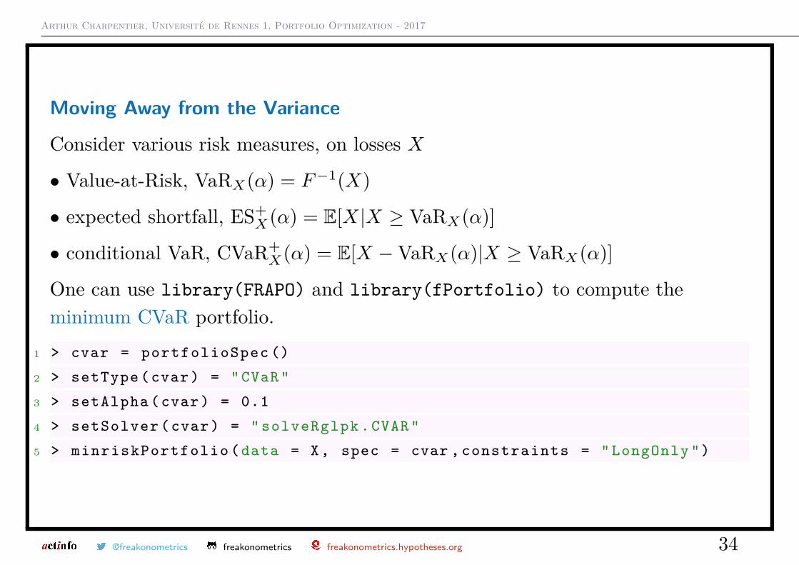
Moving Away from the Variance
Consider various risk measures, on losses X
• Value-at-Risk, VaRX(α) = F−1(X)
• expected shortfall, ES+X(α) = E[X|X ≥ VaRX(α)]
• conditional VaR, CVaR+X(α) = E[X −VaRX(α)|X ≥ VaRX(α)]
One can use library(FRAPO) and library(fPortfolio) to compute theminimum CVaR portfolio.
1 > cvar = portfolioSpec ()
2 > setType (cvar) = "CVaR"
3 > setAlpha (cvar) = 0.1
4 > setSolver (cvar) = " solveRglpk .CVAR"
5 > minriskPortfolio (data = X, spec = cvar , constraints = " LongOnly ")
@freakonometrics freakonometrics freakonometrics.hypotheses.org 34
Arthur Charpentier, Université de Rennes 1, Portfolio Optimization - 2017
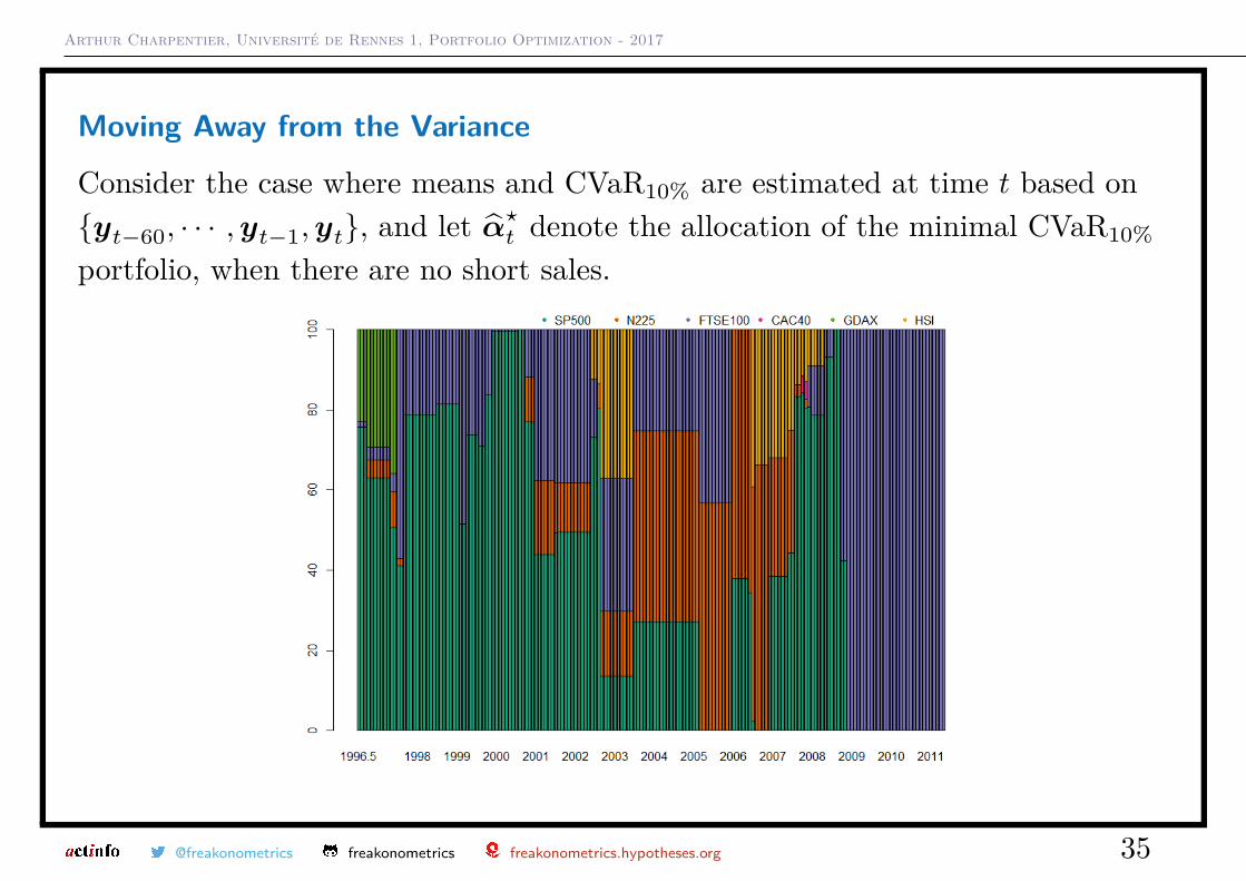
Moving Away from the Variance
Consider the case where means and CVaR10% are estimated at time t based on{yt−60, · · · ,yt−1,yt}, and let α̂?t denote the allocation of the minimal CVaR10%
portfolio, when there are no short sales.
@freakonometrics freakonometrics freakonometrics.hypotheses.org 35
Arthur Charpentier, Université de Rennes 1, Portfolio Optimization - 2017
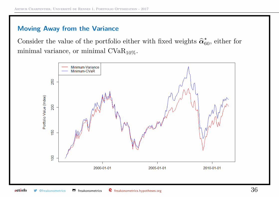
Moving Away from the Variance
Consider the value of the portfolio either with fixed weights α̂?60, either forminimal variance, or minimal CVaR10%.
@freakonometrics freakonometrics freakonometrics.hypotheses.org 36
Arthur Charpentier, Université de Rennes 1, Portfolio Optimization - 2017
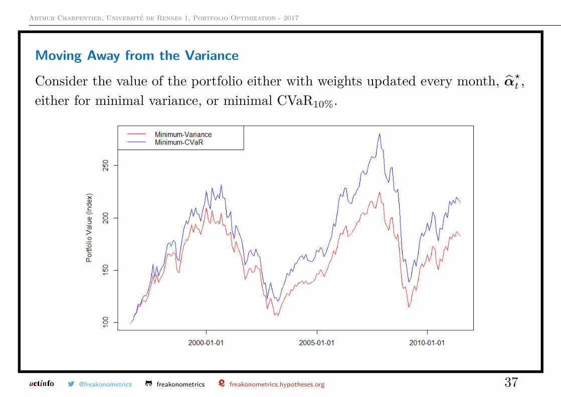
Moving Away from the Variance
Consider the value of the portfolio either with weights updated every month, α̂?t ,either for minimal variance, or minimal CVaR10%.
@freakonometrics freakonometrics freakonometrics.hypotheses.org 37
Arthur Charpentier, Université de Rennes 1, Portfolio Optimization - 2017
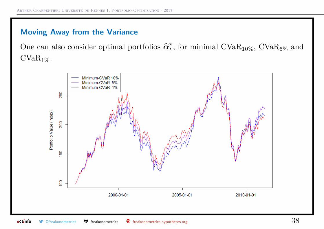
Moving Away from the Variance
One can also consider optimal portfolios α̂?t , for minimal CVaR10%, CVaR5% andCVaR1%.
@freakonometrics freakonometrics freakonometrics.hypotheses.org 38
Recommended