A STUDY OF A SKIRTLESS HOVERCRAFT
DESIGN
THESIS
Edward A. Kelleher, Ensign, USNR
AFIT/GAE/ENY/04-J05
AIR FOR W
APPROVED F
DEPARTMENT OF THE AIR FORCE AIR UNIVERSITY
CE INSTITUTE OF TECHNOLOGY
right-Patterson Air Force Base, Ohio
OR PUBLIC RELEASE; DISTRIBUTION UNLIMITED.

The views expressed in this thesis are those of the author and do not reflect the official policy or position of the United States Navy, United States Air Force, Department of Defense, or the United States Government.
AFIT/GAE/ENY/04-J05
A STUDY OF A SKIRTLESS HOVERCRAFT DESIGN
THESIS
Presented to the Faculty
Department of Aeronautics and Astronautics
Graduate School of Engineering and Management
Air Force Institute of Technology
Air University
Air Education and Training Command
In Partial Fulfillment of the Requirements for the
Degree of Master of Science in Aeronautical Engineering
Edward A. Kelleher, BS
Ensign, USNR
May 2004
APPROVED FOR PUBLIC RELEASE; DISTRIBUTION UNLIMITED.

AFIT/GAE/ENY/04-J05
A STUDY OF A SKIRTLESS HOVERCRAFT DESIGN
Edward A. Kelleher, BS Ensign USNR
Approved: ______ ___________ Dr. Milton Franke (Chairman) date ______ ___________ Lt Col Raymond C. Maple (Member) date ______ ___________ Lt Col Montgomery Houghson (Member) date
Abstract Three proposed skirtless hovercraft designs were analyzed via computational fluid
dynamics to ascertain their lift generation capabilities. The three designs were
adaptations from William Walter’s hybricraft primer and his patent for a fan driven lift
generation device. Each design featured Coanda nozzles, or nozzles that utilize the
Coanda effect, to redirect air flow to aid in the generation of an air curtain around a
central air flow. The designs also utilized a Coanda wing as a lifting body to aid in lift
generation. Each design was set at a height above ground of one foot and a radius of two
feet. The craft was assumed to be axisymmetric around a central axis for a perfectly
circular craft, much like a flying saucer. The craft can be divided into several parts, the
core, the nozzles, the plenum chamber (for designs 2 and 3), and the wing. Flow is
generated from rotor blades situated one foot above the top of the core of the craft. The
nozzles are located at the edges of the craft below the wing. In designs two and three the
plenum chamber is the region between the core and the wing. For each design three
cases were performed where t was increased for each case. This resulted in a total of nine
cases, three cases for three designs. For each case the ratio of nozzle thickness to the
radius of the curved plate, t/R, was set to 0.344 and t was increased while R was
calculated to maintain the ratio. The computational fluid dynamics (CFD) analysis
captured the pressure data and the lift forces were calculated using a pressure differential
analysis. Analysis proved that the hybricraft designs could produce positive lift. While
the first design did not produce positive lift, the second and third designs managed to
generate enough lift to support a craft of a maximum of 52810.24 kg. The max amount
of lift produced was 5388.8 N, while the minimum positive lift generated was 3642.9 N.
iv

Acknowledgments
I would like to thank my thesis advisor, Professor Milton Franke for his help in
this project and his producing of the idea. I would also like to extend my thanks to Lt Col
Maple for all his help with understanding computational fluid dynamics and getting the
computers to work for this thesis. Also, I want to extend a thanks to my fellow ensigns
for their ever diligence in keeping the faith till the end. My final thanks is to my Coach,
Raymond Bautista and the American Fencing Academy of Dayton for giving me
something to distract me when needed.
v
ABSTRACT ................................................................................................................................................ IV LIFT OF FIGURES ................................................................................................................................. VII LIST OF TABLES...................................................................................................................................VIII LIST OF SYMBOLS.................................................................................................................................. IX INTRODUCTION ........................................................................................................................................ 1
BACKGROUND ............................................................................................................................................ 1 BACKGROUND THEORY:............................................................................................................................. 3 CURRENT OBJECTIVES................................................................................................................................ 5
NUMERICAL MODEL SETUP ................................................................................................................. 8 RESULTS.................................................................................................................................................... 14
GENERAL.................................................................................................................................................. 14 DESIGN 1 .................................................................................................................................................. 14 DESIGN 2 .................................................................................................................................................. 19 DESIGN 3 .................................................................................................................................................. 24
ANALYSIS.................................................................................................................................................. 30 GENERAL.................................................................................................................................................. 30 DESIGN 1 .................................................................................................................................................. 31
Case 1: ................................................................................................................................................ 31 Case 2: ................................................................................................................................................ 32 Case 3: ................................................................................................................................................ 33
DESIGN 2 .................................................................................................................................................. 34 Case 1: ................................................................................................................................................ 34 Case 2: ................................................................................................................................................ 35 Case 3: ................................................................................................................................................ 36
DESIGN 3 .................................................................................................................................................. 38 Case 1: ................................................................................................................................................ 38 Case 2: ................................................................................................................................................ 39 Case 3: ................................................................................................................................................ 41
CONCLUSIONS AND RECOMMENDATIONS.................................................................................... 43 APPENDIX A ............................................................................................................................................. 46 APPENDIX B.............................................................................................................................................. 57 SOURCES ................................................................................................................................................... 58 VITAE ......................................................................................................................................................... 59
vi
Lift of Figures Figure 1: Full Scale AVRO Car.......................................................................................... 2 Figure 2: Naudin's Coanda Saucer Epxeriment .................................................................. 4 Figure 3: Schematic of the First Design ............................................................................. 6 Figure 4: Schematic of the Second Design......................................................................... 7 Figure 5: Schematic of the Third Design............................................................................ 8 Figure 6: The Hybrid Grid: A Close Up View of a Nozzle Plate ....................................... 9 Figure 7: The Grid for the First Design, This is a 2-d Planar Cut of the Axisymmetric
Craft .......................................................................................................................... 11 Figure 8: Up Close View of a Coanda Nozzle.................................................................. 12 Figure 9: Pressure (Pa), NASA-2 Spectrum, Design 1 Case 1 ......................................... 14 Figure 10: Velocity Magnitude (m/s), Design 1 Case 1 ................................................... 15 Figure 11: Pressure (Pa), NASA-2 Spectrum, Design 1 Case 2 ....................................... 16 Figure 12: Velocity Magnitude (m/s), Design 1 Case 2 ................................................... 17 Figure 13: Pressure (Pa), NASA-1 Spectrum, Design 1 Case 3 ....................................... 18 Figure 14: Velocity Magnitude (m/s), Design 1 Case 3 ................................................... 19 Figure 15:Pressure (Pa), NASA-1 Spectrum, Design 2, Case 1 ....................................... 20 Figure 16: Velocity Magnitude (m/s), Design 2 Case 1 ................................................... 20 Figure 17: Pressure (Pa), NASA-2 Spectrum, Design 2 Case 2 ....................................... 21 Figure 18: Velocity Magnitude (m/s), Design 2 Case 2 ................................................... 22 Figure 19: Pressure (Pa), NASA-1 Spectrum, Design 2 Case 3 ....................................... 23 Figure 20:Velocity Magnitude (m/s), Design 2 Case 3 .................................................... 24 Figure 21: Pressure (Pa), NASA-1 Spectrum, Design 3 Case 1 ....................................... 25 Figure 22: Velocity Magnitude (m/s), Design 3 Case 1 ................................................... 26 Figure 23: Pressure (Pa), NASA-1 Spectrum, Design 3 Case 2 ....................................... 26 Figure 24: Velocity Magnitude (m/s), Design 3 Case 2 ................................................... 27 Figure 25: Pressure (Pa), NASA-1 Spectrum, Design 3 Case 3 ....................................... 28 Figure 26: Velocity Magnitude (m/s), Design 3 Case 3 ................................................... 29 Figure 27: Pressure Distribution, Design 1 Case 1 ........................................................... 31 Figure 28: Pressure Distribution, Design 1 Case 2 ........................................................... 32 Figure 29: Pressure Distribution, Design 2 Case 2 ........................................................... 36 Figure 30: Pressure Distribution, Design 2 Case 3 ........................................................... 37 Figure 31: Pressure Distribution, Design 3 Case 1 ........................................................... 38 Figure 32: Pressure Distribution, Design 3 Case 2 ........................................................... 40 Figure 33: Pressure Distribution, Design 3 Case 3 ........................................................... 41 Figure 34: Net Force vs. t ................................................................................................. 43
vii

List of Tables Table 1: Domain Sizes in Cells......................................................................................... 10 Table 2: t and R values...................................................................................................... 12 Table 3: Net Forces by Design and Case .......................................................................... 42
viii
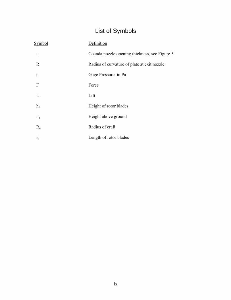
List of Symbols Symbol Definition t Coanda nozzle opening thickness, see Figure 5 R Radius of curvature of plate at exit nozzle p Gage Pressure, in Pa F Force L Lift hb Height of rotor blades hg Height above ground Rc Radius of craft lb Length of rotor blades
ix
Introduction
Background
In 1932 Henri Coanda filed for a French patent on a propulsive device that would
exploit a fluid jet entrainment and attaching phenomena that would later become known
as the Coanda effect. He discovered the phenomena in the early 30’s after it was found to
have caused the destruction of the Coanda-1910, possibly the world’s first jet aircraft.
His experiments using a wind tunnel with smoke and an aerodynamic balance to profile
airfoils led to the discovery of what has become known as the Coanda effect [Green et al.
3].
The Coanda effect is a phenomenon that allows a fluid jet to remain attached to a
wall placed near the fluid jet. This occurs when a free fluid jet exits a nozzle into an
ambient fluid of equal or lower viscosity, which causes entrainment of the ambient fluid.
When a wall is placed near the fluid jet, the fluid jet will attach to the wall. The
entrainment of the ambient fluid becomes partially blocked by the wall, but continues to
be entrained by the jet, thus causing a pressure decrease between the wall and the jet.
This pressure difference causes the jet to move towards the wall. If a low pressure
separation region and vortex form between the wall and jet, the jet will then attach to the
wall [McCarson, 2].
In the 1950’s Avro Canada researched the possibility of a circular wing fighter-
bomber. The initial studies of the craft were abandoned due to lack of funding. In 1954
the United States Air Force and United States Army picked up funding in the hopes of
developing a practical vertical lift craft. In 1959 the VZ-9AV made its first flight.
1

Research at NASA Ames determined the craft to be aerodynamically unstable and the
project was abandoned [Smithsonian, 6].
Figure 1: Full Scale AVRO Car
In September 1998 inventor William Walter received a patent for a lift
augmentation device that utilizes concentric nozzles to provide a central supercharged air
cushion surrounded by an inner central air curtain and an outer or peripheral air cushion
surrounded by a peripheral air curtain. The lift augmentation thus creates a hovercraft
like vehicle that eliminates the skirt in modern hovercraft. This craft differs from
pervious attempts at skirt-less hovercraft in several ways. First, the jet stream producing
source is positioned outside the main body in the form of rotor blades above the main
body. The proposed design also claims to have the ability to navigate obstacles such as
rivers, canyons, and other such natural barriers.
2

Walter’s Hybricaft Primer [Walter, 11] develops the craft in more detail,
explaining the use of Coanda nozzles to generate the air curtains as well as the use of a
Coanda wing, to take advantage of the craft flying within ground effect. The key feature
of these nozzles is the t/R ratio, the thickness of the nozzle to the radius of plate, which is
defined as 0.344 in the 1998 patent. This allows for the air exiting the nozzles to be
deflected back under the craft and thereby creating a sufficient air curtain to support the
craft.
Background Theory: Henri Coanda would later produce multiple patents utilizing the effect he
observed and studied to generate propulsion for aircraft. An experiment by Von Glahn
found that placing curved and flat plates near a nozzle would result in a ratio of lift to
undeflected thrust of about 0.8-0.9, depending on the total deflection angle [Von Glahn,
1]. Thus a Coanda nozzle could achieve a 90˚ deflection of the jet-stream and result in a
vertical lifting force on the order of 0.8 of the undeflected thrust. This shows that Coanda
nozzles can produce lift as well as maintain thrust.
The lift is created on the curved surface of the nozzle where the lower pressure
regions form. Coanda attempted to use this idea with jet engines to generate flow over
outer curved surfaces of crafts he designed. His patent for a lenticular craft give possible
insight to the uses of the Coanda effect in the area of aircraft propulsion [Nijhuis, 8]. The
generation of this lift principle can also be seen in the experimental work of Jean-Louis
Naudin. His Coanda saucer experiment using a simple concave object and high speed
airflow over the top of the object shows that a low pressure region is generated above the
craft. This low pressure region creates lift and causes the craft to hover. The high speed
3
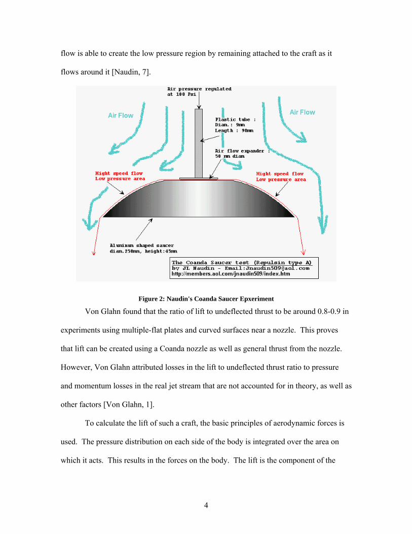
flow is able to create the low pressure region by remaining attached to the craft as it
flows around it [Naudin, 7].
Figure 2: Naudin's Coanda Saucer Epxeriment
Von Glahn found that the ratio of lift to undeflected thrust to be around 0.8-0.9 in
experiments using multiple-flat plates and curved surfaces near a nozzle. This proves
that lift can be created using a Coanda nozzle as well as general thrust from the nozzle.
However, Von Glahn attributed losses in the lift to undeflected thrust ratio to pressure
and momentum losses in the real jet stream that are not accounted for in theory, as well as
other factors [Von Glahn, 1].
To calculate the lift of such a craft, the basic principles of aerodynamic forces is
used. The pressure distribution on each side of the body is integrated over the area on
which it acts. This results in the forces on the body. The lift is the component of the
4
force in the upwards direction [Anderson, 5]. This includes any lift generated by the
rotor blades.
Current Objectives
The scope of this study is to analyze the possibility of a working hybricraft. To
quickly analyze the designs presented a computational analysis was selected to review the
fluid flow around the craft and the validity of the device. Additionally, the thickness of
the Coanda nozzles, t, was varied and analyzed to determine if there is a correlation to the
amount of air needed to flow through the nozzles to generate the correct amount of force
for a proper air curtain and cushion.
Since there were variations in the design of the craft from the patent to the
Hybricraft primer, three designs were developed to be tested. Within each design three
cases were performed to test the variation in t. Fluent® Version 6.1.22 was used to model
and analyze the fluid flow. Each gird was created in the Gridgen® Version 15, grid
generation program. Most post processing was carried out in Fluent®.
Each grid was a mixed grid containing both unstructured and structured cells, also
called a hybrid grid. This was done primarily to pick up any viscous flow around nozzles,
which was necessary to capture the flow features in those regions. A preliminary study
showed that a steady-state flow case would not converge sufficiently and therefore other
options were pursued. The final cases that were utilized in the analysis were performed
as unsteady turbulent cases using a K-epsilon model. Residual convergence is achieved
in the unsteady case on the order of 0.0001. The residual is a measure of how well the
current solution satisfies the discrete form of each governing equation [Bhaskaran, 9].
5
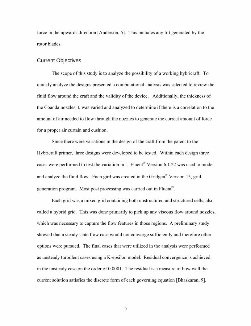
The first design, shown in Figure 3 is based on the drawings taken directly from
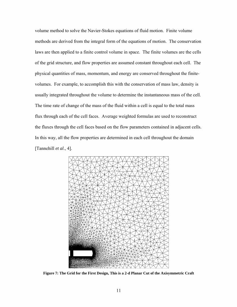
the 1998 patent. Figure 3 shows a 2-D cut plane of the axisymmetric craft, the axis of
symmetry is the X-axis where X=0 is set as the center of the craft. In Figure 3, and all
subsequent designs, the center of the craft is on the far left of the figure. Rotating around
the left edge would generate a symmetrical craft with a four foot diameter. The design
consists of the rotating blades above the craft, common in all designs, and three channels
to direct flow towards the Coanda nozzles.
Figure 3: Schematic of the First Design
The core area also includes a nozzle for air to flow below the craft. The main
feature of this design is the flat nature of it, where the outer surface is not curved up to
the blades, but flat until the outer radius of the craft. The channels that lead to the
nozzles are offset near the rotor blades to allow flow to enter each channel.
6
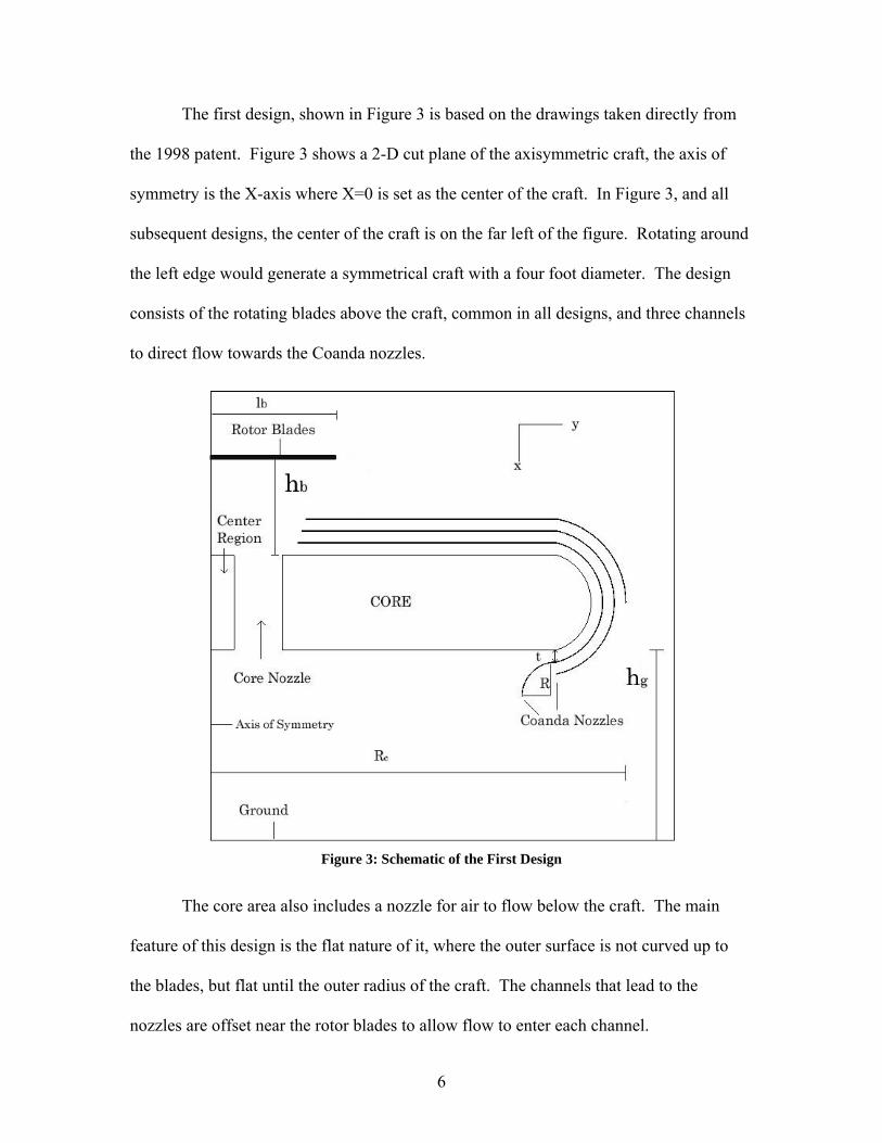
The second design utilizes some similar features of the first design. It, however,
has the outer surface curving up to the blades, thereby forming what Walter refers to as a
Coanda wing, as seen in Figure 4. This surface should allow the air flow to attach to it as
it flows off the edge forming a low pressure region above the craft. This was also seen in
the pressure difference in the experiments performed by Von Glahn [Von Glahn, 1].
Figure 4: Schematic of the Second Design
Additionally this design has the three channels that lead to the Coanda nozzles closely
placed to the intake for the air flow. The core area also includes a channel to direct flow
to the area below the craft.
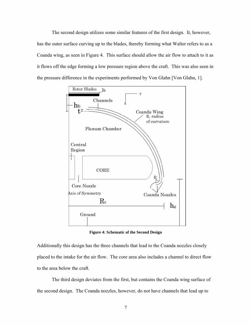
The third design deviates from the first, but contains the Coanda wing surface of
the second design. The Coanda nozzles, however, do not have channels that lead up to
7
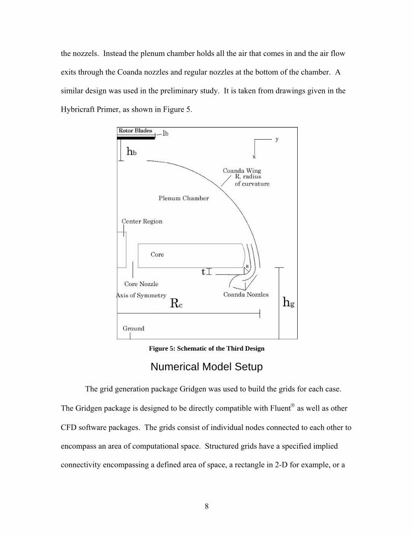
the nozzels. Instead the plenum chamber holds all the air that comes in and the air flow
exits through the Coanda nozzles and regular nozzles at the bottom of the chamber. A
similar design was used in the preliminary study. It is taken from drawings given in the
Hybricraft Primer, as shown in Figure 5.
Figure 5: Schematic of the Third Design
Numerical Model Setup
The grid generation package Gridgen was used to build the grids for each case.
The Gridgen package is designed to be directly compatible with Fluent® as well as other
CFD software packages. The grids consist of individual nodes connected to each other to
encompass an area of computational space. Structured grids have a specified implied
connectivity encompassing a defined area of space, a rectangle in 2-D for example, or a
8
brick in 3-D. In unstructured grids the connectivity must be explicitly specified and
results in triangles in 2-D and tetrahedrons in 3-D. Each cell encompasses an area,
whether it is inside a triangle or rectangle, and can be used in a finite difference scheme
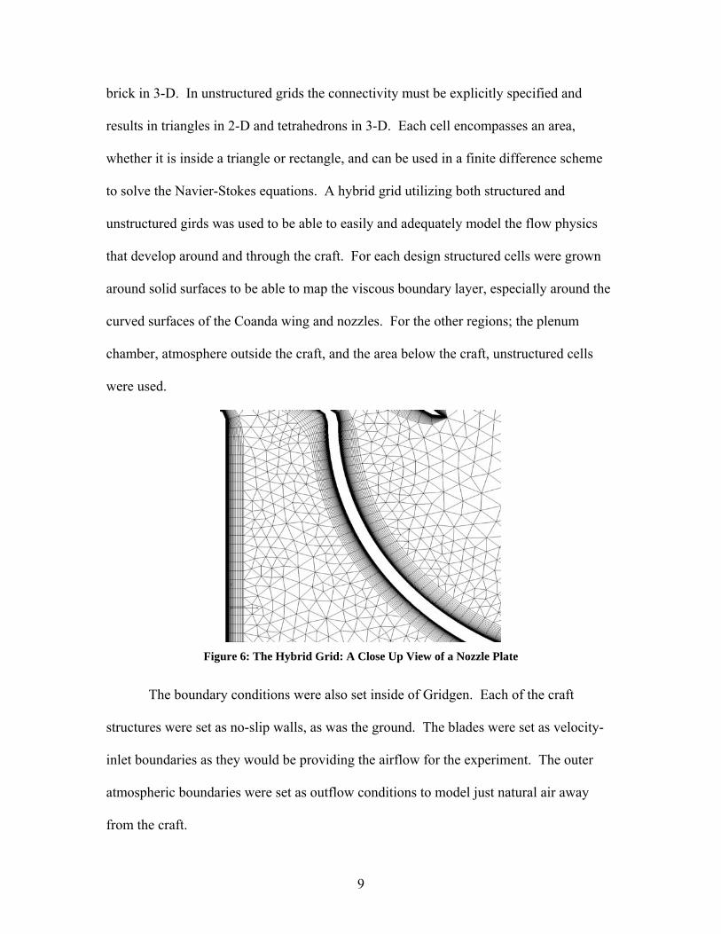
to solve the Navier-Stokes equations. A hybrid grid utilizing both structured and
unstructured girds was used to be able to easily and adequately model the flow physics
that develop around and through the craft. For each design structured cells were grown
around solid surfaces to be able to map the viscous boundary layer, especially around the
curved surfaces of the Coanda wing and nozzles. For the other regions; the plenum
chamber, atmosphere outside the craft, and the area below the craft, unstructured cells
were used.
Figure 6: The Hybrid Grid: A Close Up View of a Nozzle Plate
The boundary conditions were also set inside of Gridgen. Each of the craft
structures were set as no-slip walls, as was the ground. The blades were set as velocity-
inlet boundaries as they would be providing the airflow for the experiment. The outer
atmospheric boundaries were set as outflow conditions to model just natural air away
from the craft.
9
Since the nozzles and core areas are solid areas it was a simple matter of growing
the structured cells from the walls at a specified rate. The initial cell was set to 1E(-6)
with the minimum growth rate of 1E(-4) and a geometric growth rate of 1.1. These were
chosen since they would be small enough to capture the viscous layer and could be grown
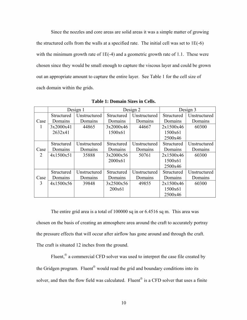
out an appropriate amount to capture the entire layer. See Table 1 for the cell size of
each domain within the grids.
Table 1: Domain Sizes in Cells.
Design 1 Design 2 Design 3 Structured Domains
Unstructured Domains
Structured Domains
Unstructured Domains
Structured Domains
Unstructured Domains
Case
1 3x2000x41 2632x41
44865 3x2000x461500x61
44667 2x1500x46 1500x61 2500x46
60300
Structured Domains
Unstructured Domains
Structured Domains
Unstructured Domains
Structured Domains
Unstructured Domains
Case
2 4x1500x51 35888 3x2000x562000x61
50761 2x1500x46 1500x61 2500x46
60300
Structured Domains
Unstructured Domains
Structured Domains
Unstructured Domains
Structured Domains
Unstructured Domains
Case
3 4x1500x56 39848 3x2500x56200x61
49855 2x1500x46 1500x61 2500x46
60300
The entire grid area is a total of 100000 sq in or 6.4516 sq m. This area was
chosen on the basis of creating an atmosphere area around the craft to accurately portray
the pressure effects that will occur after airflow has gone around and through the craft.
The craft is situated 12 inches from the ground.
Fluent,® a commercial CFD solver was used to interpret the case file created by
the Gridgen program. Fluent® would read the grid and boundary conditions into its
solver, and then the flow field was calculated. Fluent® is a CFD solver that uses a finite
10
volume method to solve the Navier-Stokes equations of fluid motion. Finite volume
methods are derived from the integral form of the equations of motion. The conservation
laws are then applied to a finite control volume in space. The finite volumes are the cells
of the grid structure, and flow properties are assumed constant throughout each cell. The
physical quantities of mass, momentum, and energy are conserved throughout the finite-
volumes. For example, to accomplish this with the conservation of mass law, density is
usually integrated throughout the volume to determine the instantaneous mass of the cell.
The time rate of change of the mass of the fluid within a cell is equal to the total mass
flux through each of the cell faces. Average weighted formulas are used to reconstruct
the fluxes through the cell faces based on the flow parameters contained in adjacent cells.
In this way, all the flow properties are determined in each cell throughout the domain
[Tannehill et al., 4].
Figure 7: The Grid for the First Design, This is a 2-d Planar Cut of the Axisymmetric Craft
11
Within Fluent® the velocity conditions on the rotor blades were set to be 100 m/s.
This was chosen based on a preliminary study performed on a similar craft (Appendix A)
which looked at speeds of 25, 50, and 100 m/s. In these cases only the 100 m/s flow
caused the flow to remain attached to the surface. Additionally the atmospheric pressure
was set to 101325 Pa, so the returned pressure data would be in gage pressure.
Fluent® has both steady and unsteady flow solvers. In the preliminary study of
appendix A, it was found that the steady solvers did not sufficiently converge to the
desired values. However, an unsteady trial proved to drive the residuals to an acceptable
convergence level. From there a time step was chosen to time accurately model the flow
field. This causes Fluent® to set the global time step used with each cell to be calculated.
Local sub-iterations are performed for each time step. The time step chosen was 0.001 s
with 20 iterations per time step. Each case was initially run for 1000 time steps, or a full
1 second.
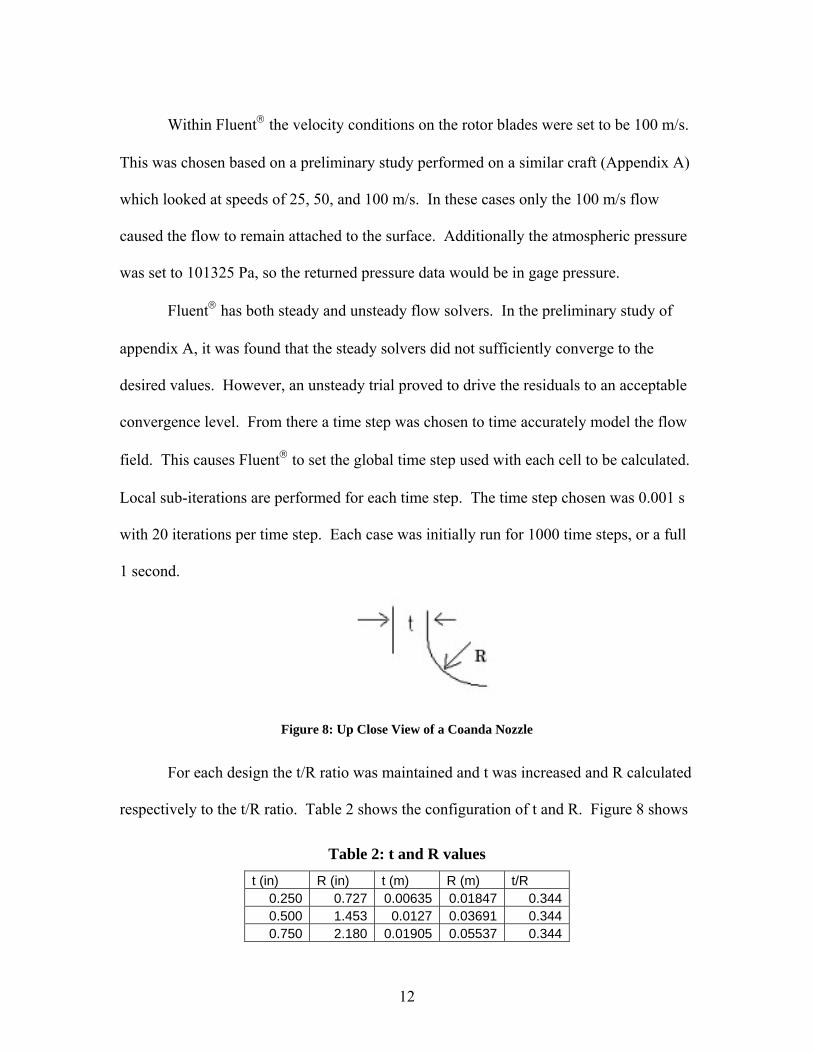
Figure 8: Up Close View of a Coanda Nozzle
For each design the t/R ratio was maintained and t was increased and R calculated
respectively to the t/R ratio. Table 2 shows the configuration of t and R. Figure 8 shows
Table 2: t and R values t (in) R (in) t (m) R (m) t/R
0.250 0.727 0.00635 0.01847 0.3440.500 1.453 0.0127 0.03691 0.3440.750 2.180 0.01905 0.05537 0.344
12
t and R in physical reference to the nozzles. The effects of expanding t were then
recorded in the form of pressure data from Fluent®. To analyze the results both Fluent®
and FieldView®; Version 9, a flow visualization package designed for post-processing,
were used to visualize and determine the flow characteristics. From the pressure and
velocity data the lift can be determined from pressure differentials around the craft.
For each case Rc was set to 0.6096 m, hg was set to 0.3048 m, and lb was set to
0.3048 m. For designs two and three the total height of the craft was set to 0.3048 m and
for design one the total height was 0.1524 m. For design one, hb was set to 0.3048 m
above the top surface of the core, for design two hb was 0.3048 m from the lowest
channel surface, and for design three hb was 0.3048 m from the Coanda wing surface.
The overlap region of the rotor blades over the first surface was a maximum of 0.1524 m.
13

Results
General The results show in most cases that a high pressure region generally forms below
the core nozzle. This region is relatively small and bares little to no effect on the craft.
The region at a distance Rc from the center axis of the craft also develops some higher
pressures in cases where t is larger than 0.0127. For designs two and three it can be seen
that some vortices appear, both inside the plenum chamber and below the craft. The high
pressure regions directly below the rotor blades and above the center region appear in all
cases and designs.
Design 1 Figure 9 shows the pressure data for the first case of this design. The figure
shows that while the high pressure region does form below the core nozzle, the rest of the
region below the craft actually drops in pressure. The region below the center region
maintains a higher pressure due to the constant flow from the rotor blades through the
core nozzle.
Figure 9: Pressure (Pa), NASA-2 Spectrum, Design 1 Case 1
14
The flow through the channels to the nozzles remains at a relatively constant
pressure until reaching the nozzles where there is a slight pressure drop. The region
below the craft loses most of its flow to the ambient air because no air curtain is formed
to force the flow back into the region below the craft, and the flow maintains a velocity
outwards into the ambient air. The flow across the top of the craft has a velocity fast
enough to lower the pressure in that region. From Figure 9 it would seem that the
pressures above and below the craft would result in almost no lift. The high pressure
regions on the center region and the region directly under the rotor blades would create
negative lift forces.
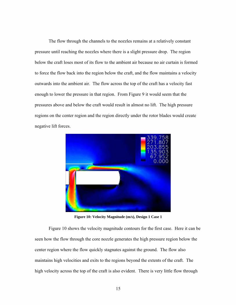
Figure 10: Velocity Magnitude (m/s), Design 1 Case 1
Figure 10 shows the velocity magnitude contours for the first case. Here it can be
seen how the flow through the core nozzle generates the high pressure region below the
center region where the flow quickly stagnates against the ground. The flow also
maintains high velocities and exits to the regions beyond the extents of the craft. The
high velocity across the top of the craft is also evident. There is very little flow through
15
the Coanda nozzles and therefore they have little effect to maintain any pressure region
below the craft.
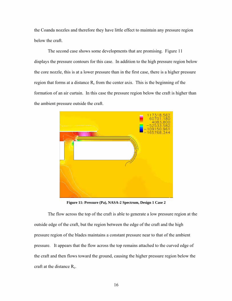
The second case shows some developments that are promising. Figure 11
displays the pressure contours for this case. In addition to the high pressure region below
the core nozzle, this is at a lower pressure than in the first case, there is a higher pressure
region that forms at a distance Rc from the center axis. This is the beginning of the
formation of an air curtain. In this case the pressure region below the craft is higher than
the ambient pressure outside the craft.
Figure 11: Pressure (Pa), NASA-2 Spectrum, Design 1 Case 2
The flow across the top of the craft is able to generate a low pressure region at the
outside edge of the craft, but the region between the edge of the craft and the high
pressure region of the blades maintains a constant pressure near to that of the ambient
pressure. It appears that the flow across the top remains attached to the curved edge of
the craft and then flows toward the ground, causing the higher pressure region below the
craft at the distance Rc.
16
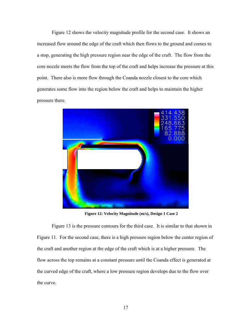
Figure 12 shows the velocity magnitude profile for the second case. It shows an
increased flow around the edge of the craft which then flows to the ground and comes to
a stop, generating the high pressure region near the edge of the craft. The flow from the
core nozzle meets the flow from the top of the craft and helps increase the pressure at this
point. There also is more flow through the Coanda nozzle closest to the core which
generates some flow into the region below the craft and helps to maintain the higher
pressure there.
Figure 12: Velocity Magnitude (m/s), Design 1 Case 2
Figure 13 is the pressure contours for the third case. It is similar to that shown in
Figure 11. For the second case, there is a high pressure region below the center region of
the craft and another region at the edge of the craft which is at a higher pressure. The
flow across the top remains at a constant pressure until the Coanda effect is generated at
the curved edge of the craft, where a low pressure region develops due to the flow over
the curve.
17
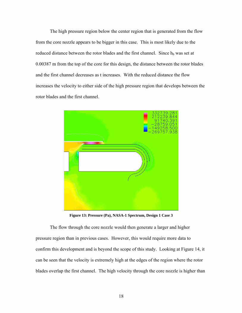
The high pressure region below the center region that is generated from the flow
from the core nozzle appears to be bigger in this case. This is most likely due to the
reduced distance between the rotor blades and the first channel. Since hb was set at
0.00387 m from the top of the core for this design, the distance between the rotor blades
and the first channel decreases as t increases. With the reduced distance the flow
increases the velocity to either side of the high pressure region that develops between the
rotor blades and the first channel.
Figure 13: Pressure (Pa), NASA-1 Spectrum, Design 1 Case 3
The flow through the core nozzle would then generate a larger and higher
pressure region than in previous cases. However, this would require more data to
confirm this development and is beyond the scope of this study. Looking at Figure 14, it
can be seen that the velocity is extremely high at the edges of the region where the rotor
blades overlap the first channel. The high velocity through the core nozzle is higher than
18

previous cases and, therefore, would indeed create a higher pressure region when it
stagnates near the ground.
Figure 14: Velocity Magnitude (m/s), Design 1 Case 3
Design 2 This design proved to have interesting results that could generate positive lift
forces on the craft. Figure 15 shows the pressure for the first case of this design. The
region below the craft has developed two high pressure regions: one below the center
region and one below the Coanda nozzle and Coanda wing surface. Flow through the
core nozzle serves to maintain the high pressure below the center region. This also serves
to maintain a pressure cushion below the craft. This pressure cushion is also maintained
by the higher pressure region below the Coanda wing surface at a distance Rc from the
center axis which serves as an air curtain, creating a pressure wall and keeping the higher
pressure flow beneath the core of the craft.
19
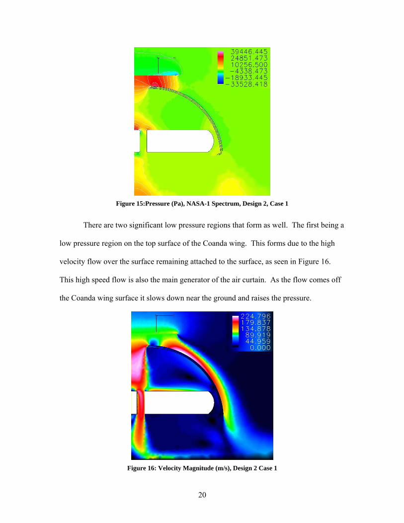
Figure 15:Pressure (Pa), NASA-1 Spectrum, Design 2, Case 1
There are two significant low pressure regions that form as well. The first being a
low pressure region on the top surface of the Coanda wing. This forms due to the high
velocity flow over the surface remaining attached to the surface, as seen in Figure 16.
This high speed flow is also the main generator of the air curtain. As the flow comes off
the Coanda wing surface it slows down near the ground and raises the pressure.
Figure 16: Velocity Magnitude (m/s), Design 2 Case 1
20
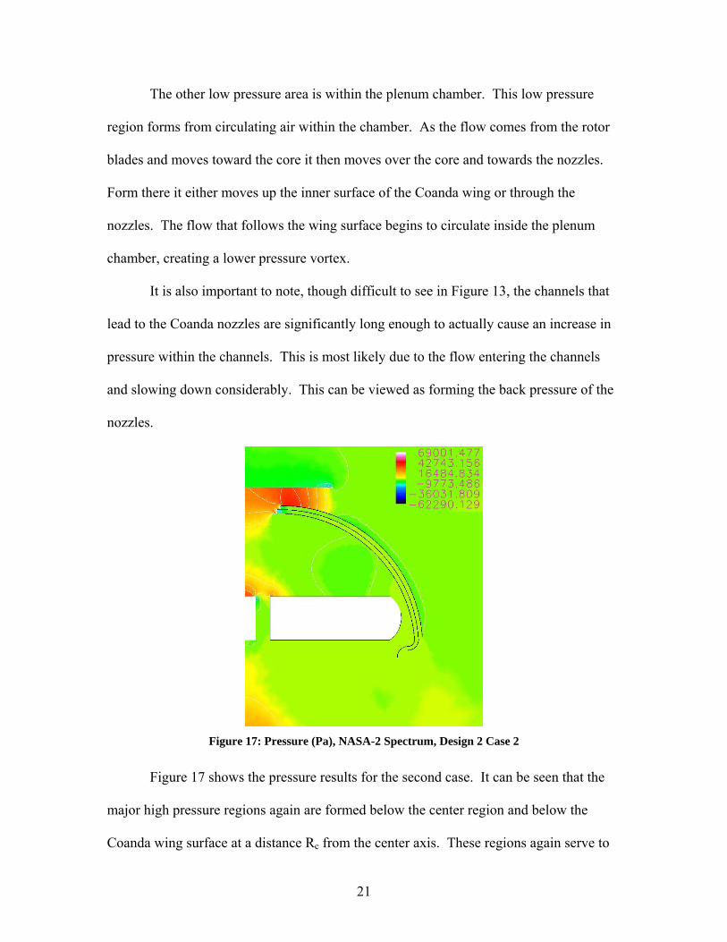
The other low pressure area is within the plenum chamber. This low pressure
region forms from circulating air within the chamber. As the flow comes from the rotor
blades and moves toward the core it then moves over the core and towards the nozzles.
Form there it either moves up the inner surface of the Coanda wing or through the
nozzles. The flow that follows the wing surface begins to circulate inside the plenum
chamber, creating a lower pressure vortex.
It is also important to note, though difficult to see in Figure 13, the channels that
lead to the Coanda nozzles are significantly long enough to actually cause an increase in
pressure within the channels. This is most likely due to the flow entering the channels
and slowing down considerably. This can be viewed as forming the back pressure of the
nozzles.
Figure 17: Pressure (Pa), NASA-2 Spectrum, Design 2 Case 2
Figure 17 shows the pressure results for the second case. It can be seen that the
major high pressure regions again are formed below the center region and below the
Coanda wing surface at a distance Rc from the center axis. These regions again serve to
21
maintain the pressure cushion below the craft, which is at a pressure higher than the
ambient pressure around the craft. It should be noted that the air curtain in this case
appears to be smaller and of lower pressure than the previous case.
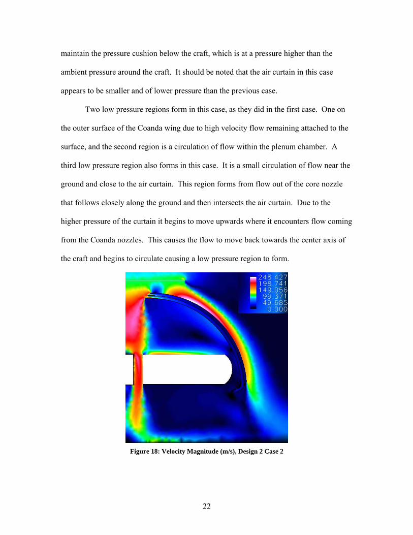
Two low pressure regions form in this case, as they did in the first case. One on
the outer surface of the Coanda wing due to high velocity flow remaining attached to the
surface, and the second region is a circulation of flow within the plenum chamber. A
third low pressure region also forms in this case. It is a small circulation of flow near the
ground and close to the air curtain. This region forms from flow out of the core nozzle
that follows closely along the ground and then intersects the air curtain. Due to the
higher pressure of the curtain it begins to move upwards where it encounters flow coming
from the Coanda nozzles. This causes the flow to move back towards the center axis of
the craft and begins to circulate causing a low pressure region to form.
Figure 18: Velocity Magnitude (m/s), Design 2 Case 2
22
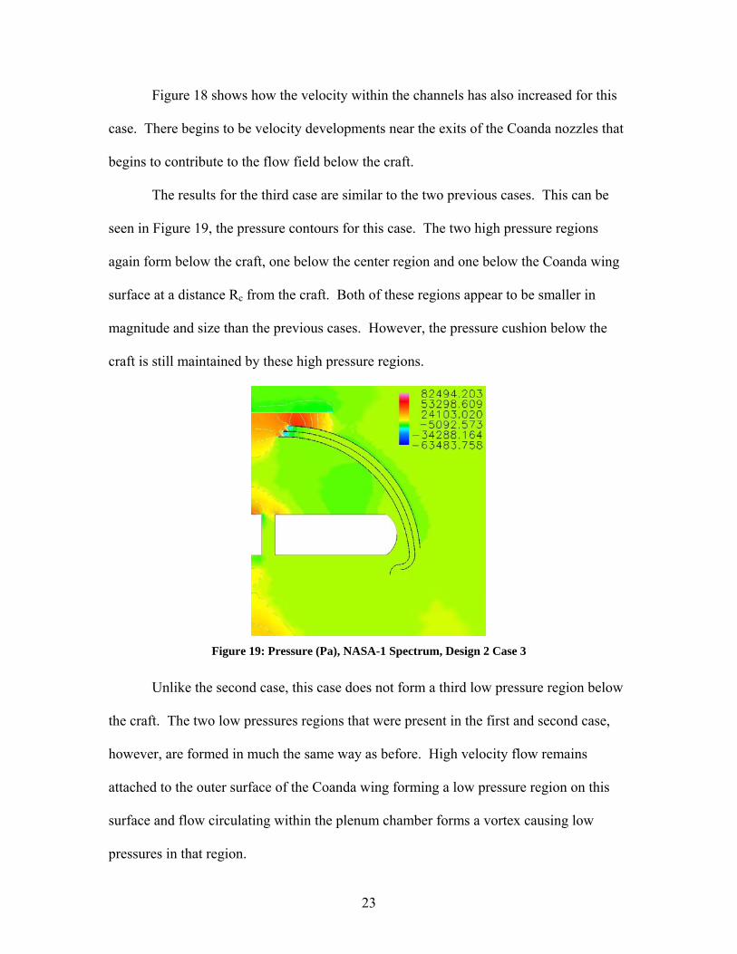
Figure 18 shows how the velocity within the channels has also increased for this
case. There begins to be velocity developments near the exits of the Coanda nozzles that
begins to contribute to the flow field below the craft.
The results for the third case are similar to the two previous cases. This can be
seen in Figure 19, the pressure contours for this case. The two high pressure regions
again form below the craft, one below the center region and one below the Coanda wing
surface at a distance Rc from the craft. Both of these regions appear to be smaller in
magnitude and size than the previous cases. However, the pressure cushion below the
craft is still maintained by these high pressure regions.
Figure 19: Pressure (Pa), NASA-1 Spectrum, Design 2 Case 3
Unlike the second case, this case does not form a third low pressure region below
the craft. The two low pressures regions that were present in the first and second case,
however, are formed in much the same way as before. High velocity flow remains
attached to the outer surface of the Coanda wing forming a low pressure region on this
surface and flow circulating within the plenum chamber forms a vortex causing low
pressures in that region.
23
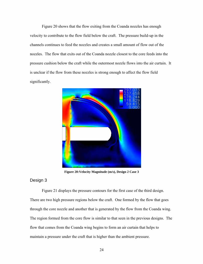
Figure 20 shows that the flow exiting from the Coanda nozzles has enough
velocity to contribute to the flow field below the craft. The pressure build-up in the
channels continues to feed the nozzles and creates a small amount of flow out of the
nozzles. The flow that exits out of the Coanda nozzle closest to the core feeds into the
pressure cushion below the craft while the outermost nozzle flows into the air curtain. It
is unclear if the flow from these nozzles is strong enough to affect the flow field
significantly.
Figure 20:Velocity Magnitude (m/s), Design 2 Case 3
Design 3 Figure 21 displays the pressure contours for the first case of the third design.
There are two high pressure regions below the craft. One formed by the flow that goes
through the core nozzle and another that is generated by the flow from the Coanda wing.
The region formed from the core flow is similar to that seen in the previous designs. The
flow that comes from the Coanda wing begins to form an air curtain that helps to
maintain a pressure under the craft that is higher than the ambient pressure.
24
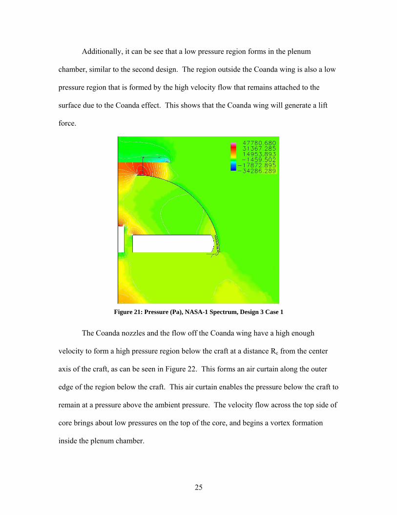
Additionally, it can be see that a low pressure region forms in the plenum
chamber, similar to the second design. The region outside the Coanda wing is also a low
pressure region that is formed by the high velocity flow that remains attached to the
surface due to the Coanda effect. This shows that the Coanda wing will generate a lift
force.
Figure 21: Pressure (Pa), NASA-1 Spectrum, Design 3 Case 1
The Coanda nozzles and the flow off the Coanda wing have a high enough
velocity to form a high pressure region below the craft at a distance Rc from the center
axis of the craft, as can be seen in Figure 22. This forms an air curtain along the outer
edge of the region below the craft. This air curtain enables the pressure below the craft to
remain at a pressure above the ambient pressure. The velocity flow across the top side of
core brings about low pressures on the top of the core, and begins a vortex formation
inside the plenum chamber.
25

Figure 22: Velocity Magnitude (m/s), Design 3 Case 1
Figure 23 shows a very similar pressure profile for the second case. However, the
high pressure region below the center region appears to dissipate faster, most likely due
to slightly lower velocities passing though the core nozzle. This can be seen by
comparing Figure 22 to Figure 24.
Figure 23: Pressure (Pa), NASA-1 Spectrum, Design 3 Case 2
26
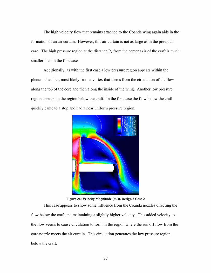
The high velocity flow that remains attached to the Coanda wing again aids in the
formation of an air curtain. However, this air curtain is not as large as in the previous
case. The high pressure region at the distance Rc from the center axis of the craft is much
smaller than in the first case.
Additionally, as with the first case a low pressure region appears within the
plenum chamber, most likely from a vortex that forms from the circulation of the flow
along the top of the core and then along the inside of the wing. Another low pressure
region appears in the region below the craft. In the first case the flow below the craft
quickly came to a stop and had a near uniform pressure region.
Figure 24: Velocity Magnitude (m/s), Design 3 Case 2
This case appears to show some influence from the Coanda nozzles directing the
flow below the craft and maintaining a slightly higher velocity. This added velocity to
the flow seems to cause circulation to form in the region where the run off flow from the
core nozzle meets the air curtain. This circulation generates the low pressure region
below the craft.
27
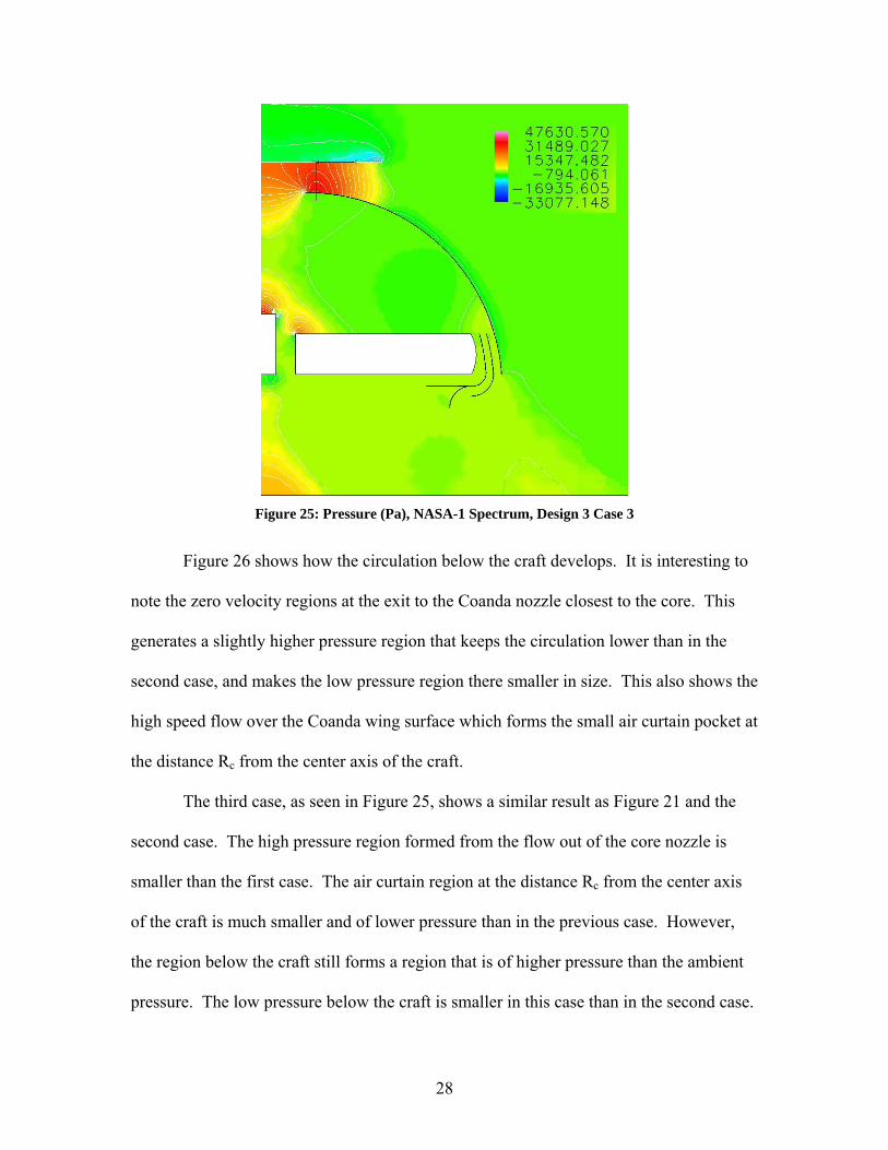
Figure 25: Pressure (Pa), NASA-1 Spectrum, Design 3 Case 3
Figure 26 shows how the circulation below the craft develops. It is interesting to
note the zero velocity regions at the exit to the Coanda nozzle closest to the core. This
generates a slightly higher pressure region that keeps the circulation lower than in the
second case, and makes the low pressure region there smaller in size. This also shows the
high speed flow over the Coanda wing surface which forms the small air curtain pocket at
the distance Rc from the center axis of the craft.
The third case, as seen in Figure 25, shows a similar result as Figure 21 and the
second case. The high pressure region formed from the flow out of the core nozzle is
smaller than the first case. The air curtain region at the distance Rc from the center axis
of the craft is much smaller and of lower pressure than in the previous case. However,
the region below the craft still forms a region that is of higher pressure than the ambient
pressure. The low pressure below the craft is smaller in this case than in the second case.
28

The low pressure region within the plenum chamber, however, seems to be larger than
the previous case. This larger low pressure region within the plenum chamber may affect
the lift generation of the Coanda wing.
Figure 26: Velocity Magnitude (m/s), Design 3 Case 3
29
Analysis
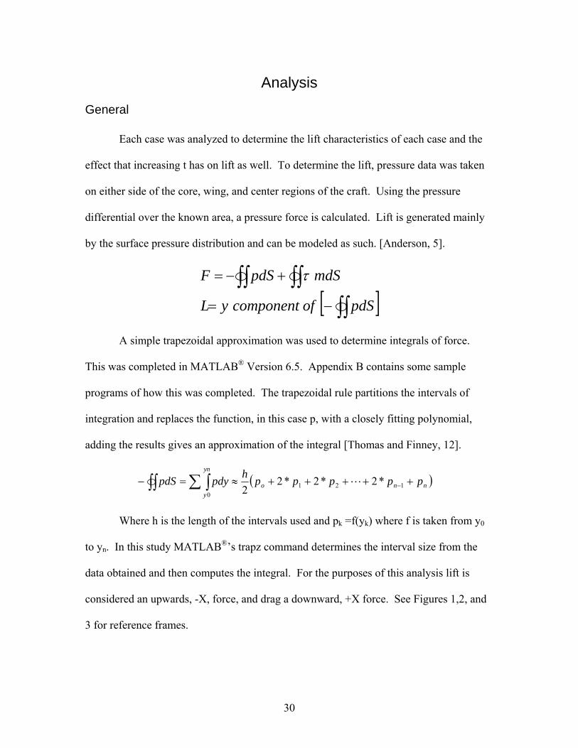
General Each case was analyzed to determine the lift characteristics of each case and the
effect that increasing t has on lift as well. To determine the lift, pressure data was taken
on either side of the core, wing, and center regions of the craft. Using the pressure
differential over the known area, a pressure force is calculated. Lift is generated mainly
by the surface pressure distribution and can be modeled as such. [Anderson, 5].
[ ]∫∫∫∫ ∫∫
−=
+−=
pdSofcomponentyL
mdSpdSF τ
A simple trapezoidal approximation was used to determine integrals of force.
This was completed in MATLAB® Version 6.5. Appendix B contains some sample
programs of how this was completed. The trapezoidal rule partitions the intervals of
integration and replaces the function, in this case p, with a closely fitting polynomial,
adding the results gives an approximation of the integral [Thomas and Finney, 12].
( )∫∫ ∑ ∫ +++++≈=− − nno
yn
y
ppppphpdypdS 1210
*2*2*22
L
Where h is the length of the intervals used and pk =f(yk) where f is taken from y0
to yn. In this study MATLAB®’s trapz command determines the interval size from the
data obtained and then computes the integral. For the purposes of this analysis lift is
considered an upwards, -X, force, and drag a downward, +X force. See Figures 1,2, and
3 for reference frames.
30
Design 1
Case 1:
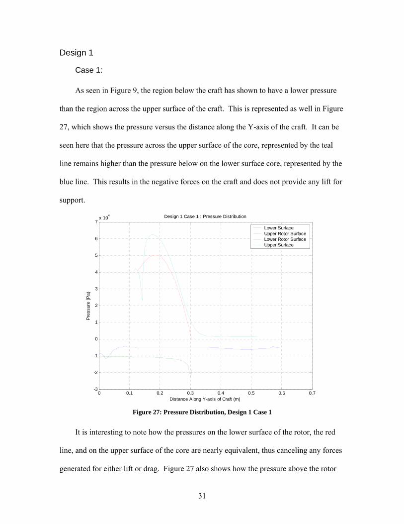
As seen in Figure 9, the region below the craft has shown to have a lower pressure
than the region across the upper surface of the craft. This is represented as well in Figure
27, which shows the pressure versus the distance along the Y-axis of the craft. It can be
seen here that the pressure across the upper surface of the core, represented by the teal
line remains higher than the pressure below on the lower surface core, represented by the
blue line. This results in the negative forces on the craft and does not provide any lift for
support.
0 0.1 0.2 0.3 0.4 0.5 0.6 0.7-3
-2
-1
0
1
2
3
4
5
6
7x 10⁴ Design 1 Case 1 : Pressure Distribution
Distance Along Y-axis of Craft (m)
Pre
ssur
e (P
a)
Lower SurfaceUpper Rotor SurfaceLower Rotor SurfaceUpper Surface
Figure 27: Pressure Distribution, Design 1 Case 1
It is interesting to note how the pressures on the lower surface of the rotor, the red
line, and on the upper surface of the core are nearly equivalent, thus canceling any forces
generated for either lift or drag. Figure 27 also shows how the pressure above the rotor
31
blades are very low, represented by the green line, and could possibly allow for lift
generation if the pressures below the rotor are large enough.
The pressure differential analysis for this case proved that this design would not
work and actually generates negative lift. The total force for this design was -48.0628 N.
This net negative force is the result of extreme pressure differentials between the pressure
on the upper surface of the craft and the pressure on the lower surface of the craft.
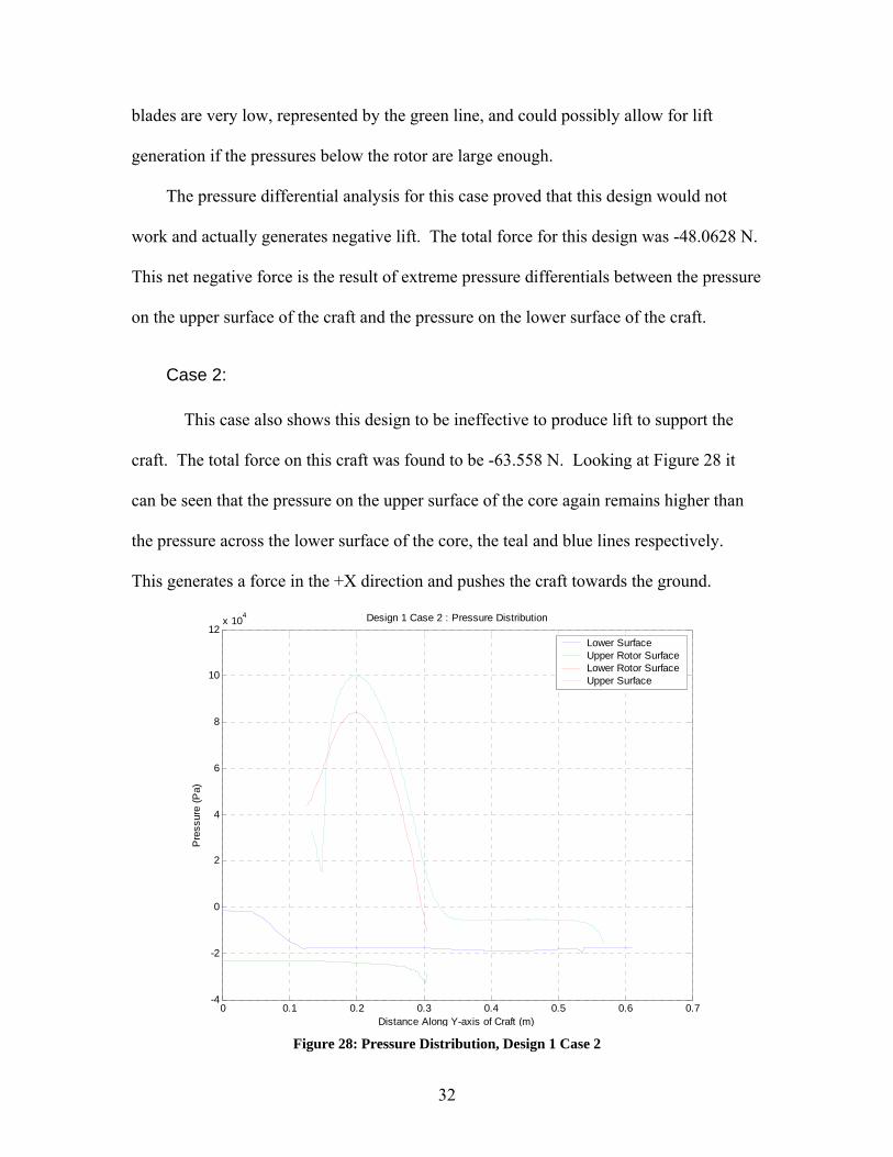
Case 2:
This case also shows this design to be ineffective to produce lift to support the
craft. The total force on this craft was found to be -63.558 N. Looking at Figure 28 it
can be seen that the pressure on the upper surface of the core again remains higher than
the pressure across the lower surface of the core, the teal and blue lines respectively.
This generates a force in the +X direction and pushes the craft towards the ground.
0 0.1 0.2 0.3 0.4 0.5 0.6 0.7-4
-2
0
2
4
6
8
10
12x 104 Design 1 Case 2 : Pressure Distribution
Distance Along Y-axis of Craft (m)
Pre
ssur
e (P
a)
Lower SurfaceUpper Rotor SurfaceLower Rotor SurfaceUpper Surface
Figure 28: Pressure Distribution, Design 1 Case 2
32

Again the pressures in the region below the rotor are of similar magnitudes.
There is an increase in the maximum magnitude of the pressure on the lower surface of
the rotor blades. There is also an increase in the magnitude of the pressure on the lower
surface of the craft near the axis. Additionally, the pressures above the rotor blades have
decreased in magnitude. However, these facets prove not to contribute any additional lift
forces.
Case 3:
Continuing the trend of the first two cases, this case shows that the design
produces negative lift. This case proves to have the highest amount of negative lift
producing a total of -109.376 N. Figure 29, shows the pressure distribution across for
this case.
0 0.1 0.2 0.3 0.4 0.5 0.6 0.7-1
-0.5
0
0.5
1
1.5
2
2.5
3
3.5x 10
5 Design 1 Case 3 : Pressure Distribution
Distance Along Y-axis of Craft (m)
Pre
ssur
e (P
a)
Lower SurfaceUpper Rotor SurfaceLower Rotor SurfaceUpper Surface
Figure 29: Pressure Distribution, Design 1 Case 3
33

While the pressures in the overlap region are almost equal, the red and teal lines,
the pressure above the rotor blades has also increased, seen in the green line. The
pressures along the lower surface of the craft continue to remain at similar levels as the
first two cases for this design. This trend and the growth of the pressure above the rotor
blades contribute to the loss of lift for this case.
Design 2
Case 1:
This is the first case to produce positive lift on the craft. Overall, this case
generated 3642.9 N of lift. Figure 30 depicts the pressure distribution across the craft. It
can be seen that the pressure along the upper surface, teal, actually drops below the
pressure on the lower surface, blue, of the craft. This creates a significant amount of lift.
0 0.1 0.2 0.3 0.4 0.5 0.6 0.7-2
-1
0
1
2
3
4x 10
4 Design 2 Case 1 : Pressure Distribution
Distance Along Y-axis of Craft (m)
Pre
ssur
e (P
a)
Lower SurfaceUpper Rotor SurfaceLower Rotor SurfaceUpper Wing SurfaceOverlap Region
Figure 30: Pressure Distribution, Design 2 Case 1
34
The pressure drop along the upper surface is due to the flow attachment to the
Coanda wing surface. This attachment allows the flow to remain at high speeds and
lower the pressure on this outer surface. The pressures are low enough to allow the
pressure cushion to generate forces to support a craft of 35,700 kg.
The pressure acting on the wing surface in the overlap region, shown in purple, is
nearly equivalent to the pressure on the lower surface of the rotor blades, depicted in red.
This trend continues from the first design and shows the little effect of the pressures in
this region on generating force. This case lacks data for the lower surface, blue, in the
region beyond the overlap area. It is possible that more lift could have been produced
due to the low magnitudes of the pressure above the rotor blades. However, these
pressures are not lower than those in the first design.
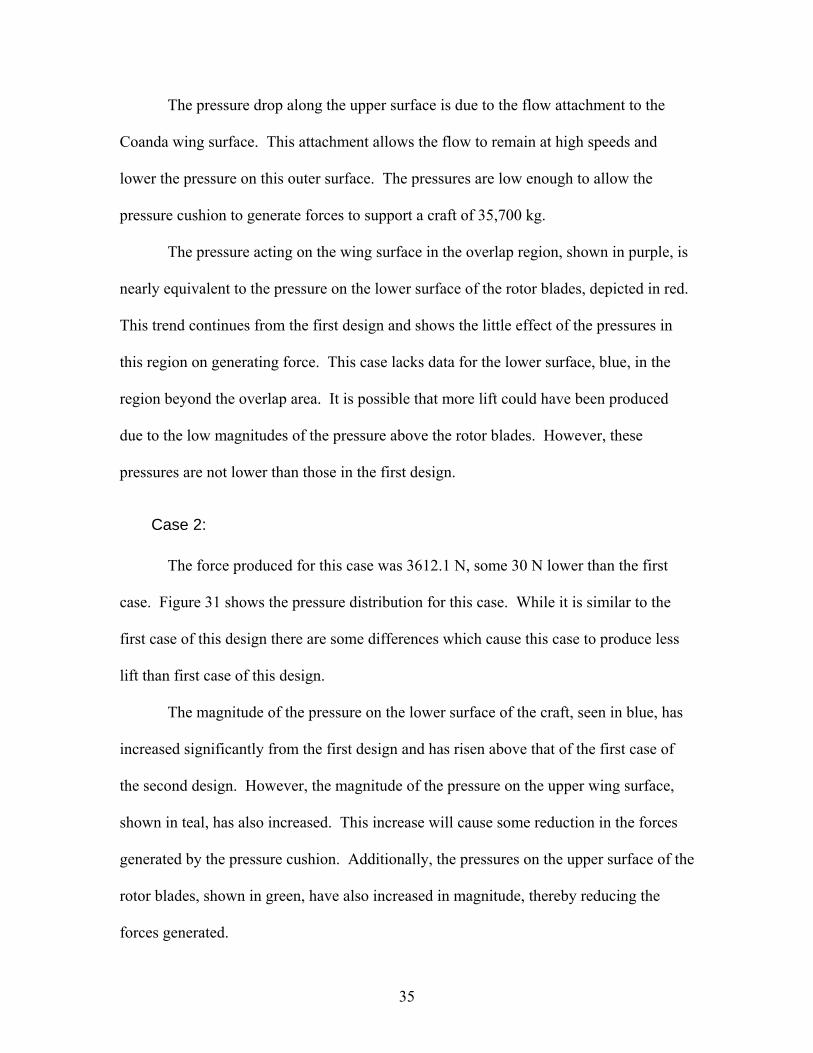
Case 2:
The force produced for this case was 3612.1 N, some 30 N lower than the first
case. Figure 31 shows the pressure distribution for this case. While it is similar to the
first case of this design there are some differences which cause this case to produce less
lift than first case of this design.
The magnitude of the pressure on the lower surface of the craft, seen in blue, has
increased significantly from the first design and has risen above that of the first case of
the second design. However, the magnitude of the pressure on the upper wing surface,
shown in teal, has also increased. This increase will cause some reduction in the forces
generated by the pressure cushion. Additionally, the pressures on the upper surface of the
rotor blades, shown in green, have also increased in magnitude, thereby reducing the
forces generated.
35
0 0.1 0.2 0.3 0.4 0.5 0.6 0.7-2
-1
0
1
2
3
4x 10
4 Design 2 Case 2 : Pressure Distribution
Distance Along Y-axis of Craft (m)
Pre
ssur
e (P
a)
Lower SurfaceUpper Rotor SurfaceLower Rotor SurfaceUpper SurfaceOverlap Region
Figure 29: Pressure Distribution, Design 2 Case 2
This case shows the trend of the pressure in the overlap region to remain
equivalent. It is interesting to note that the magnitudes have increased again, much as in
the first design. This is most likely due to the fact that the height of the blade, hb, was set
above the lowest wing surface, which is stationary. As t increases, the distance between
the upper wing surfaces and the rotor blades decreases, creating a smaller space for the
fluid to flow. This causes the flow to build up pressure faster in that region, which allows
for higher velocities as it expands outwards. Figure 16 shows that the magnitude of the
velocities is higher for this case than in the first case for this design.
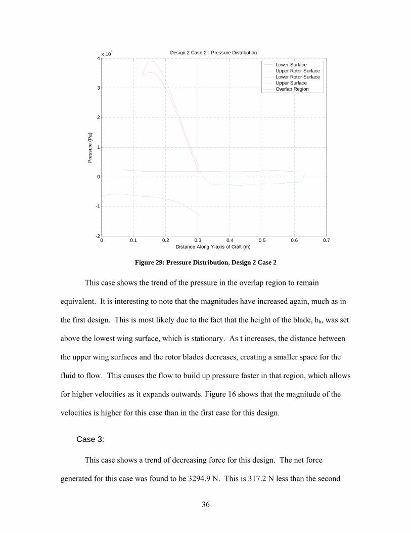
Case 3:
This case shows a trend of decreasing force for this design. The net force
generated for this case was found to be 3294.9 N. This is 317.2 N less than the second
36
case and 348 N less than the first case. Comparing Figure 32 to Figure 31, it can be seen
that the pressure along the upper surface does not drop as low as in the second case. The
pressures along the lower surface remain at almost the same level as in the second case,
which attributes for some of the loss of force in this case. When compared to Figure 30, it
is easy to see the smaller differences in pressure between the upper and lower surfaces in
this case than in the first case.
0 0.1 0.2 0.3 0.4 0.5 0.6 0.7-2
-1
0
1
2
3
4
5x 10
4 Design 2 Case 3 : Pressure Distribution
Distance Along Y-axis of Craft (m)
Pre
ssur
e (P
a)
Lower SurfaceUpper Rotor SurfaceLower Rotor SurfaceUpper SurfaceOverlap Region
Figure 30: Pressure Distribution, Design 2 Case 3
This case continues to reiterate the trend of the equivalent pressure magnitudes in
the overlap region. This continues to negate any forces from the region affecting the
overall lift forces significantly. The pressures on the upper surface of the rotor blades
also remained nearly equivalent to those in the previous cases of this design. This case
proves no significant developments in lift generation.
37
Design 3
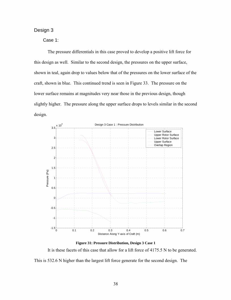
Case 1:
The pressure differentials in this case proved to develop a positive lift force for
this design as well. Similar to the second design, the pressures on the upper surface,
shown in teal, again drop to values below that of the pressures on the lower surface of the
craft, shown in blue. This continued trend is seen in Figure 33. The pressure on the
lower surface remains at magnitudes very near those in the previous design, though
slightly higher. The pressure along the upper surface drops to levels similar in the second
design.
0 0.1 0.2 0.3 0.4 0.5 0.6 0.7-1.5
-1
-0.5
0
0.5
1
1.5
2
2.5
3
3.5x 10
4 Design 3 Case 1 : Pressure Distribution
Distance Along Y-axis of Craft (m)
Pre
ssur
e (P
a)
Lower SurfaceUpper Rotor SurfaceLower Rotor SurfaceUpper SurfaceOverlap Region
Figure 31: Pressure Distribution, Design 3 Case 1
It is these facets of this case that allow for a lift force of 4175.5 N to be generated.
This is 532.6 N higher than the largest lift force generate for the second design. The
38
pressure reduction along the Coanda wing surface and the increased pressure below the
craft produce enough lift force to support a craft of 40919.9 kg. This is a significant
increase from the previous design.
It seems that the elimination of the channels in the design allow for more flow to
move through the plenum chamber and to the pressure cushion below the craft. The flow
around the Coanda wing surface does not significantly increase for this design, but the
effects of the lowered pressure are evident.
This case also continues the trend of equivalent pressures in the overlap region.
As with the cases in the second design, these pressures have little effect on the forces
generated due to negating each other. The pressure on the upper surface of the rotor
blades also remains at a similar level as the cases of the second design.
Case 2: The results from this case were similar to the first case of this design. Analysis
shows that this case produces a positive lift force as well. However, the lift force in this
case proved to be higher than in the first case for this design, with a lift force of 4822.2 N,
a significant increase of 646.7 N over the first case. A comparison of Figures 32 and 33
shows that along the upper surface both cases share the same pattern of a high pressure
region in the overlap region which quickly drops in pressure and goes below the
magnitude of the pressure of the lower surface at a point 0.31 along the Y axis of the craft.
This is slightly sooner than the previous case and would contribute a small amount of
force.
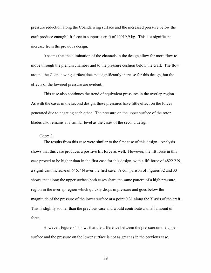
However, Figure 34 shows that the difference between the pressure on the upper
surface and the pressure on the lower surface is not as great as in the previous case.
39
Additionally, the pressure on the lower surface remains at a lower magnitude in this case
than it did in the first case. Yet, this case still produced a higher lift force.
0 0.1 0.2 0.3 0.4 0.5 0.6 0.7-2
-1
0
1
2
3
4x 10
4 Design 3 Case 2 : Pressure Distribution
Distance Along Y-axis of Craft (m)
Pre
ssur
e (P
a)
Lower SurfaceUpper Rotor SurfaceLower Rotor SurfaceUpper SurfaceOverlap Region
Figure 32: Pressure Distribution, Design 3 Case 2
The reason for the increase in the force is seen in the overlap region. This case
detracts from the previous trend of equivalent forces on the lower surface of the rotor
blades, in red, and the pressure on the upper surface of the Coanda wing that falls in the
overlap region. The pressure on the Coanda wing surface drops significantly faster than
in the previous case. This drop in pressure allows the high pressure below the rotor
blades to generate a large force addition.
The pressure on the upper surface of the rotor blade follows previous trends and
remains at previous values. The continuation of this trend and the deviation from the
40
trend in the overlap region allows this case to generate much higher lift forces the
previously observed.
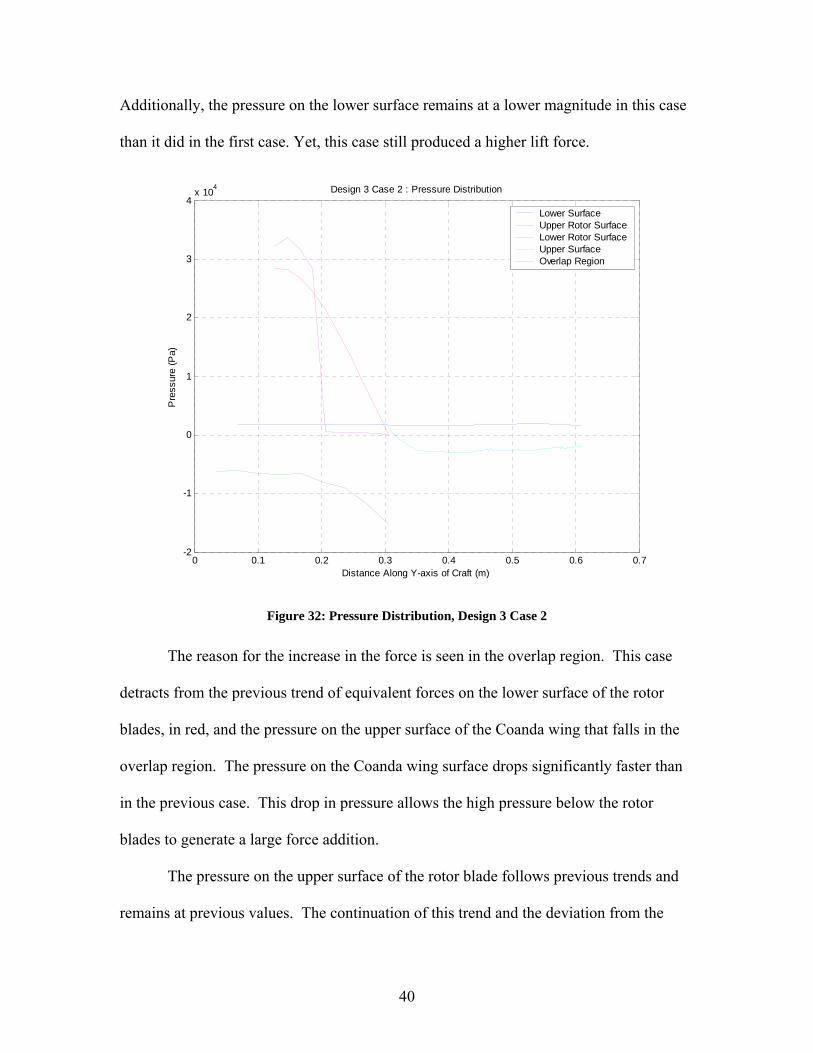
Case 3: This case again deviates from the previous trend of equivalent forces in the
overlap region. Figure 35 shows how the pressure on the Coanda wing surface in the
overlap region, seen in purple, drops even quicker than in the previous case. This result
coupled with similar results in the other areas enables this case to generate a lift force of
5388.8 N, an increase of 566.6 N over the second case of this design.
0 0.1 0.2 0.3 0.4 0.5 0.6 0.7-1.5
-1
-0.5
0
0.5
1
1.5
2
2.5
3
3.5x 10
4 Design 3 Case 3 : Pressure Distribution
Distance Along Y-axis of Craft (m)
Pre
ssur
e (P
a)
Lower SurfaceUpper Rotor SurfaceLower Rotor SurfaceUpper SurfaceOverlap Region
Figure 33: Pressure Distribution, Design 3 Case 3
The pressures along the upper and lower surfaces, blue and teal respectively,
follow all the previous trends where the pressure drops over the Coanda wing surface
allowing the pressure cushion to generate positive lift. The magnitude of the pressure on
41
the upper surface of the rotor blades remains at values similar to those seen in the
previous cases and designs. This allows the pressure on the lower surface of the rotor
blades to take advantage of the shard drop in pressure in the overlap region and generate
significant lift.
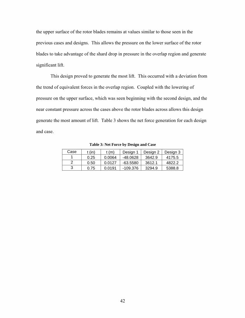
This design proved to generate the most lift. This occurred with a deviation from
the trend of equivalent forces in the overlap region. Coupled with the lowering of
pressure on the upper surface, which was seen beginning with the second design, and the
near constant pressure across the cases above the rotor blades across allows this design
generate the most amount of lift. Table 3 shows the net force generation for each design
and case.
Table 3: Net Force by Design and Case
Case t (in) t (m) Design 1 Design 2 Design 3 1 0.25 0.0064 -48.0628 3642.9 4175.5 2 0.50 0.0127 -63.5580 3612.1 4822.2 3 0.75 0.0191 -109.376 3294.9 5388.8
42
Conclusions and Recommendations
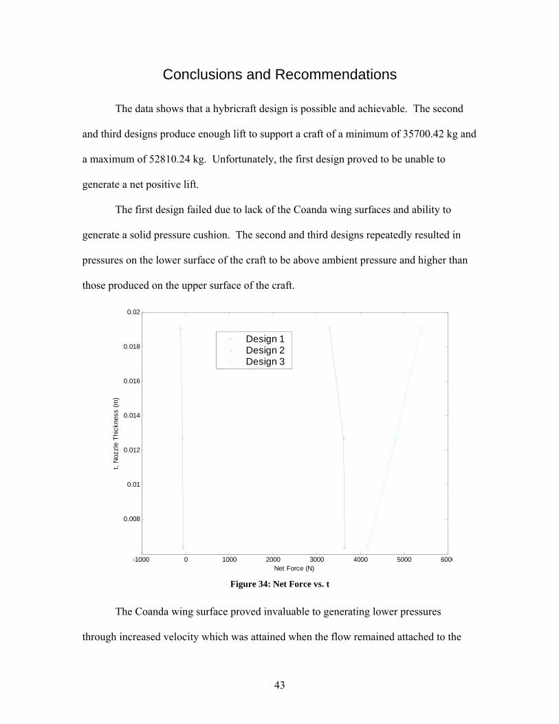
The data shows that a hybricraft design is possible and achievable. The second
and third designs produce enough lift to support a craft of a minimum of 35700.42 kg and
a maximum of 52810.24 kg. Unfortunately, the first design proved to be unable to
generate a net positive lift.
The first design failed due to lack of the Coanda wing surfaces and ability to
generate a solid pressure cushion. The second and third designs repeatedly resulted in
pressures on the lower surface of the craft to be above ambient pressure and higher than
those produced on the upper surface of the craft.
-1000 0 1000 2000 3000 4000 5000 6000
0.008
0.01
0.012
0.014
0.016
0.018
0.02
Net Force (N)
t, N
ozzl
e Th
ickn
ess
(m)
Design 1Design 2Design 3
Figure 34: Net Force vs. t
The Coanda wing surface proved invaluable to generating lower pressures
through increased velocity which was attained when the flow remained attached to the
43
surface. However, the Coanda nozzle seems to have had little affect on the flow field that
was generated around the craft. Figure 36 shows a graph of the results for each case. It
shows how with increasing t there is no significant visible trend.
For the first and second design there is a slight reduction in net force, more
significantly for the second design than in the first. The third design is the only one to
show an increase in net force with increasing t. As discussed before, this was due to a
drop in the pressure in the overlap region. From the given data it is unlikely that the
thickness of the Coanda nozzles has much affect on the flow development.
However, this study was too broad to bring about any real optimization of an
operable hybricraft design. A closer look needs to be taken in two areas. The first is the
Coanda wing and just how much lift one could generate with such a curved surface. The
second area is to look at the nozzles and how they can be adjusted to add to the air curtain
and pressure cushion below the craft. If they can be adjusted to direct more flow into the
pressure cushion and air curtain regions, it is possible that more lift could be generated.
It is also possible that the nozzles could have affects as to the stability of the craft which
have not been investigated.
An in depth study of these areas may lead to more optimized designs for this craft,
and the production of the flow needed to support the craft. Additionally, the height above
ground could be a key factor in generating stable pressure cushions. The height of the
craft above ground and its stability at maintaining flight above certain heights would be
highly useful to designing an operable hybricraft.
A closer look may also need to be taken at the CFD solver and the case setup. As
with any computational element there may be errors in the model which do not accurately
44
capture the flow. This may be easier to do if a design is tested with physical experiments
and the data compared to the CFD model. While the grids used shows consistent data
and the residuals converged to an acceptable level, the possibility for deviance from
actual flow still exists and is highly likely.
This study gives some insight as where to start as to developing a working
hybricraft. This study shows the lift can be generated by such a craft and does indeed
warrant further study. There are still the questions of stability and control as well as anti-
torque for the rotor blades and the integration of these aspects into a fully functional craft.
It is recommended that further study into the hybricraft principles be conducted to
analyze the further aspects of this possibility.
45
Appendix A
Preliminary Study of a Skirtless Hovercraft
46
Abstract
The intended purpose of this preliminary study was to look at the fluid flow of air
in and around a purposed skirtless hovercraft design. The concept was created by
William Walter in his Hybricraft Primer. The idea is to use blades to generate a
downflow of air (much like a helicopter) into and around a body. The body is specially
shaped to generate flow through Coanda Nozzles; nozzles that use the Coanda effect to
direct air towards the center and below the craft to maintain an air cushion.
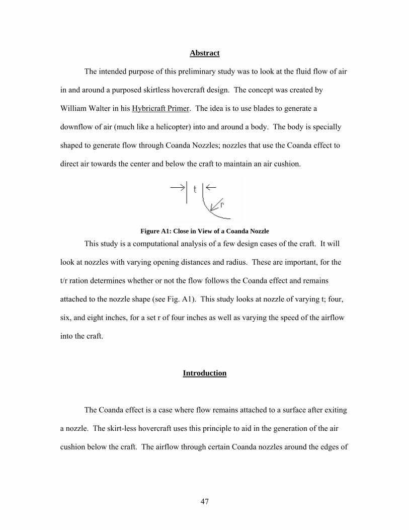
Figure A1: Close in View of a Coanda Nozzle
This study is a computational analysis of a few design cases of the craft. It will
look at nozzles with varying opening distances and radius. These are important, for the
t/r ration determines whether or not the flow follows the Coanda effect and remains
attached to the nozzle shape (see Fig. A1). This study looks at nozzle of varying t; four,
six, and eight inches, for a set r of four inches as well as varying the speed of the airflow
into the craft.
Introduction
The Coanda effect is a case where flow remains attached to a surface after exiting
a nozzle. The skirt-less hovercraft uses this principle to aid in the generation of the air
cushion below the craft. The airflow through certain Coanda nozzles around the edges of
47
the craft are designed to direct the flow to the center and below the craft thereby
maintaining a proper air cushion.
The Hybricraft Primer discusses the ideas of William Walter and includes a US
Patent for his design. This study seeks to confirm the ideas within the Hybricraft Primer
and determine the feasibility of such a craft. To do this five cases were set up to be used
in a computational fluid dynamics solver, in this case FLUENT. Each case was first
generated in Gridgen and a grid developed to capture the flow.
The five cases varied the t/r for the nozzles at the edge of the craft, those most
important to maintaining air below the craft. The cases also saw changes in the height of
the helicopter blades, modeled as velocity-inlet boundary conditions, as well as the
opening for which air was to enter the Plenum Chamber of the craft. The flow speed was
set to 50m/s for the first cases varied to 20m/s and 100m/s to look at the effect of a the air
speed into the chamber on the flow field.
The airflow was required to enter the plenum chamber of the craft prior reaching
the nozzles at the bottom of the craft. This generated some interesting vortices in the
when the solver was run in the steady case. This called for the implementation of some
ad hoc unsteady cases. These cases were run for 0.1 seconds and the residuals went to a
convergence of 0.0001.
48
Grid Description and Flow Solver
The grid for each case was generated in Gridgen software. A database was first
built to specifications and later modified to fit the different cases being used in the
analysis of the craft. Following the generation of the database six domains were
constructed. Due to the nature of the flow field and the attempt to model the Coanda
effect, the cases needed to accommodate the fact that a viscous model would be used.
For the domains around the nozzles and the majority of the craft structure a very fine
structured grid was generated using a hyperbolic extrusion method. These grids are
designed to capture the viscous boundary layer and any viscous effects that would
develop along the surface of the faces.
The initially spacing for these boundary layers was initially arbitrarily set to a
significantly small value of 0.001 as an initial guess. This is based on a general Reynolds
number for flow speeds of 50m/s. To be more accurate, the laminar grids should be
developed around each body with initial spacing specific for those bodies dimensions and
the speeds at those points. Due to the general nature of this analysis, these were not
constructed.
The remainder of the grid was made to be an unstructured gird for ease of
generation and the fact that the majority of the flow in those areas could easily be
modeled with an unstructured grid. Table A1 shows a table of each cases grid and their
dimensions. There are only four girds listed since one of the grids was a modified
version of Case 3, denoted as 3b.
49
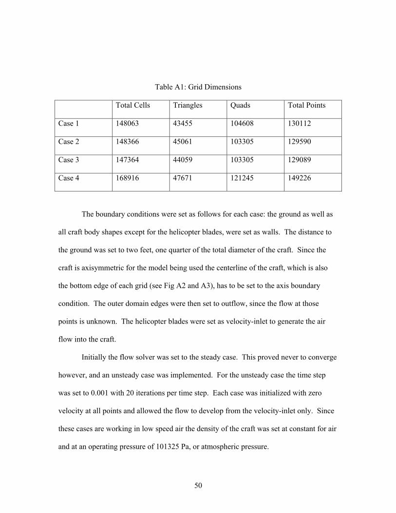
Table A1: Grid Dimensions
Total Cells Triangles Quads Total Points
Case 1 148063 43455 104608 130112
Case 2 148366 45061 103305 129590
Case 3 147364 44059 103305 129089
Case 4 168916 47671 121245 149226
The boundary conditions were set as follows for each case: the ground as well as
all craft body shapes except for the helicopter blades, were set as walls. The distance to
the ground was set to two feet, one quarter of the total diameter of the craft. Since the
craft is axisymmetric for the model being used the centerline of the craft, which is also
the bottom edge of each grid (see Fig A2 and A3), has to be set to the axis boundary
condition. The outer domain edges were then set to outflow, since the flow at those
points is unknown. The helicopter blades were set as velocity-inlet to generate the air
flow into the craft.
Initially the flow solver was set to the steady case. This proved never to converge
however, and an unsteady case was implemented. For the unsteady case the time step
was set to 0.001 with 20 iterations per time step. Each case was initialized with zero
velocity at all points and allowed the flow to develop from the velocity-inlet only. Since
these cases are working in low speed air the density of the craft was set at constant for air
and at an operating pressure of 101325 Pa, or atmospheric pressure.
50

The only boundary conditions that were set were the velocity-inlet. These were
set using the magnitude and direction option. The flow speed was tested at speeds of
20m/s, 50m/s, and 100m/s, all in the axial direction only. All cases were taken as laminar
cases, though a K-ε model was run just to see the outcome, no data was captured from the
turbulent case. Additionally, the only change that occurred to the solver were a few cases
where the relaxation parameters were changed on the pressure and momentum. These
can be seen in Figures A7 and A8.
All cases were set to 2d double precision solver. The equations of motion were
segregated and used an axisymmteric option.
Results
Figures A5 and A6 show the initial steady cases that were run on the first case.
Figure A5, which shows the axial velocity vectors shows the development of a vortex in
the plenum chamber above the Coanda nozzles. This vortex causes many problems for
the nozzles by not allowing the flow to directly exit and follow the curvature of the
nozzles. This is more easily seen in Figure A6. This shows the vectors magnitude at the
nozzle itself. The key note is the fact that the flow is actually reversed along the center
nozzle and not flowing out towards the ground at that point. These figures show the flow
at speeds of 50m/s only.
Case 2 was also run at steady flow but with a t of six inches, for a t/r of 1.5. Also
the opening into the plenum chamber was greatly increased. Figures A9, A10, and A11
show the variation in velocity from 20m/s, 50m/s, and 100m/s respectively. Again the
51
vortex forms in the plenum chamber causing flow to reverse along the Coanda nozzles,
thereby not causing the effect desired. This also reduces the pressure of the air cushion
below the craft.
Case 3 was for t/r of 1.5 with the greatly increased inlet area as well. However,
this case was run unsteady at 100m/s. 100m/s was used in the unsteady cases since it
seemed to remove the vortex that was formed inside the plenum chamber, as can be seen
in Figure A12. For speeds less than 100m/s, the vortex developed even in the unsteady
cases. Looking at Figure A13 shows the noticeable change in the flow field due to the
removal of the vortex. The flow actually manages to follow the outer edge of the nozzle.
However, it seems the flow still reverses at the upper tip of the nozzle but then manages
to follow the inner edge as well. Also, the flow comes to a separation point and then
flows out and away from the craft, this occurs at about the midway point on the inner
curve of the outer nozzle.
Figure A14 shows an up close view of the inlet conditions. This is interesting due
to the large vortex that is created by the velocity-inlet. This vortex may cause problems
with the flow over the outer edge of the craft. This vortex is also present in the previous
figures. It is possible that a mass flow boundary condition may better model the flow in
this area. Figure A15 is a pressure contour map to see the pressures below the craft.
However, the contour may reveal errors in the flow analysis due to the negative static
pressures around the outside of the craft. This brings the validity of the results into
question.
Figures A16 – A19 are the data for Case 3b. This case is the same grid as Case 3,
except with the blades (velocity-inlet) lowered to within three inches of the craft.
52
Looking at Figures A16 and A17, there seems to be little difference in the flow due to
this fact. When compared to Figures A12 and A13 there is not any noticeable differences.
Figure A18 shows the major different, that being at the inlet. The vortex affects the flow
around the entry edge of the outer surface of the craft. The flow is slower than in Case 3
at that point.
Case 4 is a case with t/r = 2 and the addition of a flow splitter at the entrance of
the inlet. This splitter is intended to direct flow from the inlet along the inner edge of the
outer surface and hopefully maintain that flow to induce the Coanda effect at the nozzle
later. This however proved to be not very successful. It can be seen in Figure A21 that
the flow at the Coanda nozzle is not much different from Case 3. Also, while the vortex
at the inlet seems to have reduced some from Case 3, the flow that goes by the splitter
seems only to slow down and has little effect on the later development of the flow.
Conclusions and Recommendations
The most significant conclusion is that the Coanda nozzle have not worked for
these flow and design conditions. This study also reveals the necessity for the use of an
unsteady solver and the probably use of inlet velocities of 100m/s or greater. The grids
also need to be further refined to capture the flow properties at the bodies more
effectively.
The pressure data also suggest a possible need to expand the area around the craft
to capture more accurate data of the flow field. Additionally, due to the ineffectiveness
of the chosen t/r, a further study of various t/r’s should be conducted to find the optimum
53
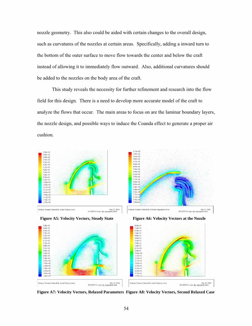
nozzle geometry. This also could be aided with certain changes to the overall design,
such as curvatures of the nozzles at certain areas. Specifically, adding a inward turn to
the bottom of the outer surface to move flow towards the center and below the craft
instead of allowing it to immediately flow outward. Also, additional curvatures should
be added to the nozzles on the body area of the craft.
This study reveals the necessity for further refinement and research into the flow
field for this design. There is a need to develop more accurate model of the craft to
analyze the flows that occur. The main areas to focus on are the laminar boundary layers,
the nozzle design, and possible ways to induce the Coanda effect to generate a proper air
cushion.
Figure A5: Velocity Vectors, Steady State Figure A6: Velocity Vectors at the Nozzle
Figure A7: Velocity Vectors, Relaxed Parameters Figure A8: Velocity Vectors, Second Relaxed Case
54
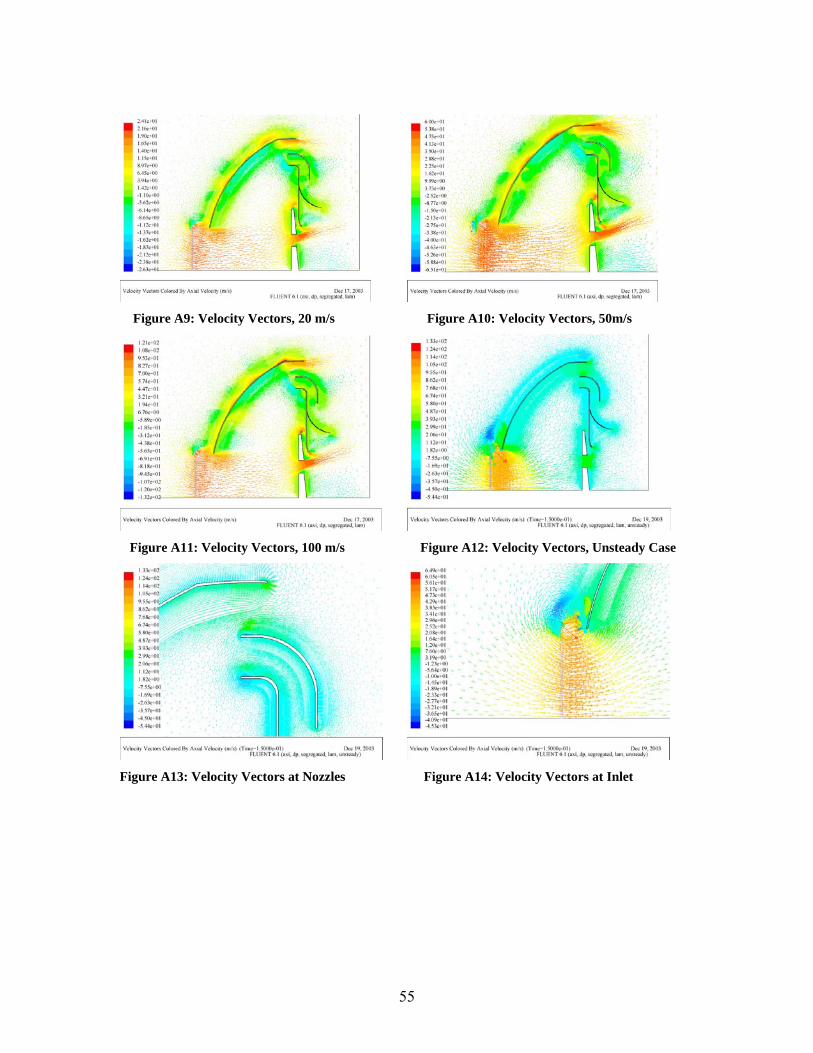
Figure A9: Velocity Vectors, 20 m/s Figure A10: Velocity Vectors, 50m/s
Figure A11: Velocity Vectors, 100 m/s Figure A12: Velocity Vectors, Unsteady Case
Figure A13: Velocity Vectors at Nozzles Figure A14: Velocity Vectors at Inlet
55
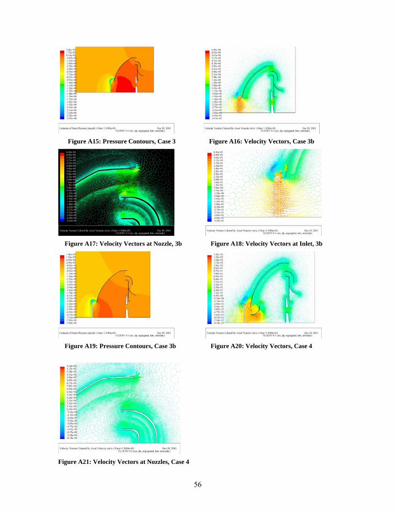
Figure A15: Pressure Contours, Case 3 Figure A16: Velocity Vectors, Case 3b
Figure A17: Velocity Vectors at Nozzle, 3b Figure A18: Velocity Vectors at Inlet, 3b
Figure A19: Pressure Contours, Case 3b Figure A20: Velocity Vectors, Case 4
Figure A21: Velocity Vectors at Nozzles, Case 4
56
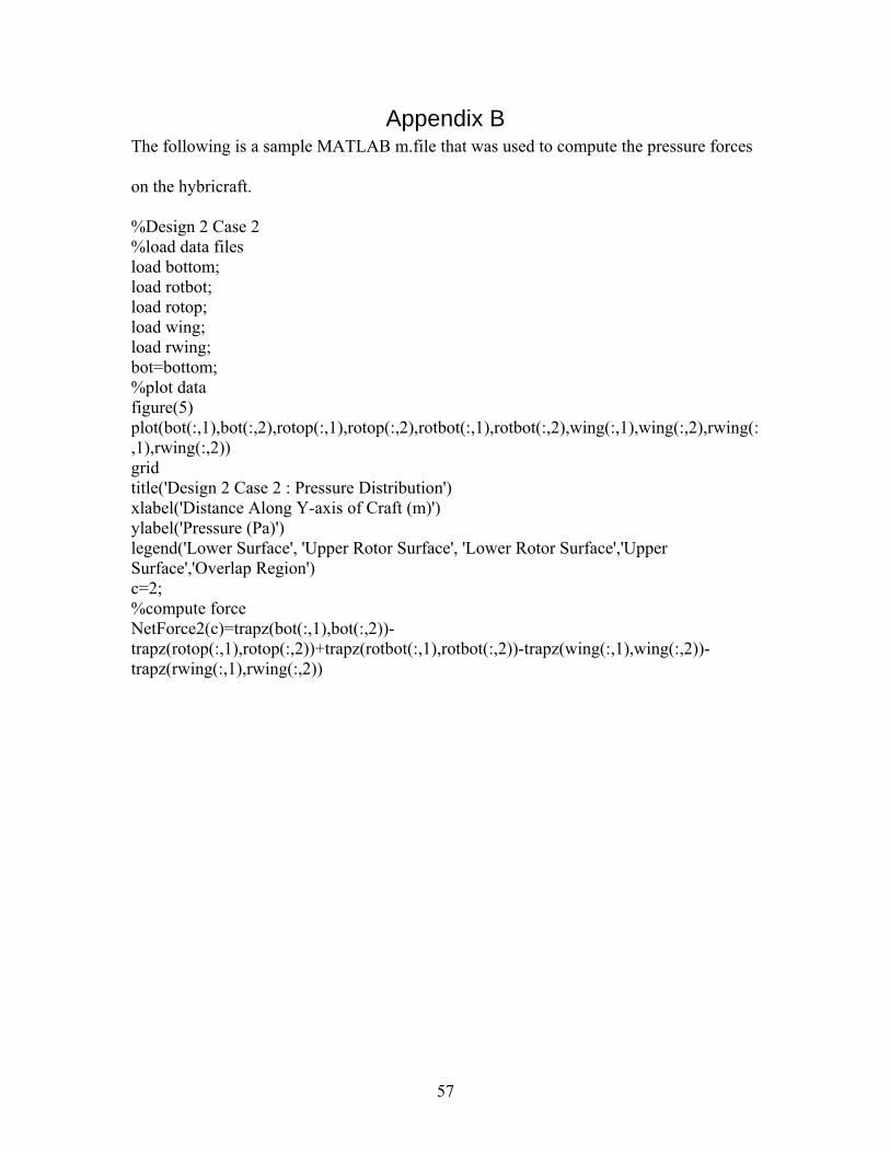
Appendix B The following is a sample MATLAB m.file that was used to compute the pressure forces
on the hybricraft.
%Design 2 Case 2 %load data files load bottom; load rotbot; load rotop; load wing; load rwing; bot=bottom; %plot data figure(5) plot(bot(:,1),bot(:,2),rotop(:,1),rotop(:,2),rotbot(:,1),rotbot(:,2),wing(:,1),wing(:,2),rwing(:,1),rwing(:,2)) grid title('Design 2 Case 2 : Pressure Distribution') xlabel('Distance Along Y-axis of Craft (m)') ylabel('Pressure (Pa)') legend('Lower Surface', 'Upper Rotor Surface', 'Lower Rotor Surface','Upper Surface','Overlap Region') c=2; %compute force NetForce2(c)=trapz(bot(:,1),bot(:,2))-trapz(rotop(:,1),rotop(:,2))+trapz(rotbot(:,1),rotbot(:,2))-trapz(wing(:,1),wing(:,2))-trapz(rwing(:,1),rwing(:,2))
57
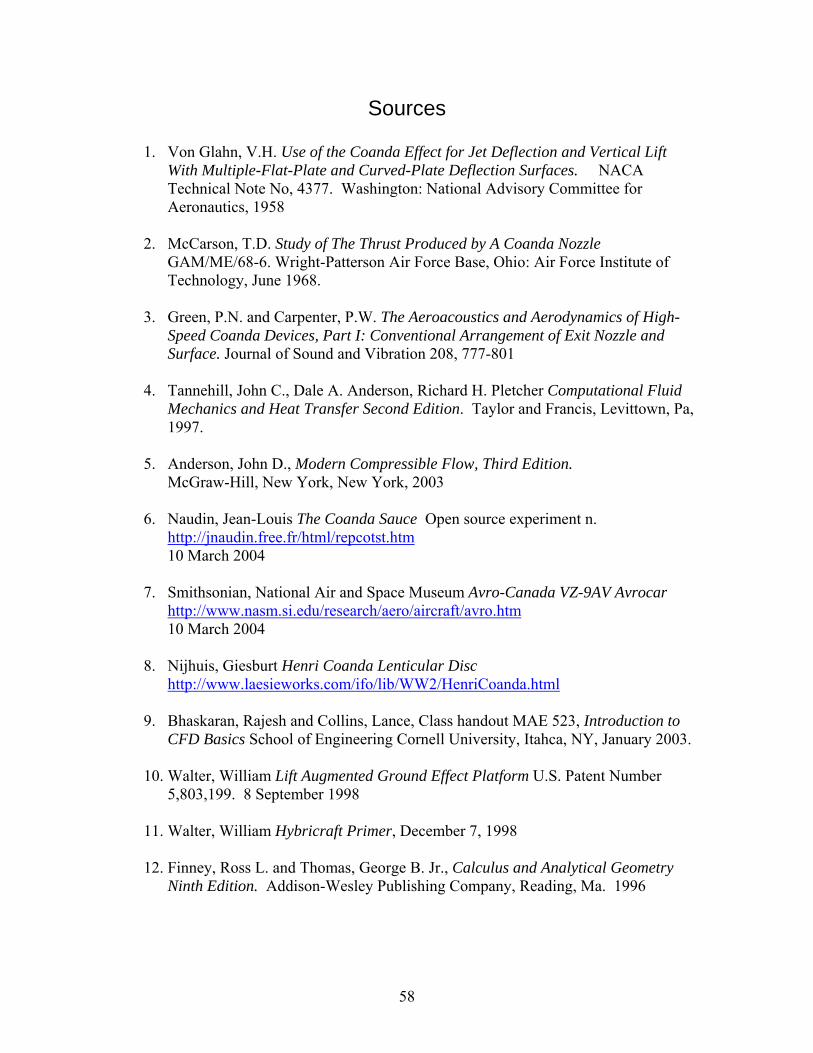
Sources
1. Von Glahn, V.H. Use of the Coanda Effect for Jet Deflection and Vertical Lift With Multiple-Flat-Plate and Curved-Plate Deflection Surfaces. NACA Technical Note No, 4377. Washington: National Advisory Committee for Aeronautics, 1958
2. McCarson, T.D. Study of The Thrust Produced by A Coanda Nozzle
GAM/ME/68-6. Wright-Patterson Air Force Base, Ohio: Air Force Institute of Technology, June 1968.
3. Green, P.N. and Carpenter, P.W. The Aeroacoustics and Aerodynamics of High-
Speed Coanda Devices, Part I: Conventional Arrangement of Exit Nozzle and Surface. Journal of Sound and Vibration 208, 777-801
4. Tannehill, John C., Dale A. Anderson, Richard H. Pletcher Computational Fluid
Mechanics and Heat Transfer Second Edition. Taylor and Francis, Levittown, Pa, 1997.
5. Anderson, John D., Modern Compressible Flow, Third Edition.
McGraw-Hill, New York, New York, 2003
6. Naudin, Jean-Louis The Coanda Sauce Open source experiment n. http://jnaudin.free.fr/html/repcotst.htm 10 March 2004
7. Smithsonian, National Air and Space Museum Avro-Canada VZ-9AV Avrocar
http://www.nasm.si.edu/research/aero/aircraft/avro.htm 10 March 2004
8. Nijhuis, Giesburt Henri Coanda Lenticular Disc http://www.laesieworks.com/ifo/lib/WW2/HenriCoanda.html
9. Bhaskaran, Rajesh and Collins, Lance, Class handout MAE 523, Introduction to
CFD Basics School of Engineering Cornell University, Itahca, NY, January 2003.
10. Walter, William Lift Augmented Ground Effect Platform U.S. Patent Number 5,803,199. 8 September 1998
11. Walter, William Hybricraft Primer, December 7, 1998
12. Finney, Ross L. and Thomas, George B. Jr., Calculus and Analytical Geometry
Ninth Edition. Addison-Wesley Publishing Company, Reading, Ma. 1996
58
Vitae Ensign Edward A. Kelleher graduated from Conestoga High School in Berwyn,
Pennsylvania in June of 1999. He attended Cornell University School of Engineering in
August 1999, Ithaca, NY, and enrolled in the Naval Reserve Officer Training Corps. He
graduated in May 2003 with a Bachelor of Science in Mechanical Engineering and was
granted a commission in the United States Naval Reserve.
Upon entering Active duty ENS Kelleher was selected for the Immediate
Graduate Education Program (IGEP) and entered the Air Force Institute of Technology
School of Engineering and Management. He moved to Wright-Patterson Air Force Base,
Dayton, OH in June of 2003. There he worked towards a Masters of Science in
Aeronautical Engineering. Upon graduation he will be assigned to NAS Pensacola to
enter Aviation Preflight Indoctrination.
59
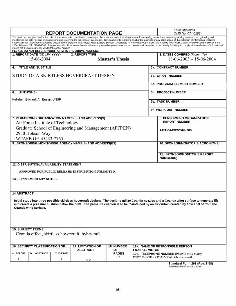
REPORT DOCUMENTATION PAGE Form Approved OMB No. 074-0188
The public reporting burden for this collection of information is estimated to average 1 hour per response, including the time for reviewing instructions, searching existing data sources, gathering and maintaining the data needed, and completing and reviewing the collection of information. Send comments regarding this burden estimate or any other aspect of the collection of information, including suggestions for reducing this burden to Department of Defense, Washington Headquarters Services, Directorate for Information Operations and Reports (0704-0188), 1215 Jefferson Davis Highway, Suite 1204, Arlington, VA 22202-4302. Respondents should be aware that notwithstanding any other provision of law, no person shall be subject to an penalty for failing to comply with a collection of information if it does not display a currently valid OMB control number. PLEASE DO NOT RETURN YOUR FORM TO THE ABOVE ADDRESS. 1. REPORT DATE (DD-MM-YYYY)
15-06-2004 2. REPORT TYPE
Master’s Thesis
3. DATES COVERED (From – To) 18-06-2003 – 15-06-2004
5a. CONTRACT NUMBER
5b. GRANT NUMBER
4. TITLE AND SUBTITLE STUDY OF A SKIRTLESS HOVERCRAFT DESIGN 5c. PROGRAM ELEMENT NUMBER
5d. PROJECT NUMBER 5e. TASK NUMBER
6. AUTHOR(S) Kelleher, Edward, A., Ensign UNSR
5f. WORK UNIT NUMBER
7. PERFORMING ORGANIZATION NAMES(S) AND ADDRESS(S) Air Force Institute of Technology Graduate School of Engineering and Management (AFIT/EN) 2950 Hobson Way WPAFB OH 45433-7765
8. PERFORMING ORGANIZATION REPORT NUMBER AFIT/GAE/ENY/04-J05
10. SPONSOR/MONITOR’S ACRONYM(S)
9. SPONSORING/MONITORING AGENCY NAME(S) AND ADDRESS(ES)
11. SPONSOR/MONITOR’S REPORT
NUMBER(S)
12. DISTRIBUTION/AVAILABILITY STATEMENT APPROVED FOR PUBLIC RELEASE; DISTRIBUTION UNLIMITED.
13. SUPPLEMENTARY NOTES 14 ABSTRACT
Initial study into three possible skirtless hovercraft designs. The designs utilize Coanda nozzles and a Coanda wing surface to generate lift and create a pressure cushion below the craft. The pressure cushion is to be maintained by an air curtain created by flow spill of from the Coanda wing surface.
15. SUBJECT TERMS Coanda effect, skirtless hovercraft, hybricraft.
16. SECURITY CLASSIFICATION OF: 19a. NAME OF RESPONSIBLE PERSON FRANKE, MILTON
a. REPORT
U
b. ABSTRACT
U
c. THIS PAGE
U
17. LIMITATION OF ABSTRACT
UU
18. NUMBER OF PAGES
70 19b. TELEPHONE NUMBER (Include area code) DEPT PHONE – 937-255-3069 Advisor e-mail
Standard Form 298 (Rev. 8-98) Prescribed by ANSI Std. Z39-18
60
Recommended