1
Ka-fu WongUniversity of Hong Kong
An Introduction to EViews 4.1 (Student version)

2
Installation
Insert the CD-ROM disc in a drive and install the program on the computer.
For most of us, accepting all defaults will work fine.
Note that you can install EViews on as many computers as you want to. However, at start, EViews will ask you to insert the CD-ROM disc.

3
Starting EViews
Work Area
May be changed with Options>File Locations>Current Data Path.
Current Data Path.
Command Area

4
Options>File Locations>Current Data Path
Current Data Path. May be changed with Options>File Locations>Current Data Path.

5
Open the Excel file containing the data(example2.XLS)
48 undated observations4 columns (OBS, X, Y, Z)3 variables: X, Y, Z

6
Enter or read data in EviewsFile > New > Workfile
1. Choose “Undated or irregular”.
2. Specify 1 and 48.
3. Click OK.
7
Enter or read data in Eviews Choose Quick>Empty Group(Edit Series)

8
Enter or read data in Eviews Key in data
9
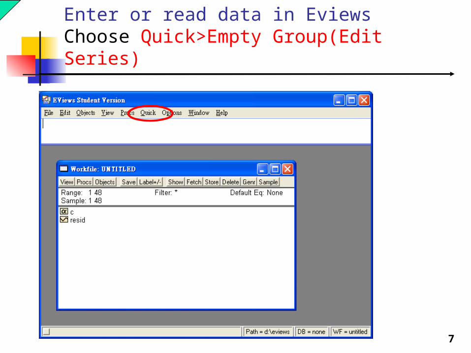
Enter or read data in Eviews Copy the data from Excel (A2:D49 together) to the Workfile
Default series names

10
Renaming the seriesFirst minimize the data sheet
Highlight ser01 and right click mouse, and choose rename

11
Rename the series (ser01 – ser04)

12
Check if the variable names has been changed

13
Save data and results frequently to avoide loss of dataFile>SaveAs
Enter example0.wf1

14
Scatterplot of X and Y
1. Highlight x and y
2. Quick > Graph > Scatter
3. Order the variables
4. click OK.

15
Scatterplot of X and Y

16
Scatterplot of X and YUse options to adjust the appearance

17
Scatterplot of X and YUse AddText to adjust the appearance

18
Use Lines/Shading to adjust the appearance

19
Scatter plot after some formatting

20
Alternative way to do scatterplot of X and Y1. Put X and Y in a group called gxygroup gxy X Y

21
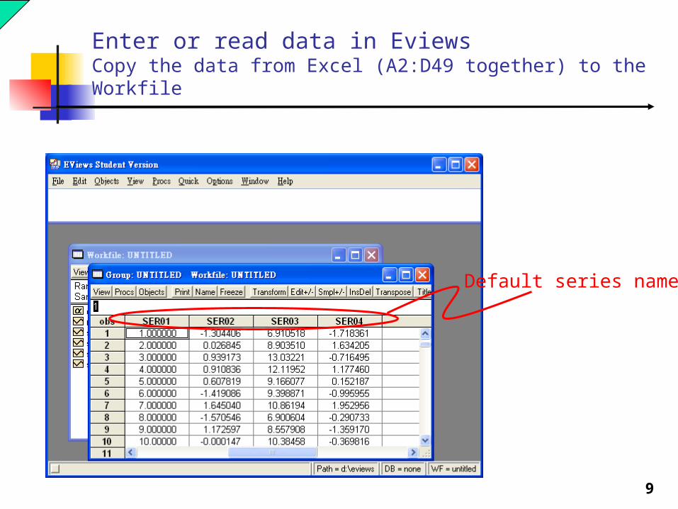
Alternative way to do scatterplot of X and Y2. Generate scatter plot using the data group of gxyfreeze(Figure21) gxy.scat
22
Alternative way to do scatterplot of X and YDouble click figure21 to view the plot

23
Scatter plot of X and Y

24
Generate a scatter plus a linear fitfreeze(Figure22) gxy.linefit
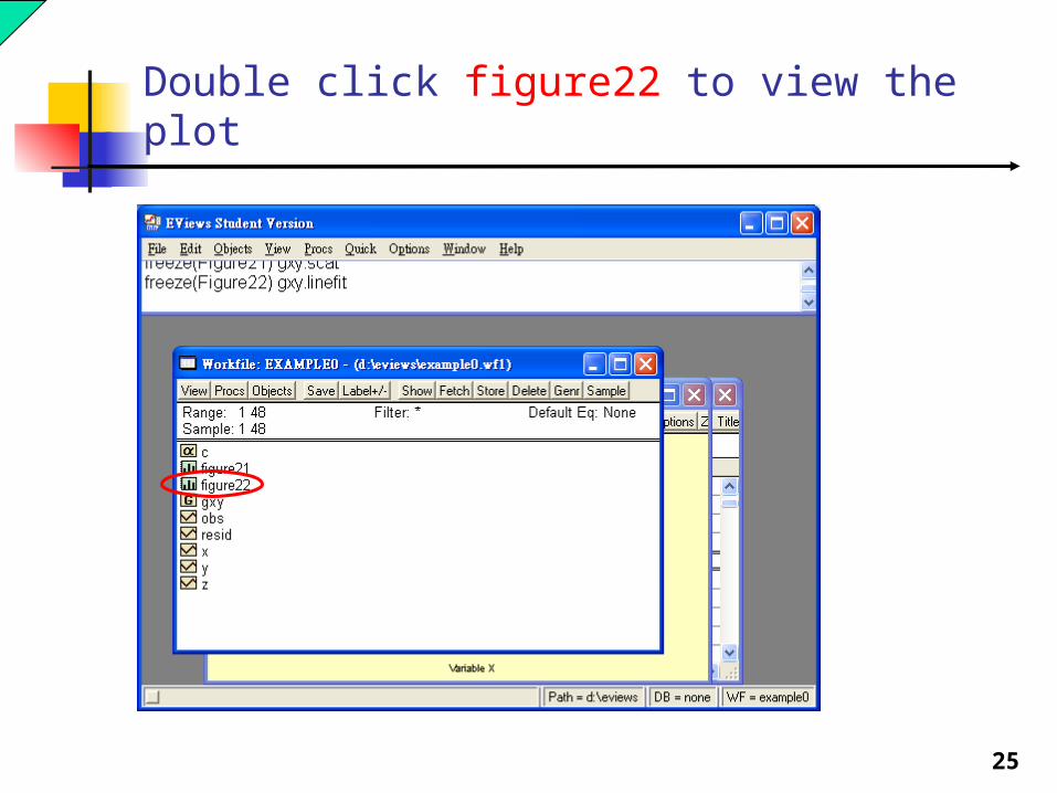
25
Double click figure22 to view the plot

26
Scatter plot with linear fit

27
Group data for scatter plotgroup gzy z y

28
Create scatter plot, save in Figure23freeze(Figure23) gzy.linefit

29
Another scatter plot (data group gzy) with linear fit

30
Run linear regression and save the results in tableA1equation tableA1.ls y c x z (Y = c + b0X + b1Z)

31
Regression results (tablea1)

32
Save all the results and dataFile > SaveAs

33
Next time, we can open the workfileFile > Open > workfile

34
We can continue to work on the data and plots…

35
End

36
Plot residuals and fitted values

37
Plot residuals and fitted values
Recommended