IE 5441 1
# 6. Comparing Alternatives
One of the main purposes of this course is to discuss how to make
decisions in engineering economy.
Let us first consider a single period case.
Suppose that there are two projects: A and B. Project A requires an
investment of HK$10K and will return in one year time HK$12K. The
other project requires HK$100K investment and returns HK$115K
next year.
Clearly, irrA = 20% and irrB = 15%.
Suppose that your MARR is 10%.
What do you do?
Shuzhong Zhang
IE 5441 2
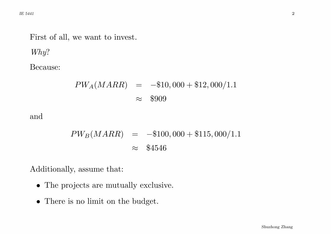
First of all, we want to invest.
Why?
Because:
PWA(MARR) = −$10, 000 + $12, 000/1.1
≈ $909
and
PWB(MARR) = −$100, 000 + $115, 000/1.1
≈ $4546
Additionally, assume that:
• The projects are mutually exclusive.
• There is no limit on the budget.
Shuzhong Zhang
IE 5441 3
According to their present value, the preference is clearly B ≻ A.
According to the IRR, A looks more attractive than B.
Which consideration makes more sense?
Let us start from the basis that:
Any investment is acceptable only when its PW under the
MARR is positive.
Shuzhong Zhang

IE 5441 4
So, we must justify the use of the additional $90,000 in Project B. In
fact B \A requires an initial investment of $90,000 and returns with
$103,000. Under the MARR its present worth is
−$90, 000 + $103, 000/1.1 ≈ $3, 636
Conclusion: The use of additional $90,000 in Project B is justified,
and so B ≻ A.
Careful: The IRR can give some misleading conclusions!
Shuzhong Zhang
IE 5441 5
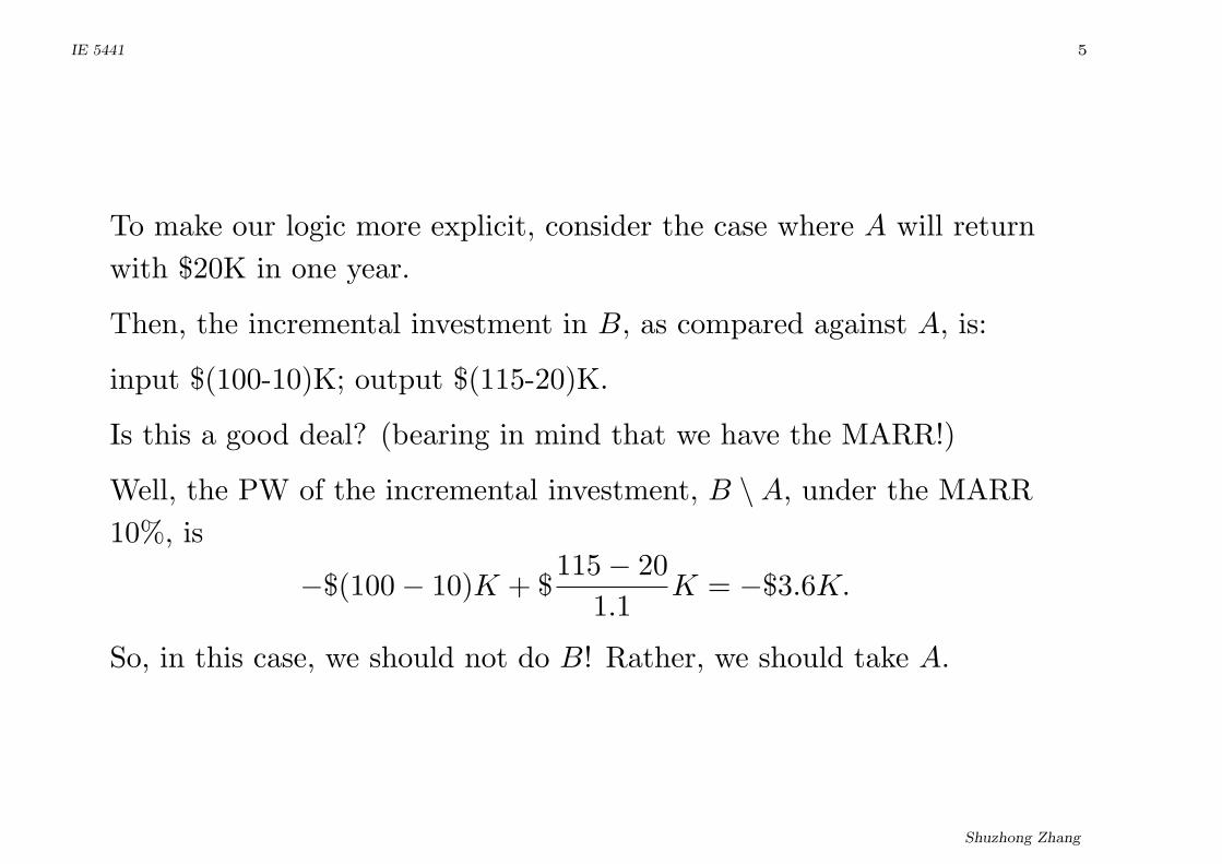
To make our logic more explicit, consider the case where A will return
with $20K in one year.
Then, the incremental investment in B, as compared against A, is:
input $(100-10)K; output $(115-20)K.
Is this a good deal? (bearing in mind that we have the MARR!)
Well, the PW of the incremental investment, B \A, under the MARR
10%, is
−$(100− 10)K + $115− 20
1.1K = −$3.6K.
So, in this case, we should not do B! Rather, we should take A.
Shuzhong Zhang
IE 5441 6
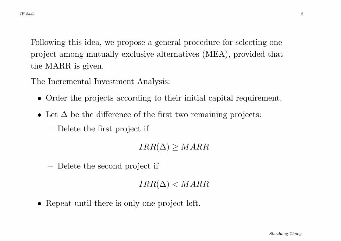
Following this idea, we propose a general procedure for selecting one
project among mutually exclusive alternatives (MEA), provided that
the MARR is given.
The Incremental Investment Analysis:
• Order the projects according to their initial capital requirement.
• Let ∆ be the difference of the first two remaining projects:
– Delete the first project if
IRR(∆) ≥ MARR
– Delete the second project if
IRR(∆) < MARR
• Repeat until there is only one project left.
Shuzhong Zhang
IE 5441 7
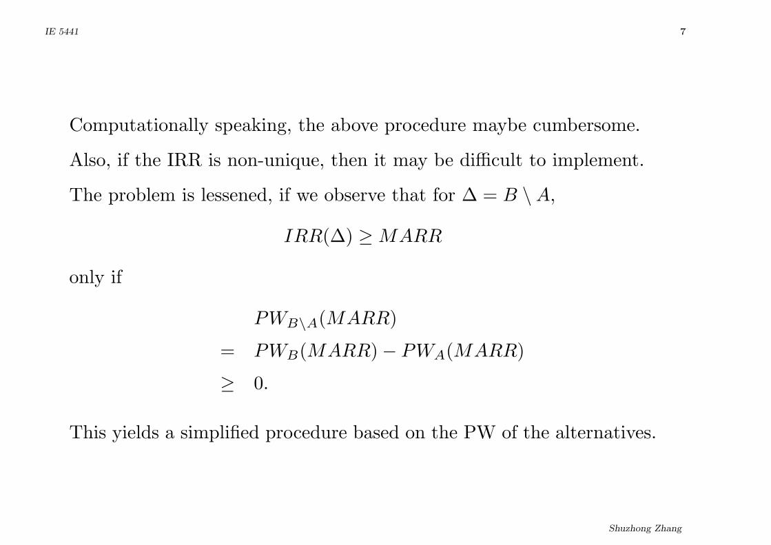
Computationally speaking, the above procedure maybe cumbersome.
Also, if the IRR is non-unique, then it may be difficult to implement.
The problem is lessened, if we observe that for ∆ = B \A,
IRR(∆) ≥ MARR
only if
PWB\A(MARR)
= PWB(MARR)− PWA(MARR)
≥ 0.
This yields a simplified procedure based on the PW of the alternatives.
Shuzhong Zhang
IE 5441 8
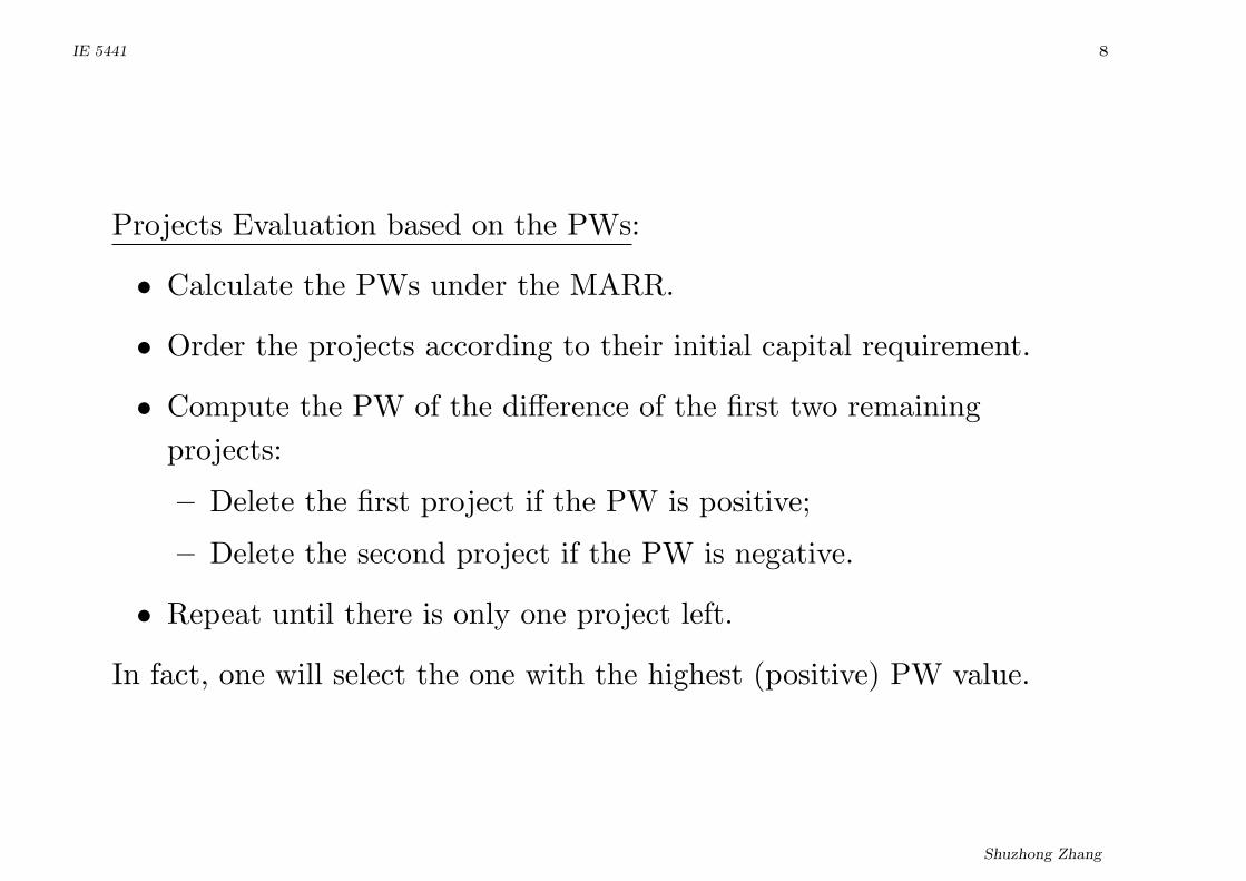
Projects Evaluation based on the PWs:
• Calculate the PWs under the MARR.
• Order the projects according to their initial capital requirement.
• Compute the PW of the difference of the first two remaining
projects:
– Delete the first project if the PW is positive;
– Delete the second project if the PW is negative.
• Repeat until there is only one project left.
In fact, one will select the one with the highest (positive) PW value.
Shuzhong Zhang
IE 5441 9
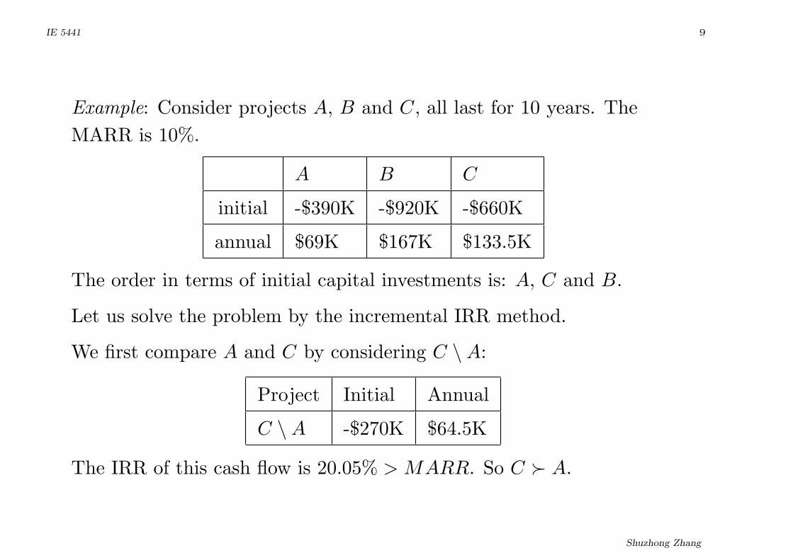
Example: Consider projects A, B and C, all last for 10 years. The
MARR is 10%.
A B C
initial -$390K -$920K -$660K
annual $69K $167K $133.5K
The order in terms of initial capital investments is: A, C and B.
Let us solve the problem by the incremental IRR method.
We first compare A and C by considering C \A:
Project Initial Annual
C \A -$270K $64.5K
The IRR of this cash flow is 20.05% > MARR. So C ≻ A.
Shuzhong Zhang
IE 5441 10
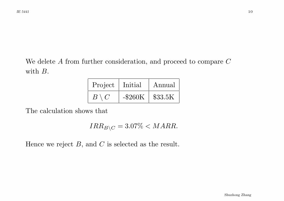
We delete A from further consideration, and proceed to compare C
with B.
Project Initial Annual
B \ C -$260K $33.5K
The calculation shows that
IRRB\C = 3.07% < MARR.
Hence we reject B, and C is selected as the result.
Shuzhong Zhang
IE 5441 11
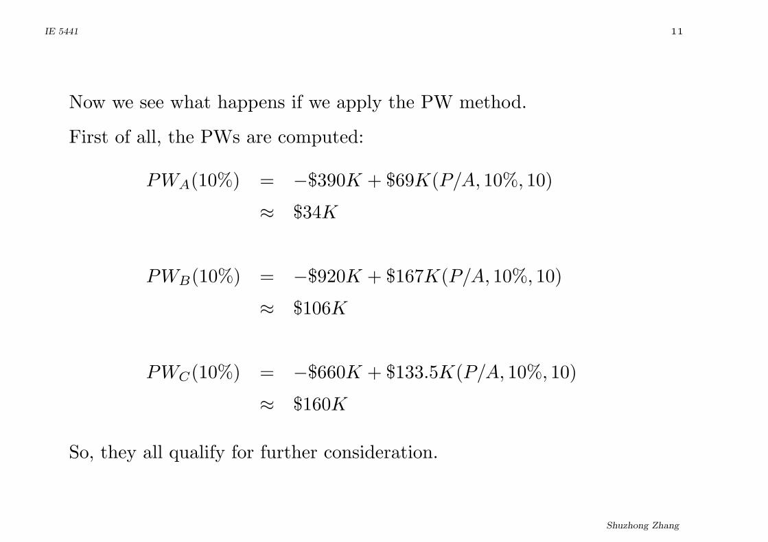
Now we see what happens if we apply the PW method.
First of all, the PWs are computed:
PWA(10%) = −$390K + $69K(P/A, 10%, 10)
≈ $34K
PWB(10%) = −$920K + $167K(P/A, 10%, 10)
≈ $106K
PWC(10%) = −$660K + $133.5K(P/A, 10%, 10)
≈ $160K
So, they all qualify for further consideration.
Shuzhong Zhang

IE 5441 12
In the increasing order of initial investment: A, C and B.
We consider C \A:PWC\A ≈ 126K > 0
Therefore we take C and delete A.
Now consider B \ C:
PWB\C ≈ −54K < 0
So, the additional budget needed for B is worse than the MARR.
Conclusion: C is most attractive under the MARR. In fact,
C ≻ B ≻ A.
Shuzhong Zhang
IE 5441 13
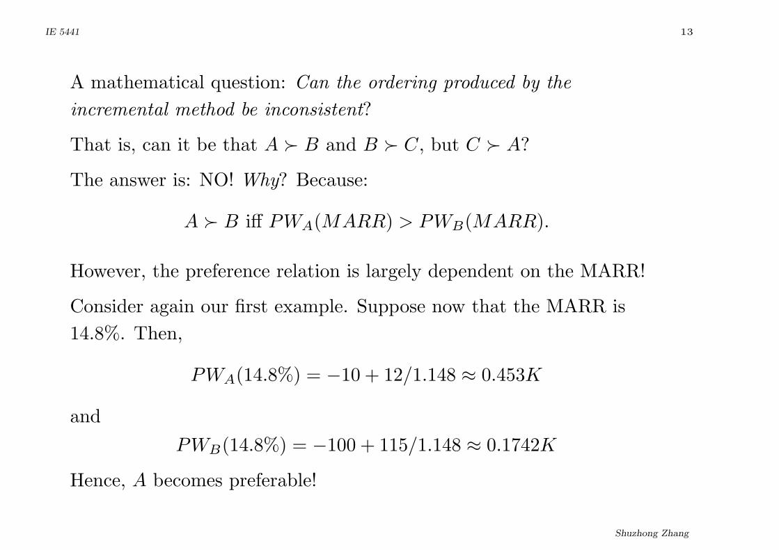
A mathematical question: Can the ordering produced by the
incremental method be inconsistent?
That is, can it be that A ≻ B and B ≻ C, but C ≻ A?
The answer is: NO! Why? Because:
A ≻ B iff PWA(MARR) > PWB(MARR).
However, the preference relation is largely dependent on the MARR!
Consider again our first example. Suppose now that the MARR is
14.8%. Then,
PWA(14.8%) = −10 + 12/1.148 ≈ 0.453K
and
PWB(14.8%) = −100 + 115/1.148 ≈ 0.1742K
Hence, A becomes preferable!
Shuzhong Zhang

IE 5441 14
Note: Of course, the evaluation based on PW is equivalent to that
based on FW or AW.
As we have seen in the first example, it is wrong to select the project
with the highest IRR.
Example: Consider 6 projects A, B, C, D, E and F . The duration for
all projects are for 10 years and their cash flows are given as follows:
Project Initial Investment Annual Profit
A -$900 $150
B -$1,500 $276
C -$2,500 $400
D -$4,000 $925
E -$5,000 $1,125
F -$7,000 $1,425
Suppose that MARR = 10%.
Shuzhong Zhang
IE 5441 15
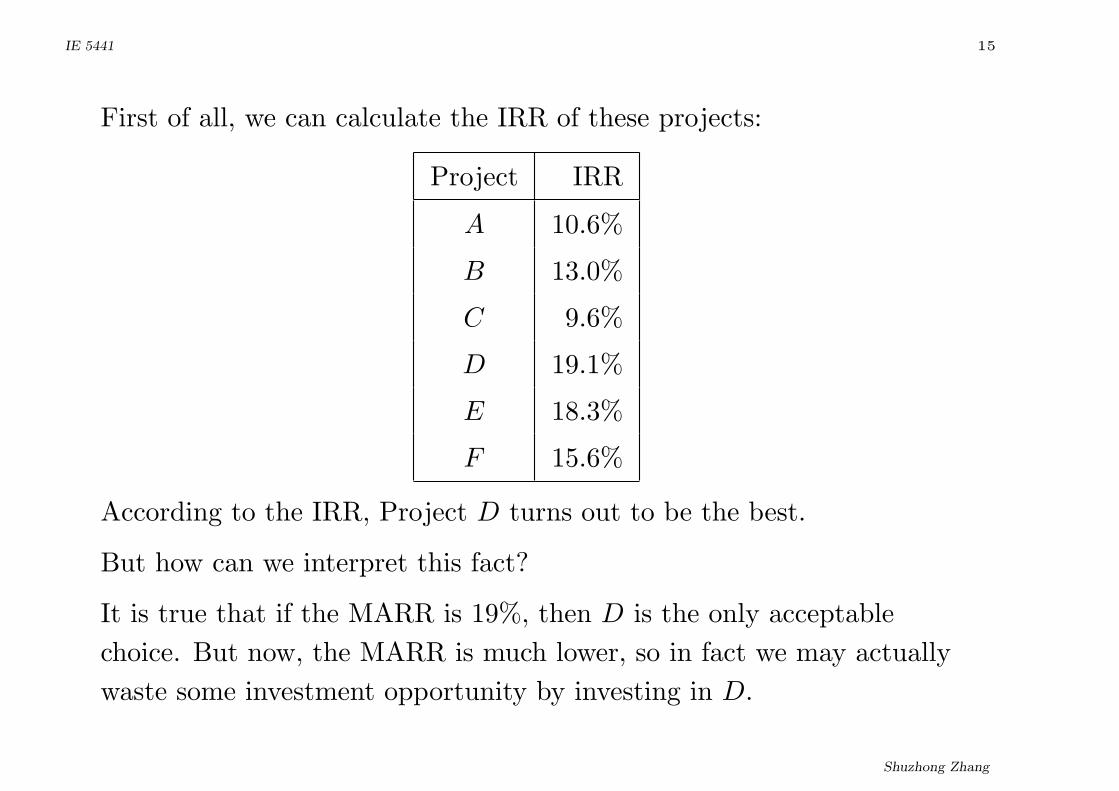
First of all, we can calculate the IRR of these projects:
Project IRR
A 10.6%
B 13.0%
C 9.6%
D 19.1%
E 18.3%
F 15.6%
According to the IRR, Project D turns out to be the best.
But how can we interpret this fact?
It is true that if the MARR is 19%, then D is the only acceptable
choice. But now, the MARR is much lower, so in fact we may actually
waste some investment opportunity by investing in D.
Shuzhong Zhang
IE 5441 16
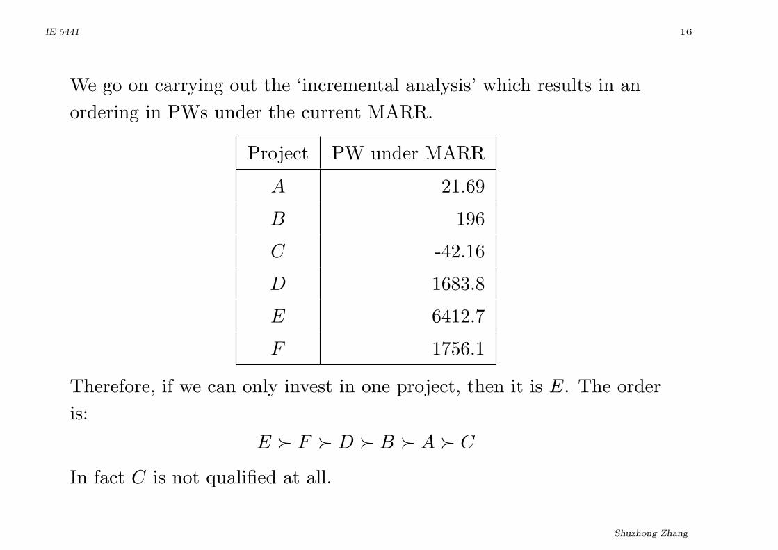
We go on carrying out the ‘incremental analysis’ which results in an
ordering in PWs under the current MARR.
Project PW under MARR
A 21.69
B 196
C -42.16
D 1683.8
E 6412.7
F 1756.1
Therefore, if we can only invest in one project, then it is E. The order
is:
E ≻ F ≻ D ≻ B ≻ A ≻ C
In fact C is not qualified at all.
Shuzhong Zhang
IE 5441 17
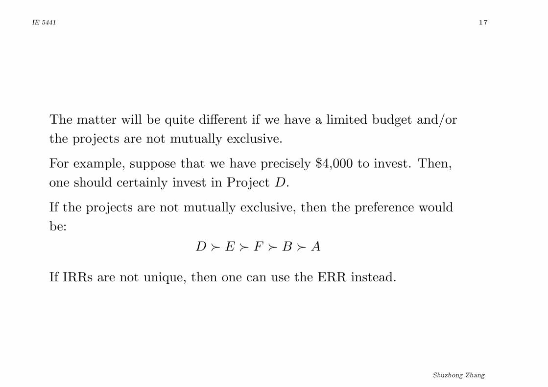
The matter will be quite different if we have a limited budget and/or
the projects are not mutually exclusive.
For example, suppose that we have precisely $4,000 to invest. Then,
one should certainly invest in Project D.
If the projects are not mutually exclusive, then the preference would
be:
D ≻ E ≻ F ≻ B ≻ A
If IRRs are not unique, then one can use the ERR instead.
Shuzhong Zhang

IE 5441 18
Comparing Alternatives (continue).
So far, we have made the following assumptions in our analysis:
• The alternatives are mutually exclusive
• The life-span of the alternatives are the same
The basic idea of the method is simple: We try to see whether any
additional cent on a more expensive project is well spent, in
comparison with the MARR.
This is termed the incremental analysis.
Shuzhong Zhang

IE 5441 19
In some applications indeed only one alternative is to be chosen.
Example: Suppose that one must install an air compressor among 4
choices for 5 years. Their respective expenses are as follows.
Project Price Annual Cost Resale Value
D1 -100K -29K 10K
D2 -140K -16.9K 14K
D3 -148.2K -14.8K 25.6K
D4 -122K -22.1K 14K
Suppose that MARR=20%.
Shuzhong Zhang

IE 5441 20
First of all, this is a cost alternatives, meaning that we need only to
see whether the benefit from any additional cost is more attractive
than the MARR or not.
From D1 to D4, the cash flow is
Price Diff Annual Saving End Value
-22K 6.9K 4K
Hence,
IRR(∆D4\D1) = 20.5%.
The investment is justified.
Shuzhong Zhang

IE 5441 21
Next we consider the incremental from D4 to D2.
Price Diff Annual Saving End Value
-18K 5.2K 0K
IRR(∆D2\D4) = 12.3%.
The additional investment is NOT justified.
Shuzhong Zhang
IE 5441 22
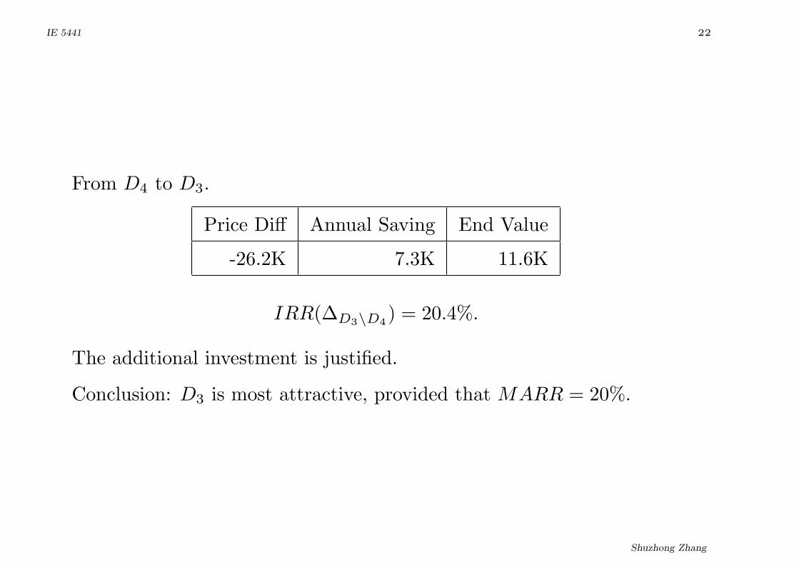
From D4 to D3.
Price Diff Annual Saving End Value
-26.2K 7.3K 11.6K
IRR(∆D3\D4) = 20.4%.
The additional investment is justified.
Conclusion: D3 is most attractive, provided that MARR = 20%.
Shuzhong Zhang

IE 5441 23
We may as well use the PWs in the analysis.
The PWs under the MARR are:
Project PW(MARR)
D1 -182.7084K
D2 -185.5148K
D3 -182.1722K
D4 -182.4657K
Therefore, the least costly alternative is D3.
It leads to the same conclusion.
Shuzhong Zhang

IE 5441 24
Example: A downtown parking center was out of capacity. Catherine
Jones, an ambitious new employee of an architectural engineering firm,
was called to perform the project evaluation. Alternatives are:
P : Keep and improve existing parking lot
B1: Construct one-story building
B2: Construct two-story building
B3: Construct three-story building
Expenses versus incomes:
Project Investment Net Annual Income
P -$200K $22K
B1 -$4M $600K
B2 -$5.55M $720K
B3 -$7.5M $960K
Shuzhong Zhang

IE 5441 25
In 15 years time, the residual value of each alternative is first
estimated as the same as its construction cost today.
Suppose that the MARR of the firm is 10%.
The IRR of each alternative is shown to be:
Project IRR
P 11%
B1 15%
B2 13%
B3 12.8%
The management of the firm was tempted to choose B1, which has the
highest IRR.
Catherine discovered however that the alternatives are mutually
exclusive. Therefore an incremental cost analysis is more appropriate.
Shuzhong Zhang
IE 5441 26
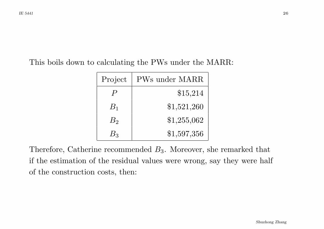
This boils down to calculating the PWs under the MARR:
Project PWs under MARR
P $15,214
B1 $1,521,260
B2 $1,255,062
B3 $1,597,356
Therefore, Catherine recommended B3. Moreover, she remarked that
if the estimation of the residual values were wrong, say they were half
of the construction costs, then:
Shuzhong Zhang
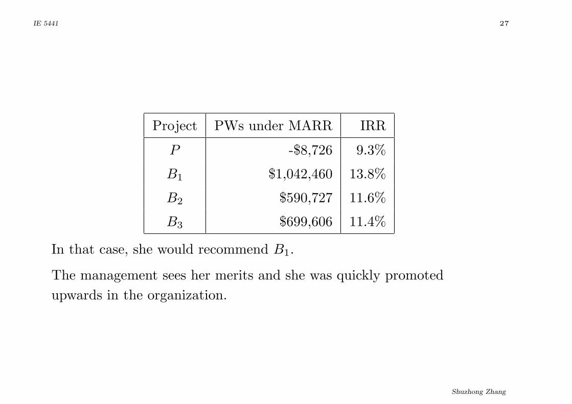
IE 5441 27
Project PWs under MARR IRR
P -$8,726 9.3%
B1 $1,042,460 13.8%
B2 $590,727 11.6%
B3 $699,606 11.4%
In that case, she would recommend B1.
The management sees her merits and she was quickly promoted
upwards in the organization.
Shuzhong Zhang
IE 5441 28
What to do when the duration (‘useful life’) of the projects are
different?
Obviously it is no longer “fair” only to compare the PWs. For
example, one project, P1, has a duration of 2 years, and the other
project, P2, has a duration of 4 years.
It can be that PWP1(MARR) < PWP2(MARR).
But, if we adopt P1 and replace the last two years with MARR, then
the combined project is more attractive than P2.
Shuzhong Zhang

IE 5441 29
We first consider the situation when a project can be repeated.
So we can try to fill up the whole time horizon with the same repeated
projects.
Let the duration of P1 be N1, and the duration of P2 be N2.
Let the least common multiple of N1 and N2 be N .
Let N = n1N1, and N = n2N2.
We then need to compare
PWn1P1(MARR) and PWn2P2
(MARR).
Shuzhong Zhang
IE 5441 30
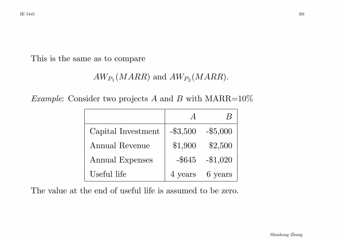
This is the same as to compare
AWP1(MARR) and AWP2(MARR).
Example: Consider two projects A and B with MARR=10%
A B
Capital Investment -$3,500 -$5,000
Annual Revenue $1,900 $2,500
Annual Expenses -$645 -$1,020
Useful life 4 years 6 years
The value at the end of useful life is assumed to be zero.
Shuzhong Zhang
IE 5441 31
Under the repeatability assumption, we need to compare 3A and 2B.
Or, equivalently, their Annual Worth: The AW of A is:
−$3, 500(A/P, 10%, 4) + $1, 900− $645 = $151
and the AW of B is:
−$5, 000(A/P, 10%, 6) + $2, 500− $1, 020 = $332.
Therefore, we prefer Project B.
However, not all projects can be repeated. Let us consider a more
general setting, when the study period is given.
That is, we are given: (1) the MARR; (2) the study period N ; (3) the
actual project. We want to evaluate whether or not the project is
more attractive than the MARR.
Shuzhong Zhang
IE 5441 32
General Approach:
Let the duration of Project P be Np. Suppose that the study period is
N .
Case 1. Np < N . There are two different possibilities: (A) P is a
service project; (B) P is an investment project.
In case of (A), one may consider repeating P till N is filled. Then
truncate the possible over-time.
In case of (B), one may re-invest the worth of P at the MARR till the
end.
Case 2. Np > N . Truncate the project at N using an estimated
market value of P at N .
Shuzhong Zhang
IE 5441 33
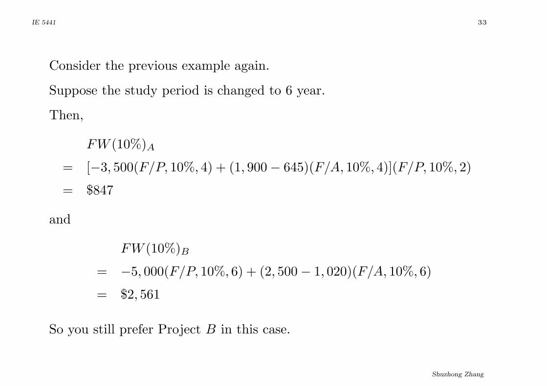
Consider the previous example again.
Suppose the study period is changed to 6 year.
Then,
FW (10%)A
= [−3, 500(F/P, 10%, 4) + (1, 900− 645)(F/A, 10%, 4)](F/P, 10%, 2)
= $847
and
FW (10%)B
= −5, 000(F/P, 10%, 6) + (2, 500− 1, 020)(F/A, 10%, 6)
= $2, 561
So you still prefer Project B in this case.
Shuzhong Zhang

IE 5441 34
Example: A company needs to have four additional forklift trucks to
support a warehouse, which is anticipated to be shutdown in 8 years.
Two mutually exclusive alternatives are identified:
Truck 1 Truck 2
Capital Investment -$184K -$242K
Annual Expense -$30K -$26.7K
Useful life 5 years 7 years
Salvage Value $17K $21K
The three-year lease cost is $104K per year.
The one-year lease cost is $134K per year.
The MARR of the firm is 15%.
Which type of the truck should the firm buy?
Shuzhong Zhang
IE 5441 35
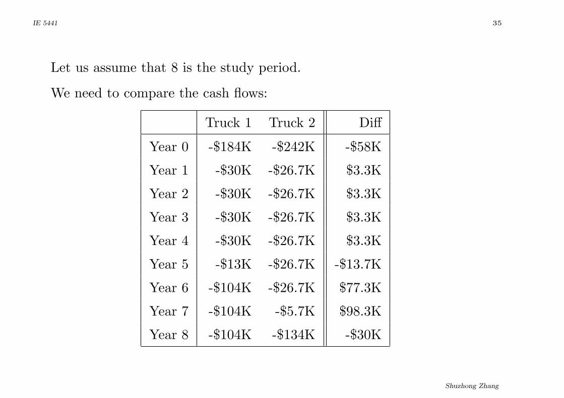
Let us assume that 8 is the study period.
We need to compare the cash flows:
Truck 1 Truck 2 Diff
Year 0 -$184K -$242K -$58K
Year 1 -$30K -$26.7K $3.3K
Year 2 -$30K -$26.7K $3.3K
Year 3 -$30K -$26.7K $3.3K
Year 4 -$30K -$26.7K $3.3K
Year 5 -$13K -$26.7K -$13.7K
Year 6 -$104K -$26.7K $77.3K
Year 7 -$104K -$5.7K $98.3K
Year 8 -$104K -$134K -$30K
Shuzhong Zhang
IE 5441 36
Since
PWDiff (15%) = $5, 171,
so we find Truck 2 more attractive.
One may also apply the ERR method to find
errDiff = 15.97%,
accepting the additional price for Truck 2.
Shuzhong Zhang

IE 5441 37
If the study period is shorter than the useful life of an equipment, then
it is crucial to estimate the market value of the equipment at that time.
The Imputed Market Value Technique:
(implied market value)
Suppose N < Np. Let MARR=r%, the initial capital investment be C
and the market value at Np be S. Then,
MVN = ‘Capital Recovery’× (P/A, r%, Np −N)
+S × (P/F, r%, Np −N).
In other words, MVN is the sum of two terms, the first being the PW
at year T of the remaining Capital Recovery value, and the second is
the PW at year T of the Salvage value.
Shuzhong Zhang
IE 5441 38
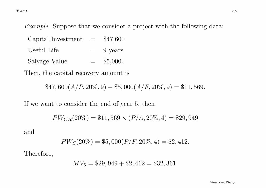
Example: Suppose that we consider a project with the following data:
Capital Investment = $47,600
Useful Life = 9 years
Salvage Value = $5,000.
Then, the capital recovery amount is
$47, 600(A/P, 20%, 9)− $5, 000(A/F, 20%, 9) = $11, 569.
If we want to consider the end of year 5, then
PWCR(20%) = $11, 569× (P/A, 20%, 4) = $29, 949
and
PWS(20%) = $5, 000(P/F, 20%, 4) = $2, 412.
Therefore,
MV5 = $29, 949 + $2, 412 = $32, 361.
Shuzhong Zhang
IE 5441 39
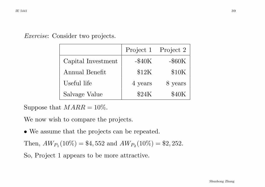
Exercise: Consider two projects.
Project 1 Project 2
Capital Investment -$40K -$60K
Annual Benefit $12K $10K
Useful life 4 years 8 years
Salvage Value $24K $40K
Suppose that MARR = 10%.
We now wish to compare the projects.
• We assume that the projects can be repeated.
Then, AWP1(10%) = $4, 552 and AWP2(10%) = $2, 252.
So, Project 1 appears to be more attractive.
Shuzhong Zhang
IE 5441 40
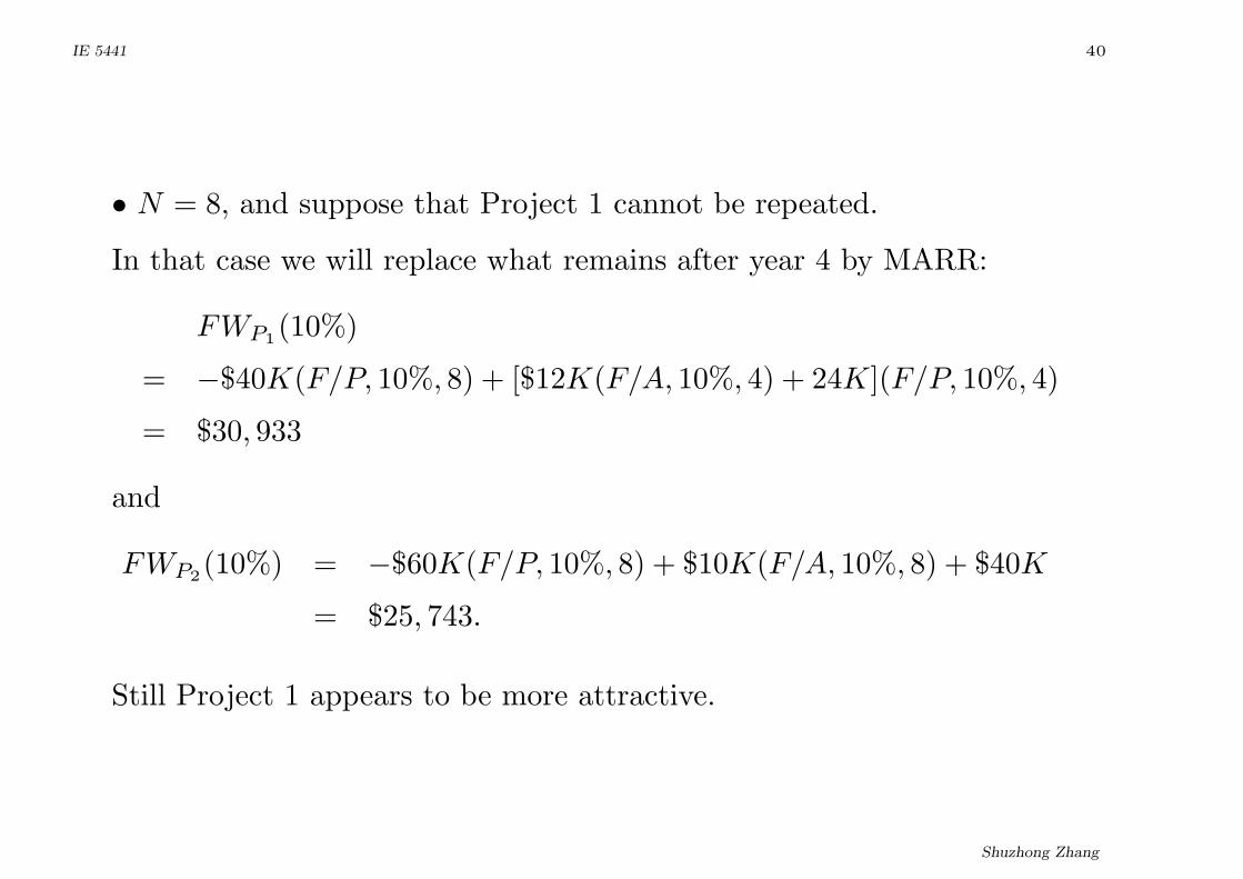
• N = 8, and suppose that Project 1 cannot be repeated.
In that case we will replace what remains after year 4 by MARR:
FWP1(10%)
= −$40K(F/P, 10%, 8) + [$12K(F/A, 10%, 4) + 24K](F/P, 10%, 4)
= $30, 933
and
FWP2(10%) = −$60K(F/P, 10%, 8) + $10K(F/A, 10%, 8) + $40K
= $25, 743.
Still Project 1 appears to be more attractive.
Shuzhong Zhang
IE 5441 41
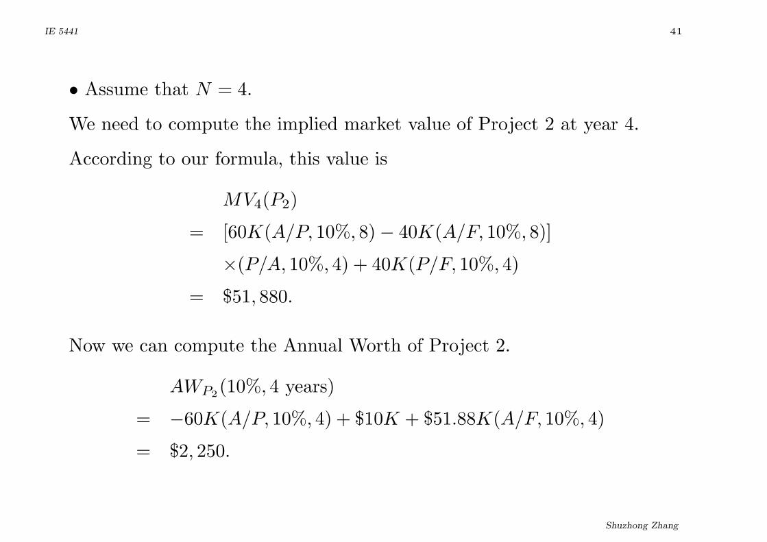
• Assume that N = 4.
We need to compute the implied market value of Project 2 at year 4.
According to our formula, this value is
MV4(P2)
= [60K(A/P, 10%, 8)− 40K(A/F, 10%, 8)]
×(P/A, 10%, 4) + 40K(P/F, 10%, 4)
= $51, 880.
Now we can compute the Annual Worth of Project 2.
AWP2(10%, 4 years)
= −60K(A/P, 10%, 4) + $10K + $51.88K(A/F, 10%, 4)
= $2, 250.
Shuzhong Zhang

IE 5441 42
What happens if the projects are not mutually exclusive?
This leads to the issue of capital budgeting:
maximize∑n
i=1 bixi
subject to∑n
i=1 cixi ≤ C
xi = 0 or 1, i = 1, ..., n.
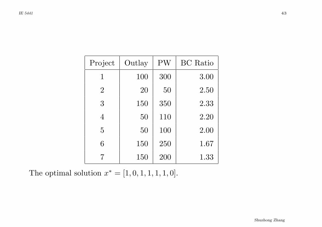
Example: Budgeting with a total budget of $500,000
Shuzhong Zhang
IE 5441 43
Project Outlay PW BC Ratio
1 100 300 3.00
2 20 50 2.50
3 150 350 2.33
4 50 110 2.20
5 50 100 2.00
6 150 250 1.67
7 150 200 1.33
The optimal solution x∗ = [1, 0, 1, 1, 1, 1, 0].
Shuzhong Zhang
IE 5441 44
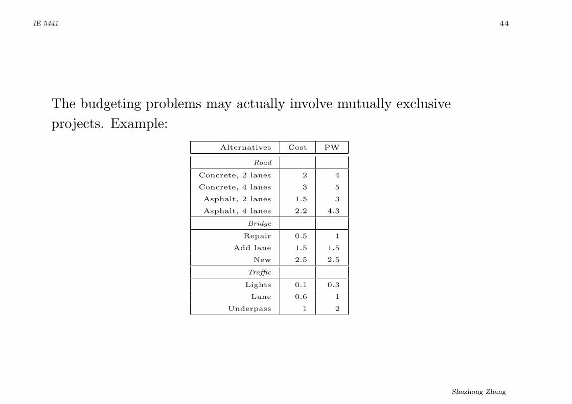
The budgeting problems may actually involve mutually exclusive
projects. Example:
Alternatives Cost PW
Road
Concrete, 2 lanes 2 4
Concrete, 4 lanes 3 5
Asphalt, 2 lanes 1.5 3
Asphalt, 4 lanes 2.2 4.3
Bridge
Repair 0.5 1
Add lane 1.5 1.5
New 2.5 2.5
Traffic
Lights 0.1 0.3
Lane 0.6 1
Underpass 1 2
Shuzhong Zhang
IE 5441 45
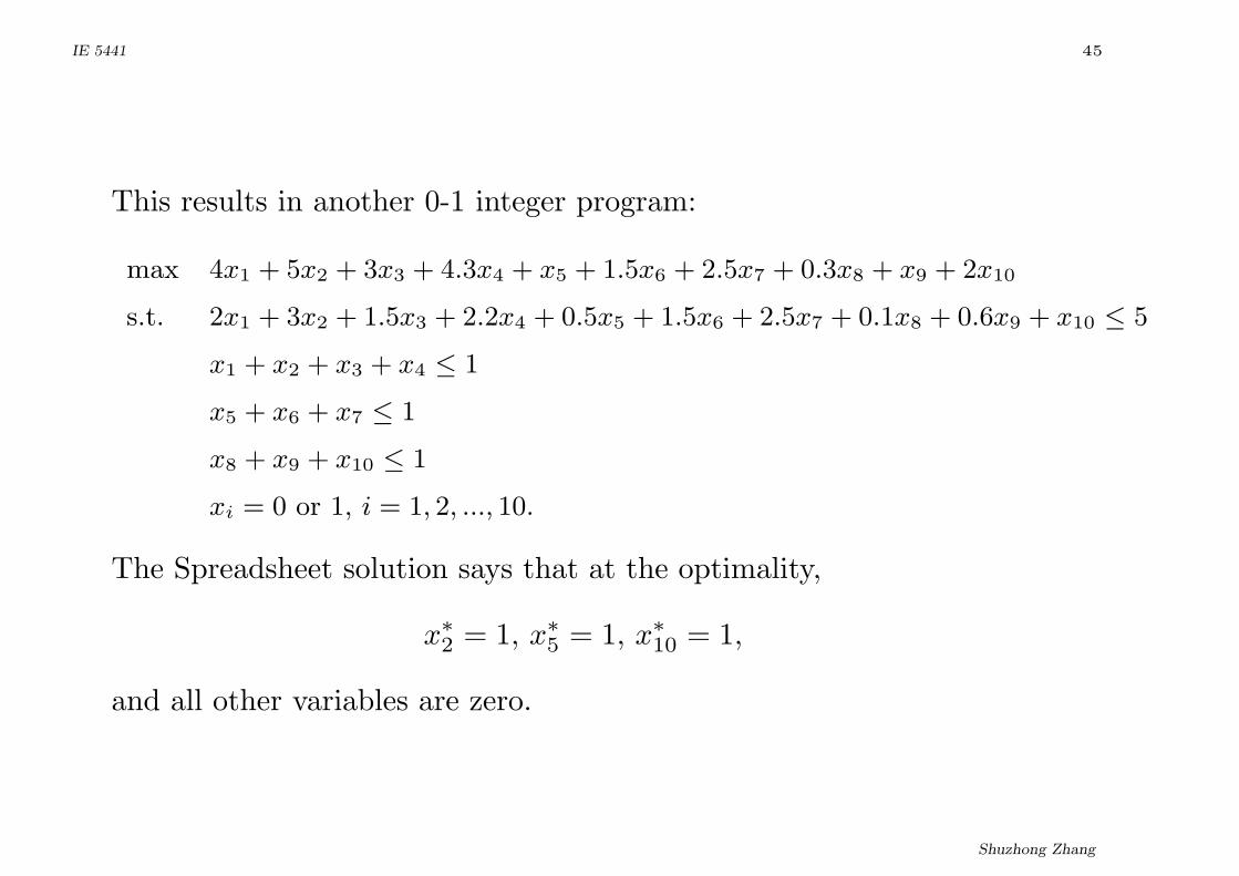
This results in another 0-1 integer program:
max 4x1 + 5x2 + 3x3 + 4.3x4 + x5 + 1.5x6 + 2.5x7 + 0.3x8 + x9 + 2x10
s.t. 2x1 + 3x2 + 1.5x3 + 2.2x4 + 0.5x5 + 1.5x6 + 2.5x7 + 0.1x8 + 0.6x9 + x10 ≤ 5
x1 + x2 + x3 + x4 ≤ 1
x5 + x6 + x7 ≤ 1
x8 + x9 + x10 ≤ 1
xi = 0 or 1, i = 1, 2, ..., 10.
The Spreadsheet solution says that at the optimality,
x∗2 = 1, x∗
5 = 1, x∗10 = 1,
and all other variables are zero.
Shuzhong Zhang
IE 5441 46
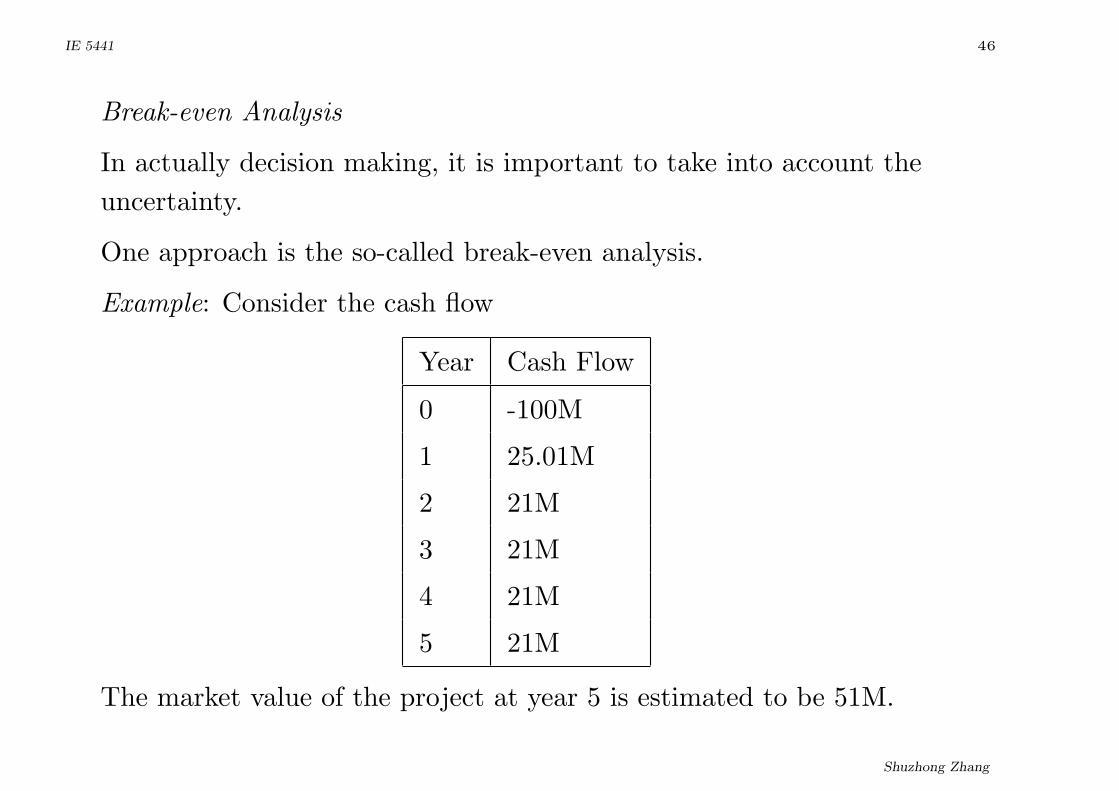
Break-even Analysis
In actually decision making, it is important to take into account the
uncertainty.
One approach is the so-called break-even analysis.
Example: Consider the cash flow
Year Cash Flow
0 -100M
1 25.01M
2 21M
3 21M
4 21M
5 21M
The market value of the project at year 5 is estimated to be 51M.
Shuzhong Zhang
IE 5441 47
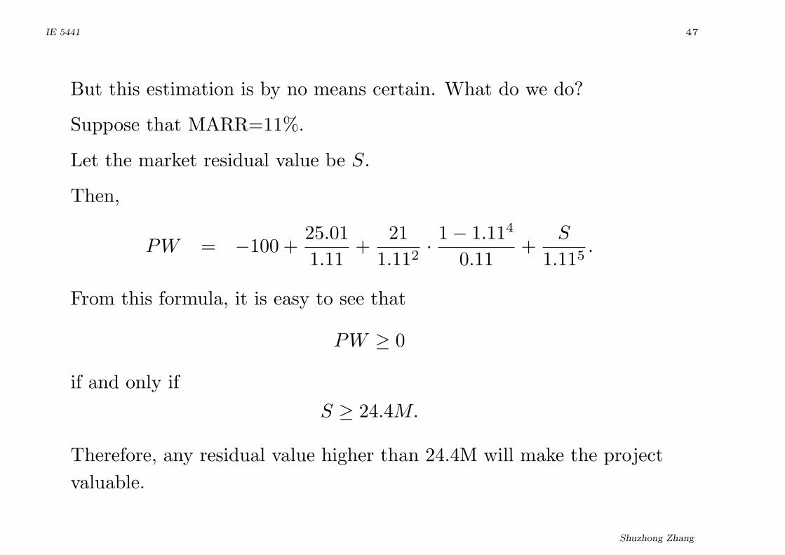
But this estimation is by no means certain. What do we do?
Suppose that MARR=11%.
Let the market residual value be S.
Then,
PW = −100 +25.01
1.11+
21
1.112· 1− 1.114
0.11+
S
1.115.
From this formula, it is easy to see that
PW ≥ 0
if and only if
S ≥ 24.4M.
Therefore, any residual value higher than 24.4M will make the project
valuable.
Shuzhong Zhang

IE 5441 48
Another example of this nature is as follows.
Consider the following project:
Investment -$1,000
Annual Return $400
Duration ?
MARR 10%
Let the duration be N . Then,
PW = −1, 000 + 4001− 1
1.1N
0.1.
Hence PW ≥ 0 if and only if
N ≥ 3.02 years.
Shuzhong Zhang
Recommended