Embed Size (px)
Citation preview

ZHAO FU
A STUDY OF STATIC STRAIN AGING OF SELECTED FERRITIC
STEELS
Master’s Thesis
Examiners: Associate Professor Pasi Peura and Doctoral Student Henri Järvinen The examiners and topic of thesis were approved on 31 May 2017

i
ABSTRACT
TAMPERE UNIVERSITY OF TECHNOLOGY Master’s Degree Program in Materials Engineering ZHAO FU: A Study of Static Strain Aging of Selected Ferritic Steels Master of Science Thesis, 85 pages, 11 Appendix pages May 2017 Major: Materials Science Examiners: Associate Professor Pasi Peura, Doctoral Student Henri Järvinen
Keywords: Low carbon steel, EN 1.4003 ferritic stainless steel, heat treatment, pre-strain, bake hardening, strain aging, yield strength, elongation
Bake hardening effect is a phenomenon of static strain aging and utilized in the
manufacturing of automotive components. Bake hardening occurs at elevated temperature
of around 170 °C during the paint-baking cycle of the formed components. It leads to the
strength increment by the diffusion of carbon atoms to the dislocations during the drying
of paint. Steels with ferritic microstructure are known to be susceptible to aging
phenomenon. In addition, low carbon steels and ferritic stainless steels are used to
produce certain automotive components. The aim of this work is to study the static strain
aging phenomenon of two low carbon steels and a ferritic stainless steel, more importantly,
by means of bake hardening tests.
This thesis consists of two parts, namely literature study and research parts. The literature
study covers the topics like carbon steel, ferritic stainless steel, strain aging, and bake
hardening. Two low carbon steels with small difference of production history and EN
1.4003 ferritic stainless steel were used for the experiments. Bake hardening (BH) tests,
consisting of pre-straining to 0%, 2%, 6%, and 10% and following heat-treatments of
170 °C/20min and 230 °C/20min, respectively, were conducted. The purpose of the heat
treatments was to simulate the paint baking process after press forming. In addition, to
evaluate the aging behavior during storage, a heat treatment of 100 °C/30 min (boiling
water) was carried out and was followed by tensile testing, respectively.
The study indicates that two low carbon steels have very similar initial properties and
behavior in the experiments. The 170 °C/20min heat treatment increased 41 MPa and
230 °C/20min increased around 130 MPa in yield strength of the low carbon steels, while
for EN 1.4003 ferritic stainless steel, these two numbers are 20 and 8 MPa, respectively.
The yield strength generally increased and elongation decreased with the increase of heat-
treatment temperature and pre-strain. The higher baking temperature led to greater BH
index generally. The BH index of low carbon steel increased from 19 MPa to around 54
MPa along with the pre-strain increasing from 0% to 10% when baked at 170°C, while it
decreased from 72 MPa to 58 MPa when baked at 230 °C. The 100 °C/30min aging
treatment did not produce significant influence on the properties of three investigated
ferritic steels. It can be concluded that the bake-hardening is the main mechanism of
achieving strength increase, and it heavily depends on the dislocation caused during pre-
strain.

ii
PREFACE
This thesis work was carried out at the Department of Materials Science of Tampere
University of Technology (Finland) between June 2016 and May 2017.
First of all, I would like to express my utmost gratitude to my thesis supervisor Associate
Professor Pasi Peura for offering this research project and giving constructive and helpful
advice on the thesis. Special gratitude is also given to M.sc. Henri Järvinen for his help
and helpful instruction in the experiments and results analysis throughout this thesis work.
Secondly, I would like to express my thanks to SSAB Europe Oy, Hämeenlinna and
Outokumpu Oyj for providing the materials for the experiments. At the meanwhile, I
would also thank FinDDRG ry (Finnish Deep Drawing Research Group) for granting the
thesis work.
Thirdly, Senior Laboratory Technician Ari Varttila conducted specimen machining work,
and few other laboratory technicians and researchers gave some help in the experiment, I
would also present my gratitude to them. My thanks is also given to the colleagues of our
research group and department for creating a friendly environment.
I would also express my thanks to my parents for their endless support and love, also, my
study in Finland would not be available without them. I am here also showing my greatest
gratitude to my home country China, which has always been in my mind and soul and
given me mental support.
In addition, my sincere gratitute is given to my wife Saara Pitkälä-Fu who has
accompanied me and given me lots of help, support and love. Last but not least, I also
express my thanks to some important friends in Finland Maarit Sulonen, Steven Kajiti,
Amad Ud Din Khattak, Anniina Vainionpää, who gave me lots of help in the life and
valuable friendship.
Zhao Fu
Tampere, 15.5.2017
iii
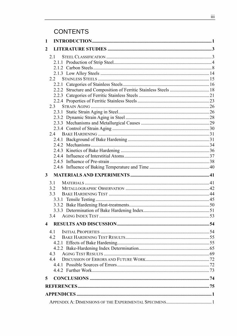
CONTENTS
1 INTRODUCTION .................................................................................................... 1
2 LITERATURE STUDIES ....................................................................................... 3
2.1 STEEL CLASSIFICATION ........................................................................................ 3
2.1.1 Production of Strip Steel.................................................................................. 4
2.1.2 Carbon Steels ................................................................................................... 8
2.1.3 Low Alloy Steels ........................................................................................... 14
2.2 STAINLESS STEELS ............................................................................................. 15
2.2.1 Categories of Stainless Steels ........................................................................ 16
2.2.2 Structure and Composition of Ferritic Stainless Steels ................................. 18
2.2.3 Categories of Ferritic Stainless Steels ........................................................... 21
2.2.4 Properties of Ferritic Stainless Steels ............................................................ 23
2.3 STRAIN AGING ................................................................................................... 26
2.3.1 Static Strain Aging in Steel ............................................................................ 26
2.3.2 Dynamic Strain Aging in Steel ...................................................................... 28
2.3.3 Mechanisms and Metallurgical Causes ......................................................... 29
2.3.4 Control of Strain Aging ................................................................................. 30
2.4 BAKE HARDENING ............................................................................................. 31
2.4.1 Background of Bake Hardening .................................................................... 31
2.4.2 Mechanisms ................................................................................................... 34
2.4.3 Kinetics of Bake Hardening .......................................................................... 36
2.4.4 Influence of Interstitial Atoms ....................................................................... 37
2.4.5 Influence of Pre-strain ................................................................................... 38
2.4.6 Influence of Baking Temperature and Time .................................................. 40
3 MATERIALS AND EXPERIMENTS .................................................................. 41
3.1 MATERIALS ........................................................................................................ 41
3.2 METALLOGRAPHIC OBSERVATION ...................................................................... 42
3.3 BAKE HARDENING TEST .................................................................................... 44
3.3.1 Tensile Testing ............................................................................................... 45
3.3.2 Bake Hardening Heat-treatments ................................................................... 50
3.3.3 Determination of Bake Hardening Index....................................................... 51
3.4 AGING INDEX TEST ............................................................................................ 53
4 RESULTS AND DISCUSSION ............................................................................. 54
4.1 INITIAL PROPERTIES ........................................................................................... 54
4.2 BAKE HARDENING TEST RESULTS ...................................................................... 55
4.2.1 Effects of Bake Hardening............................................................................. 55
4.2.2 Bake-Hardening Index Determination ........................................................... 65
4.3 AGING TEST RESULTS ........................................................................................ 69
4.4 DISCUSSION OF ERRORS AND FUTURE WORK ..................................................... 72
4.4.1 Possible Sources of Errors ............................................................................. 72
4.4.2 Further Work .................................................................................................. 73
5 CONCLUSIONS .................................................................................................... 74
REFERENCES .............................................................................................................. 75
APPENDICES ................................................................................................................. 1
APPENDIX A: DIMENSIONS OF THE EXPERIMENTAL SPECIMENS ...................................... 1

iv
APPENDIX B: REPRESENTATIVE ENGINEERING STRESS-STRAIN CURVES FOR MATERIALS
TESTED IN INITIAL CONDITION AND AFTER BAKE HARDENING HEAT TREATMENTS, NO
PRE-STRAIN .................................................................................................................... 2
APPENDIX C: REPRESENTATIVE ENGINEERING STRESS-STRAIN CURVES DESCRIBING THE
EFFECTS OF PRE-STRAINING AND BAKE HARDENING HEAT TREATMENTS ...................... 4
APPENDIX D: BAKE HARDENING INDEXES OF INVESTIGATED STEELS ............................ 7
APPENDIX E: REPRESENTATIVE ENGINEERING STRESS-STRAIN CURVES OF THE
SPECIMENS BEFORE AND AFTER AGING TREATMENT ..................................................... 9

v
LIST OF FIGURES
Figure 1. Iron-carbon phase diagram [6]. ......................................................................... 3
Figure 2. Diagram of an electric arc furnace with direct current [11]. ............................ 4
Figure 3. Illustration of blast furnace process [12]. ......................................................... 5
Figure 4. Schematic of steelmaking process with basic oxygen furnace [14]. ................ 5
Figure 5. Schematic of curved continuous casting process [16]. ..................................... 6
Figure 6. Schematic of annealing cycles for batch and continuous annealing [7]. .......... 7
Figure 7. Variations of mechanical properties of as-rolled 25 mm daim bars of
plain carbon steels as a function of carbon content [22]. ........................ 10
Figure 8. Micrographs of (a) low carbon AISI/SAE 1010 steel; (b) medium
carbon AISI/SAE 1040 steel; (c) high carbon AISI/SAE 1095 steel
[5]. ........................................................................................................... 11
Figure 9. Micrographs of (a) upper bainite and (b) lower bainite with intra-lath
carbide segregation; (c) SEM image of upper bainite; (d) Acicular
ferrite [29]. ............................................................................................... 13
Figure 10. Micrograph of a high strength low alloyed linepipe steel [5]. ...................... 15
Figure 11. Chromium contents of different categories of stainless steels [41]. ............. 16
Figure 12. Impact toughness of different types of stainless steels [40]. ........................ 17
Figure 13. Micrographs of ferritic stainless steel: (a) AISI 409; (b) AISI 439 [43]. ..... 18
Figure 14. Phase diagram of Fe-Cr alloy system [44].................................................... 18
Figure 15. Schaffer diagram of stainless steels [46]. ..................................................... 19
Figure 16. Micrographs of the 𝛿 → 𝜎 + 𝛾2 transformation in AISI 304 stainless
steel (650°C, 31000 h) [49]. .................................................................... 20
Figure 17. Diagram of hardness as a function of time of few ferritic stainless
steels during the formation of α’ phase [47]. ........................................... 20
Figure 18. Effects of carbon content on mechanical properties of 13% Cr stainless
after quenching and after relieving with 200°C heat treatment [46]. ...... 22
Figure 19. Comparison of stress-strain behavior of austenitic, duplex, ferritic
stainless steels and carbon steel [53]. ...................................................... 24
Figure 20. Schematic representation of the influence of strain aging on the stress-
strain curve for low carbon steel [59]. ..................................................... 27
Figure 21. Load-elongation curve of a low-carbon steel with Lüders bands [60]. ........ 27
Figure 22. True flow stress – temperature relations of low carbon steel showing
anomalous strain rate effect due to dynamic strain aging [63]. ............... 28
Figure 23. Schematic representation of strength-elongation combination of
different types of steels used in the parts of cars [78]. ............................ 32
Figure 24. Schematic illustration of the behavior of bake hardening steel
compared with mild IF steel and rephosphorised steel [79]. ................... 33
Figure 25. Schematic representation of bake hardening response in tensile test
[80]. ......................................................................................................... 33
Figure 26. Schematic illustration of three stages in bake hardening [90]. ..................... 35

vi
Figure 27. Diagram of engineering stress-strain curve of low carbon steel
demonstrating the variation of dislocation and carbon atoms [91]. ........ 35
Figure 28. Schematic presentation of the yield strength as a function of ageing
time during bake hardening process [80]. ............................................... 36
Figure 29. Yield strength increment as a function of free carbon content during
bake hardening response [79]. ................................................................. 38
Figure 30. Yield strength increment as a function of carbon content in solution
during bake hardening response [94]. ..................................................... 38
Figure 31. Increase of yield strength of ultralow carbon steel with different pre-
strains of 1%, 2%, 5%, and 10%, respectively [83]. ............................... 39
Figure 32. Optical micrographs of the investigated steels: (a) A material of
longitudinal direction, (b) A material of transverse direction, (c) B
material of longitudinal direction, (d) B material of transverse
direction, (e) C material (EN 1.4003 ferritic stainless steel) of
transverse direction. ................................................................................. 43
Figure 33. Illustration of the method of measuring grain sizes of initial materials. ...... 44
Figure 34. Example specimen showing the necking at softer areas in pre-strained
and baked condition. The specimen was re-machined after pre-
straining in order to avoid the observed phenomenon............................. 46
Figure 35. Instron 8801 hydraulic testing machine [99]. ............................................... 46
Figure 36. Schematic of strain measurement with clip-on extensometer [100]. ............ 47
Figure 37. Diagram of 0.2% offset yield strength determination with engineering
strain-stress curve without sharp yield point. .......................................... 49
Figure 38. Schematic diagram of tensile test piece in which the fractures are not
in the ideal gauge section. ....................................................................... 50
Figure 39. Example of engineering stress-strain curve of the discontinuous
yielding specimens in the tests. ............................................................... 50
Figure 40. Schematic presentation of heat treatment procedures in the
experiments.............................................................................................. 51
Figure 41. Schematic illustration of bake-hardening index BH2 determination
method applied for low carbon steels. ..................................................... 52
Figure 42. Schematic illustration of bake-hardening index BH2 determination
method applied for ferritic stainless steels. ............................................. 52
Figure 43. Schematic diagram of aging treatment technology in the experiments. ....... 53
Figure 44. Illustration of yield strength value determination methods with
different engineering stress-strain curves. ............................................... 56
Figure 45. Yield strength (determined with higher yield point) of steels A and B
at initial status and after different pre-straining and bake hardening
treatments. ............................................................................................... 57
Figure 46. Yield strength (determined with lower yield point) of steels A and B at
initial status and after different pre-straining and bake hardening
treatments. ............................................................................................... 58

vii
Figure 47. Lüders bands at 45° from the tensile axis [101]. .......................................... 59
Figure 48. Total elongation of steels A and B at initial status and after different
pre-straining and bake hardening treatments. .......................................... 60
Figure 49. Mechanical properties of steel C at initial status and after different pre-
straining and 170 °C/20min bake hardening treatment. .......................... 61
Figure 50. Mechanical properties of steel C at initial status and after different pre-
straining and 230 °C/20min bake hardening treatment. .......................... 62
Figure 51. Illustration of the bake-hardening indexes determination. Tensile test
specimens: B9 (2% pre-strain and 230 °C/20min), B13 (6% pre-
strain and 230 °C/20min), B17 (10% pre-strain and 230 °C/20min). ..... 63
Figure 52. Illustration of bake-hardening response and work-hardening response
in the engineering stress-strain curve. ..................................................... 64
Figure 53. Bake-hardening indexes for steel A with two bake-hardening heat
treatments. ............................................................................................... 66
Figure 54. Bake-hardening indexes for steel B with two bake-hardening heat
treatments. ............................................................................................... 66
Figure 55. Bake-hardening indexes for steel C with two bake-hardening heat
treatments. ............................................................................................... 67
Figure 56. Mechanical properties of steel A before and after 100 °C/30 min aging
treatment. ................................................................................................. 70
Figure 57. Mechanical properties of steel B before and after 100 °C/30 min aging
treatment. ................................................................................................. 70
Figure 58. Mechanical properties of steel C (1.4003 ferritic stainless steel) before
and after 100 °C/30 min aging treatment. ............................................... 71
viii
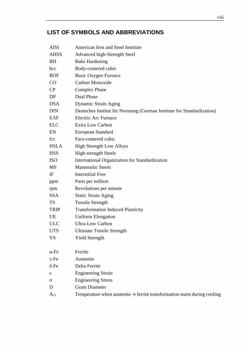
LIST OF SYMBOLS AND ABBREVIATIONS
AISI American Iron and Steel Institute
AHSS Advanced high-Strength Steel
BH Bake Hardening
bcc Body-centered cubic
BOF Basic Oxygen Furnace
CO Carbon Monoxide
CP Complex Phase
DP Dual Phase
DSA Dynamic Strain Aging
DIN Deutsches Institut für Normung (German Institute for Standardization)
EAF Electric Arc Furnace
ELC Extra Low Carbon
EN European Standard
fcc Face-centered cubic
HSLA High Strength Low Alloys
HSS High-strength Steels
ISO International Organization for Standardization
MS Martensitic Steels
IF Interstitial Free
ppm Parts per million
rpm Revolutions per minute
SSA Static Strain Aging
TS Tensile Strength
TRIP Transformation Induced Plasticity
UE Uniform Elongation
ULC Ultra-Low Carbon
UTS Ultimate Tensile Strength
YS Yield Strength
α-Fe Ferrite
γ-Fe
Austenite
δ-Fe Delta Ferrite
ε Engineering Strain
σ Engineering Stress
D Grain Diameter
Ar3 Temperature when austenite → ferrite transformation starts during cooling

1
1 INTRODUCTION
Vehicle shows an increasing significance in the society and our daily life. Low and
medium carbon steels (carbon content up to 0.35) are the most widely used materials in
the automotive manufacturing. In addition, ferritic stainless steels are also used in some
automotive parts. However, they have not reached that much attention with respect to the
typical phenomena occurring in the manufacturing routines. Therefore, the pre-straining,
bake-hardening (BH) heat treatments, tensile tests, aging treatments were performed to
study the static strain aging phenomenon by investigating the bake hardening response.
Static strain aging (SSA) is a general phenomenon in steels typically utilized in bake
hardening and multi-phase steels. Bake hardening, in turn, is a phenomenon of SSA,
which leads to the strength increment because of the work hardening in the cold working
and the strain aging during the subsequent paint baking during manufacturing of
automotive components [1]. Low carbon steels are known to be sensitive to SSA behavior,
i.e., they show bake hardening when they are subjected to forming and subsequent paint
baking during manufacturing of automotive components. For example, Banerjee and Dhal
[2] confirmed the strain aging response of low carbon steel. However, the bake hardening
behavior of ferritic stainless steels has not reached that much attention even though they
are also used in some automotive parts.
But there exists some studies [3-4], which have shown that SSA can also occur in ferritic
stainless steels. For example, Palosaari, et al. [3] also found that a strength increment of
50 MPa with EN 1.4509 and 1.4521 ferritic stainless steels due to the strain aging. Buono,
et al. [4] found that the yield strength of AISI 430 stainless steel increased from 465 MPa
to 528 MPa with the increase of baking temperature from 180 °C to 245 °C, with a 30
min bake-hardening time. However, the information on the static strain aging of
unstabilized ferritic stainless steels is still limited.
Therefore, this research aims at gaining a further understanding of the impact of the static
strain aging phenomenon on the mechanical properties, it also studies the behavior of the
low carbon steels and EN 1.4003 ferritic stainless steels in the automotive components
manufacturing by investigating the response of its mechanical properties. The research is
expected to understand how the pre-strain and heat treatment affect the mechanical

2
properties and how much strength can be increased by the strain aging phenomenon.
Chapter 2 includes some relevant theoretical information, which includes the topics of
carbon steel, alloy steel, ferritic stainless steel, strain aging, and bake hardening. Chapter
3 describes the experimental materials and methods, the results are presented and
analyzed, some problems and future work in the relevant field are also discussed in
Chapter 4. Some significant findings are presented in Chapter 5. Some appendices are
also attached in the end of the thesis to provide more detailed information on how the
data were produced.

3
2 LITERATURE STUDIES
2.1 Steel Classification
Steel is a hard and strong iron-based alloy. It is one of the most widely used materials in
the current life around the world, especially in the engineering and construction fields.
The Carbon content is mostly no more than 2.11%, as shown in Figure 1. It is the most
important element for iron and for the properties of steels, the carbon content also affects
the hardness, tensile strength, ductility of the steel a lot [5].
The microstructures and properties of the steels are significantly influenced by their
composition, therefore, the chemical composition is commonly used as criterion to
classify the steels. By chemical composition, the steel can be classified into carbon steels
and alloy steels, the difference of which is that in the carbon steel, carbon is the main
element, while alloy steels contain more alloying elements for improving some properties.
Figure 1. Iron-carbon phase diagram [6].

4
2.1.1 Production of Strip Steel
The development of steel making technologies and the application of vacuum degassing
make it easy to control the contents of some elements like carbon, nitrogen, sulphur, etc.
Before 1970s, the main parts of the strip steel was casted into ingots with 500 mm
thickness, and then be cooled and removed from modules, which is followed by heating
to around 1250°C and rolling to slabs with 200-250 mm thickness and cooling [7]. The
surface defects were finally removed through scarfing. The different stages of this process
were separated [7]. Steel is normally manufactured from two kinds of raw materials: steel
scrap and hot metals. Steel scrap is normally produced by using electric arc furnace (EAF),
and hot metal is typically produced by blast furnace.
Since the EAF for steelmaking in 1889 by Paul Héroult, EAF has been widely applied in
steelmaking and smelting of nonferrous metals, including stainless steel [8]. EAF is also
the core process of mini-mills, which produce steel from scrap [9]. An EAF melts
minerals or other materials by using electricity. The dry minerals are firstly weighed and
mixed, which are then evenly distributed throughout the furnace. Power is supplied
through a transformer and graphite electrodes, the electrodes are extended into the furnace
and touch the materials, and the electric arc can be formed between the electrodes when
power is supplied, as indicated in Figure 2. The electric arc melts the materials and
produce a liquid bath [10]. The temperature in EAF is very high depending on the melting
point of the metal. There is also a water cooling system to avoid overheating. The melted
liquid material is then poured into a mold and sent to the cooling system, the ingot would
be solidified and processed to the desired size and shape [10].
Figure 2. Diagram of an electric arc furnace with direct current [11].
5
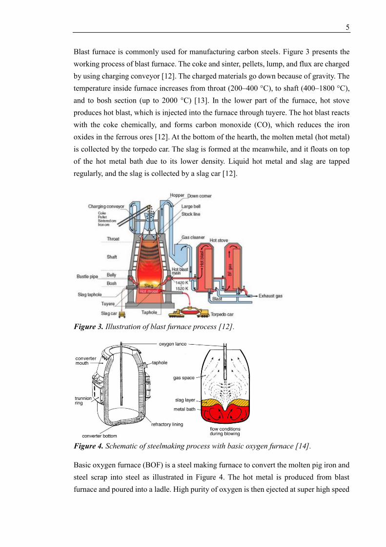
Blast furnace is commonly used for manufacturing carbon steels. Figure 3 presents the
working process of blast furnace. The coke and sinter, pellets, lump, and flux are charged
by using charging conveyor [12]. The charged materials go down because of gravity. The
temperature inside furnace increases from throat (200–400 °C), to shaft (400–1800 °C),
and to bosh section (up to 2000 °C) [13]. In the lower part of the furnace, hot stove
produces hot blast, which is injected into the furnace through tuyere. The hot blast reacts
with the coke chemically, and forms carbon monoxide (CO), which reduces the iron
oxides in the ferrous ores [12]. At the bottom of the hearth, the molten metal (hot metal)
is collected by the torpedo car. The slag is formed at the meanwhile, and it floats on top
of the hot metal bath due to its lower density. Liquid hot metal and slag are tapped
regularly, and the slag is collected by a slag car [12].
Figure 3. Illustration of blast furnace process [12].
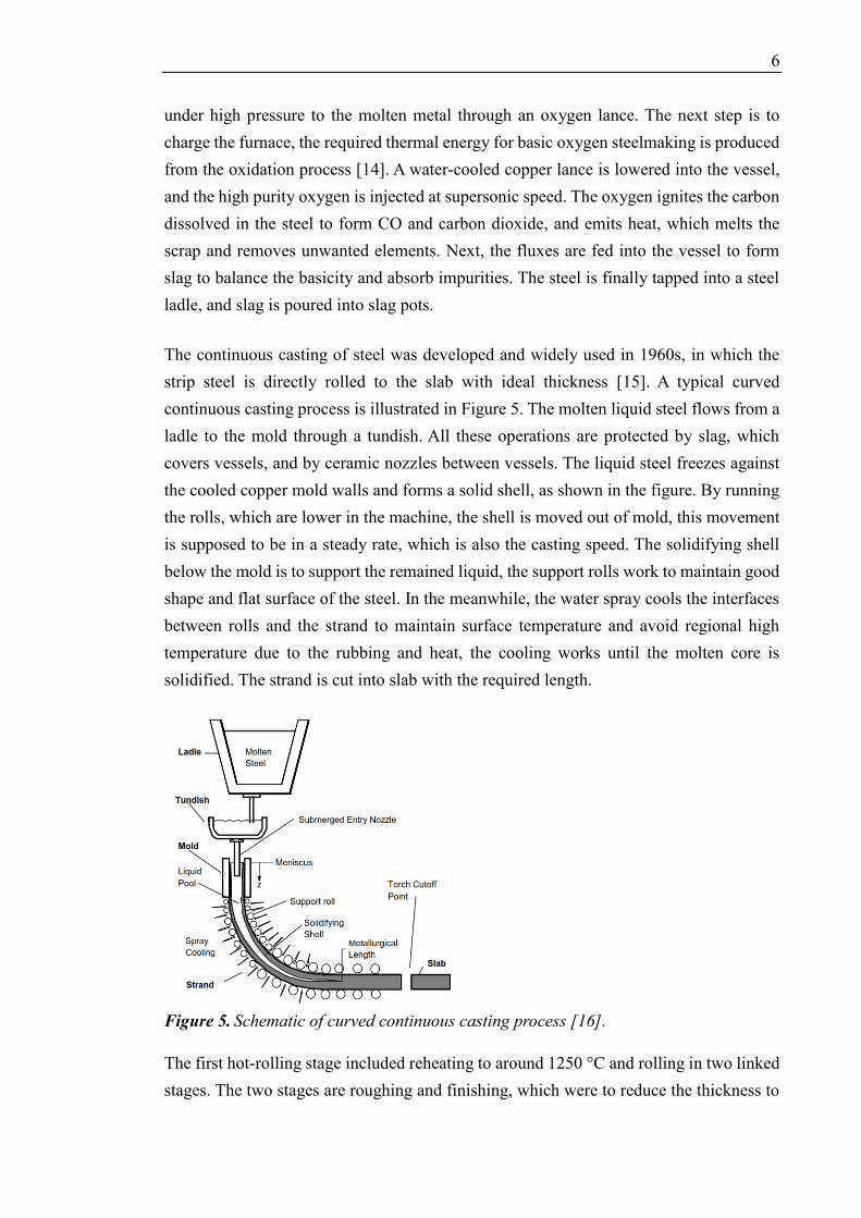
Figure 4. Schematic of steelmaking process with basic oxygen furnace [14].
Basic oxygen furnace (BOF) is a steel making furnace to convert the molten pig iron and
steel scrap into steel as illustrated in Figure 4. The hot metal is produced from blast
furnace and poured into a ladle. High purity of oxygen is then ejected at super high speed
6
under high pressure to the molten metal through an oxygen lance. The next step is to
charge the furnace, the required thermal energy for basic oxygen steelmaking is produced
from the oxidation process [14]. A water-cooled copper lance is lowered into the vessel,
and the high purity oxygen is injected at supersonic speed. The oxygen ignites the carbon
dissolved in the steel to form CO and carbon dioxide, and emits heat, which melts the
scrap and removes unwanted elements. Next, the fluxes are fed into the vessel to form
slag to balance the basicity and absorb impurities. The steel is finally tapped into a steel
ladle, and slag is poured into slag pots.
The continuous casting of steel was developed and widely used in 1960s, in which the
strip steel is directly rolled to the slab with ideal thickness [15]. A typical curved
continuous casting process is illustrated in Figure 5. The molten liquid steel flows from a
ladle to the mold through a tundish. All these operations are protected by slag, which
covers vessels, and by ceramic nozzles between vessels. The liquid steel freezes against
the cooled copper mold walls and forms a solid shell, as shown in the figure. By running
the rolls, which are lower in the machine, the shell is moved out of mold, this movement
is supposed to be in a steady rate, which is also the casting speed. The solidifying shell
below the mold is to support the remained liquid, the support rolls work to maintain good
shape and flat surface of the steel. In the meanwhile, the water spray cools the interfaces
between rolls and the strand to maintain surface temperature and avoid regional high
temperature due to the rubbing and heat, the cooling works until the molten core is
solidified. The strand is cut into slab with the required length.
Figure 5. Schematic of curved continuous casting process [16].
The first hot-rolling stage included reheating to around 1250 °C and rolling in two linked
stages. The two stages are roughing and finishing, which were to reduce the thickness to

7
30-45 mm, and reduced to 1-12 mm depending on the mill and final hot-rolled gauge
requirement [7]. The roughing could be performed with a single reversing stand, through
which the steel passes forwards and backwards several times. The finishing is performed
with a finishing train which contains normally seven stands. The front end of the strip
exists the last stand well before the back end of the strip enters the first stand. The
finishing temperature when the steel comes to the last stand is supposed to be over Ar3
temperature, which is to ensure the constituent transformation happens in the austenite
region of the phase diagram, as indicated in Figure. 1. The steel is then cooled before
coiling, the temperature of which ranges from 200 °C to 750 °C depending on the
metallurgic issues. If needed, the steel is then passed through a pickling line together with
hydrochloric acid to remove the oxide on the surface [17].
The cold rolling is carried out by a tandem mill containing typically five stands. Cold
rolling makes steel stronger, harder, but more brittle. To reduce the strength and improve
the formability, the cold rolled steel usually needs to be annealed. The recrystallization,
grain formation and growth, precipitates dissolution happen during the annealing. The
interaction of these changes determines the final microstructures and properties of the
steel [7]. Batch annealing and continuous annealing are the common methods. Batch
annealing is performed in a furnace, the steel is enclosed in it with the protective
atmosphere, which has been NHX gas (nitrogen with no more than 5% hydrogen) or pure
hydrogen. Pure hydrogen is more preferred for its faster heat transfer, which causes rapid
heating and cooling [18]. In continuous annealing, the annealing time is much shorter
than in batch annealing, as indicated in Figure 6. The batch annealing temperature can be
up to 700 °C for most cases, whereas continuous annealing temperature for strip steels is
above 700 °C and often above 800 °C [7, 19].
Figure 6. Schematic of annealing cycles for batch and continuous annealing [7].
The last stage in steel processing is the temper rolling or skin passing, which is to remove
the yield point in the tensile curve to avoid the occurrence of the stretcher-strain markings
while the steel is being pressed. The metallic coating with electrolytic process can all be
achieved by hot dipping and be applied to the annealed strip surface. [7]

8
2.1.2 Carbon Steels
By the definition of American Iron and Steel Institute (AISI), carbon steel has no specific
content for chromium, nickel, molybdenum, cobalt, tungsten, etc., nor requirements for
other elements for obtaining desired properties. Carbon is the main alloying element for
steel, the content of carbon can reach 2% in steels. It is usually dissolved in the iron or be
present as carbide Fe3C. The Increase of carbon content can increase the hardness, tensile
strength, solid-solution strength, hardenability while reduce the weldability [5, 20].
Carbon steel usually contains up to 1.4% manganese, which prevents the formation of
iron sulfide inclusions FeS, which has low melting point and is formed at grain boundaries
mostly [20].
Manganese content normally ranges from 0.2% in the steel, in the carbon steel, it is
common to reach 1.5% [20]. It also contributes to the increase of solid-solution strength,
hardness and hardenability, to be more precise, manganese increases the strength of ferrite.
It can also combine with sulphur to form globular manganese sulphides (MnS), which
improves machinability. At the same time, it counters the brittleness from sulphur, which
is good for the surface finish of the carbon steel [5].
Silicon strengthens the iron by dissolving into it. It also inhibits the grain growth by
limiting the prior austenite size. Meanwhile, the addition of silicon increases the ultimate
tensile strength and decreases yield stress [21]. It is also a principal deoxidizer in the steel
to remove oxygen, and form silicate stringers (silicon dioxide inclusions) [5].
Aluminum contributes to the deoxidization of the steel by extracting gases from the steel,
and it also offers the resistance to aging. It increases the hardness and toughness of the
steel by combining with nitrogen to form very hard nitride and forming fine grain
microstructures. In addition, aluminum does not form carbide either [5].
Chromium increases the hardenability and corrosion resistance of the carbon steel. Sulfur
is usually undesirable impurity in the steels, the amount of which is normally strictly
limited. When its content is above 0.05%, brittleness may be caused and weldability can
be decreased [20]. Similarly, phosphorus is also undesirable impurity, the amount of
which is normally strictly limited in the carbon steels, otherwise, it may bring
embrittlement in the hardened steels [20]. Molybdenum promotes the carbide formation
very well, and increases the hardenability and strength. It is usually in small amount of
no more than 0.2% in the carbon steel. Nickel increases the hardenability, toughness and
ductility, especially when at low temperature for the carbon steel, and its content is usually

9
below 0.5% [20]. Vanadium and niobium both increase the hardenability of carbon steel,
and they are present in small amount of lower than 0.2% and 0.02%, respectively [20].
The main elements and their functions in the steel are summarized in Table 1.
Table 1. Main elements in the steels and their functions [5].
Elements Functions
Carbon The most fundamental element in the steels. It increases the hardness
and strength generally. It can also form cementite Fe3C with iron.
Manganese Increases the solid-solution hardness and hardenability. It lowers the
hot brittleness, but high content of manganese produces austenitic
microstructure and makes the steel brittle.
Silicon Increases the solid-solution hardness, strength and hardenability. Also
removes oxygen in the molten steels. It increases the oxidation
resistance, and susceptibility to decarburization.
Aluminum It contributes to the deoxidization of the steel and it offers resistance to
aging. It forms small grains to improve the hardness and toughness.
Nickel Increases the solid-solution hardness, strength, toughness and
hardenability of the steels.
Chromium Slightly increase the solid-solution hardness, toughness and
hardenability of the steels. Increases the corrosion resistance at high
temperature. It forms the carbides, which improves the wear resistance.
Molybdenum Strong carbide former, which improves the creep strength, hardness. It
also improves the corrosion resistance in the stainless steels.
Cobalt Increases hardness at high temperature and the strength of the steels. It
is weak carbide former. It decreases the hardenability.
Titanium It refines the grains to increase the strength and hardness of the steels.
It is very strong carbide former, good to combine with nitrogen. It is
also strong oxidizer.
Phosphorus It is impurity in the steel. It improves the machinability and increases
the hardness and strength of low-carbon steels.
The mechanical properties of carbon steels are established and affected by the material
specifications, the property values can vary within certain range with different material
specifications [18]. The properties of the carbon steel cover a wide range, which is
affected by the composition a lot. Among all the elements, the content of carbon has a
critical impact on the mechanical properties, which is demonstrated in Figure 7. It can be
seen that the hardness, tensile strength, yield strength (YS), reduction, and elongation are
all affected significantly by the variation of carbon content.

10
Figure 7. Variations of mechanical properties of as-rolled 25 mm daim bars of plain
carbon steels as a function of carbon content [22].
By the carbon content, carbon steel can be classified into low-carbon steels, medium-
carbon steels, high-carbon steels, ultrahigh-carbon steels, the carbon contents of which
range between 0-0.30%, 0.30%-0.60%, 0.60%-1.00%, and 1.25%-2.00%, respectively [7].
With the increase of carbon content, the hardness and tensile strength, and toughness are
increased, while brittleness is decreased.
Low carbon steels contain no more than 0.3% carbon. They are mostly applied to
manufacture the flat-rolled products, e.g. strip or sheet, under cold-rolled and annealed
condition. When the carbon content is below 0.1%, the carbon steel has good formability,
which makes it ideal material for the automobile body panels and wire products. When
the content is up to 0.3% with manganese content up to 0.4%, it is good for rolled steel
structural plates. While when the manganese content reaches 1.5%, the carbon steel is
ideal material for forgings, seamless tubes, and boiler plates [22].
Medium-carbon steels contain 0.30% to 0.60% carbon and 0.60% to 1.65% manganese
[22]. They have good thermal processing property and poor weldability. Due to the higher
carbon content, their hardness and strength are higher, brittleness and toughness are lower
than in low-carbon steels. Medium-carbon steels are mostly applied for gears, crankshafts,
axles, forgings, and etc. They can be applied under the quenched and tempered condition
when the carbon content reaches 0.5% [22].

11
High-carbon steels contain 0.60% to 1.00% carbon and 0.30% to 0.90% manganese [22].
They have fully pearlitic microstructure, which is very fine structure and makes the steel
very hard, while less ductile than medium-carbon steels [23]. The strength and hardness
are further higher, brittleness and toughness are lower than the medium-carbon steels due
to the increase of the carbon content. They are often applied for springs and high-strength
steel wires [22-23]. They are also called tool steels since they are well used as the material
for some tools like saw blades, knives, chains, shear blades, etc. [23-24].
Ultrahigh-carbon steels contain 1.25% to 2.00% carbon [25]. As indicated in Figure 1, its
microstructure is cementite and pearlite at low temperature (below 1000 K), with the
increase of temperature, austenite would occur and the portion of cementite would be
decreased. The further increase of temperature would increase the portion of austenite
and ferrite is also possible to occur. Therefore, they usually have very high hardness and
strength, which makes them ideal materials for some knives, molds and other tools.
Figure 8. Micrographs of (a) low carbon AISI/SAE 1010 steel; (b) medium carbon
AISI/SAE 1040 steel; (c) high carbon AISI/SAE 1095 steel [5].

12
The difference of compositions also influences the microstructures of the steels. Low-
carbon steel consists mainly ferrite grains, which is the white etching part in Figure 8(a),
and pearlite, which is the dark etching part shown in Figure 8(a). The ferrite grains and
pearlite in the medium-carbon steels is shown in Figure 8(b) with white etching and dark
etching parts, respectively. In high-carbon steels, there are mainly pearlite matrix and
grain-boundary cementite, which is shown in Figure 8(c).
Low-carbon steel consists of mainly ferrite, as indicated in Figure 1, for example, a steel
with 0.4% C consists of single phase austenite (γ-Fe), with cooling slowly, some austenite
transform to ferrite (α-Fe) when the temperature is above 727 °C. When it is cooled to
below 727 °C, the remained austenite transform to pearlite which contains ferrite and
cementite (Fe3C), in this region, the solubility of carbon in ferrite decreases rapidly with
the temperature going down. With the increase of the carbon content, γ → γ + α
transformation temperature decreases, the ratio of pearlite to ferrite increases remarkably,
and the full pearlite microstructure can be achieved with 0.8% carbon.
The grain size of ferrite has very important effect on the properties of low carbon strip
steel. The yield strength increases with the increase of ferrite grain size, while it is also
influenced by solid solution and precipitation. The solid solution effect is related to the
atomic concentration of the solute atoms and difference of atomic size between the iron
and the solute element. The precipitation strengthening can be achieved by adding
titanium, niobium and vanadium, which are strong in forming carbides and nitrides. The
precipitation strengthening effect depends on the volume fraction and size of the
precipitates [7]. However, some precipitates can diffuse into each other. Thus, the
composition would depend on the austenite matrix in equilibrium state and temperature.
Apart from the precipitation reactions, some carbide forming elements like titanium and
niobium also influences the recrystallization kinetics during hot rolling. These elements
in solid solution may be involved in solute drag, which retards the recrystallization
process. Meanwhile, the strain-induced precipitation also retards the recrystallization. In
general, the combined effects of initial austenite grain size, rolling temperature, amount
of deformation affect the recrystallization [26].
During the cooling of the recrystallized austenite structure, ferrite grains prefer to nucleate
at the austenite grain boundaries. Meanwhile, due to the grain elongation in the rolling,
the grain boundary area in increased in the non-recrystallized austenite, which increases
the number of nucleation sites. Generally, the ferrite grains from the deformed non-
recrystallized austenite are finer than those from the recrystallized austenite [7]. Ouchi
[27] found that the ferrite grain size decreases with the increase of the cooling rate. For

13
the combined strengthening effects of the grain refinement, solid solution, and
precipitation, there is a limit, thus, transformation strengthening is applied to gain the
tensile strength over 500 MPa [7].
When a steel is cooled from the austenite state to around 450 °C rapidly, the ferrite region
is surpassed and the austenite would transform to bainite. Bainite consists of lath-shape
ferrite grains with misorientation between the grains and high-angle boundaries of the
packets [26]. The microstructure of bainite consists of non-lamellar mixture of ferrite and
carbides, which can be classified into upper and lower bainites. Upper and lower bainites
are both formed as aggregates of some small plates or laths of ferrites, the essential
difference lies in the nature of the carbide precipitates, the ferrite in the upper bainite does
not contain precipitate. Besides, upper bainite is formed at higher temperature and has
coarser structure than the lower bainite [28]. Figure 9 illustrates their microstructures. It
can be seen that the ferrite in lower bainite makes the needlelike structure. The refined
microstructure in the lower bainite is also the reason for its higher strength.
Figure 9. Micrographs of (a) upper bainite and (b) lower bainite with intra-lath carbide
segregation; (c) SEM image of upper bainite; (d) Acicular ferrite [29].
Acicular ferrite has similar transformation temperature and mechanism as bainite, and it
is often described as intragranularly nucleated bainite [30]. Madariage et al. [31] claimed

14
that acicular ferrite plates can grow in morphological packets, which are similar to the
bainite morphology. Bhadeshia [32], Rees and Bhadeshia [33], Sugden and Bhadeshia
[34] all suggested that bainite can be changed to acicular ferrite just by controlling the
nucleation sites. However, acicular ferrite shows distinctive difference from bainite in the
structure, which is shown in Figure 9(d). Acicular ferrite has higher strength and
toughness than bainite [30].
Apart from those phase transformation and occurrence, the effect of the deformation
structure development is also significant during the rolling process. During the
deformation, more dislocations are created, and they tend to cluster together. Thus, a sub-
grain structure with high dislocation density would be formed. The deformation process
also brings some stored energy, which depends on the mean dislocation density, sub-grain
size, similarities and differences from adjacent sub-grains, etc. In addition, the
deformation is also affected by the crystal structure. Iron can have face-centered cubic
(fcc) or body-centered cubic (bcc) structure, the deformation happens usually only along
certain slip plane with certain slip direction by the movement of the dislocations. This
would lead to the phenomenon that grains with certain orientations would store more
deformation energy than the grains with other orientations. This stored deformation
energy would lead to selective nucleation of the new grains during recrystallization when
the steel is heated, Decker and Harker [35] concluded that the initial recrystallized grains
would occur in the high energy regions and they would consume the energy of the region,
making the nucleation harder.
The cold reduction also affects the grain size, greater cold reduction generally leads to
finer grain size, but the cold reduction itself is also influenced by the alloying elements
in the solution and precipitates. Meanwhile, hot band grain size affects the size and texture
of the recrystallized grains, it also affects the cold rolling and annealing textures [36].
Low-carbon steel is primarily applied to the manufacture sheet steel and strip steels with
outstanding formability. It is most widely applied in the automotive manufacturing field,
which is attributed to its good formability, weldability, elasticity and low price. [7]
2.1.3 Low Alloy Steels
Alloy steel is formed by adding small amount elements to the steel. For low-alloy steels,
the alloying elements are often added for increasing hardenability, improving mechanical
properties and toughness, decreasing the environmental effect when in certain service
conditions [17]. Manganese, chromium, silicon, nickel are the common alloying elements.

15
High Strength Low Alloys (HSLA) is an important category of low-alloy steels. It is
designed to offer better general mechanical properties. The chemical composition of
HSAL steels depends on the thickness and property requirements, for example, the HSLA
sheet or plate steels have carbon content of 0.05% - 0.25% [37]. It can also contain small
amounts of nickel, chromium, copper, titanium, nitrogen, and etc. It uses small amount
elements to reach very high strength, which is 345-620 MPa in the rolled, annealed,
quenched, and normalized conditions [5, 37]. Many HSLA steels have very low carbon
content like 0.06%, yet its yield strength can reach 485 MPa, which is attributed to
refinement of the grain size and precipitation strengthening with the presence of titanium,
niobium, and vanadium [37]. Figure 10 shows the microstructure of a HSLA, the light
etching constituent shows the ferrite, the dark etching constituent shows the pearlite.
Figure 10. Micrograph of a high strength low alloyed linepipe steel [5].
High alloy steels generally has very good corrosion resistance, this group of steels also
include the stainless steels, heat resistant steels, and tool steels [5]. Alloy steels are often
used in structural, cutting, and electrical aspects, for example the structural applications
include the bridges, machine tools, vehicles, cutting applications include cutting edge,
electrical applications include core steel, electrical-resistance devices, and etc [38].
2.2 Stainless Steels
Stainless steel is part of high alloy steel group. As it known that many metals undergo
corrosion in the real applications. Among the applied metals and alloys, apart from the
most common iron-based alloys and steels, there are also iron-chromium alloys, which
own excellent corrosion resistance and are known as stainless steels. Stainless steel is
roughly defined as the iron alloys which contain at least 10.5% of chromium and have
good corrosion resistance [39].

16
2.2.1 Categories of Stainless Steels
The stainless steel family consists of several categories, which can be classified by
different ways. By metallurgical phases in the microstructures at room temperature,
stainless steel can be classified into ferritic, austenitic, martensitic, duplex, and
precipitation hardened stainless steels. The composition range and properties of which
are shown in Table 2. The relationship between these categories is shown in Figure 11,
which illustrates the contents of the main elements chromium and nickel of different
categories of stainless steels, it can be seen that ferritic stainless steels consist of very
high chromium content and relatively low nickel content.
Table 2. Composition ranges of different stainless steels [40].
Figure 11. Chromium contents of different categories of stainless steels [41].

17
The toughness of the above types of stainless steels vary a lot depending on the chemical
composition. Besides, the toughness generally increases with the increase of temperature
[40]. Impact toughness is a frequently used measurement. Figure 12 presents the impact
toughness of different types of stainless steels from -200 to 100 °C. It indicates that impact
strength of different stainless steels increase differently with the increase of temperature.
Figure 12. Impact toughness of different types of stainless steels [40].
It can be seen that all types of stainless steels, except austenitic stainless steels, exhibit a
toughness transition. Austenitic stainless steel owns obviously higher impact toughness
over the temperature range than other types of stainless steels. Martensitic stainless steels
have much lower impact toughness than other steels since martensite has very high
hardness while very low toughness. Its transition temperature is around room temperature,
while for ferritic and duplex stainless steels, the transition temperatures range from -50 °C
to 0 °C. More mechanical properties of different stainless steels are in Table 3.
Table 3. Mechanical properties of selected stainless steels [42].

18
2.2.2 Structure and Composition of Ferritic Stainless Steels
Ferritic stainless steels have a bcc crystal structure, which is the same as pure iron at room
temperature. Ferritic stainless steels have ferritic single phase structure and it is stable at
all temperatures. Chromium (11-17% content) is the principal element which keeps the
excellent corrosion resistance. Nickel and manganese are supposed to be little in content,
and carbon and nitrogen traces should be decreased to the minimum amount. However,
when the temperature reaches 1394°C, the delta ferrite (δ-Fe) would be formed, as
indicated in Figure 1. The typical microstructure of the ferritic stainless steels are shown
in Figure 13. The ferrite structure of AISI 409 is smaller than that in AISI 439.
Figure 13. Micrographs of ferritic stainless steel: (a) AISI 409; (b) AISI 439 [43].
Figure 14. Phase diagram of Fe-Cr alloy system [44].
The specific microstructure constituents are influenced by the chromium content and the
temperature, which is shown in Figure 14. It can be seen that when the chromium content
is more than 12.7%, the alloy is fully ferritic with temperature up to its melting point.
However, the common commercial ferritic stainless steels contain some amount of

19
austenite-forming elements, such as carbon and nitrogen. They make the actual chromium
content range from 11% to 19% at elevated temperature when some austenites are formed
[44-45]. The formed austenite lowers the rapid growth rate of ferritic grains at the elevated
temperatures. The alloy can become fully ferritic at the normal solution annealed state,
and become super ferritic grades when the chromium content is over 20% [45]. Super
ferritic grades have very high content of ferrite and excellent corrosion resistance.
Schaffer diagram, which is initially used for determining the welded structures, is also a
useful tool to study the phases and structures of the stainless steels, as shown in Figure
15. It explains the structures of the steel as a function of the contents of nickel and
chromium. Compared with other stainless steels, ferritic grades have lower nickel and
higher chromium contents.
Figure 15. Schaffer diagram of stainless steels [46].
Intermetallic phases can also be formed in the ferritic steels. The most common one is the
σ, which is formed at temperature 500-800 °C when chromium content is at around 22-
76% [44]. σ is hard, brittle tetragonal phase with equal parts iron and chromium, the
formation of which causes Cr depletion of the adjacent ferrites. σ phase is mostly formed
along the grain boundaries and interface area, since the formation relies on the diffusion
of chromium [47]. Figure 16 shows the morphology of σ with a phase transformation
image. It was also found that the precipitation mechanism of the 𝜎 phase accompanies the
𝜒 phase in the 𝛿-ferrite matrixes, and the precipitation of the 𝜎 phase causes degradation
of the stainless steels [48].

20
Figure 16. Micrographs of the 𝛿 → 𝜎 + 𝛾2 transformation in AISI 304 stainless steel
(650°C, 31000 h) [49].
Another phase may occur in the stainless steel is the α’ phase, which is formed through
temper embrittlement at 475 °C [47]. Temper embrittlement is the segregation of
phosphorus to prior austenitic grain boundaries and it does not occur in fully ferritic alloys.
It has the same composition as σ phase, but exist at lower temperature. It has the same
structure as ferrite, but there is chromium and iron atoms in an ordered bcc matrix. These
atoms occupy the sites equivalent to two interlocking simple cubic matrices. Since its
lattice matches the ferrite lattice well, the precipitate is coherent and cause hardening, as
illustrated in Figure 17. The three stainless steels all show that the formation of α’ phase
takes over 70 h in these stainless steels, and the hardness increases steadily with its
formation.
Figure 17. Diagram of hardness as a function of time of few ferritic stainless steels during
the formation of α’ phase [47].

21
Ferritic stainless steel is essentially Fe-Cr alloy with 11-30% Cr, other alloying elements
like molybdenum, nickel, aluminum, titanium, etc. are also contained [42]. The specific
composition greatly influences the constituents and the properties of the steel. Different
grades of ferritic stainless steels based on the composition have been classified and
regulated by standardization associations, like International Organization for
Standardization (ISO), Deutsches Institut für Normung (DIN, in English, the German
Institute for Standardization), EN, and etc.
Ferritic stainless steels are classified into different groups according to the chromium and
molybdenum contents. The ferritic grades can also be categorized into standard grades
and specific grades based on the composition specification, in the industry, the application
of standard grades took up 91% in 2006, while specific grades took up 9% [46].
2.2.3 Categories of Ferritic Stainless Steels
Ferritic stainless steel grades are usually classified into five groups which consists of three
families of standard grades and two of ‘special’ grades. The three standard ferritic grades
are classified by the chromium content, with 10% - 14%, 14% - 18%, and 14% - 18%
(with stabilization elements), respectively. The standard grades take up around 90% in
application, whereas special grades take up to 10% [46]. In this section, AISI designation
is used, which is different from EN designation.
In group 1, the stable austenite domain is at 1100-1200 °C, and a minimum of 13% Cr,
no Ni and other low interstitial elements like carbon or nitrogen, may lead to a fully
ferritic microstructure [46]. Figure 1 indicates that a ferrite → austenite transformation
can happen when heated. Meanwhile, the grain refinement can be achieved, for example
by applying mechanical vibration or electromagnetic force, and the martensitic
transformation would happen in the steels with stable austenite loop (as indicated in
Figure 14) when quenched to the room temperature.
In ferritic stainless steels, the amount of carbon is very small, which makes it not good
heat treatable and have good corrosion resistance and oxidation resistance, but the
hardness generally increases with carbon content. Besides, increasing the temperature can
increase the carbides dissolution, which increases carbon content and hardness as well.
However, when the temperature reaches 1150 °C, the δ-Fe would be formed, as indicated
in Figure 18, δ-Fe is very brittle and lowers the steel’s hardness [46].

22
Figure 18. Effects of carbon content on mechanical properties of 13% Cr stainless after
quenching and after relieving with 200°C heat treatment [46].
AISI 409 and 410L are typical ferritic stainless steels. AISI 409 was applied for
automotive exhaust system silencer, and AISI 410L is ideal material for containers, LCD
monitors framers [46]. Generally, group 1 ferritic stainless steels are suitable for the
slightly corrosive environment.
Group 2 ferritic stainless steels contain 16-18% Cr, and the carbon content usually ranges
within 0.02-0.05%, nitrogen content is generally at around 0.03%, and the carbon and
nitrogen contents influence the microstructure a lot [46]. At high temperature, the
structure consists of austenite and ferrite, while the fast cooling to room temperature
would make the austenite/ferrite mixed region transfer to ferrite/martensite mixed
microstructure. The final heat treatment is usually needed, and it depends on the
composition of the steel. The microstructure after final heat treatment is a mixture of
ferrite and carbides, the carbides is closely related to the carbon content and the former
austenite enriched in carbon. Group 2 ferritic grades are quite brittle when welded, this is
due to the grain coursing at high temperature in the heat affected zone of the welded part
and the intergranular carbide precipitation [46]. They have higher corrosion resistance
than Group 1 grades due to the higher Cr content. AISI 430 is the most common stainless
steel of Group 2, which is widely used in household utensils like dishwashers, water pot,
and etc.

23
Group 3 ferritic stainless steels contain 16-18% Cr and small amount stabilizing elements
like Ti, Nb and Zr. These stabilizing elements tie up carbon or nitrogen in the stable
compounds. They have strong affinities with other residential elements like sulphur and
oxygen besides, which forms microstructures, and this also makes the fully ferritic
microstructure at all temperature, and Cr-carbide precipitations are inhibited [46]. The
stabilization property can be optimized by adding proper alloying elements regarding the
service environment and property demands. Typically, the stability increases from NbC
to TiC and to ZrC, especially ZrC is very stable at high temperature. These steels have
better formability and weldability than Group 1 and 2 grades due to high portion of ferritic
structure. They are applied to exhaust systems and welded parts of washing machines.
Group 4 ferritic grades are molybdenum alloyed with over 0.5% molybdenum and 17-18%
chromium. The increased molybdenum promotes the ferrite formation and makes the steel
a fully ferritic microstructure, and most of them are also fully stabilized by Ti or Nb
elements [46]. They are more sensitive to the intermetallic phase precipitation when
heated at high temperature, the corrosion resistance is relatively lower than other grades
due to the lower Cr content. They are ideally used for solar water heaters, parts of exhaust
systems, electric kettle, for example. AISI 444 is a typical grade in this group.
The group 5 ferritic grades have chromium and molybdenum contents of 25-29% and 3%,
respectively [46]. The high Cr and Mo contents also make the ferritic microstructure. The
intermetallic phase precipitations make them very sensitive to the embrittlement, for this,
the carbon and nitrogen contents should be controlled at extremely low level for the
structure stability. Nickel can lower the brittle-ductile transition temperature, but can also
increase the phase precipitation, thus, its overall effect is uncertain. Grades AISI 445, 446,
and 447 are in group 5, they can be applied to very severe corrosive environment.
2.2.4 Properties of Ferritic Stainless Steels
(1) Corrosion Resistance
Structural Applications of Ferritic Stainless Steels project [50] studied the behavior and
durability of the ferritic stainless steels in different atmospheric environments. They
exposed the flat sheets with different surface finish months in different places for up to
18 months. Besides, the laboratory tests were also performed to. It was found that only
grade EN 1.4003 developed obvious corrosion. The study revealed the ferritic stainless
steels’ good resistance to different environments and corrosion in general. But they
exhibited less resistance to crevice corrosion due to the lack of nickel [51].

24
(2) Physical Properties
European standards for stainless steel gives physical properties of stainless steels, the
physical properties of the relevant ferritic grades are presented in Table 4, in which a
carbon steel and austenitic grade 1.4301 are listed for comparison. It shows that ferritic
grades have much higher thermal conductivity that the austenitic grades, which ensures
high efficiency in the heat transfer. Meanwhile, they exhibit lower thermal expansion
property, which makes them stable and less distortion when being heated.
Table 4. Physical properties of some ferritic stainless steels [52-53].
Grades (EN designation) 1.4003 1.4016 1.4509 1.4521 Carbon Steel
Density (g/cm3) 7.7 7.7 7.7 7.7 7.7
Electric Resistivity (Ω*mm2/m) 0.60 0.60 0.60 0.80 0.22
Specific Thermal Capacity (J/kg°C) 460 460 460 460 440
Thermal Conductivity (W/m°C) 28 26 26 26 53
Coefficient of Thermal expansion
0-100°C (10-6/°C)
10.4 10.0 10.0 10.4 12
Elastic Modulus ×103 (N/mm2) 220 220 220 220 210
(3) Mechanical Properties
Plenty of mechanical properties can be presented and explained with engineering stress-
strain curve. The difference of stress-strain behavior of ferritic stainless steel from other
steels is presented in Figure 19. It exhibits higher strength and ductility than carbon steel.
Table 5 presents some mechanical properties of some ferritic grades.
Figure 19. Comparison of stress-strain behavior of austenitic, duplex, ferritic stainless
steels and carbon steel [53].

25
Table 5. Mechanical properties of some ferritic stainless steels [54].
Grades (EN designation) 1.4003 1.4016 1.4509 1.4521 1.4621 1.4301
Elastic Modulus, E (GPa) 194 183 198 194 184 -
0.2% Proof Strength, f0.2 (N/mm2) 330 311 331 375 359 -
1% Proof Strength, f1.0 (N/mm2) 357 333 353 396 373 -
Ultimate Tensile Strength, fu (N/mm2) 359 458 479 542 469 -
Fracture Elongation, A (%) 51 38 43 44 56 -
Nonlinearity factor, n 15.4 15.4 18 20.2 20.4 8
f0.2(EN) (N/mm2) 280 260 230 300 - 230
fu(EN) (N/mm2) 450-650 450-650 430-630 420-640 - 540
The high rupture elongation also indicates good formability. The relatively low rupture
strain compared with duplex and austenitic stainless steels also corresponds to this. The
1% proof strength is just a little higher than the 0.2% proof strength, which indicates a
rapid and short period of elastic deformation before plastic deformation.
According to Cortie and Toit [55], when the temperature is below 500 °C, there is very
low solubility of carbon and nitrogen in the ferritic stainless steels. The excess of carbon
and nitrogen will combine with the alloying elements which help form the carbide, as
carbides or carbonitrides, in the matrix and precipitate, while the precipitation of the
matrix of chromium carbides can be very harmful, especially to the corrosion resistance.
The super-ferritic stainless steels are susceptible to the intermetallic compounds, which
are precipitated when exposed at temperatures of 600 °C to 900 °C. The alloying elements
normally increases these phase formation processes. In addition, the stainless steels with
chromium content over 14% are susceptible to the decomposition, which results in the
hardening and embrittlement of the alloy [55].
Ferritic stainless steel has higher YS value, and a lower work hardening rate than
austenitic stainless steels. In addition, its ductility is reasonable and ultimate tensile stress
is moderate, and toughness is relatively poor. The lower work hardening rate also makes
it difficult to be strengthened through heat treatment, and it makes relatively low strength
at high temperature compared with austenitic stainless steel. These properties of some
ferritic stainless steels are compared in Table 6, in which the materials are designated with
ASTM designation system, type 409 is equivalent to EN 1.4512, type 430 is equivalent
to EN 1.4016, and type 304 is equivalent to EN 1.4301 [45]. The relatively high fracture
elongation, together with Table 5 indicates good plasticity and formability.

26
Table 6. Mechanical properties of ferritic stainless steels in annealed condition [55].
In the production and treatment, ferritic stainless steels are annealed at temperature 750–
950 °C, for avoiding austenite formation, which would transform to martensite while
cooling and cause embrittlement [52]. Due to the high (C + N) / Cr ratio, which is easy to
cause martensite formation and embrittlement in the heat-affected zone, ferritic stainless
steels have poor weldability [56]. However, the modern ferritic steels are fully ferritic at
all temperature, which improves the weldability. However, the grain growth in the heat
affected zone reduces the ductility, which should be avoided. Meanwhile, ferritic stainless
steels are also sensitive to the hydrogen embrittlement [52].
2.3 Strain Aging
Aging is a metallurgic phenomenon which refers to the increase of strength and hardness,
together with the decrease of ductility and toughness at a given temperature. It especially
occurs in low carbon steels. The aging is essentially attributed to the changes of state or
location of solute elements. When the steel is firstly strained by plastic deformation and
then it is to age, it has been strain aged. Technically, strain aging can be defined as the
variation of the properties of an alloy due to the interaction among the interstitial atoms
and dislocations [57].
Aging consists of quench aging and strain aging. Quench aging involves the precipitation
from a supersaturated solid solution. Strain aging involves the redistribution of solute
elements to the dislocation strain fields. Strain aging can be categorized into static and
dynamic modes, when the strain aging occurs without plastic deformation, it is static;
whereas when it occurs during the plastic deformation, it is dynamic. [58]
2.3.1 Static Strain Aging in Steel
Strain aging in the steel involves positioning carbon and nitrogen interstitial atoms which
are in the solution in ferrite. This process causes some compression on the surrounding

27
crystal structure. Meanwhile, the dislocation stress fields contain tension regions due to
the stress concentration, thus, migrating the carbon and nitrogen interstitial atoms into the
tension region associated with dislocation would lower the energy and reach more stable
status, thus, the migration happen naturally [58]. However, when the dislocations are
moved away from the preferable carbon and nitrogen atoms, the strengthening effect is
produced and the energy is improved. Therefore, this dislocation movement process
demands some extra force, which leads to the increase of yield strength, as illustrated in
Figure 20. This yield strength increment is manifested in the upper yield point.
Figure 20. Schematic representation of the influence of strain aging on the stress-strain
curve for low carbon steel [59].
Figure 21. Load-elongation curve of a low-carbon steel with Lüders bands [60].
When the yield stress reaches the upper yield point, the dislocations move away from
their carbon or nitrogen “atmosphere”, and lots of them would allow deformation to occur
rapidly, and this process would lead to the decrease of yield stress to the lower yield point.

28
This yield stress decrease happens in stages, it is essentially related to the changes in
Lüders bands, as illustrated in Figure 21. After the yield point elongation is achieved, the
strain hardening would occur.
Figure 1 also shows that increasing pre-strain increased the ultimate tensile strength (UTS)
increment of both dual phase carbon steel and micro-alloyed steel, which indicated that
the value of △Y (variation in yield stress due to strain aging). Yield strength is sensitive
to the dislocation density and it depends on the solute segregation.
2.3.2 Dynamic Strain Aging in Steel
The aging process occurs slowly at room temperature and more rapidly at higher
temperature, because the elements diffusion is aided by raising temperature. When the
aging process occurs in the alloys which contain solute atoms and can rapidly and strongly
segregate into dislocation sites and lock them during the strain aging, it is dynamic strain
aging [61]. Therefore, the occurrence of dynamic strain aging (DSA) can be attributed to
the interaction of diffusing solute atoms and mobile dislocations during the plastic flow.
DSA is also a hardening mechanism for many materials, and it manifests itself by “jerky”
or serrated plastic flow and inhomogeneous yielding [62].
Figure 22. True flow stress – temperature relations of low carbon steel showing
anomalous strain rate effect due to dynamic strain aging [63].
Figure 22 is an example showing DSA behavior. It can be seen that the true flow stress
peak occurs at higher temperature with the increase of strain rate. When the carbon and
nitrogen interstitial atoms are so mobile that the moving dislocations cannot pull away,
the strain aging effect is produced and the dislocation movement is inhibited, the flow
stress reaches the maximum and the peak occurs [58]. In this example, the anomalous
strain rate effect creates a region at around 250°C. In most cases, raising strain rate

29
increases strength, whereas it is opposite in this region. In such regions, increasing strain
rate increases average dislocation velocities and the amount of dislocation, and the strain
aging effect cannot keep up, which leads to the strength decrease at higher strain rate.
2.3.3 Mechanisms and Metallurgical Causes
Strain aging is essentially due to the diffusion of carbon and nitrogen atoms to the
dislocation sites in the solution. To start with, an atmosphere of carbon and nitrogen atoms
is formed along the dislocation to stabilize it. But extended aging drives sufficient carbon
and nitrogen atoms to form precipitates along the dislocations. These precipitates prevent
the motion of subsequent dislocations, and causes hardening and the reduction of ductility.
The aging at high temperature also leads to a saturation value above which the further
aging does not affect [59]. Aging temperature and time are the predominant factors which
influence strain aging.
Figure 21 presents the typical stress-strain curve of the low carbon steels. The aging
process can be divided into two stages. The first stage is the diffusion of interstitials atoms
(mainly carbon and nitrogen atoms) to the dislocation sites to form Cottrell atmosphere
around the dislocations. The second stage is the carbides formation and precipitation on
the dislocation. The Cottrell-Bilby theory [64] points out that the solutes are drawn to the
dislocation core, and diffuse along the core to feed the precipitates particles at the
intervals along the dislocations. The precipitated particles increase the UTS and the work
hardening process and reduce the overall elongation, which is labelled as △e in Figure 20.
In some cases, when the concentration of solute is low, only the first stage works [1].
Cottrell’s theory states that the carbon and nitrogen atoms in the solution diffuse to the
positions of minimum energy to reduce the total distortional energy. The elastic
interaction is strong enough to saturate the carbon or nitrogen atoms completely, which
leads to the formation of a row of atoms along the core of the dislocations [1]. This
segregation is the Cottrell atmosphere. Extra stress is required for the movement of the
dislocations, which tear some dislocations away from their restraining impurity atoms,
and causes an increase of stress. This corresponds to the upper yield stress, marked as
point A in Figure 20. At the upper yield stress, some dislocations are moving, and when
the dislocation line is taken out of the influence of interstitial atoms, it can slip and move
at a lower stress, which is termed lower yield stress, marked as B in the figure. This theory
also indicates that only a low concentration of carbon and nitrogen atoms is needed for
pinning along the whole dislocation lines in the annealed low carbon steel [64]. This is a
pioneering theory in strain ageing behavior, however, there is still doubt if the upper yield

30
point is related to tearing the dislocations away from their atmosphere. Besides, the theory
could not explain the sharp yield point, which is related to very low density of dislocations
[1]. New dislocations can be generated at stress concentrations points like the grain
corners, boundaries, interfaces, edges, etc.
The presence of interstitial elements is the most predominant factor for strain ageing. The
atoms are spread in the constituents of the microstructure like iron carbides. Nitrogen
atoms and some carbon atoms which are not absorbed in the iron carbides, and they exist
in the phases which are rich in iron. After the cooling of the steel, these atoms migrate
through the crystal structure to the dislocation sites due to the lattice distortion in the
crystal. The migration process of these atoms also stabilize the crystal, making the slip of
the dislocation line more difficult. [1]
The diffusion process is directly affected by the temperature due to the thermal energy.
The complicated microstructure and higher carbon content make the strain ageing not
happen at room temperature since the massive diffusion of atoms such microstructures
take higher energy [65]. Generally, bake hardening at temperatures of 150–370 °C for 1–
5 h is necessary for developing aging effects [66].
There is also a second strengthening mechanism, which occurs when the plastic
deformation is performed to the steel [66]. When the dislocations are broken, they would
move and interact with each other, which causes pinning of each other and make
movement and diffusion more difficult, thus decreasing mobility and increasing strength,
ductility and toughness are also lowered at the same time. In addition, when heat
treatment is applied, the steel is further hardened and strengthened, and the ductility and
toughness are reduced at the meanwhile. The effects of these two processes cause great
damage to the toughness of low carbon structural steel. These are also the main causes
and effects of strain ageing.
2.3.4 Control of Strain Aging
As discussed above, the presence of interstitial atoms (mainly carbon and nitrogen atoms)
is the predominant factor causing strain ageing, and very small amount of them can cause
strain ageing. Therefore, one goal and approach for controlling strain ageing is to
eliminate the interstitial elements, especially carbon and nitrogen atoms. The measures
can be taken from steel making procedure. Rajendrem, et al. [67] found that the gap and
processing time in the continuous casting process are the major causes for nitrogen pickup,
thus, and suggested controlling these factors at primary and secondary steelmaking

31
processes, as well as at continuous caster, can eliminate the pickup of nitrogen. Huo [68]
suggested basic oxygen steelmaking route is more effective than conventional electric arc
furnace steelmaking route. Huo [68] also suggested to introduce iron carbide powder into
the molten bath at the relatively late part of the melting to get ideal nitrogen content.
However, the expense is always of concern and it is difficult to find an approach which
can remove nitrogen completely.
Another idea to eliminate nitrogen is to form nitride with aluminum, which is also
important for controlling grain size during the heat treatment and cooling period. This can
remove the free nitrogen from the steel and reduce the strain ageing [66]. But it is not
always effective since some aluminum-deoxidized steels are susceptible to strain aging.
Deoxidation is an important measurement of eliminating nitrogen. Some deoxidizers are
very effective, for example, coarse-grained steels can be treated with small amount of
aluminum, titanium, or zirconium [69].
Reducing the loss of toughness in the strain aging is another approach. To achieve this, it
is necessary to apply heat treatment after straining to cause over-aging, which causes a
loss in hardness and an increase of ductility [59]. This approach is effective for some
products like pressure vessels, but not for bridges or other large-scale structures. The
limitations of the approach are the high cost and shape change, which is due to the
possible distortion and creeping when applied for large structures [64].
Generally, the control of strain ageing is closely related to the causes of strain ageing, i.e.
carbon and nitrogen atoms and concentration, heat treatment temperature and time, etc.
are what need to be controlled, especially eliminating the entry of nitrogen. However,
even the approaches mentioned above can help to control the effects of strain ageing,
there is no single approach that can avoid or reduce it completely. When the strain aging
is difficult to be eliminated, especially in the large and complex structures, high
performance steels are designed with toughness that can meet the requirements. [70-71].
2.4 Bake Hardening
2.4.1 Background of Bake Hardening
Bake hardening (BH) is a phenomenon of the strain aging, and it is also the mechanism
of the strength increment in the strain aging. It utilizes the phenomenon of strain aging to
provide an increase in the yield strength of the formed components. In the application of
auto-body panels, this strength increment is developed during the low temperature (150-
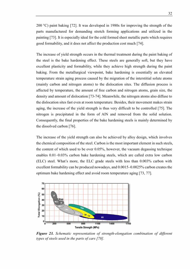
32
200 °C) paint baking [72]. It was developed in 1980s for improving the strength of the
parts manufactured for demanding stretch forming applications and utilized in the
painting [73]. It is especially ideal for the cold formed sheet metallic parts which requires
good formability, and it does not affect the production cost much [74].
The increase of yield strength occurs in the thermal treatment during the paint baking of
the steel is the bake hardening effect. These steels are generally soft, but they have
excellent plasticity and formability, while they achieve high strength during the paint
baking. From the metallurgical viewpoint, bake hardening is essentially an elevated
temperature strain aging process caused by the migration of the interstitial solute atoms
(mainly carbon and nitrogen atoms) to the dislocation sites. The diffusion process is
affected by temperature, the amount of free carbon and nitrogen atoms, grain size, the
density and amount of dislocation [73-74]. Meanwhile, the nitrogen atoms also diffuse to
the dislocation sites fast even at room temperature. Besides, their movement makes strain
aging, the increase of the yield strength is thus very difficult to be controlled [75]. The
nitrogen is precipitated in the form of AlN and removed from the solid solution.
Consequently, the final properties of the bake hardening steels is mainly determined by
the dissolved carbon [76].
The increase of the yield strength can also be achieved by alloy design, which involves
the chemical composition of the steel. Carbon is the most important element in such steels,
the content of which used to be over 0.05%, however, the vacuum degassing technique
enables 0.01–0.03% carbon bake hardening steels, which are called extra low carbon
(ELC) steel. What’s more, the ELC grade steels with less than 0.003% carbon with
excellent formability can be produced nowadays, and 0.0015–0.0025% carbon creates the
optimum bake hardening effect and avoid room temperature aging [73, 77].
Figure 23. Schematic representation of strength-elongation combination of different
types of steels used in the parts of cars [78].

33
The tensile properties of bake hardening steels are compared with other grades of steels
in Figure 23. The lower strength steels are in dark grey, and the high-strength steels (HSS)
are in light grey, the advanced high-strength steels (AHSS), which include Dual Phase
steel (DP steel), Complex Phase (CP) steel, Transformation Induced Plasticity (TRIP)
steel, Martensitic Steels (MS) are in colors. Bake hardening (BH) steels have low YS
value and good formability, which makes it ideal material for forming complex parts.
In the process of shape forming and paint baking, the occurrence of aging leads to
discontinuous yielding which increases yield strength. The yield strength increase of the
bake hardening steel is compared with the tensile behavior of mild interstitial free (IF)
steel and high strength rephosphorised steel in Figure 24. It shows that the bake hardening
steel can achieve both good shape and good dent resistance.
Figure 24. Schematic illustration of the behavior of bake hardening steel compared with
mild IF steel and rephosphorised steel [79].
Figure 25. Schematic representation of bake hardening response in tensile test [80].

34
Bake hardening steels exhibit an increase in yield strength after pre-straining. Figure 25
illustrates a typical bake hardening response of in the tension test after pre-straining. The
sharp yield strength, yield point elongation and modified work hardening behavior are
important features and properties [81]. The bake hardening behavior is measured in the
following process: the specimen is firstly pre-strained to 2% with tension at room
temperature, then be unloaded, aged at 170 °C for 20 min and then tensile tested again at
room temperature [82]. The bake hardening response is defined as the difference between
the lower yield stress after baking and the final flow stress after pre-straining, as shown
△σBH in Figure 25. De [83] found that the yield strength can be increased 30-40 MPa for
ultra-low carbon steels.
2.4.2 Mechanisms
The yield strength increase from the bake hardening is mainly attributed to the static strain
aging, which is essentially a diffusion process. The interstitial atoms (mainly carbon and
nitrogen atoms) migrate to the dislocation sites and lock the mobile dislocations, which
causes the increase of the yield strength via discontinuous yielding since the new mobile
dislocations are created to keep the plastic flow going on [84].
Conttrel and Bilby [64] firstly studied the theory and kinetics of dislocation pinning in
the strain aging, found that carbon atoms segregate to form the atmosphere around the
dislocations, which is called Conttrel atmosphere. Wilson and Russell [85-87] continued
the study on the strain aging, explored the theories and mechanisms of the strain aging,
and proposed the following stages of aging in the mild steels: (a) stress induced ordering
of interstitial atoms; (b) interstitial atoms segregation and dislocation locking by Cottrell
atmospheres; (c) formation and precipitation of solute cluster. The whole mechanism is
explained as below.
Snoek [88] studied the effect of small amount of carbon and nitrogen atoms on the iron’s
properties. He found that when the external force is applied on the material, the crystal
expands along the direction of the force, the interstitial atoms would migrate to occupy
the dislocation sites in the strain direction. While when the force is removed, the
interstitial atoms are distributed again randomly, which is the stress induced ordering, and
it’s also named “Snoek effect”. When the applied force exceeds the elastic limit of the
specimen, the new dislocations are produced. If such pre-strained material is then
thermally treated with aging at short time and higher temperature, the interstitial atoms
will migrate to these new dislocation sites and lock them by forming an atmosphere
around the dislocations, which is named Cottrell atmosphere [86-87].

35
With more and more solute atoms are attracted to the dislocation strain area, a solute
cluster can be formed, and in some extreme cases, when the solute cluster is strong enough,
it would make these interstitial atoms along the cores of dislocations [89]. Wilson and
Russell [87] also supported the above point. They found that the precipitates (carbide
particles for instance) would be coherent once they are formed. The process of bake
hardening is illustrated in Figure 26.
Figure 26. Schematic illustration of three stages in bake hardening [90].
Figure 27. Diagram of engineering stress-strain curve of low carbon steel demonstrating
the variation of dislocation and carbon atoms [91].
To gain a further understanding of how the bake hardening affects the properties of the
material, Kurosawa et al. [91] studied motion of solute carbon atoms and variation of
dislocations at different phases. It was found that, very few dislocations exist before the

36
external force is applied. With the increase of the force and pre-strain, more dislocations
are created, which produce work hardening effect. Afterwards, the bake-hardening heat
treatment enables more solute carbon atoms to move to the dislocation sites, while the
amount of dislocations is not significantly increased, the mobility of the dislocation is
reduced, which produce a bake hardening effect. These two hardening effects contributes
to the final yield strength increase of the material. Figure 27 illustrates the dislocation
situation of the specimen at different period of bake hardening treatment.
2.4.3 Kinetics of Bake Hardening
The bake hardening process, which consists of three stages of Snoek effect, Cottrell
atmosphere formation, and particle hardening (carbide precipitation), is essentially a
diffusion process. The carbide precipitation only occurs after the formation of Contrell
atmosphere, however, it is not accurate to simply understand the process by adding the
three periods, since the different influence of each stage on the bake hardening behavior
should be considered. Cottrell-effect is the most dominant stage among three stages,
which is restricted by the long time and high temperature, as shown in Figure 28.
Figure 28. Schematic presentation of the yield strength as a function of ageing time
during bake hardening process [80].
In theory, the increase of yield strength during bake hardening can be expressed as:
△σBH = △σSnoek + △σCottrell + △σPrecipitation (Eq 2)
Where △σSnoek, △σCottrell, and △σPrecipitation are the strength increments due to the Snoek
effect, Cottrell atmosphere, and carbides precipitation, respectively. However, Elsen and
Hougardy [74] considered that the final BH response is basically affected by two effects,
namely Cottrell atmosphere formation and the particle precipitation during bake
hardening. The curve above also shows that the Snoek effect has very slight effect on the

37
yield strength increment. Thus, the expression of the yield strength increment is:
△σBH =△σCottrell + △σPrecipitation (Eq 3)
However, this expression is just for a general understanding of the BH response, Elsen
and Hougardy did not consider the influence of solute atoms and other elements on the
yield strength increments. The influence of several factors on the bake hardening
responses are discussed in the next section.
2.4.4 Influence of Interstitial Atoms
As mentioned above, the bake hardening is essentially a diffusion process which relies on
the migration of the interstitial atoms. Thus, the content of the interstitial carbon and
nitrogen atoms has significant influence on the bake hardening. For BH steels, sufficient
“shelf life” is always necessary to ensure that the material would not undergo aging and
deteriorate in the transportation and storage before actual application. BH steels are
expected to have at least 3 months “shelf life”, and Bhagat’s study [92] about calculating
the “shelf life” of BH steel also exhibits a close relationship of the nitrogen and carbon
content with the “shelf life”. Nitrogen is especially deleterious since it diffuses rapidly
even at room temperature and makes aging and lead to the formation of Lüders bands
(stretcher strain), which should be avoided [75].
The BH response increases with the increase of solute carbon in the steel, since more
interstitial atoms are available and more solute can pin the dislocations, which forms
solute cluster more rapidly. Snick supported this [79], claiming that when the carbon
content increases from 0 to 40 ppm, the bake hardening responds a yield strength of 50-
80 MPa. However, it was noticed that the further increase of carbon content does not
increase the yield strength, and it would be stable at certain amount. Hainai et al. [93]
studied the effect of solid solution strengthening elements on the bake hardenability with
Al-killed steel which contained only 0.04% carbon content. They found that the increase
of yield strength reaches maximum when the sum of the content of carbon and nitrogen
is 20 ppm. However, that study did not reveal if the BH response can increase more when
the content of the solute atoms is over 20 ppm. Nevertheless, with the further increase of
carbon content, they would segregate and lock the dislocations even in the pre-straining
and reduce the BH response. This is demonstrated in Figure 29, in which ppm is short for
parts per million.

38
Figure 29. Yield strength increment as a function of free carbon content during bake
hardening response [79].
The effect of the increase of the carbon content on the room temperature aging and BH
response can also be understood by different levels of carbon content. Rubianes and
Zimmer [94] found that when the carbon content is no more than 3 ppm, steels are very
stable at room temperature and bake hardening is not shown, which is the regionⅠin the
Figure 30. When the carbon content is above 3 ppm while lower than 7 ppm, the steels
have good BH response from 20 to 60 MPa yield strength increase, and have resistance
to the room temperature aging. When the carbon content is over 7 ppm, the yield strength
increase is excellent, but it does not increase much with the further increase of carbon
content, whereas the room temperature aging is very likely to happen. Thus, BH grade
steels are supposed to be designed in region Ⅲ.
Figure 30. Yield strength increment as a function of carbon content in solution during
bake hardening response [94].
2.4.5 Influence of Pre-strain
Generally, many parts or components undergo small amount of straining during the
forming process or other processes before bake hardening. Thus, it is necessary to subject
the specimens to a small amount of pre-strain at room temperature, for the simulation of

39
the real situation. De et al. [95] studied the BH behavior of ultra-low carbon (ULC) steel,
they found that the maximum increase of yield strength at the end of Cottrell atmosphere
was the same for all the experimented pre-strain levels (1%, 2%, 5%, 10%), as shown in
Figure 31, the amount of pre-strain did not influence the Cottrell atmosphere formation.
The mechanism is the saturation of the dislocation sites, that the required Cottrell
atmosphere for saturation is the same for all dislocations and does not change with the
increase of dislocation density within strain range.
Elsen and Hougardy [80] studied the mechanism of bake hardening, and found the
increase of yield stress in the bake hardening contains two successive steps. The first step
is the Cottrell atmosphere formation, as discussed above. The second step is the carbides
precipitation. They also found the decrease of yield strength increment with the increase
of pre-strain level during the second step, which indicates that most carbon atoms
segregate to the dislocations at the first step.
Figure 31. Increase of yield strength of ultralow carbon steel with different pre-strains of
1%, 2%, 5%, and 10%, respectively [83].
De et al. [83] studied the dislocation density with ULC steel, and found the increase of

40
yield strength is mainly from the first step and not much from the precipitation step.
However, this is not applied to ELC steel, in which, the BH response is mainly from the
precipitation step. Tang et al. [96] studied the effect of pre-strain on the properties of TRIP
steel, finding that the yield strength increases markedly with the increase of pre-strain
within the range of 0 – 4%, while it increases slightly when the pre-strain ranges from 4%
to 16%. Kuang et al. [97] studied similarly with dual-phase steel, finding that the yield
strength increases obviously with increase of the pre-strain from 0% to 1%, while when
pre-strain ranges from 1% to 8%, the yield strength even decreases. Many similar studies
reveal that the effect of pre-strain level on the BH response is related to the material itself,
but a common result is that the BH response increases with the increase of pre-strain
within a very small range.
2.4.6 Influence of Baking Temperature and Time
Since the strain aging depends on the diffusion of interstitial atoms, temperature and time
are the dominant factors affecting the diffusion. Therefore, it is necessary to discuss the
effect of baking temperature and time on the strain aging.
De, et al. [83] studied the BH behavior of ULC steel with different aging time and
temperature, they found that the yield stress firstly increases with the baking time (or
aging time) until the yield strength increment reaches certain limit of 30-40 MPa, then
remains almost stable even the baking time continues increasing, the maximum increase
of yield stress is independent of aging temperature, which was shown in Figure 31.
Meanwhile, Figure 31 also illustrates that with the increase of baking temperature from
50 °C to 170 °C, the yield strength increases faster and reaches the stable yield strength
in shorter time, and this applies to different pre-strain levels.
Dehghani and Jonas [98] investigated dynamic-static bake hardening and dynamic bake
hardening, they found that both hardening achieve higher yield strength than the
conventional bake hardening. The scientists pre-strained the specimens at elevated
temperatures before bake hardening. Their results showed that the BH response is
remarkable when the baking temperature is higher than the pre-straining temperature,
while the BH response gets very slight when the baking temperature is lower than pre-
straining temperature. The mechanism for the latter case is that the relatively higher pre-
straining temperature causes massive interstitial atoms migration, Cottrell effect, and
carbide precipitation. However, the large amount of carbides limits the response in the
relatively low temperature bake hardening.

41
3 MATERIALS AND EXPERIMENTS
In this chapter, the experimental materials and procedures are introduced, the procedure
of micrographic observation is described and initial micrographs are presented. In
addition, the basis of tensile test data analysis is discussed and the principles for
determining bake hardening and aging indexes are presented.
3.1 Materials
The investigated materials consisted of three commercial steels: two low carbon steels
and a ferritic stainless steel (EN 1.4003). The samples of the carbon steels were provided
as tensile specimens by SSAB Europe Oy (Hämeenlinna). The samples of the EN 1.4003
ferritic stainless steels were provided by Outokumpu Oyj.
In this thesis, two low carbon steels are named steel A and steel B, EN 1.4003 ferritic
stainless steel is named steel C. The chemical analysis of the three experimental steels are
presented in Table 7. As indicated in the chemical composition, two low carbon steels
have quite similar chemical composition. The ferritic stainless steel (steel C) is
unstabilized, i.e., it is not alloyed with stabilizing elements Nb, Zr or Ti.
The steels A and B had been produced in the continuous production lines combining
continuous annealing and subsequent hot-dip galvanizing. Steel A had been annealed at
740 °C and steel B at 780 °C. The difference of the annealing temperature can cause the
difference of free carbon contents in the solution, which is vitally important to the bake
hardening behavior. The coiling temperature was the same, 720 °C, in both cases.
Table 7. Chemical compositions (% by weight) of three experimental materials.
Materials C Si Mn P S Al Cu Cr Ni N B
A 0.072 0.01 0.211 0.005 0.0092 0.024 0.021 0.249 0.035 0.0038 0.0016
B 0.073 0.015 0.223 0.009 0.01 0.036 0.017 0.301 0.041 0.0037 0.0021
C 0.013 0.34 1.36 - - - - 11.24 0.36 0.0057 -

42
3.2 Metallographic Observation
The initial microstructures of the test materials were investigated by using the optical
microscope. The cross-sectional samples of each material were prepared. The samples
were cut to both transverse and longitudinal directions with respect to the original rolling
direction. The metallographic observation of the specimens consists of two parts, namely
sample preparation and microstructure observation.
The sample preparation followed a standard procedure. The cross-sectional samples were
cut by using a cutting machine Struers Discotom-10. The sample pieces were then
mounted in epoxy in vacuum with machine Struers CitoVac. The samples were ground
with a number of grinding steps with sandpapers of different levels of smoothness (P320
– P600 – P800 – P1200 – P2000). In the operation, the sandpaper was fixed on the
spinning pan of the Buehler Phoenik 4000 sample preparation system, and the spinning
speed was set at 300 revolutions per minute (rpm) and force was set at 20 N, the specimens
were grinded with each sandpaper for 1 minute.
After grinding, polishing was performed with the same machine of grinding, the spinning
speed of the pan was 150 rpm, the force was 20 N, the polishing paper was changed every
30 seconds. The samples were polished with 3 µm and 1 µm diamond solutions, which
was applied every minute. The polishing was supposed to make the specimen surface
very smooth and bright.
Finally, for two low carbon steels, the specimen surface was etched with 4% nital for 6-
7 seconds; for ferritic stainless steel, the specimen surface was etched with etchant V2A
(100 ml water, 100 ml hydrochloric acid, 10 ml nitric acid), which was heated up to
around 80 °C. However, there were some problems when etching ferritic stainless steel.
Thus, only one image (transverse to the rolling direction) of the ferritic stainless steel is
presented in Figure 32. The etched sample surface was then examined with optical
microscope, and the microstructure pictures were taken.
Optical micrographs of the investigated steels in as-received condition are presented in
Figure 32. As can be seen, low carbon steels A and B consist primarily of ferrite and
randomly distributed cementite (the dark micro-constituent mostly at the grain boundaries
and intersection are of the grains in the pictures). Steel A and B also show very similar
microstructure. The grains of steel C are generally flatter and less evenly distributed than
the grains in steels A and B. In comparison, the microstructure of steel C shows smaller
amount of cementite due to lower carbon content.

43
Figure 32. Optical micrographs of the investigated steels: (a) A material of longitudinal
direction, (b) A material of transverse direction, (c) B material of longitudinal direction,
(d) B material of transverse direction, (e) C material (EN 1.4003 ferritic stainless steel)
of transverse direction.
The mean linear intercept method was used to measure the grain size of the initial
materials. Two optical images with 50× objective lens magnification of each material
were used, and eleven straight lines were made in each image, as shown in Figure 33. The
numbers of intercepts were counted, and the length of the lines were shown. Thus, an
average value of the grain size can be determined from each line. Therefore, there were
22 lines and 22 average values of grain size were available for each material. To eliminate
the error, the maximum and minimum values were deleted, and the remained 20 average

44
values were used to calculate the final average grain size (diameter) D by using the
following formula. The grain sizes of three as-received steels are presented in Table 8.
D = 1
20 * [
𝐿1
𝑛1 +
𝐿2
𝑛2 + … +
𝐿20
𝑛20] (Eq 1)
Figure 33. Illustration of the method of measuring grain sizes of initial materials.
Table 8. Grain diameters of as-received materials
Materials A B C
Grain Diameters (μm) 7.0 7.7 7.9
3.3 Bake Hardening Test
The as-received materials were subjected to bake hardening tests. The specimens were
first pre-strained to 0, 2, 6, or 10 %. After that, the pre-strained samples were subjected
to baking treatments of 170 °C/20 min and 230 °C/20 min. Finally, the mechanical
properties of the bake hardened specimens were determined with quasi-static tensile tests.
Each specimen was given a series number from 1 to 18, like A1 to A18, B1 to B18, and
C1 to C18. Then the specimens were classified according to the experimental plan, as
shown in Table 9. To eliminate the error from experiments and specimens, two specimens
were used for repeated experiments to determine the properties, the values of the
properties are the average values of the two results.

45
Table 9. Experimental plan for the bake hardening tests.
Steel A Steel B Steel C
No Bake Hardening A1, A2 B5, B6 C1, C2
170℃/20min A3, A4 B1, B2 C3, C4
230℃/20min A5, A6 B3, B4 C5, C6
2% pre-strain A7, A8, A9, A10 B7, B8, B9, B10 C7, C8, C9, C10
6% pre-strain A11, A12, A13, A14 B11, B12, B13, B14 C11, C12, C13, C14
10% pre-strain A15, A16, A17, A18 B15, B16, B17, B18 C15, C16, C17, C18
2% + 170℃/20min A7, A8 B7, B8 C7, C8
2% + 230℃/20min A9, A10 B9, B10 C9, C10
6% + 170℃/20min A11, A12 B11, B12 C11, C12
6% + 230℃/20min A13, A14 B13, B14 C13, C14
10% + 170℃/20min A15, A16 B15, B16 C15, C16
10% + 230℃/20min A17, A18 B17, B18 C17, C18
3.3.1 Tensile Testing
The tensile test specimens of the material A and B had been machined according to
international standard ISO 6892: 1998 (gauge width 20 mm). The testing direction was
perpendicular to the original rolling direction. The dimensions of the specimens are
described in Table 10. The dimensions of each individual tensile test specimen were
measured by a using a micrometer.
Table 10. Dimensions of the tensile specimens.
Carbon Steel Specimens Stainless Steel Specimens
Thickness t 0.55mm 1.97mm
Width of gage section W 1-6: 19.3mm
16mm Others: 16mm
Exceptions: B15-B18
Gage length G 120mm 120mm
Overall length L 25mm 23.5mm
Length of grip section B 30mm 30mm
Width of grip section c 50mm 43mm

46
However, after pre-straining and baking treatments the specimens were re-machined to
reduce the width of the gauge length to around 16mm, and the radius of the curvature was
reduced to 10mm. It was to avoid the localization of the necking occurring at the softer
area where the work hardening during pre-straining had not occurred. While there were
also exceptions like specimens B15 to B18, the machining was not successful with these
specimens in the first step. Thus, the gauge width was exceptionally small. The
dimensions before and after re-machining are presented in Appendix A.
Figure 34 shows an example of the tested specimen without re-machining. In this case,
the necking has localized to the softer non-pre-strained areas and resulted in the formation
of “banana-shaped” specimen, i.e., the necking has actually initiated on both sides of the
specimen. The observed phenomenon needs to the taken into account in the standard bake
hardening experiments.
Figure 34. Example specimen showing the necking at softer areas in pre-strained and
baked condition. The specimen was re-machined after pre-straining in order to avoid the
observed phenomenon.
Figure 35. Instron 8801 hydraulic testing machine [99].

47
Both pre-straining and final property testing were carried out with an Instron 8801 servo-
hydraulic testing machine, as illustrated in Figure 35. An extensometer (Instron 2630-100
Series) with a gauge length of 50 mm was used to measure elongation. The mechanical
properties in all conditions were determined using a quasi-static strain rate of 1 x 10⁻³ 1/s.
The same deformation rate was used in pre-straining. In all cases, two repetited tests were
carried out for reducing the influence of scatter and gaining more reliable results.
The extensometer was mounted on the surface of one side of the flat specimen, as
illustrated in Figure 36. The mechanical part transfers extension from the specimen to the
internal transducer via knife edges [100]. Since there is no relative movement between
the specimen and the extensometer when the extensometer is tightly fixed on the
specimen with the rubber band, the movement of the extensometer corresponds to the
movements of the specimen. To prevent the sharp edge cutting the rubber band, the edges
of hard and thick specimens are better to be wrapped with tape.
Figure 36. Schematic of strain measurement with clip-on extensometer [100].
The pre-straining and tensile testing were performed according to the specifications of
the EN-10002 tensile testing standard. During the pre-straining of the test pieces, the
testing rate was kept constant, and all tensile tests were performed by using the same
actual speed of the piston. In the case of carbon steels, the specimens were very thin by
thickness and were susceptible for small bending during closing the grips of the testing
machine. In the case of materials A and B, small tension was manually applied to avoid
bending of the specimens during closing the grips, which easily occurred for specimens
with a thickness of only 0.55 mm. After that, the testing was carried out in the same
manner as described above.

48
The data of piston position, load and strain were recorded during the tensile test. The
value of extensometer was balanced to zero before the test was started. However, the
extensometer was very sensitive with small external vibrations and thus, the value
differed slightly from zero. Consequently, the engineering strain was calculated as the
ratio of elongation to the original length, and it was given by:
ε = (εr – ε0) / (50 – ε0) (Eq 4)
Where εr is the recorded extensometer strain, ε0 is the initial strain of the extensometer
before testing, and 50mm is the gague length of the used extensometer.
The tensile stress is the ratio of normal stress to the cross section area. Thus, the
engineering stress can be calculated as follows:
σ = Fn / (t * w) (Eq 5)
Where Fn is the load (in N) at corresponding time, t is the thickness (in mm) of the cross
section, w is the width (in mm) of the cross section, thus, t*w gives the original cross
section size of the test piece. σ is the engineering stress in N/mm2, which corresponds to
MPa.
After that, the engineering stress-strain curves were calculated which allowed the
determination of mechanical properties. An example curve is shown in Figure 37. Tensile
strength is the highest point of engineering stress-strain curve. Uniform elongation is the
elongation corresponding to the ultimate tensile strength. The total elongation is the
elongation when the specimen is ruptured. The yield strength (YS), tensile strength (TS),
uniform elongation (UE), and total elongation A50 (the measuring gage length is 50 mm)
are the main properties of concern.
In some cases, a sharp yield point was appeared after bake hardening treatments. However,
in some cases, no sharp yield point was observed from stress-strain data. In such cases,
the 0.2% proof stress was used to determine the yield stress, i.e., 0.2% offset method was
applied, as illustrated in Figure 37. In these materials, the stress at which the material
switches from elastic deformation to plastic deformation is not easy to detect, thus, the
offset yield strength is determined. A straight line is constructed parallel to the initial
portion of the stress strain curve but offset by 0.2% from the origin point 0, as shown in
Figure 37. The 0.2% offset yield strength is the stress at the crossing point of the
constructed straight line and the actual stress-strain curve.
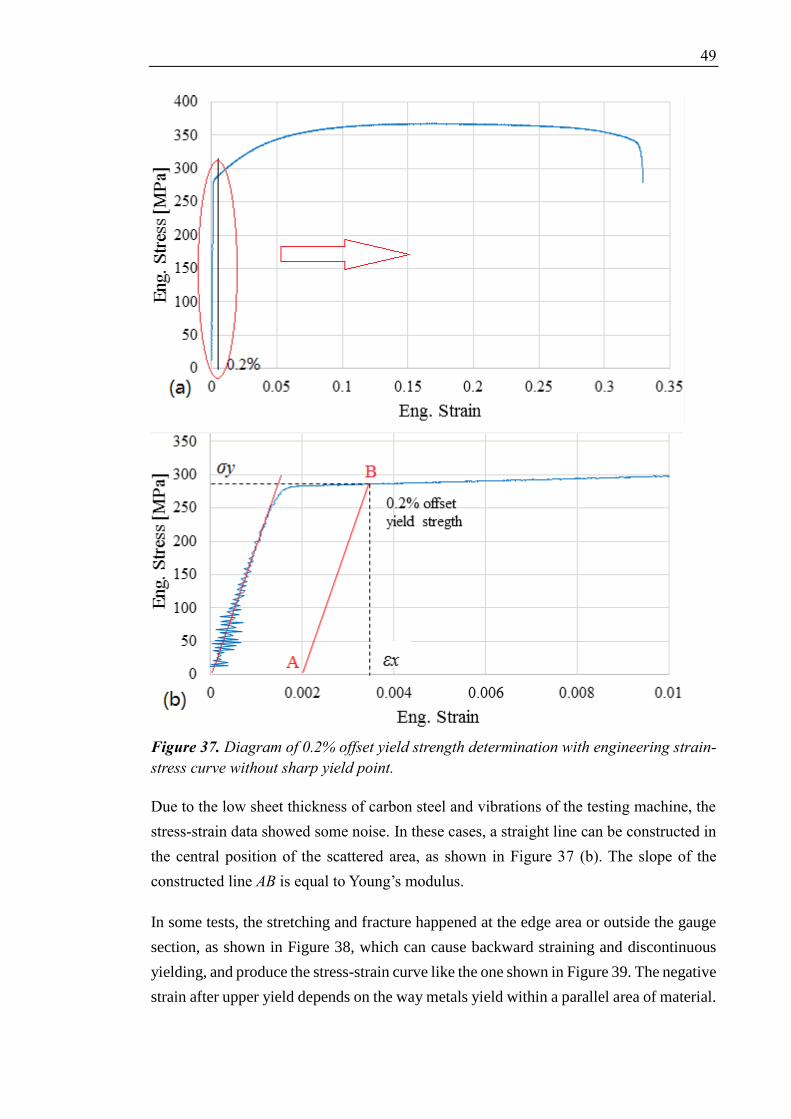
49
Figure 37. Diagram of 0.2% offset yield strength determination with engineering strain-
stress curve without sharp yield point.
Due to the low sheet thickness of carbon steel and vibrations of the testing machine, the
stress-strain data showed some noise. In these cases, a straight line can be constructed in
the central position of the scattered area, as shown in Figure 37 (b). The slope of the
constructed line AB is equal to Young’s modulus.
In some tests, the stretching and fracture happened at the edge area or outside the gauge
section, as shown in Figure 38, which can cause backward straining and discontinuous
yielding, and produce the stress-strain curve like the one shown in Figure 39. The negative
strain after upper yield depends on the way metals yield within a parallel area of material.

50
There is also stress concentration at the jaw faces in parallel specimens, and it would also
propagate through the steel in certain direction. The yielding takes place outside of gauge
section and lead to the stress drop, and makes tensile strength and corresponding uniform
elongation not available or not important any more.
Figure 38. Schematic diagram of tensile test piece in which the fractures are not in the
ideal gauge section.
Figure 39. Example of engineering stress-strain curve of the discontinuous yielding
specimens in the tests.
3.3.2 Bake Hardening Heat-treatments
The heat-treatment procedure of baking was carried out according to the standard EN
10325-2006 by using a fan-assisted furnace Thermo Scientific Heraeus. The specimen
temperature was measured with K-type thermocouples and a Fluke 52 thermometer, and
the thermocouple was attached to one reference specimen which was contacted with the
actual specimens. In the operation of heat treatment, the specimen was heated up to
170 °C or 230 °C in in the furnace. By the standard, the specimens are supposed to be
heated up to 168 °C (when aiming for 170 °C) within 5 min and heated up to 228 °C
(when aiming for 230 °C) within 7 min, respectively. All the specimens had been heated
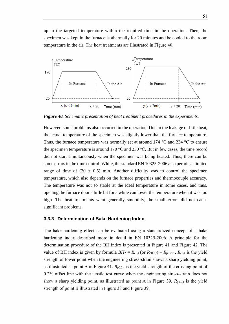
51
up to the targeted temperature within the required time in the operation. Then, the
specimen was kept in the furnace isothermally for 20 minutes and be cooled to the room
temperature in the air. The heat treatments are illustrated in Figure 40.
Figure 40. Schematic presentation of heat treatment procedures in the experiments.
However, some problems also occurred in the operation. Due to the leakage of little heat,
the actual temperature of the specimen was slightly lower than the furnace temperature.
Thus, the furnace temperature was normally set at around 174 °C and 234 °C to ensure
the specimen temperature is around 170 °C and 230 °C. But in few cases, the time record
did not start simultaneously when the specimen was being heated. Thus, there can be
some errors in the time control. While, the standard EN 10325-2006 also permits a limited
range of time of (20 ± 0.5) min. Another difficulty was to control the specimen
temperature, which also depends on the furnace properties and thermocouple accuracy.
The temperature was not so stable at the ideal temperature in some cases, and thus,
opening the furnace door a little bit for a while can lower the temperature when it was too
high. The heat treatments went generally smoothly, the small errors did not cause
significant problems.
3.3.3 Determination of Bake Hardening Index
The bake hardening effect can be evaluated using a standardized concept of a bake
hardening index described more in detail in EN 10325-2006. A principle for the
determination procedure of the BH index is presented in Figure 41 and Figure 42. The
value of BH index is given by formula BH2 = ReL,t (or Rp0.2,t) – Rp0.2,r . ReL,t is the yield
strength of lower point when the engineering stress-strain shows a sharp yielding point,
as illustrated as point A in Figure 41. Rp0.2,t is the yield strength of the crossing point of
0.2% offset line with the tensile test curve when the engineering stress-strain does not
show a sharp yielding point, as illustrated as point A in Figure 39. Rp0.2,r is the yield
strength of point B illustrated in Figure 38 and Figure 39.

52
Figure 41. Schematic illustration of bake-hardening index BH2 determination method
applied for low carbon steels.
Figure 42. Schematic illustration of bake-hardening index BH2 determination method
applied for ferritic stainless steels.
For the low carbon steel, a sharp yield point normally appeared after bake hardening in
the engineering stress-strain curve. Therefore, the BH index is determined with the yield
point and the stress when the pre-straining ends, as presented in Figure 41. For stainless
steel, there was no sharp yield point in the engineering stress-strain curve. Therefore, the
BH index was the determined by the difference of 0.2% offset yield strength after heat
treatment and 0.2% offset yield strength of the pre-strained material, which is the same
sample as tested after heat-treatment, as shown in Figure 42. The bake hardening index
is presented by plotting the engineering stress-strain curves with the data of the specimen
after heat treatment and the data of initial material.

53
3.4 Aging Index Test
In addition to bake hardening tests, an additional aging treatment was carried out in order
to evaluate the aging behavior during storage. In this procedure, two unstrained specimens
were hold in boiling water (100 °C) for 30 min and cooled in air to room temperature.
Quasistatic tensile tests were followed after the heat treatment. The aging indexes of this
type were determined by calculating the difference of the yield strength aroused by the
aging treatment. The treatment is illustrated in Figure 43. The aging indexes are
determined by calculating the difference of the yield strength aroused by the aging
treatment. The method of determining the index is the same as described in the Chapter
3.3.3.
Figure 43. Schematic diagram of aging treatment technology in the experiments.

54
4 RESULTS AND DISCUSSION
In this chapter, the initial properties of the three experimental materials are presented. In
addition, the results of the bake hardening tests and aging tests, which also include the
bake-hardening (BH) index determination result, are presented. In addition, the obtained
material behavior are discussed, and some findings are concluded.
4.1 Initial Properties
To study the initial mechanical properties of the experimental materials, two tensile tests
of each material were carried out. Engineering stress-strain curves were plotted and the
yield strength tensile strength, uniform elongation, and total elongation were determined.
Materials tested in as-received condition did not show sharp yield point, i.e., the point
where material behavior changes from elastic to plastic is relatively difficult to observe.
Thus, 0.2% offset method was used to describe yield strength of the materials in as-
received condition. TS is the ultimate tensile strength, uniform elongation is the
elongation corresponding to the ultimate tensile strength, and the total elongation is the
elongation when the specimen is ruptured. The initial properties of the experimental steels
are presented in Table 11.
Table 11. Initial mechanical properties of experimental materials.
YS 0.2%
(MPa)
(yield
strength)
UTS (MPa) Uniform
Elongation
Total
Elongation
Material A 285 370 17.5% 30.4%
Material B 277 367 18.6% 36.8%
Material C 409 519 15.6% 27.9%
As can be seen, the steel C (ferritic stainless steel) has higher initial strength than steel A
and B, while the initial yield strength and initial tensile strength of steels A and B are very
similar. However, the measures of elongation, especially the total elongation, of steel C
is slightly smaller than that of steels A and B. The mechanical properties are determined
by the combination of chemical composition and processing history of steels, both of
which has effect on the grain-size and phases present, for example. The stainless steel
contains higher carbon content, which enhances the hardness and strength of the material,

55
meanwhile, the high contents of chromium, nickel, silicon, and manganese also contribute
to the high strength. Das [73] reported that the higher annealing temperature improves the
bake-hardening response.
4.2 Bake Hardening Test Results
The experimental plan of each specimen was shown in the previous chapter in Table 9.
The principal idea followed in this thesis is to compare the tensile properties of as-
received condition with the ones after bake hardening treatments. Consequently, the
effect of pre-strain and baking temperature can be determined.
4.2.1 Effects of Bake Hardening
The effects of bake-hardening heat treatment without pre-straining can be determined by
comparing the mechanical properties of the initial status with those after the heat-
treatment. Appendix B presents the representative engineering stress-strain curves for
materials tested in initial condition and after bake hardening heat treatments without pre-
strain.
The effects of static strain aging, i.e., the bake hardening effect with pre-straining, can be
correspondingly determined by comparing the initial properties with the ones measured
after pre-straining and bake-hardening heat treatments. Appendix C presents the
representative engineering stress-strain curves showing the effect of bake hardening. In
this thesis, two different heat treatment procedures, namely 170 °C/20min and
230 °C/20min, and different pre-strain from 0% to 2%, to 6%, and to 10% were performed.
Two repeated tests were used to determine the values presented in Figures 45, 46, 48, and
49.
The YS values were determined in different methods depending on the characteristic of
the engineering stress-strain curve. When the yielding period was shown in the
engineering stress-strain curve, the YS value was determined based on the higher yield
point, as indicated with yield strength 1 in Figure 44(a). In case where sharp yield point
was not present, the 0.2% offset yield strength method was used to determine YS value,
as illustrated in Figure 44(b). There were also curves like Figure 44(c), in which the sharp
yield point was followed by a rapid reduction in strength and after that the strength level
was stabilized to a certain level. In such cases, the YS value was also determined with the
0.2% offset yield strength method, as indicated in Figure 44(c).

56
Figure 44. Illustration of yield strength value determination methods with different
engineering stress-strain curves.

57
Figure 45 presents the yield strength of the materials A and B at different status. The yield
strength values were determined by using higher yield point values, as indicated with
yield strength 1 in Figure 44(a).
Figure 45. Yield strength (determined with higher yield point) of steels A and B at initial
status and after different pre-straining and bake hardening treatments.
As can be seen in Figure 45(a), the 170 °C/20min heat treatment without pre-strain
resulted in an increase of 41 MPa in yield strength for both steels A and B. Figure 45(b)
indicates that 230 °C/20min heat treatment without pre-strain led to an increase of 135
and 130 MPa to steels A and B, respectively. At the meanwhile, with the 170 °C/20min
heat treatment, the increase of pre-strain level from 0% to 10% led to a △YS of 113 MPa
and 105 MPa to steels A and B, respectively. However, the △YS were 33 MPa and 28
MPa to steels A and B, respectively when baking temperature was 230 °C. Two low
carbon steels showed very similar yield strength with the increase of pre-strain under both
baking temperatures. The small difference of △YS at 230 °C is because the fact that
higher temperature without pre-strain is already enough to generate sharp yield point.

58
Figure 46 presents the lower yield strength values of the steels A and B, as indicated with
yield strength 2 in Figure 44(a).
Figure 46. Yield strength (determined with lower yield point) of steels A and B at initial
status and after different pre-straining and bake hardening treatments.
As indicated in Figures 45 and 46, the lower yield point values were increased similarly
with the increase of pre-strain. The values of yield strength determined with lower yield
point are generally lower than those determined with higher yield point, otherwise, no
significant difference in material behavior is shown between Figures 44 and 45.
The above-discussed results can be explained with the theories of SSA. According to
Pelleg [101], the interstitial atoms settle down under the dislocation line to form the
Cottrell atmosphere, and these atoms cause lattice distortion by forming a stress field
around themselves. However, the preferential location of the interstitial C and N atoms
below the dislocation is controlled by diffusion, which depends on the diffusion time and
temperature. When the atoms diffuse into the dislocation core, they stay there and pin the
dislocation, thus, a higher force is needed to tear such a dislocation away from its
atmosphere. This extra force corresponds to the upper yield point. After removing the
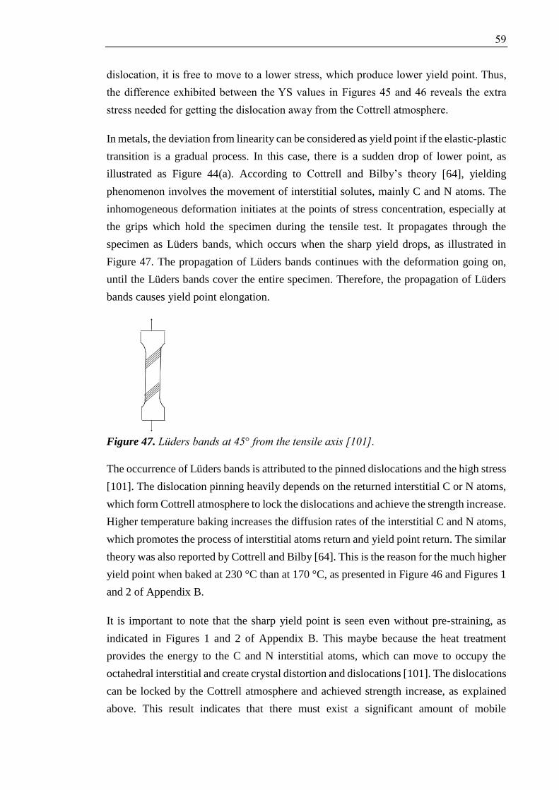
59
dislocation, it is free to move to a lower stress, which produce lower yield point. Thus,
the difference exhibited between the YS values in Figures 45 and 46 reveals the extra
stress needed for getting the dislocation away from the Cottrell atmosphere.
In metals, the deviation from linearity can be considered as yield point if the elastic-plastic
transition is a gradual process. In this case, there is a sudden drop of lower point, as
illustrated as Figure 44(a). According to Cottrell and Bilby’s theory [64], yielding
phenomenon involves the movement of interstitial solutes, mainly C and N atoms. The
inhomogeneous deformation initiates at the points of stress concentration, especially at
the grips which hold the specimen during the tensile test. It propagates through the
specimen as Lüders bands, which occurs when the sharp yield drops, as illustrated in
Figure 47. The propagation of Lüders bands continues with the deformation going on,
until the Lüders bands cover the entire specimen. Therefore, the propagation of Lüders
bands causes yield point elongation.
Figure 47. Lüders bands at 45° from the tensile axis [101].
The occurrence of Lüders bands is attributed to the pinned dislocations and the high stress
[101]. The dislocation pinning heavily depends on the returned interstitial C or N atoms,
which form Cottrell atmosphere to lock the dislocations and achieve the strength increase.
Higher temperature baking increases the diffusion rates of the interstitial C and N atoms,
which promotes the process of interstitial atoms return and yield point return. The similar
theory was also reported by Cottrell and Bilby [64]. This is the reason for the much higher
yield point when baked at 230 °C than at 170 °C, as presented in Figure 46 and Figures 1
and 2 of Appendix B.
It is important to note that the sharp yield point is seen even without pre-straining, as
indicated in Figures 1 and 2 of Appendix B. This maybe because the heat treatment
provides the energy to the C and N interstitial atoms, which can move to occupy the
octahedral interstitial and create crystal distortion and dislocations [101]. The dislocations
can be locked by the Cottrell atmosphere and achieved strength increase, as explained
above. This result indicates that there must exist a significant amount of mobile
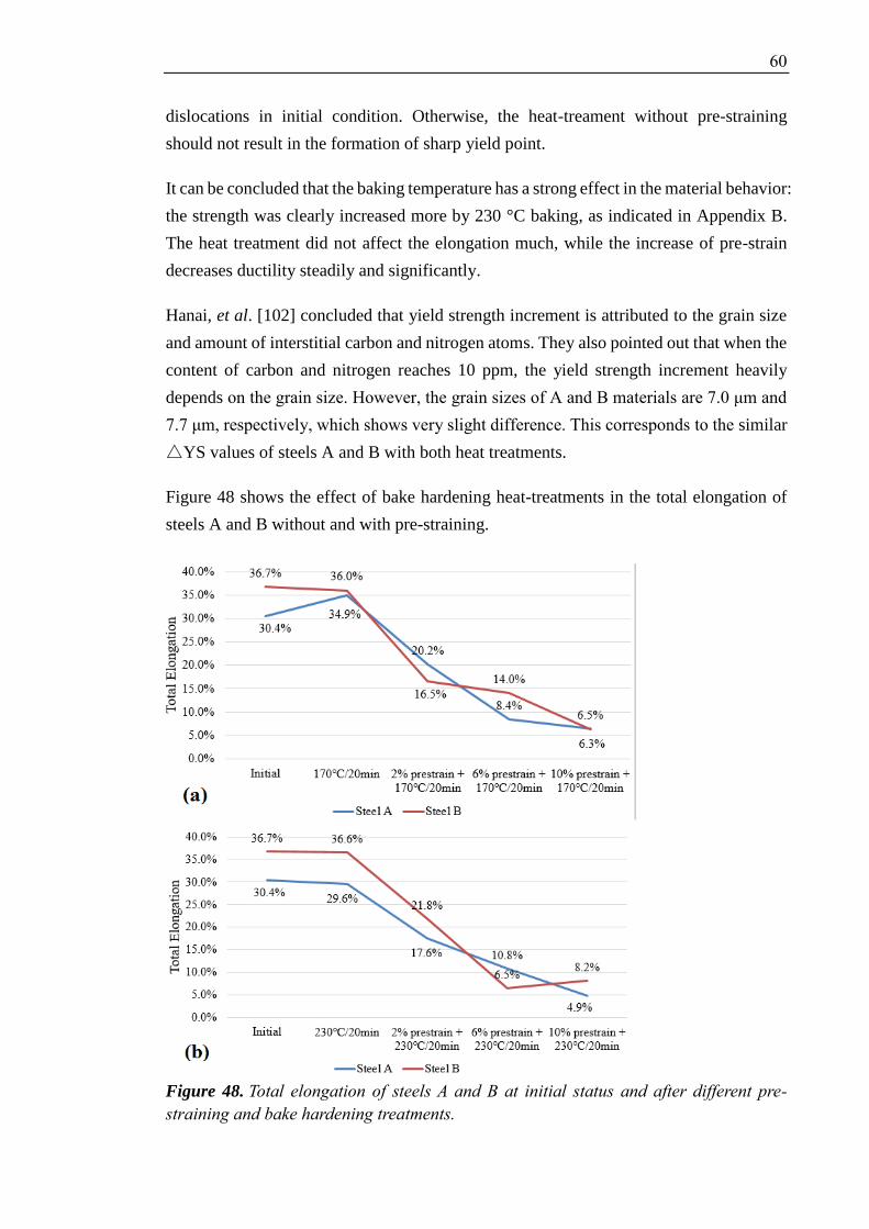
60
dislocations in initial condition. Otherwise, the heat-treament without pre-straining
should not result in the formation of sharp yield point.
It can be concluded that the baking temperature has a strong effect in the material behavior:
the strength was clearly increased more by 230 °C baking, as indicated in Appendix B.
The heat treatment did not affect the elongation much, while the increase of pre-strain
decreases ductility steadily and significantly.
Hanai, et al. [102] concluded that yield strength increment is attributed to the grain size
and amount of interstitial carbon and nitrogen atoms. They also pointed out that when the
content of carbon and nitrogen reaches 10 ppm, the yield strength increment heavily
depends on the grain size. However, the grain sizes of A and B materials are 7.0 μm and
7.7 μm, respectively, which shows very slight difference. This corresponds to the similar
△YS values of steels A and B with both heat treatments.
Figure 48 shows the effect of bake hardening heat-treatments in the total elongation of
steels A and B without and with pre-straining.
Figure 48. Total elongation of steels A and B at initial status and after different pre-
straining and bake hardening treatments.

61
Figures 47 and 48 indicate that the two steels exhibit very similar behavior when it comes
to the elongation behavior in general. The total elongation decreased steadily with the
increase of pre-strain as a result of both heat treatments, which indicates that the ductility
was decreased and strength was increased steadily with the increase of pre-strain.
However, the bake hardening treatment without pre-strain produced a small variation in
the total elongation of both steels A and B. Nevertheless, the variation was more
significant when the pre-strain was applied. This reveals that the pre-strain contributes
significantly to the work hardening phenomenon, which is related to the plastic
deformation, even work hardening also produces effect on the total elongation. In addition,
based on Figures 45, 46, and 48, it can be concluded that for the two low carbon steels,
the strength increased, the total elongation and ductility decreased with the increase of
pre-strain level. Seth had the similar finding with low carbon BH220 steel [74].
Figures 49 and 50 present the mechanical properties of steel C (EN 1.4003 ferritic
stainless steel) after different treatments. The YS values were determined with 0.2% proof
stress, since no sharp yield point was observed after bake hardening tests. This is the
reason why UTS and UE values were taken for steels C, but not for steels A and B.
Figure 49. Mechanical properties of steel C at initial status and after different pre-
straining and 170 °C/20min bake hardening treatment.

62
Figure 50. Mechanical properties of steel C at initial status and after different pre-
straining and 230 °C/20min bake hardening treatment.
Figure 49(a) indicates that in the case of steel C, 170 °C/20min heat treatment increased
a yield strength of 20 MPa and tensile strength 24 MPa of steel C. The impact of heat
treatments on the elongation of steel C is not as significant as that of steels A and B.
Besides, Figures 48 and 49(b) show that 170 °C/20min heat treatment without pre-strain
did not produce significant influence on the elongation of two low carbon steels, while it
produced a reduction effect on the uniform elongation and fracture elongation of steel C.
However, 230 °C/20min heat treatment had no significant influence on the elongation of
all three materials, as indicated in Figure Figures 48(b) and 50(b).
In comparison, Figure 50(a) shows that the △YS value of steel C is much smaller than
that of low carbon steels. Since the values for steel C are only 20 MPa and 3 MPa with
170 °C/20min and 230 °C/20min, respectively. The bake hardening effect is heavily
dependent on the diffusion of the interstitial atoms into the locations sites and Cottrell
atmosphere formation process [64]. However, the diffusion depends on the diffusion time
and temperature, which is essentially related to the energy provided [101]. In addition,
the amount of mobile dislocations in initial condition can have an effect. The small

63
increase in the yield strength of steel C reveals that the diffusion of interstitial atoms in
the stainless steel requires higher energy than the two low carbon steels. Similar result
was also reported by Palosaari, et al [103], who found that activation energies for EN
1.4509 and EN 1.4521 ferritic stainless steels are 150.7 KJ/mol and 146.3 KJ/mol,
respectively, which are greater than that of ultra-low carbon bake hardenable steels, 80
KJ/mol.
To study the effect of different level of pre-straining, pre-strains of 2 %, 6% and 10 %
were applied and followed with the baking at 170 °C and 230 °C for 20 min. The
engineering stress-strain curves for the specimens with different pre-strain and same bake
hardening are presented in Appendix C. Figures 49 and 50 suggest that for EN 1.4003
ferritic stainless steel, with the same bake-hardening treatment, the tensile strength
increased, while the elongation and ductility decreased with the increase of the level of
pre-strain. This result is also applied to the two low carbon steels.
Figure 45, 46, 49, and 50 show that for the three experimental materials, the △YS values
were reduced when the pre-strain increased from 6% to 10%, in comparison with the
increase between 2% and 6%. Lower level of pre-strain naturally leads to the smaller
amount of mobile dislocations. However, the amount of free C and N is always limited.
It is possible that with higher pre-strain values, there was not sufficient free interstitial
atoms to lock dislocations. Besides, the increased work hardening response in greater
when the pre-strain increased from 2% to 6%, in comparison with the response between
6% to 10% pre-strain, as illustrated in Figure 51. Work hardening also contributes to the
△YS value. However, with higher level of pre-strain, higher dislocation density makes
the solute atoms insufficient to provide pinning for all dislocations [104].
Figure 51. Illustration of the bake-hardening indexes determination. Tensile test
specimens: B9 (2% pre-strain and 230 °C/20min), B13 (6% pre-strain and 230 °C/20min),
B17 (10% pre-strain and 230 °C/20min).
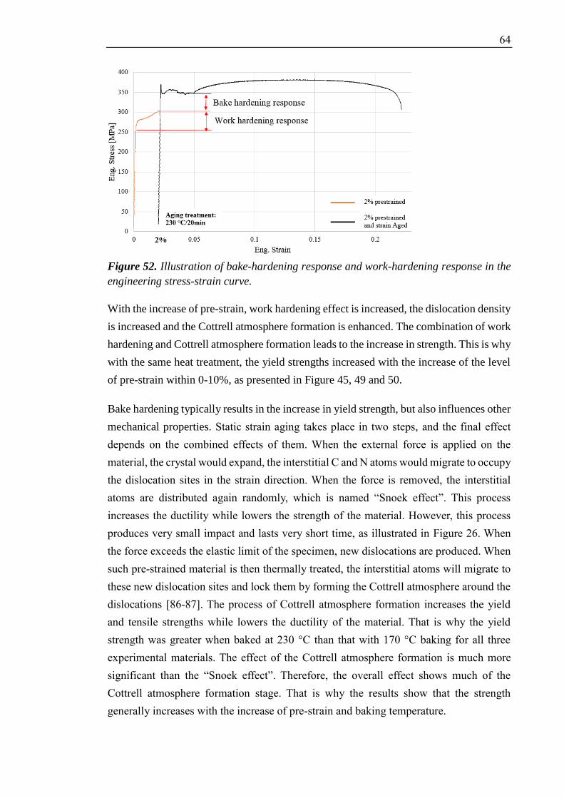
64
Figure 52. Illustration of bake-hardening response and work-hardening response in the
engineering stress-strain curve.
With the increase of pre-strain, work hardening effect is increased, the dislocation density
is increased and the Cottrell atmosphere formation is enhanced. The combination of work
hardening and Cottrell atmosphere formation leads to the increase in strength. This is why
with the same heat treatment, the yield strengths increased with the increase of the level
of pre-strain within 0-10%, as presented in Figure 45, 49 and 50.
Bake hardening typically results in the increase in yield strength, but also influences other
mechanical properties. Static strain aging takes place in two steps, and the final effect
depends on the combined effects of them. When the external force is applied on the
material, the crystal would expand, the interstitial C and N atoms would migrate to occupy
the dislocation sites in the strain direction. When the force is removed, the interstitial
atoms are distributed again randomly, which is named “Snoek effect”. This process
increases the ductility while lowers the strength of the material. However, this process
produces very small impact and lasts very short time, as illustrated in Figure 26. When
the force exceeds the elastic limit of the specimen, new dislocations are produced. When
such pre-strained material is then thermally treated, the interstitial atoms will migrate to
these new dislocation sites and lock them by forming the Cottrell atmosphere around the
dislocations [86-87]. The process of Cottrell atmosphere formation increases the yield
and tensile strengths while lowers the ductility of the material. That is why the yield
strength was greater when baked at 230 °C than that with 170 °C baking for all three
experimental materials. The effect of the Cottrell atmosphere formation is much more
significant than the “Snoek effect”. Therefore, the overall effect shows much of the
Cottrell atmosphere formation stage. That is why the results show that the strength
generally increases with the increase of pre-strain and baking temperature.

65
When more and more interstitial atoms are attracted to the dislocation strain area, a solute
cluster can be formed, and in some extreme cases, when the solute cluster is strong enough,
these interstitial atoms would be along the cores of dislocations [89]. As indicated in
Figure 26, no particle hardening phase is present during the Cottrell atmosphere formation
period. However, the particle hardening effect is increased rapidly when the aging
continues after Cottrell atmosphere formation. Nevertheless, this particle hardening effect
would reach a saturation point, after which further aging would reduce the particle
hardening phases.
4.2.2 Bake-Hardening Index Determination
The method for determining BH index was introduced in Chapter 3.3.3. As discussed
earlier, several kinds of yielding behavior and engineering stress-strain curves appeared
during tensile tests. In the case of low carbon steels (steels A and B), the bake hardening
treatments resulted in the formation of sharp yield point, whereas the stress-strain curves
measured for ferritic stainless steel (steel C) did not show this phenomenon. For these
two categories, the BH indexes were determined by the illustrated methods, which is also
approved by the standard EN 10325: 2006. In some cases, the stretching and fracture
happened at the edge area or outside the gauge section, and caused backward straining
and discontinuous yielding, their stress-strain curves are like the one shown in Figure 39.
For these curves, the 0.2% offset yield strength method was applied to determine the yield
strength.
The BH indexes of ferritic carbon steels (steel A and B) are presented in Figure 53 and
54. Appendix D presents the detailed data of BH indexes of three materials. The
determined BH indexes of two ferritic carbon steels are quite similar. With the
170 °C/20min heat treatment, the BH indexes of two low carbon steels increased from
around 19 MPa to around 54 MPa steadily with the increase of pre-strain from 0% to 10%.
However, with the 230 °C/20min heat treatment, the BH indexes of two low carbon steels
decreased from around 70 MPa to around 58 MPa steadily along with the increase of pre-
strain from 0% to 10%. The two low carbon steels exhibited very similar behavior in
terms of BH indexes.
Figures 53 and 54 also reveal that the values of BH index are greater with higher baking
temperature, especially when the pre-strain level is low. It is because the higher baking
temperature provided greater thermal energy, which increased the diffusion rate of the
carbon atoms in the material. As a result, the interaction of dislocations and interstitial
carbon atoms was increased and greater yield strength increment was achieved.

66
Figure 53. Bake-hardening indexes for steel A with two bake-hardening heat treatments.
Figure 54. Bake-hardening indexes for steel B with two bake-hardening heat treatments.
Figures 53 and 54 illustrate that when baking temperature was 230 °C, BH indexes follow
a general decreasing trend with the increase of pre-strain. This is because the high
temperature provided sufficient thermal energy, which increased the diffusion rate of
interstitial C atoms into the dislocation cores. However, with the increase of pre-strain,
larger amount of dislocations were produced, but the work hardening effect is less
increased with the further increase of pre-strain, as indicated in Figure 51. Thus, there
was not very significant increase of the amount and density of dislocations even the pres-
train was increased further to 10%. The maximum point of the Cottrell atmosphere
formation had been reached or was very close, the further increase of pre-strain led to
lower ΔYS value.
However, when baking temperature was 170 °C, BH indexes followed the trend of BH2
< BH6 < BH10, which is opposite to the case when baking temperature was 230 °C. Since
at lower temperature of 170 °C, the interstitial atoms diffused slowly due to the lack of
thermal energy. The dislocation density with the same level of pre-strain are supposed to
be the same. However, the Cottrell atmosphere formation saturation point had not been

67
reached when baked at 170 °C due to the low diffusion process. Thus, when the pre-strain
was increased, larger amount of dislocations were available for the mobile C atoms to
diffuse into. Thus, higher ΔYS value was achieved.
Das, et al. [105] reported the same phenomenon that the ΔYS decreases with the increase
of pre-strain level. This is because the aging condition did not give sufficient time to
ensure the dislocation pinning to be completed. This is consistent with the earlier findings
of Cottrell and Bilby [64]. De, et al. [83] found that maximum increase in yield strength
corresponding to the completion of Cottrell atmosphere formation on the dislocations
depends on the level of pre-strain, while increasing baking temperature can only improve
the maximum ΔYS value slightly. Therefore, there is certain “saturation” point when the
Cottrell atmosphere has been at or around the dislocations and the further increase of pre-
strain level can hardly produce strength increase effect. The phenomenon of BH2 > BH6 >
BH10 when baking temperature was 230 °C is attributed to this.
The BH indexes for EN 1.4003 ferritic stainless steel (steel C) are presented in Figure 55.
With 170 °C/20min heat treatment, ΔYS was decreased when pre-strain increased from
0% to 2%, which is probably due to the specimen scattering. The BH index was increased
very slowly along with the increase of pre-strain from 2% to 6%, while it increased
remarkably when the pre-strain was increased up to 10%. In comparison, the BH index
increased more significantly, from 8 MPa to 32 MPa, with the increase of pre-strain from
0% to 10% when baked with 230 °C. Palosaari, et al. [3] also found that the BH indexes
of three ferritic stainless steels increased with the increase in aging temperature between
150 °C and 250 °C. This is attributed to its high activation energy, higher temperature
provides greater thermal energy, which promote the diffusion of solute atoms more and
achieve more significant strain aging. However, low temperature could hardly provide
sufficient energy for the diffusion of interstitial atoms and Cottrell atmosphere formation.
Figure 55. Bake-hardening indexes for steel C with two bake-hardening heat treatments.

68
The comparison between Figures 53-54 and Figure 54 reveals that, the values of BH index
of low carbon steels are significantly greater than that of ferritic stainless steel. This
indicates that the heat treatment and pre-strain generally produce greater effect on the
ΔYS of low carbon steels than ferritic stainless steel. Besides, the index BH0 of low
carbon steels are distinctly greater than that of ferritic stainless steel, the BH0 values of
low carbon steel with two heat treatments are around 72 MPa, while the BH0 values of
EN 1.4003 ferritic stainless steel are 26 MPa with 170 °C/20min heat treatment and 8
MPa with 230 °C/20min heat treatment, respectively. BH index reveals the susceptibility
to static strain aging during paint-baking of the material. Thus, it can be revealed that the
low carbon steels exhibit stronger bake hardening effect than the stainless steel, at least
within 170 °C.
However, it is also noticeable that for the two low carbon steels, with the increase of pre-
strain from 0% to 2%, BH index was increased rapidly with both baking temperatures.
However, also with the both baking temperatures, the BH index was increased at slower
rate along with the further increase of pre-strain. It is possible to predict that if greater
level of pre-strain, like 12% and 14%, a very small or almost no increase of BH index
would be seen [96-97].
Kuang, et al. [97] reported similar result when experimented with dual-phase steel, they
pointed out that, the effect of pre-strain on the bake-hardening index contains two stages,
when the pre-strain increases within very small range, △σBH increases rapidly, whereas
when pre-strain exceeds certain range and continues increasing, the △σBH value is
decreased. The same behavior was also found by Tang et al, [96] the bake hardening
behavior of the Si-Al-Mn TRIP steel showed that, the △σBH value increases with the
increasing pre-strain within 0-4%, but the △σBH value decreases when the pre-strain
increases over 4%.
The increase of pre-strain increases the amount of mobile dislocations in the matrix. In
this case, the high density of dislocations makes atoms migration easier by eliminating
the diffusion distance between carbon atoms and free dislocation sites. Therefore, the
increase in dislocation density increases the amount of dislocation pinning effect, which
leads to the significant increase of BH index.
There is a maximum △σBH value with certain pre-strain, which is attributed to the
maximum value of the degree of Cottrell atmosphere formation, above which the further
increase of pre-strain does not lead to significant increase of Cottrell atmosphere
formation [106]. When the mobile dislocations are saturated or the process is limited due

69
to the lack of sufficient interstitial C atoms. This is the reason for the decrease of △σBH
value with high degree of pre-strain. Ferritic stainless steel exhibited differently that the
△σBH value continues increasing with the increasing pre-strain, since the mobile
dislocations had not been saturated. A critical degree of Cottrell atmosphere formation
had not been reached even with 10% pre-strain. It can be predicted that with greater pre-
strain, it will probably show similar decreasing trend as well.
Higher temperature accelerates the diffusion kinetics, which promotes the migration and
diffusion of C and N atoms, thus, increasing the Cottrell atmosphere formation, and
strengthening effect. That is why the △σBH values were greater when baked at 230 °C
than those when baked at 170 °C. The same result and behavior were also found by Kuang,
et al [97].
4.3 Aging Test Results
Representative stress-strain curves used in aging index determination are presented in
Appendix E. In Figure 1 of Appendix E, the engineering stress-strain curve of initial steel
A shows around shape, whereas the curve is slightly different after strain aging treatment.
However, in Figure 2 of Appendix E, the engineering stress-strain curve of initial steel B
shows the same shape as the curve of aged steel A (curve AI-A2), and the aged steel B
(curve AI-B1) shows no difference from the curve of initial steel B. This suggest that the
steel B had already aged a little bit at room temperature before 100 ˚C/30 min treatment,
however, that temperature was not enough to produce more aging effects.
The results of the aging index determination of two low carbon steels are shown in Figure
56 and 57. It can be seen that the aging treatment led to a very slight decrease in strength
and increase in elongation of two low carbon steels, but it practically produced no
significant influence on the properties.

70
Figure 56. Mechanical properties of steel A before and after 100 °C/30 min aging
treatment.
Figure 57. Mechanical properties of steel B before and after 100 °C/30 min aging
treatment.
The results of the aging index determination of EN 1.4003 ferritic stainless steel are
shown in Figure 58. The result is very similar to that of low carbon steels that the
100 °C/30 min aging treatment produced no significant influence on the properties.

71
Figure 58. Mechanical properties of steel C (1.4003 ferritic stainless steel) before and
after 100 °C/30 min aging treatment.
During the heat treatment of 100 °C/30min, the dislocations are recovered to some extent,
which in a general level reduces strengths and improves ductility. On the other hand, the
dislocations on the grain boundaries are pinned when the carbon migrates towards
dislocations, which strengthens the material and decreases the ductility. These processes
compete, and the result determines the final effect of aging treatment on the properties. It
is most probably that in the ferritic stainless steel, higher temperature and higher
activation energy are needed to activate carbon, the 100℃ heat treatment is not sufficient
to migrate lots of carbon towards dislocation, M. Palosaari et al. [3] also found that
activation energies for similar ferritic stainless steels are higher than that for ultra-low
carbon bake hardenable steels.
In can be concluded that the aging temperature 100 °C was too low to cause significant
aging. The slight increase of the total elongation is most probably aroused by natural
scatter in material properties and tensile testing. 100 °C heat treatment is probably not
sufficient to provide sufficient energy to activate the free carbon and nitrogen atoms to
move. Thus, it suggests that the investigated low carbon steels and ferritic stainless steel
are not susceptible to room temperature during storage.
72
4.4 Discussion of Errors and Future Work
4.4.1 Possible Sources of Errors
First of all, the small differences in the dimensions, compositions, mechanical properties
exist among the specimens of the same material. However, the effects on the mechanical
properties of the heat treatment and aging treatment are based on different specimens. For
example, in Figure 55, the initial properties of C material were determined from two
specimens of C material, whereas the properties after aging treatment are from another
two C specimens. There can be small difference between these specimens. This error
source has also been reported by Gabauer [107], who suggested that the shape and size
of specimen and dimensional compliance all produce error in the tensile testing. But in
this case, it is not practical to use the same specimen for both experiments. Thus, taking
the average value of the results of two specimens has decreased the influence due to
scattering.
Secondly, the influence on the data accuracy can also be from the testing data, which can
be caused by the extensometer measurement. For example, the vibration of tensile testing
machine generated noise to the measured data, which produces scattering curve and
reduces the accuracy of the yield strength determination. In addition, the rubber band was
used for fixing the extensometer on the specimen surface. However, the stainless steel
specimens had very smooth surface and sharp edges. Therefore, to prevent the
extensometer slipping in the testing and to prevent the rubber band being broken by the
sharp edge, the tape was used between the extensometer and specimen surface. However,
this can also reduce the accuracy of the result, especially when the rupture happens to or
near the tape.
Some specimens did not exhibit ideal behavior during the tensile tests, as indicated in
Figure 36. The backward straining and discontinuous yielding occurred in some tensile
tests, which make it difficult to determine the properties. Scattering also happened when
some test pieces were subjected to the tensile tests, which influences the accuracy of the
data. Some errors also occur in the operation. For example, the sample cutting and
grinding can cause stretches on the specimen surface, etching can all influence the surface
condition, which consequently influence the microstructure. Errors can also come from
the operation of heat treatment and tensile tests, which all influence the material behavior
and properties. The errors can be reduced by using repeated experiments, while they
cannot be avoided completely.

73
4.4.2 Further Work
In this study, the static strain aging behavior of selected ferritic steels was investigated by
as a function of aging temperature and the amount of pre-strain. Further studies could
address, for example, investigating the influence of aging time on the strain aging
behavior and properties of the material, Palosaari, et al. [3], De, et al. [104], Vasilyev, et
al. [108] have done the research in this field. They found that the strength increases with
the increase of aging time within certain limit, while the further increase of aging time
does not increase the strength more, or even leads to a decrease of strength. In order to
understand the SSA phenomena in general, the influence of aging time on the material
behavior can be investigated.
In addition, the effect of individual alloying elements on the bake hardening behavior
could be investigated. Pereloma, et al [109] reported that the addition of chromium
produced significant influence on the aging process. Similar research can be done to gain
further understanding on how some specific elements affect the aging process and
properties of the materials, and it would also give suggestion on the control of strain aging
process.

74
5 CONCLUSIONS
Bake hardening behavior of two low carbon steels and a ferritic stainless steel (EN 1.4003)
were investigated. The most important findings are summarized as below.
(1) It is necessary to reduce the width of the specimens after pre-straining and baking,
before final tensile tests, in order to avoid the localization of the necking occurring
at the softer areas outside the gauge section, i.e. areas between the grip sections
and gauge section of the specimen.
(2) For the two low carbon steels, the strength was increased significantly with the
increase of and baking temperature from 170 °C to 230 °C. However, the increase
of pre-strain level from 0% to 10% also led to smaller strength increment.
(3) For EN 1.4003 ferritic stainless steel, 170 °C/20min and 230 °C/20min heat
treatments led to slight strength increase. However, the increase of pre-strain level
from 0% to 10% led to significant strength increase.
(4) Two low carbon steels exhibited very similar BH indexes in all cases. With the
increase of pre-strain level from 0% to 10%, the BH indexes of two low carbon
steels increased steadily and significantly from around 19 MPa to 54 MPa when
baked at 170 °C, while they decreased steadily from around 70 MPa to 58 MPa
when baked at 230 °C.
(5) With the increase of pre-strain level from 0% to 10%, the BH index of EN 1.4003
ferritic stainless steel increased not significantly when baked at 170 °C, but it
increased steadily from 8 MPa to 32 MPa when baked at 230 °C. The BH index
of two low carbon steels were significantly greater than that of EN 1.4003
stainless steel, which is due to the higher activation energy of EN 1.4003 ferritic
stainless steel than the low carbon steels.
(6) 100 °C/30min aging treatment did not produce significant influence on the
properties of three investigated ferritic steels.

75
REFERENCES
[1] Y. Y. Yan, F. L. Lian, G. F. Liang, et al., “An Overview of Strain in Low Carbon
Steels,” Baosteel Technical Research, Vol.8, No.2, pp.58-64, June 2014.
[2] A. Banerjee and S. K. Dhal, “Effect of Strain Ageing in Welded and Non-welded
Low Carbon Steel,” Bachelor’s thesis, Dept. Metall. & Mater. Eng., Nat. Inst. of
Tech., Rourkela, India, 2010.
[3] M. Palosaari, T. Manninen, R. Toppila, et al., “Static Strain Aging of Stabilized
Ferritic Stainless Steels,” in Proc. 7th European Stainless Steel Conference, Como,
Italy, September 21-23, 2011, W. Nicodemi, J. O. Nilsoon, A. Tiziani, Eds.
Milano, Italy: La Metallurgia Italiana, Vol.104, No.9, 2012. pp. 25-28.
[4] V. T. L. Buono, B. M. Gonzalez, and M.S. Andrade, “Strain Aging of AISI 430
Ferritic Stainless Steel,” Scrip Materialia, Vol.38, No.2, pp. 185-190, Dec. 1997.
[5] B. L. Bramfitt, A. O. Benscoter. “Introduction to Steels and Cast Irons,” in
Metallographer’s Guide: Practices and Procedures for Irons and Steels, Materials
Park, Ohio: ASM International, 2002, pp. 1-21.
[6] R. Singh, Applied Welding Engineering (Second Edition): Process, Codes, and
Standards. Oxford: Butterworth-Heinemann, 2016, p.33,
[7] D. T. Liewellyn and R. C. Hudd, “Low Carbon Strip Steels” in Steels (Third
Edition): Metallurgy and Applications, Oxford: Butterworth-Heinemann, 1998,
pp. 1-136.
[8] H. M. Cobb (Ed.), Appendix I: Metals History Timeline, in Dictionary of Metals,
Materials Park, Ohio: ASM International, 2012, p.304.
[9] B. Boulet, G. Lalli, and M. Ajersch, “Modeling and Control of an Electric Arc
Furnace,” in Proceedings of the 2003 American Control Conference, Denver,
Colorado, USA, June 4-6, 2003. Vol.4, July 2003, pp. 3060-3064.
[10] “Understanding the Benefits of Electric Arc Furnace Technology for Ceramics,
Refractories, and Other Industries,” Ceramic Industry Magazine, April 2015, pp.
33-34.

76
[11] J. Madias, “Electric Furnace Steelmaking,” in Treatise on Process Metallurgy,
Volume 3: Industrial Process, S. Seetharaman, A. McLean, R. Guthrie, et al., Ed.
Oxford: Elsevier, 2014, pp. 271-300.
[12] Y. X. Yang, K. Raipala, and L. Holappa, “Ironmaking,” in Treatise on Process
Metallurgy, Volume 3: Industrial Process, S. Seetharaman, A. McLean, R.
Guthrie, et al., Ed. Oxford: Elsevier, 2014, pp. 1-89.
[13] K. I. Satyendra, “Importance of Hearth, Deadman and Tapping in Blast Furnace
Operation,” Ispat GURU, April 13, 2016. [Online]. Available: http://ispatguru.
com/importance-of-hearth-dead-man-and-tapping-in-blast-furnace-operation/.
[Accessed April 19, 2017].
[14] Stahl-Zentrum, “Hot Metal and Crude Steel Production,” Steel Institute VDEh,
German Steel Federation, [Online], Available: http://en.stahl-online.de/index.
php/topics/technology/steelmaking/. [Accessed April 19, 2017]
[15] M. M. Wolf, “History of Continuous Casting,” in 75th Steelmaking Conference
Proceedings, Toronto, Canada, April 5-8, 1992, Warrendale, PA: Iron & Steel
Society, 1992, pp. 83-137.
[16] B. G. Thomas, “Continuous Casting,” in Moelding for Casting and Solidification
Processing, New York: Marcel Dekker Inc, 2002, pp. 499-540.
[17] R. Singh, “Classification of Steels,” in Applied Welding Engineering (2nd Edition):
Process, Codes, and Standards, Amsterdam: Elsevier Inc, 2016, pp. 57-64.
[18] B. J. Hewitt, “High Convention Hydrogen Batch Annealing in British Steel,” in
Review of Annealing Technology, Technical Exchange Session, Brussel, Belgium,
May 3-4, 1995, Brussel, Belgium: Int. Iron and Steel Inst., 1995. p. 51.
[19] M. Imose, Heating and Cooling Technology in the Continuous Cooling. Trans.
ISIJ, Vol.25, pp. 911-932, 1985.
[20] D. Gandy, Carbon Steel Handbook (1014670). Palo Alto, CA: Electric Power
Research Institute, Inc, 2007.
[21] C. C. Anya and T. N. Baker, “The Effect of Silicon on the Grain Size and the
Tensile Properties of Low Carbon Steels,” Mater. Sci. Eng. Sec. A, Vol.118, pp.
197-206, Oct. 1989.

77
[22] A. C. Reardon, “Steel Product and Properties,” in Metallurgy for the Non-
Metallurgist, 2nd Edition, Materials Park, Ohio: ASM International, 2011, pp. 175-
196.
[23] G. Krauss, “High-Carbon Steels: Fully Pearlitic Microstructures and
Applications,” in Steel: Processing, Structure, and Performance. Materials Park,
Ohio: ASM International, 2005, pp. 281-295.
[24] High Carbon Steels, Total Materia. Updated: April 2012. [Online] Available:
http://www.totalmateria.com/page.aspx?ID=CheckArticle&site=kts &NM=368.
[Accessed: June 13, 2016].
[25] B. Capudean, “Metallurgy Matters: Carbon Content, Steel Classifications, and
Alloy Steels,” Practical Welding Today, August 2003. [Online]. Available: http://
www.thefabricator.com/article/metalsmaterials/carbon-content-steel-
classifications-and-alloy-steels. [Accessed June 14, 2016].
[26] E. Lugscheider, “Constitution and properties of steels,” Edited by F. B. Pickering,
in Vol.7 of Materials Science and Technology—A Comprehensive Treatment. R.
W. Cahn, P. Haasen, E. J. Kramer, Eds. Weinheim: Wiley-VCH, 1991, p.7, 41.
[27] C. Ouchi, “High Strength Low Alloy Steel,” in International Conference on High
Strength Low Alloy Steels 1984, Wollongong, Australia, August 20-24, 1984,
Wollongong, Australia: University of Wollongong, 1985. p. 17.
[28] H. K. D. H. Bhadeshia, “Upper & Lower Bainite,” in Bainite in Steels:
Transformations, Microstructure and Properties (Second Edition). London: IOM
Communications, 2001, pp. 189-200.
[29] W. L. Costin and R. Kurji, “Evolution of Weld Metal Microstructure in Shielded
Metal Arc Welding of X70 HSLA Steel with Cellulosic Electrodes: A Case
Study,” Mater. Charact., Vol.107, pp. 317-326, Sept. 2015.
[30] D. Loder, S. K. Michelic, and C. Bernhard, “Acicular Ferrite Formation and Its
Influencing Factors – A Review,” J. Mater. Sci. Res., Vol.6, No.1, pp. 24-43, Jan.
2017.
[31] I. Madariage, I. Gutierrez, and H. K. D. H. Bhadeshia, “Acicular Ferrite
Morphologies in Medium-carbon Microalloyed Steel,” Metall. & Mater. Trans. A,
Vol.32A, No.9, pp. 2187-2197, Sept. 2001.

78
[32] H. K. D. H. Bhadeshia, “Modelling of Steel Welds,” Mater. Sci. & Tech., Vol.8,
No.2, pp. 123-133, 1992.
[33] G. I. Rees and H. K. D. H. Bhadeshia, “Thermodynamics of Acicular Ferrite
Nucleation,” Mater. Sci. & Tech., Vol.10, No.5, pp. 353-358, May 1994.
[34] A. A. B. Sugden and H. K. D. H. Bhadeshia, “Lower Acicular Ferrite,” Metall.
Trans. A, Vol.20, No.9, pp. 1811-1818, Nov. 1989.
[35] B.F. Decker and D. Harker, “Relations Between Initial and Final Orientations in
Rolling and Annealing of Silicon Ferrite,” J. of Appl. Phys., Vol.22, No.900, 1951.
[36] K. M. Lee, M. Y. Huh, H. J. Lee, et al., “Effect of Hot Band Grain Size on
Development of Textures and Magnetic Properties in 2.0% Si Non-Oriented
Electrical Steel Sheet,” J. Magn. & Magn. Mater., Vol.396, pp. 53-64, Dec. 2015.
[37] J. R. Davis, “High-Strength Low-Alloy Steels,” in Alloying: Understanding the
Basics. Materials Park, Ohio: ASM International, 2001, pp. 193-202.
[38] H. D. Hibbard, Manufacture and Uses of Alloy Steels. Washington: Government
Printing Office, June 1916.
[39] H. M. Cobb, “The Early Discoveries, and Discoveries of Commercial Usefulness
of Stainless Steel,” in The History of Stainless Steels, Materials Park, Ohio: ASM
International, 2010, pp. 7-24.
[40] L. Béla, “Stainless – Stainless Steel and Their Properties, 2nd ed.” Weld. J., Vol.1,
pp. 5-9, 2000/2001.
[41] AZoM, “Stainless Steels – Introduction to the Grades and Families,” May 2001.
[Online]. Available: http://www.azom.com/article.aspx?ArticleID=470.
[Accessed Feb. 27, 2016].
[42] J. R. Davis, Alloy Digest Sourcebook: Stainless Steels. Materials Park, Ohio: ASM
International, 2000.
[43] C. G. Tiburcio and C. B. Durtewitz, “Electrochemical Corrosion of Ferritic 409
and 439 Stainless Steels 409 and 439 in NaCl and H2SO4 Solutions,” Int. J.
Electrochem. Sci., Vol.11, pp. 1080-1091, Jan. 2016.

79
[44] S. M. Dubiel and J. Cieslak, “Sigma-phase in Fe-Cr and Fe-V Alloy Systems and
Its Physical Properties,” Crit. Rev. Solid State & Mater. Sci., Vol.36, No.4, pp.
191 – 208, 2011.
[45] Outokumpu Oy, Handbook of Stainless Steel, Espoo, Finland: Outokumpu Oyj,
2013.
[46] J. Charles, J. D. Mithicux, P. O. Santacreu, et al. “The Ferritic Stainless Steel
Family: The Appropriate Answer to Nickel Volatility?” in 6th European Stainless
Steel Conference: Science and Market, Helsinki, Finland, June 10-13, 2008, Paris:
Revue De Métallurgie, Vol.106, No.3, 2009, pp. 124-139.
[47] M. F. McGuire, “Ferritic Stainless Steels,” in Stainless Steels for Design
Engineers, Materials Park, Ohio: ASM International, 2008, pp. 109-122.
[48] C. C. Hsieh and W. Wu, “Overview of Intermetallic Sigma (𝜎) Phase Precipitation
in Stainless Steels,” ISRN Metallurgy, Vol.2012, pp. 1-16, Jan. 2012.
[49] R. J. Gray, V. K. Sikka, and R. T. King, “Detecting Transformation of Delta-ferrite
to Sigma Phase in Stainless Steels by Advanced Metallographic
Techniques,” JOM, Vol.30, No.11, pp. 18–26, Nov. 1978.
[50] N. Baddoo, K. Cashell, S. Afshan, et al., Structural Applications of Ferritic
Stainless Steels, Luxembourg: Publications Office of the European Union, 2015.
[51] Outokumpu Stainless Oy, Outokumpu Welding Handbook, 10th Edition, Avesta,
Sweden, 2010.
[52] EN 10088-1. Stainless Steels – Part 1: List of Stainless Steels, CEN, 2005.
[53] K. A. Cashell and N. R. Baddoo, “Ferritic Stainless Steels in Structural
Applications,” Thin-Walled Structures, Vol.83, pp. 169-181, Oct. 2014
[54] EN 10088-4. Stainless Steels – Part 4: Technical Delivery Condition for
Sheet/Plate and Strip of Corrosion Resisting Steels for Construction Purposes.
CEN, 2009.
[55] M. Cortie and M. du Toit, “Ferritic Stainless Steels,” in Encyclopedia of
Materials: Science and Technology (2nd Edition),” Amsterdam: Elsevier, 2001,
pp. 3037-3039.

80
[56] Avesta Welding, M. Laren ed, The Avesta Welding Manual – Practice and
Products for Stainless Steel Welding, Avesta: Avesta Welding AB, 2004. p. 8.
[57] J. Bauschinger, “Variations in the elastic limit of iron and steel,” J. Iron Steel Inst.,
Vol.12, No.1, pp. 442-444, 1887.
[58] R. N. Wright, “Relevant Aspects of Carbon and Low Alloy Steel Metallurgy,” in
Wire Technology: Process Engineering and Metallurgy (Second Edition), Oxford:
Butterworth Heinemann, 2011, pp.199-228.
[59] G.T. Van Rooyen, “The Embrittlement of Hardened, Tempered Low-alloy Steel
by Strain Aging,” SAIMM Journal, Vol.86, No.2, pp. 67-72, 1986.
[60] G. E. Dieter, “Mechanical Behavior Under Tensile and Compressive Loads,” in
Mechanical Testing and Evaluation, ASM Handbook, Vol.8, Materials Park, Ohio:
ASM International, 2000, p.100.
[61] M. Ivanchenko, “Dynamic Strain Aging of Austenitic Stainless Steels and Ni-Base
Alloys,” Ph.D. dissertation, Dept. Eng. Design & Production, Aalto University,
Espoo, Finland, 2010.
[62] C. Cornet, K. Wackermann, C. Stöcker, et al., “Effects of Temperature and Hold
Time on Dynamic Strain Aging in a Nickel Based Superalloy,” Materials at High
Temperatures, Vol.31, No.3, pp. 226-232, 2014.
[63] M. E. Donnelly, “The Flow Stress of Low Carbon Steels under Hot Deformation:
A Basic Data Compilation for Process Analysis,” Master’s thesis, Rensselaer
Polytechnic Institute, New York, USA, 1982.
[64] A. H. Cottrell and B. A. Bilby, “Dislocation Theory of Yielding and Strain Aging
of Iron,” Proc. Phy, Soc. Sec. A. Vol.62, No.1, 1949. pp. 49-62.
[65] I. Z. F. Ahmed, M. Ahmed, B. Gemeal, et al, “Influence of Skin Pass Design and
Aging Phenomena on Steel Sheets Surface Characteristics,” JFAP, Vol.16, No.1,
2016. pp. 86-94.
[66] A. Pense, “HPS Corrugated Web Girder – Report: Part 4: Literature and
Experimental Study of Strain Aging in HPS and Other Bridge Steels,” Lehigh
University, Bethlehem, PA, April 2004.

81
[67] T. Rajendra, K. Rachappa, and S. A. Kumar. “Control of Nitrogen Pickup in Steel
at Continuous Casting Using Buckinghan PI Theorem,” IJETAE, Vol.4, No.8,
2014. pp. 800-806.
[68] F. S. Huo. “The Use of Iron Carbide for the Removal of Nitrogen from Molten
Steel,” Master’s thesis, Dept. Mater. Eng., Univ. of Wollongong, Wollongong,
Australia, 1997.
[69] W. Craft and D. C. Hilty, “Deoxidation and Inclusion Control for Alloy Steel,” in
Symposium on Production, Properties and Applications of Alloy and Special
Steels, Jamshedpur, India, Feb. 1-4, 1956, B. R. Nijhawan, P. K. Gupte, Eds. New
Dehli, India: Council of Scientific and Industrial Research, 1958.
[70] A. Nussbaumer, G. Sedlacek, and B. Kühn, Use and Application of High
Performance Steels for Steel Structures. Zürich: IABSE-AIPC-IVBH, 2004.
[71] F. Schröter and T. Lehnert, “Trends in the Application of High-Performance Steel
in European Bridge Building,” in The Eight International Conference “Bridges in
Danube Basin”, E. Petzek, R. Bancila, Ed. Wiesbaden, Germany: Springer
Fachmedien Wiesbaden GmbH, 2014, pp. 35-50.
[72] H. Kantereit, “Bake Hardening Behavior of Advanced High Strength Steels under
Manufacturing Conditions,” SAE International, Pittsburgh, Techn. Paper: 2011-
01-1053, Apr. 12, 2011.
[73] S. Das, “Bake Hardening in Low and Medium Carbon Steels,” Ph.D. dissertation,
Dept. Metall. & Mater. Eng., Natl. Inst. Tech., Kharagpur, India, Aug. 2012.
[74] P. P. Seth, “Study of Bake-hardening Behavior of Ultra-low Carbon BH 220 Steel
at Different Strain Rates,” Master’s thesis, Dept. Metall. & Mater. Eng., Natl. Inst.
Tech., Rourkela, India, May 2014.
[75] W. C. Leslie, The Physical Metallurgy of Steel. New York: McGraw Hill Book
Company, 1981.
[76] L. J. Baker, J. D. Parker, and S. R. Daniel, “Metallurgy and Processing of Ultralow
Carbon Bake Hardening Steels,” Mater. Sci. & Tech., Vol.18, No.4, 2002. pp. 541-
547.

82
[77] W. B. Hutchinson, K. L. Nilson, and J. Hirsch, “Annealing Textures in Ultra-Low
Carbon Steels,” Metallurgy of Vacuum Degreased Steel Products, TMS, pp.109-
125, 1990.
[78] G. O. Edward, “Advanced High Strength Steel Application Guidelines, Version 3,”
International Iron and Steel Institute, Committee on Automotive Application,
Sept. 2006.
[79] A. V. Snick, K. Lips, B. C. De Cooman, et al. “Modern LC and ULC Sheet Steels
for Cold Forming: Processing and Properties,” in International symposium, RWTH
Aachen University of Technology, Germany, Mar.30 – Apr.1, 1998, W. Bleck,
Eds. Aachen: Institute of Ferrous Metallurgy, 1998, pp. 413-424.
[80] P. Elsen and H. P. Hougardy, “On the Mechanism of Bake Hardening,” Steel Res.,
Vol.64, No.8/9, pp. 431-436, 1993.
[81] K. Lindqvist, “Bake Hardening Effect in Advanced High-Strength Steels,”
Master’s thesis, Dept. Appl. Mech., Chalmers Univ. of Tech., Gothenburg,
Sweden, 2013.
[82] V. Ballarin, M. Soler, A. Perlade, et al, “Mechanisms and Modeling of Bake-
Hardening Steels: Part 1. Uniaxial Tension,” Metall. & Mater. Trans. Sec. A,
Vol.40, No.6, pp. 1367-1374, 1999.
[83] A. K. De, K. De Blauwe, S. Vandeputte, et al, “Effect of Dislocation Density on
the Low Temperature Aging Behavior of an Ultra-low Carbon Bake Hardening
Steel,” J. Alloy. & Compd, Vol.310, pp. 405-410, 2000.
[84] W. Bleck, Trends in Automotive Steel Development, Asia Steel International
Conference Proceedings, Sept. 23, 2012, Beijing, China. Beijing: Chinese Society
of Metals, 2012.
[85] D. V. Wilson, B. Russell, and J. D. Eshelby, “Stress Induced Ordering and Strain-
Aging in Low Carbon Steels,” Acta Metallurgica. Vol.7, No.9, pp. 628-631, 1959.
[86] D. V. Wilson and B. Russell, “The Contribution of Atmosphere Locking to the
Strain-Aging of Low Carbon Steels,” Acta Metallurgica. Vol.8, No.1. pp. 36-45,
1960.
[87] D. V. Wilson and B. Russell, “The Contribution of Precipitations to Strain Aging
in Low Carbon Steels,” Acta Metallurgica. Vol.8, No.7, pp. 468-479, 1960.

83
[88] J. L. Snoek, “Effect of Small Quantities of Carbon and Nitrogen on the Elastic and
Plastic Properties of Iron,” Physica. Vol.8, No.7, pp. 711-733, 1941.
[89] H. K. D. H. Bhadeshia and R. W. K. Honeycombe, Steels: Microstructure and
Properties, 3rd Edition. Oxford: Butterworth-Heinemann, 2006.
[90] J. J. M. Exebio. “Metallurgical Phenomena Governing the Bake Hardening
Response of Bake Hardenable Steels,” Master’s thesis, Dept. Mater. Eng., Delft
Univ. of Techn., Delft, Netherlands, 2002.
[91] M. Kurosawa, S. Sato, T. Obara, et al, “Age-hardening Behavior and Dent
Resistance of Bake-hardenable and Extra Deep-drawable High Strength Steel,”
Kawasaki Steel Technical Report. No.18, pp. 61-65, 1988.
[92] A. N. Bhagat, S. J. Baek, and H. C. Lee, “A Simple Method for Prediction of Shelf
Life of Bake Hardening Steels,” ISIJ International, Vol.48, No.12, pp. 1781-1787,
2008.
[93] S. Hainai, N. Takemoto, Y. Tokunaga, et al, “Effect of Grain Size and Solid
Solution Strengthening Elements on the Bake Hardenability of Low Carbon
Aluminum-killed Steel,” Transaction ISIJ, Vol.24, pp. 17-23, 1984.
[94] J. M. Rubianes and P. Zimmer. Rev. Metall. Cah. Int. Tech., pp. 99-109, 1996.
[95] A. K. De, S. Vandeputte, and B. C. De Cooman, “Static Strain Aging Behavior of
Ultra Low Carbon Bake Hardening Steel,” Scripta Materialia, Vol.41, No.8, pp.
831-837, 1998.
[96] Z. Y. Tang, H. Ding, H. Ding, et al, “Effect of Prestrain on Microstructures and
Properties of Si-Al-Mn TRIP Steel Sheet with Niobium,” J. Iron & Steel Res. Int.,
Vol.17, No.4, pp. 59-65, 2010.
[97] C. F. Kuang, S. G. Zhang, J. Li, et al, “Effect of Prestrain on Microstructures and
Bake-hardening Behavior of Dual-phase Steel,” Int. J. Miner., Metall. & Mater.,
Vol.21, No.8, pp. 766-771, 2014.
[98] K. Dehghani and J. J. Jonas, “Dynamic Bake Hardening of Interstitial-free Steels,”
Metall. & Mater. Trans. Sec. A, Vol.31, pp. 1375-1384, 2000.
[99] Instron. Fast Track 8800 – 8801 Series Brochure: 8801 Series Fatigue Testing
Systems.

84
[100] Zwick Roell AG. Booklet: Extensometers for Materials Testing Machines.
[101] J. Pelleg, “Plastic Deformation,” in Mechanical Properties of Materials,
Amsterdam: Springer Netherlands, 2013, pp. 147-194.
[102] S. Hanai, N. Takemoto, Y. Tokunaga, et al, “Effect of Grain Size and Solid
Solution Strengthening Elements on the Bake Hardenability of Low Carbon
Aluminum-killed Steel,” Trans. of ISIJ, Vol.24, No.1, pp.17-23, 1984.
[103] M. Palosaari and T. Manninen, “Bake-Hardening of Stabilized Ferritic Stainless
Steels,” in Proceedings of 14th International Conference on Metal Forming, Metal
Forming 2012, AGH University of Science and Technology, Krakow, Poland,
Sept. 16-19, 2012. Weinheim: Wiley-VCH Verlag GmbH & Co. KGaA, 2012. pp.
951-954.
[104] H. A. Ali, “Bake Hardening of Low Carbon Steels,” Sudan Engineering Society
Journal, Vol.54, No.51, 2008, pp. 37-43.
[105] S. Das, S. B. Sigh, O. N. Mohanty, et al., “Understanding the Complexity of Bake
Hardening,” Mater. Sci. & Tech., Vol.24, No.1, pp. 107-111, 2008.
[106] J. Z. Zhao, A. K. De, and B. C. De Cooman, “Formation of the Cottrell
Atmosphere During Strain Aging of Bake-hardenable Steels,” Metall. & Mater.
Trans. Sec. A, Vol.32, No.2, pp. 417-432, 2001.
[107] W. Gabauer, “The Determination of Uncertainties in Tensile Testing,” Standards
Measurement & Testing Project No. SMT4-CT97-2165. UNCERT COP 07: 2000.
[108] A. Vasilyev, N. Kuzmin, and A. Lee, “Strain Aging of Bake Hardening Steel for
Automotive Application,” in Materials Science & Technology Conference and
Exhibition (MS & T 2007), Detorit, Michigan, USA, Sept. 16-20, 2007. New York:
Curran & Associates Inc, 2009. pp. 4029-4043.
[109] E. Pereloma, V. Bata, and A. Gazder, “The Effect of Chromium Addition on the
Strain Ageing and Recrystallization Behavior of Low Carbon Steel,” in the 3rd
International Symposium on Steel Science, ISSS 2012, Kyoto, Japan, May 27-30,
2012, T. Furuhara, H. Numakura, and K. Ushioda, Eds. Tokyo: ISIJ, 2012, pp. 41-
50.

APPENDICES
Appendix A: Dimensions of the Experimental Specimens
Specimen Thickness
Width Specimen Thickness
Width
A1
0.560 19.293 B1 0.533 19.411
A2 0.553 19.279 B2 0.552 19.403
A3 0.560 19.316 B3 0.549 19.39
A4 0.561 19.364 B4 0.551 19.388
A5 0.557 19.361 B5 0.545 19.406
A6 0.553 19.339 B6 0.554 19.366
A7 0.557 16.007 B7 0.546 16.110
A8 0.549 16.055 B8 0.547 16.102
A9 0.555 15.995 B9 0.547 16.030
A10 0.552 15.996 B10 0.554 16.158
A11 0.549 16.010 B11 0.551 15.980
A12 0.551 15.988 B12 0.553 15.926
A13 0.559 15.995 B13 0.55 15.974
A14 0.555 15.916 B14 0.552 15.892
A15 0.557 15.868 B15 0.549 9.950
A16 0.556 15.832 B16 0.547 9.882
A17 0.56 15.895 B17 0.551 9.958
A18 0.557 15.921 B18 0.556 12.302
Specimen Thickness Width[1] Specimen Thickness
Width
C1
1.982 15.9825 C10 1.985 15.9825
C2 1.976 15.9825 C11 1.976 15.9825
C3 1.971 15.9825 C12 1.982 15.9825
C4 1.977 15.9825 C13 1.968 15.9825
C5 1.975 15.9825 C14 1.971 15.9825
C6 1.968 15.9825 C15 1.969 15.9825
C7 1.971 15.9825 C16 1.973 15.9825
C8 1.965 15.9825 C17 1.969 15.9825
C9 1.970 15.9825 C18 1.966 15.9825
N.B: [1] The average value of width was used.
[2] The unit of the values is mm.
[3] Specimens A7-A18, B7-B18, and C1-C18 were re-machined.
[4] The initial dimensions (before re-machining) were used to determine pre-strain
curves, the original dimension of the re-machined specimens are presented below.

Original Dimensions of the Re-machined Specimens
Specimen Thickness
Width
Specimen Thickness
Width
A7 0.557 19.355 B7 0.546 19.404
A8 0.549 19.391 B8 0.547 19.423
A9 0.555 19.406 B9 0.547 19.392
A10 0.552 19.377 B10 0.554 19.224
A11 0.549 19.409 B11 0.551 19.323
A12 0.551 19.387 B12 0.553 19.296
A13 0.559 19.417 B13 0.55 19.364
A14 0.555 19.456 B14 0.552 19.402
A15 0.557 19.417 B15 0.549 19.405
A16 0.556 19.408 B16 0.547 19.397
A17 0.56 19.418 B17 0.551 19.306
A18 0.557 19.489 B18 0.556 19.28
Specimen Thickness Width
Specimen Thickness
Width
C1
1.982 20.061 C10 1.985 20.142
C2 1.976 20.073 C11 1.976 19.95
C3 1.971 20.06 C12 1.982 20.085
C4 1.977 19.945 C13 1.968 20.129
C5 1.975 19.982 C14 1.971 20.11
C6 1.968 20.038 C15 1.969 20.056
C7 1.971 20.112 C16 1.973 20.083
C8 1.965 20.12 C17 1.969 20.044
C9 1.970 20.071 C18 1.966 20.121

Appendix B: Representative Engineering Stress-strain Curves
for Materials Tested in Initial Condition and After Bake
Hardening Heat Treatments, No Pre-strain
Figure 1. Engineering stress-strain curves for specimens A1 (initial steel A), A4 (after
170 °C/20min), and A6 (after 230 °C/20min).
Figure 2. Engineering stress-strain curves for specimens B6 (initial steel B), B1 (after
170 °C/20min), and B4 (after 230 °C/20min).
0
50
100
150
200
250
300
350
400
450
0 0.1 0.2 0.3 0.4
En
g. S
tres
s [M
Pa]
Eng. Strain
A1 A4A6
0
50
100
150
200
250
300
350
400
450
0 0.05 0.1 0.15 0.2 0.25 0.3 0.35 0.4
En
g. S
tres
s [M
Pa]
Eng. Strain
B6B1
B4
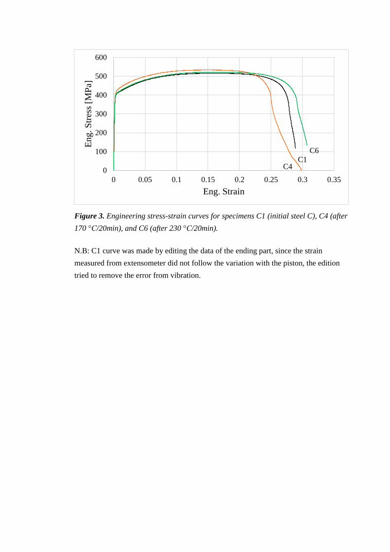
Figure 3. Engineering stress-strain curves for specimens C1 (initial steel C), C4 (after
170 °C/20min), and C6 (after 230 °C/20min).
N.B: C1 curve was made by editing the data of the ending part, since the strain
measured from extensometer did not follow the variation with the piston, the edition
tried to remove the error from vibration.
0
100
200
300
400
500
600
0 0.05 0.1 0.15 0.2 0.25 0.3 0.35
En
g. S
tres
s [M
Pa]
Eng. Strain
C1C4
C6

Appendix C: Representative Engineering Stress-strain Curves
Describing the Effects of Pre-straining and Bake Hardening Heat
Treatments
Figure 1. Engineering stress-strain curves for specimens A4 (170 °C/20min), A8 (2%
pre-strain, 170 °C/20min), A12 (6% pre-strain, 170 °C/20min), A15 (10% pre-strain,
170 °C/20min).
Figure 2. Engineering stress-strain curves for specimens A6 (230 °C/20min), A10 (2%
pre-strain, 230 °C/20min), A14 (6% pre-strain, 230 °C/20min), A18 (10% pre-strain,
230 °C/20min).
0
50
100
150
200
250
300
350
400
450
0 0.05 0.1 0.15 0.2 0.25 0.3 0.35 0.4
En
g. S
tres
s [M
Pa]
Eng. Strain
A4A8
A12
A15
0
50
100
150
200
250
300
350
400
450
0 0.05 0.1 0.15 0.2 0.25 0.3 0.35
En
g. S
tres
s [M
Pa]
Eng. Strain
A6
A10
A14 A1
8

Figure 3. Engineering stress-strain curves for specimens B1 (170℃/20min), B8 (2%
pre-strain, 170 °C/20min), B11 (6% pre-strain, 170 °C/20min), B16 (10% pre-strain,
170°C/20min).
Figure 4. Engineering stress-strain curves for specimens B4 (230 °C/20min), B9 (2%
pre-strain, 230 °C/20min), B13 (6% pre-strain, 230 °C/20min), B17 (10% pre-strain,
230 °C/20min).
0
50
100
150
200
250
300
350
400
450
0 0.05 0.1 0.15 0.2 0.25 0.3 0.35 0.4
En
g. S
tres
s [M
Pa]
Eng. Strain
B1
0
50
100
150
200
250
300
350
400
450
0 0.05 0.1 0.15 0.2 0.25 0.3 0.35 0.4
En
g. S
tres
s [M
Pa]
Eng. Strain
B4
B8 B11
B16
B9
B13
B17

Figure 5. Engineering stress-strain curves for specimens C4 (170 °C/20min), C8 (2%
pre-strain, 170 °C/20min), C12 (6% pre-strain, 170 °C/20min), C16 (10% pre-strain,
170 °C/20min).
Figure 6. Engineering stress-strain curves for specimens C6 (230 °C/20min), C9 (2%
pre-strain, 230 °C/20min), C13 (6% pre-strain, 230 °C/20min), C18 (10% pre-strain,
230 °C/20min).
0
100
200
300
400
500
600
0 0.05 0.1 0.15 0.2 0.25 0.3
En
g. S
tres
s [M
Pa]
Eng. Strain
C4
0
100
200
300
400
500
600
0 0.05 0.1 0.15 0.2 0.25 0.3 0.35
En
g. S
tres
s [M
Pa]
Eng. Strain
C6
C8
C12 C16
C9
C13 C18

Appendix D: Bake Hardening Indexes of Investigated Steels
BH Indexes of Steel A
Heat
Treatment
BH Specimens BH Index
1 (MPa)
Specimens BH Index
2 (MPa)
Average
BH Index
(MPa)
170℃
/20min
BH0 A1-A3 19.1 A1-A4 21.4 20
BH2 A7 39.6 A8 44.0 42
BH6 A11 47.4 A12 48.9 48
BH10 A15 54.4 A16 55.3 55
230℃
/20min
BH0 A1-A5 73.0 A1-A6 73.8 73
BH2 A9 69.5 A10 68.7 69
BH6 A13 65.0 A14 67.9 66
BH10 A17 50.6 A18 61.5 56
BH Indexes of Steel B
Heat
Treatment
BH Specimens BH Index
1 (MPa)
Specimens BH Index
2 (MPa)
Average
BH Index
(MPa)
170℃
/20min
BH0 B6-B1 23.8 B6-B2 11.3 18
BH2 B7 38.0 B8 38.7 38
BH6 B11 42.7 B12 41.7 42
BH10 B15 52.8 B16 54.2 54
230℃
/20min
BH0 B6-B3 68.0 B6-B4 71.5 70
BH2 B9 74.5 B10 72.4 73
BH6 B13 58.6 B14 58.0 58
BH10 B17 63.5 B18 58.0 61

BH Indexes of Steel C
Heat
Treatment
BH Specimens BH Index
1 (MPa)
Specimens BH Index
2 (MPa)
Average
BH Index
(MPa)
170℃
/20min
BH0 C1-C3 38.8 C1-C4 12.8 26
BH2 C7 15.2 C8 15.1 15
BH6 C11 15.5 C12 16.0 16
BH10 C15 26.0 C16 26.3 26
230℃
/20min
BH0 C1-C5 16.2 C1-C6 0.2 8
BH2 C9 21.1 C10 20.2 21
BH6 C13 26.8 C14 26.5 27
BH10 C17 32.3 C18 32.7 33
N.B: Since there are two repeated tests in each case, BH index 1 and 2 are for two tested
results, and their average value is taken as the BH index of the steel.

Appendix E: Representative Engineering Stress-strain Curves of
the Specimens Before and After Aging Treatment
Figure 1. Comparison of the engineering stress-strain curves for steel A before (A1)
and after (AI-A2) 100 °C/30min aging treatment.
Figure 2. Comparison of the engineering stress-strain curves for steel B before (B6)
and after (AI-B1) 100 °C/30min aging treatment.
0
50
100
150
200
250
300
350
400
0 0.05 0.1 0.15 0.2 0.25 0.3 0.35 0.4
En
g. S
tres
s [M
Pa]
Eng. Strain
A1
AI-A2
0
50
100
150
200
250
300
350
400
0 0.05 0.1 0.15 0.2 0.25 0.3 0.35 0.4
En
g. S
tres
s [M
Pa]
Eng. Strain
AI-B1
B6

Figure 3. Comparison of the engineering stress-strain curves for steel C before (C1)
and after (AI-C1) 100 °C/30min aging treatment.
0
100
200
300
400
500
600
0 0.05 0.1 0.15 0.2 0.25 0.3
En
g. S
tres
s [M
Pa]
Eng. Strain
AI-C1
C1