Embed Size (px)
Citation preview

Zentrum fur TechnomathematikFachbereich 3 – Mathematik und Informatik
A level set toolbox includingreinitialization and mass correction
algorithms for FEniCS
Mischa Jahn Timo Klock
Report 16–01
Berichte aus der Technomathematik
Report 16–01 February 2016


A LEVEL SET TOOLBOX INCLUDING REINITIALIZATION
AND MASS CORRECTION ALGORITHMS FOR FENICS
M. JAHN AND T. KLOCK
Abstract. In this article, an overview of the level set method is given and atoolbox for the numerical solution of level set problems is presented. Mainly
based on the work of [8], we mention various aspects of the level set method
including discretization and stabilization aspects, as well as the reinitializa-tion of the level set function. Additionally, global and local mass resp. volume
correction approaches adapted from [8] respectively [16] are presented for main-
taining the level set function during its evolution in time. All described modelsand methods are implemented into a toolbox for the FEniCS framework [14].
1. Introduction
Many engineering processes include time dependent movements of discontinu-ities, e.g. a solid-liquid interface in melting and solidification processes or a surfacewithin a two-phase flow. For the modeling and simulation of such a process, arepresentation of the discontinuity is needed.
There are many approaches available to characterize discontinuities mathemat-ically, however, a very popular choice is the level set method introduced by Osherand Sethian [19]. The basic idea of the level set method is to represent a time de-pendent discontinuity implicitly by the zero level set of a continuous scalar functionwhose evolution in time is described by a transport equation.
Unfortunately, solving the level set equation numerically using standard finiteelements may cause degeneration of the function’s gradient and lack of mass resp.volume conservation. Therefore, a need for methods preserving these propertiesarises, i.e. the level set function has to be reinitialized and the mass resp. volumeenclosed by a level set has to be corrected. In connection with maintaining thefunction, the construction of a discrete representation of the discontinuity has tobe considered.
In this article, a level set toolbox including reinitialization and mass conservingmethods for the finite element framework FEniCS [14] is presented. Started in2003, the idea of the FEniCS Project is to automate the solution of mathematicalmodels based on PDEs. By using different software libraries that are integratedinto one package, the user can specify a PDE-based problem in weak form andFEniCS generates the code automatically. Using this automated code generationapproach, the numerical simulation of different physical processes and engineeringapplications can be easily implemented.
This article is organized as the following: In Section 2, a short introduction tothe level set method including comments on the derivation of the weak formulationof the level set problem is given. Section 3 deals with the discretization and sta-bilization of the level set equation. Following [8], a discrete representation of thediscontinuity is derived and a reinitialization technique is presented. To conservemass during the evolution of the level set function, the approaches of global [8] andlocal [16] mass resp. volume correction are presented. Aspects of the implementa-tion of the level set toolbox in FEniCS are given in detail in Section 4 and numericalresults are shown in Section 5.
1

2 M. JAHN AND T. KLOCK
a) b)
Figure 2.1. Visualization of the idea of the level sets method us-ing a scalar function ϕ: a) Domains Ω+(t) and Ω−(t) are separatedby the zero level set Γ(t) of ϕ. b) Visualization of some level setsof ϕ.
2. The level set method: Review
2.1. Background. The basic idea of the level set method is to define a continuousscalar function ϕ : Ω × [t0, tf ] → R on a given domain Ω ⊂ Rd, d = 2, 3, whereasthe zero level set of ϕ
Γ(t) = x ∈ Ω : ϕ(x, t) = 0, t ∈ [t0, tf ],
represents a time dependent discontinuity, for example an interface, in an implicitway. By using the sign of ϕ = ϕ(·, t), the hold-all domain Ω can be divided intothe subdomains
Ω(t) = Ω+(t) ∪ Ω−(t) ∪ Γ(t),
with x ∈ Ω+(t) ⇔ ϕ(x, t) > 0 and x ∈ Ω−(t) ⇔ ϕ(x, t) < 0. An exemplary sketchof a 2D situation where a hold-all domain Ω is divided by the sign of the functionϕ into subdomains Ω+(t) resp. Ω−(t) is given in Fig. 2.1a and some level sets of ϕare indicated in Fig. 2.1b.
In regards to geometrical properties, the level set method allows for an easycomputation of the normal ~n to Γ
~n =∇ϕ||∇ϕ||
,
and the curvature of Γ reads as
κ = −div~n = −div∇ϕ||∇ϕ||
.
These properties are useful in many applications, e.g. if considering two-phase flowincluding surface tension on the interface or the two-phase Stefan problem.
There are various functions ϕ which can be defined and used within the level setmethod, however, from a numerical point of view it is important, e.g. for a stablecomputation of ~n and κ, that the gradient ||∇ϕ|| does neither vanish nor becometoo big. Due to this, literature suggest to use a so called signed distance function,i.e.
ϕ(x, t) =
− miny∈Γ(t)
||x− y||2, if x ∈ Ω−(t)
miny∈Γ(t)
||x− y||2, if x ∈ Ω+(t),
which satisfies ||∇ϕ|| = 1. This condition is important from a numerical point ofview, as it guarantees a stable computation of ~n and κ.
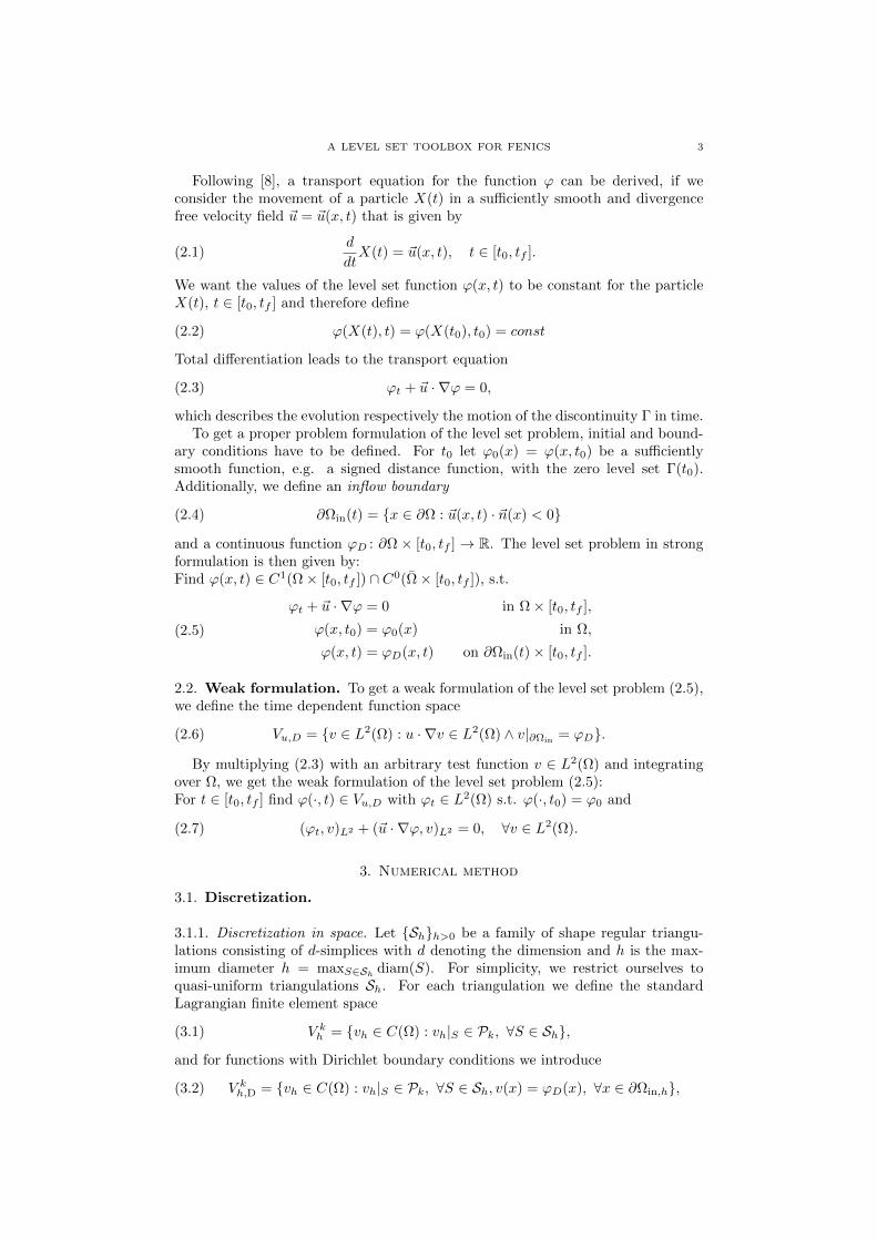
A LEVEL SET TOOLBOX FOR FENICS 3
Following [8], a transport equation for the function ϕ can be derived, if weconsider the movement of a particle X(t) in a sufficiently smooth and divergencefree velocity field ~u = ~u(x, t) that is given by
d
dtX(t) = ~u(x, t), t ∈ [t0, tf ].(2.1)
We want the values of the level set function ϕ(x, t) to be constant for the particleX(t), t ∈ [t0, tf ] and therefore define
ϕ(X(t), t) = ϕ(X(t0), t0) = const(2.2)
Total differentiation leads to the transport equation
ϕt + ~u · ∇ϕ = 0,(2.3)
which describes the evolution respectively the motion of the discontinuity Γ in time.To get a proper problem formulation of the level set problem, initial and bound-
ary conditions have to be defined. For t0 let ϕ0(x) = ϕ(x, t0) be a sufficientlysmooth function, e.g. a signed distance function, with the zero level set Γ(t0).Additionally, we define an inflow boundary
∂Ωin(t) = x ∈ ∂Ω : ~u(x, t) · ~n(x) < 0(2.4)
and a continuous function ϕD : ∂Ω × [t0, tf ] → R. The level set problem in strongformulation is then given by:Find ϕ(x, t) ∈ C1(Ω× [t0, tf ]) ∩ C0(Ω× [t0, tf ]), s.t.
(2.5)
ϕt + ~u · ∇ϕ = 0 in Ω× [t0, tf ],
ϕ(x, t0) = ϕ0(x) in Ω,
ϕ(x, t) = ϕD(x, t) on ∂Ωin(t)× [t0, tf ].
2.2. Weak formulation. To get a weak formulation of the level set problem (2.5),we define the time dependent function space
Vu,D = v ∈ L2(Ω) : u · ∇v ∈ L2(Ω) ∧ v|∂Ωin= ϕD.(2.6)
By multiplying (2.3) with an arbitrary test function v ∈ L2(Ω) and integratingover Ω, we get the weak formulation of the level set problem (2.5):For t ∈ [t0, tf ] find ϕ(·, t) ∈ Vu,D with ϕt ∈ L2(Ω) s.t. ϕ(·, t0) = ϕ0 and
(ϕt, v)L2 + (~u · ∇ϕ, v)L2 = 0, ∀v ∈ L2(Ω).(2.7)
3. Numerical method
3.1. Discretization.
3.1.1. Discretization in space. Let Shh>0 be a family of shape regular triangu-lations consisting of d-simplices with d denoting the dimension and h is the max-imum diameter h = maxS∈Sh diam(S). For simplicity, we restrict ourselves toquasi-uniform triangulations Sh. For each triangulation we define the standardLagrangian finite element space
V kh = vh ∈ C(Ω) : vh|S ∈ Pk, ∀S ∈ Sh,(3.1)
and for functions with Dirichlet boundary conditions we introduce
V kh,D = vh ∈ C(Ω) : vh|S ∈ Pk, ∀S ∈ Sh, v(x) = ϕD(x), ∀x ∈ ∂Ωin,h,(3.2)
4 M. JAHN AND T. KLOCK
with k ≥ 1 and ∂Ωin,h being the discrete influx boundary. Using this functionspaces, (2.7) discretized in space reads: For t ∈ [t0, tf ] find ϕ(·, t) ∈ V kh,D with
~u · ∇ϕh ∈ L2(Ω) such that∑S∈Sh
(∂ϕh∂t
+ ~u · ∇ϕh, vh)L2(S)
= 0, ∀vh ∈ Vh.(3.3)
In many applications, e.g. multi-phase flow, the polynomial degree k = 2 is cho-sen for the finite-dimensional function space (3.2). This is due to different reasons,for example the quality of the curvature approximation of the level set functioncontaining second derivatives, as pointed out in [8]. Moreover, using quadratic ba-sis functions has the additional advantage that the degrees of freedom coincide thethe degrees of freedom of linear basis functions on a regularly refined mesh. Thiswill be extensively exploited for characterizing the interface Γ discretely and by thereinitialization technique.
3.1.2. Discretization in time. For time discretization, a θ−scheme is used here. Wediscretize the interval [t0, tf ] by N + 1 time steps tn = t0 +n∆t, n = 0, . . . , N with∆t denoting the time step. Let θ ∈ [0, 1] be a parameter and ϕnh(·) ≈ ϕ(·, tn) be anapproximation of the level set function ϕ at time tn. The completely discretizedlevel set problem reads∑
S∈Sh
(ϕn+1h − ϕnh
∆t+ θ~un+1∇ϕn+1
h + (1− θ)~un∇ϕnh, vh)L2(S)
= 0,(3.4)
for all vh ∈ Vh. Note that θ = 0 leads to the explicit Euler-scheme while θ = 1results in the implicit Euler-scheme.
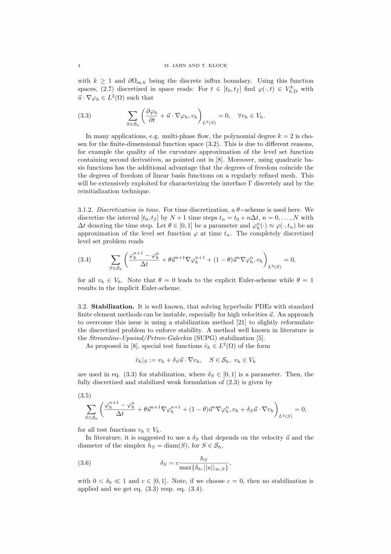
3.2. Stabilization. It is well known, that solving hyperbolic PDEs with standardfinite element methods can be instable, especially for high velocities ~u. An approachto overcome this issue is using a stabilization method [21] to slightly reformulatethe discretized problem to enforce stability. A method well known in literature isthe Streamline-Upwind/Petrov-Galerkin (SUPG) stabilization [5].
As proposed in [8], special test functions vh ∈ L2(Ω) of the form
vh|S := vh + δS~u · ∇vh, S ∈ Sh, vh ∈ Vh
are used in eq. (3.3) for stabilization, where δS ∈ [0, 1] is a parameter. Then, thefully discretized and stabilized weak formulation of (2.3) is given by
∑S∈Sh
(ϕn+1h − ϕnh
∆t+ θ~un+1∇ϕn+1
h + (1− θ)~un∇ϕnh, vh + δS~u · ∇vh)L2(S)
= 0,
(3.5)
for all test functions vh ∈ Vh.In literature, it is suggested to use a δS that depends on the velocity ~u and the
diameter of the simplex hS = diam(S), for S ∈ Sh,
δS = chS
maxδ0, ||u||∞,S,(3.6)
with 0 < δ0 1 and c ∈ [0, 1]. Note, if we choose c = 0, then no stabilization isapplied and we get eq. (3.3) resp. eq. (3.4).
A LEVEL SET TOOLBOX FOR FENICS 5
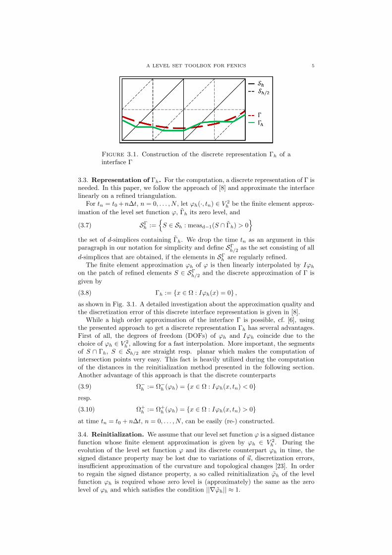
Figure 3.1. Construction of the discrete representation Γh of ainterface Γ
3.3. Representation of Γh. For the computation, a discrete representation of Γ isneeded. In this paper, we follow the approach of [8] and approximate the interfacelinearly on a refined triangulation.
For tn = t0 +n∆t, n = 0, . . . , N , let ϕh(·, tn) ∈ V 2h be the finite element approx-
imation of the level set function ϕ, Γh its zero level, and
SΓh :=
S ∈ Sh : measd−1(S ∩ Γh) > 0
(3.7)
the set of d-simplices containing Γh. We drop the time tn as an argument in thisparagraph in our notation for simplicity and define SΓ
h/2 as the set consisting of all
d-simplices that are obtained, if the elements in SΓh are regularly refined.
The finite element approximation ϕh of ϕ is then linearly interpolated by Iϕhon the patch of refined elements S ∈ SΓ
h/2 and the discrete approximation of Γ is
given by
Γh := x ∈ Ω : Iϕh(x) = 0 ,(3.8)
as shown in Fig. 3.1. A detailed investigation about the approximation quality andthe discretization error of this discrete interface representation is given in [8].
While a high order approximation of the interface Γ is possible, cf. [6], usingthe presented approach to get a discrete representation Γh has several advantages.First of all, the degrees of freedom (DOFs) of ϕh and Iϕh coincide due to thechoice of ϕh ∈ V 2
h , allowing for a fast interpolation. More important, the segmentsof S ∩ Γh, S ∈ Sh/2 are straight resp. planar which makes the computation ofintersection points very easy. This fact is heavily utilized during the computationof the distances in the reinitialization method presented in the following section.Another advantage of this approach is that the discrete counterparts
Ω−h := Ω−h (ϕh) = x ∈ Ω : Iϕh(x, tn) < 0(3.9)
resp.
Ω+h := Ω+
h (ϕh) = x ∈ Ω : Iϕh(x, tn) > 0(3.10)
at time tn = t0 + n∆t, n = 0, . . . , N , can be easily (re-) constructed.
3.4. Reinitialization. We assume that our level set function ϕ is a signed distancefunction whose finite element approximation is given by ϕh ∈ V 2
h . During theevolution of the level set function ϕ and its discrete counterpart ϕh in time, thesigned distance property may be lost due to variations of ~u, discretization errors,insufficient approximation of the curvature and topological changes [23]. In orderto regain the signed distance property, a so called reinitialization ϕh of the levelfunction ϕh is required whose zero level is (approximately) the same as the zerolevel of ϕh and which satisfies the condition ||∇ϕh|| ≈ 1.
6 M. JAHN AND T. KLOCK
There are many reinitialization methods known in literature [10], however, inthis article, we cite the variant of [8] of the Fast Marching Method [22], which isonly applicable to linear functions.
3.4.1. Fast Marching Method. Given a triangulation Sh and a level set functionϕh ∈ V 2
h , we compute the linear interpolation Iϕh of ϕh on the regularly refinedtriangulation Sh/2, cf. Section 3.3. Let D(S) denote the set of degrees of freedom(DOFs) that are given on a simplex S ∈ Sh/2 and D := D(Sh/2) is the (discrete)set of all DOFs on the discretized domain.
The patch of elements related to a DOF v ∈ D(S), S ∈ Sh/2 is given by
P(v) := S ∈ Sh/2 : v ∈ D(S)(3.11)
and the set of (direct) neighbors to v ∈ D(S), i.e. all w ∈ D that are connected tov via an edge of a d-simplex, is defined by
DP(v) =
⋃S∈P(v)
D(S)
\ v.(3.12)
Please note that since we have linear basis functions, the degrees of freedomwithin an element S ∈ Sh/2 can be identified with its vertices. Therefore, wesimplify the notation and use both meanings synonymously.
Initialization phase: Firstly, all degrees of freedom resp. vertices of intersectedelements are considered, i.e. v ∈ DΓ := v ∈ D(S) : S ∈ SΓ
h/2, where SΓh/2
denotes the d-simplices containing the interface Γh, cf. equation (3.7). A geo-metrical approach and standard linear algebra are used to compute the distancebetween v ∈ D(S) ⊂ DΓ and the straight (2D) resp. planar (3D) interface segmentsΓh,S = S ∩ Γh. The computed distances are then used to set the values of adistance function d : DΓ → R. This function d is now extended to the remainingDOFs resp. vertices v ∈ D \ DΓ in an iteration phase.
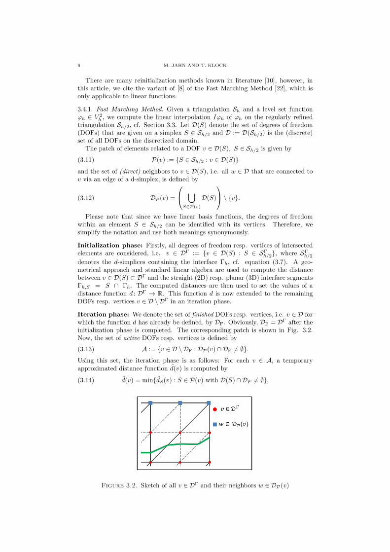
Iteration phase: We denote the set of finished DOFs resp. vertices, i.e. v ∈ D forwhich the function d has already be defined, by DF. Obviously, DF = DΓ after theinitialization phase is completed. The corresponding patch is shown in Fig. 3.2.Now, the set of active DOFs resp. vertices is defined by
A := v ∈ D \ DF : DP(v) ∩ DF 6= ∅.(3.13)
Using this set, the iteration phase is as follows: For each v ∈ A, a temporaryapproximated distance function d(v) is computed by
(3.14) d(v) = mindS(v) : S ∈ P(v) with D(S) ∩ DF 6= ∅,
Figure 3.2. Sketch of all v ∈ DΓ and their neighbors w ∈ DP(v)

A LEVEL SET TOOLBOX FOR FENICS 7
where the value dS(v) is calculated by
(3.15) dS(v) =
d(w) + ‖v − w‖, for D(S) ∩ DF = w,d(PW (v)) + ‖v − PW v‖, for D(S) ∩ DF = wi, i = 2 or 3
with PW as the orthogonal projection of v on the line W := conv(w1, w2) resp. onthe triangle W := conv(w1, w2, w3) for D(S)∩DF = w1, w2 resp. D(S)∩DF =w1, w2, w3. The value d(PW (v)) is therefore interpolated from the alreadycalculated values d(wi) by using the barycentric coordinates of PW (v) on the lineand triangle, respectively.
Afterwards, the DOF resp. vertex v0 ∈ A with
d(v0) = minv∈A
d(v)(3.16)
is added to the finalized set DF and the active set A, the patches P(v), v ∈ D aswell as the set of direct neighbors DP(v) are updated accordingly. Furthermore,
the temporary function d(v) has to be re-computed for the new setting. This loopis performed until A = ∅.
After completing the iteration phase, the (linear) distance function d(v) ≈ |Iϕh|is defined for all v ∈ D and a reinitialized linear level set function, approximating asigned distance function on Sh/2 , is given by Iϕh := d · sign(Iϕh). Using the valuesof the function, a piecewise quadratic function ϕh is then defined on Sh, which isour new reinitialized level set function.
In practice, it turns out that this variant of the Fast Marching Method is morestable and leads to better results, if we do not use the patch P(v) but the extendedpatch Pext(v) considering also all second neighbor cells S of v in eq. (3.14) and eq.(3.15).
3.5. Mass conservation. For a divergence-free velocity field ~u(x, t), the mass ineach subdomain Ω+(t) and Ω−(t) is conserved for all t ∈ [t0, tf ] from an analyticalpoint of view. However, this is not necessarily true for the discretized subdomainsΩ−h (tn) resp. Ω+
h (tn), tn = t0 +n∆t, n = 0, . . . , N , that are obtained by solving thediscretized level set problem in stabilized form using the discrete representation ofΓh, cf. Section 3.3.
As analyzed in [20], the loss of mass will decrease only with decreasing meshsize h and for smaller time steps ∆t since ϕh and resp. Iϕh converges to ϕ. Sincereinitialization methods as the one presented 3.4 are also not mass conserving, anapproach to enforce this property is advisable. For simplicity, we here assumethat no phase transitions occur and that the subdomains separated by the level setfunction do not mix. Thus, the mass of each phase should be constant. Moreover, byusing the notation old resp. new, we indicate that Iϕold
h and Iϕnewh can be the level
set function at different time steps or the functions before and after reinitialization.Due to this, the time as argument is dropped as in the sections before.
We adapt two mass conserving strategies, which are based on a global and alocal consideration of elements. Both mass correction methods take advantage ofthe signed distance property of the level set function by shifting the zero level setusing a function ψh(·, t) ∈ V 1
h/2 such that1
∆V −h = V −h (Iϕoldh )− V −h (Iϕh) = 0(3.17)
holds, with
Iϕh := Iϕnewh + ψh(3.18)
1Instead of V −h (Iϕold
h ) we could also write V −h (Iϕ(·, t0) due to our simplifying assumptions
that no phase transitions occurs and the subdomains do not mix.

8 M. JAHN AND T. KLOCK
and V −h (φ) is defined for a φh ∈ V kh/2 by
V −h (φh) := V −h (φh(·, t)) =
∫x∈Ω:φh(x,t)<0
1dV, t ∈ [t0, tf ].(3.19)
Please note that if (3.17) is true, the same applies to ∆V +h since we have
V +h (Iϕh) = Vh − V −h (Iϕh).(3.20)
Equation (3.17) describes a non-linear problem which has to be solved by aniterative approach. From a numerical point of view, it is important to computethe solution using as few iteration steps and function evaluations as possible. Inthis paper, we use the Anderson/Bjorck variant [3] of the regula falsi method, seeSection 4.3.3 for details.
In the following paragraphs, we describe the mass correction methods for thereinitialization step. Therefore, we can omit the time variable. Please note thatcorrecting the mass defect resulting from time evolution (and without reinitializa-tion) can easily be adapted.
3.5.1. Global approach for mass conservation. A simple approach for correcting themass defect is based on using a globally constant function ψh := ψconst
h ∈ P0(Ωh),ψconsth (x) = ε, ∀x ∈ Ωh in (3.17). Thereby, the value ε can be obtained by finding
the root of the non-linear equation
Z(ε) := V −h (Iϕoldh (·))− V −h (Iϕnew
h (·) + ε) = 0(3.21)
by using the previously mentioned regula falsi method.Due to the fact that the level set function is shifted globally by ε, the corre-
sponding function ψconsth can be added to Iϕnew. Furthermore, this method is
independent from a reinitialization process and does not alter the gradient. There-fore, if using a reinitialization technique, the mass correction can be computed afterthe level set function is reinitialized.
3.5.2. Local approach for mass conservation. A more complex method to conservemass in the level set method, also utilizing the signed distance property, is adaptedfrom [16]. In contrast to the global method, this approach is based on consideringthe mass defects on all elements S ∈ SΓ
h/2, i.e. all elements intersected by Γh,
individually. For these elements, the non-linear equation
ZS(εS) : = V −h,S(Iϕoldh (·))− V −h,S(Iϕnew
h (·) + εS) = 0,(3.22)
with
V −h,S(Iϕh) =
∫Ω−
h ∩S1dV,(3.23)
is solved using the same Anderson/Bjorck variant of the regula falsi method asin the global mass conservation approach. Using the values εS ∈ R, a piecewiseconstant function ψh ∈ P0(S), S ∈ SΓ
h/2, that is discontinuous across element
boundaries is defined by ψh(S) = εS .
Since ψh(S) is a discontinuous function, we cannot add ψh to the level set func-
tion Iϕnewh . Instead, we first define a function
˜ψh ∈ V 1
h/2, cf. (3.2), that is piecewise
linear on S ∈ SΓh/2 and continuous on Ωh. For this purpose, we compute the average
µ of the correction value εS of each DOF v ∈ DΓ by
µ(v) =1
|S ∈ PΓ(v)|∑
S∈PΓ(v)
εS ,(3.24)
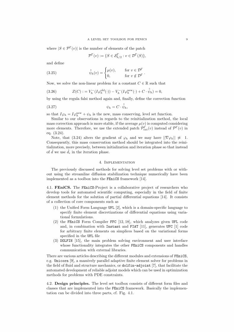
A LEVEL SET TOOLBOX FOR FENICS 9
where |S ∈ PΓ(v)| is the number of elements of the patch
PΓ(v) := S ∈ SΓh/2 : v ∈ DΓ(S),
and define
˜ψh(v) =
µ(v), for v ∈ DΓ
0, for v /∈ DΓ.(3.25)
Now, we solve the non-linear problem for a constant C ∈ R such that
Z(C) : = V −h (Iϕoldh (·))− V −h (Iϕnew
h (·) + C · ˜ψh) = 0,(3.26)
by using the regula falsi method again and, finally, define the correction function
ψh = C · ˜ψh,(3.27)
so that Iϕh = Iϕnewh + ψh is the new, mass conserving, level set function.
Similar to our observations in regards to the reinitialization method, the localmass correction approach is more stable, if the average µ(v) is computed consideringmore elements. Therefore, we use the extended patch PΓ
ext(v) instead of PΓ(v) ineq. (3.24).
Note, that (3.24) alters the gradient of ϕh and we may have ||∇ϕh|| 6≈ 1.Consequently, this mass conservation method should be integrated into the reini-tialization, more precisely, between initialization and iteration phase so that instead
of d we use dε in the iteration phase.
4. Implementation
The previously discussed methods for solving level set problems with or with-out using the streamline diffusion stabilization technique numerically have beenimplemented as a toolbox into the FEniCS framework [14].
4.1. FEniCS. The FEniCS-Project is a collaborative project of researchers whodevelop tools for automated scientific computing, especially in the field of finiteelement methods for the solution of partial differential equations [14]. It consistsof a collection of core components such as
(1) the Unified Form Language UFL [2], which is a domain-specific language tospecify finite element discretizations of differential equations using varia-tional formulations.
(2) the FEniCS Form Compiler FFC [12, 18], which analyzes given UFL codeand, in combination with Instant and FIAT [11], generates UFC [1] codefor arbitrary finite elements on simplices based on the variational formsspecified in the UFL file
(3) DOLFIN [15], the main problem solving environment and user interfacewhose functionality integrates the other FEniCS components and handlescommunication with external libraries.
There are various articles describing the different modules and extensions of FEniCS,e.g. Unicorn [9], a massively parallel adaptive finite element solver for problems inthe field of fluid and structure mechanics, or dolfin-adjoint [7], that facilitate theautomated development of reliable adjoint models which can be used in optimizationmethods for problems with PDE constraints.
4.2. Design principles. The level set toolbox consists of different form files andclasses that are implemented into the FEniCS framework. Basically the implemen-tation can be divided into three parts, cf. Fig. 4.1.

10 M. JAHN AND T. KLOCK
Figure 4.1. Implementation structure: Form (header) files, ob-ject classes and utility functions
Form files. Using the UFL syntax, the stabilized level set problem2, cf. eq. (3.5),is formulated in the files LevelSetEquation2D.ufl and LevelSetEquation3D.ufl
for two resp. three dimensions. After running the FFC compiler on these files, thecorresponding C++ header files are automatically generated, containing most ofthe problem specific data and therefore being the basis to solving the transportequation.
Object class. The classes LevelSetCalculator2D and LevelSetCalculator3D con-tain dimension depending constructors that create the object and routines for solv-ing the transport equation named updateLevelSetFunction. Therefore, the previ-ously mentioned Form files are included providing the level set specific background,e.g. the bilinear form a and the linear form L. Furthermore, the basics of there-distancing method are implemented here, which rely mostly on dimension in-dependent algorithms that are specified in the LevelSetCalculatorUtils. Dueto their dimension dependence, the reinitialization and mass conservation are in-tegrated in the update-routine. Parameters like the frequency of reinitializing thelevel set function are passed to the methods using a list. The default variant isto perform a reinitialization step and the local mass conservation procedure afterevery time step.
Utility class. Aside from the automatically generated problem header files, mostimplementation aspects are covered in the utility class LevelSetCalculatorUtilswhich consists of various static methods, i.e. methods that do not belonging to anyobject. In detail, this class contains a routine implementing the iteration phase ofthe reinitialization approach, mass conservation methods and some helper functions.In this paragraph, we want to present the helper methods briefly:
hasSignSwitchOnCell: A method to check whether the zero level set Γhintersects the cell. It can be easily done by checking for sign switches ofthe level set DOFs corresponding to the cell.build IntersectedNeighborPatch: A method to build the patch consist-ing of the first and second neighbors of any cell (input parameter), whichare intersected by Γh.find PlanarLevelsetSegment: This method is used to calculate the in-tersection points given by the zero level set Γh and the edges of any givencell (input data).determine NodeToLineDistance: This is used to calculate distances be-tween a given point and a finite line, which is given by the endpoints of theline. Additionally it stores the barycentric coordinates to the orthogonalprojection of the vertex on the line.determine NodeToTriangleDistance: Same as above, only with a trian-gle given by three corner points instead of the finite line.
4.3. Level set toolbox. For using the level set toolbox, the user has to createan object of the type LevelSetCalculator2D or LevelSetCalculator3D in his
2Note that by setting δ = 0, the unstabilized problem can be reconstructed.

A LEVEL SET TOOLBOX FOR FENICS 11
Algorithm 1 Using the Levelset Toolbox
[...] // Initialization etc.// Creating and extending the parameters structure: Since all methods are// hidden within the object class, the reinitialization frequency, the volume// correction method etc. are added and defined within the parameters structure.dolfin::Parameters parameters; parameters.add("foo", foo);
// Creating an object of type LevelSetCalculatorXD
LevelSetCalculatorXD lc(mesh, ~u(x, t), ϕh(t0), parameters);
// Update LevelSetCalculatorXD lc object based on the specified parameters.lc.updateLevelSetFunction();[...]
code, depending on the geometrical dimension. This is done by calling the classconstructor with the input data
(1) a triangulation Sh,(2) the (initial) velocity field ~u(x, t),(3) an initial function ϕh ∈ V 2
h ,(4) a parameter list including e.g.. the time stepping scheme, the stabilization
parameter, and the reinitialization method as well as its frequency(5) optional: an influx boundary ∂Ωin(t) and its boundary condition,
as shown in Algorithm 1.
4.3.1. Solving the level set equation. After creating the object, the next evolutionstep of the level set function resp. the surface can be computed by calling theupdateLevelSetFunction member function without any input. The routine usesthe data provided by the object and solves the level set problem with DOLFIN-methods. Due to the fact that the level set function is given by a reference tothe calculator object, the user automatically gets access to the updated level setfunction.
4.3.2. Reinitialization of the level set function. When creating an object of thetype LevelSetCalculator2D resp. LevelSetCalculator3D, the triangulation Shis regularly refined and the piecewise quadratic level set function ϕh is linearlyinterpolated by Iϕh on the generated triangulation Sh/2. Note that the degrees
of freedom of the linear approximation Iϕh coincide with the DOFs of ϕh on SΓh
which allows for a fast and efficient interpolation.For Iϕh, the reinitialization method described in Section 3.4 is separated into an
initialization phase and an iteration phase3. Basically, the implementation of thereinitialization method uses three containers:
(1) DΓ, the set of DOFs belonging to elements S ∈ Sh/2 intersected by theinterface Γh. In the code DΓ is realized as a vector of booleans.
(2) DF , the set of DOFs whose distance to Γh have already been computed.Like DΓ it is realized as a vector of booleans.
(3) A, a set of active DOFs for which a temporary distance d is computed.
For a practical point of view, one has to consider that the initialization phasedepends heavily on the geometrical dimension and, consequently, is implementedas a private function within in the object class. The principal algorithm for the3D situation is shown in Algorithm 2. In contrast to the initialization phase, theiteration phase can be implemented almost independently from the dimension inthe utility class.
3If a local mass conservation algorithm shall be applied, this would be called after the initial-ization phase with the d(v)-values as an input, c.f. 4.3.3.

12 M. JAHN AND T. KLOCK
Algorithm 2 Fast marching method: initialization phase (3D)
Require: Refined mesh Sh/2, linear level set function Iϕh.
Set up containers DF = DΓ (false as default) and d (−1 as default) for the finishedDOFs and the d-values.
Initialize the set DF of finished DOFs:for S ∈ Sh/2 do
if hasSignSwitchOnCell(S) == true thenfor v ∈ D(S) do
Mark DOF v as true in DF .
Calculate the distance to the (linear) zero level set Γh for every v ∈ DF :for v ∈ D do
if DF (v) == true thenBuild the intersected neighbor patch and store the cells in N (by usingbuild IntersectedNeighborPatch).while N 6= do
Take the first cell from N and store it to S. Calculate the intersected zerolevel set Γh(S) and store it into a vector of points called V.if |V| == 2 then
Use determine NodeToLineDistance to calculate the distance of v tothe line given by the two nodes and store it in dtemp.
if |V| == 3 thenUse determine NodeToTriangleDistance to calculate the distance of vto the line given by the two nodes and store it in dtemp.
if |V| == 4 thenSeparate the quadrilateral into two triangles and calculate the distanceto both. Set the smaller one as dtemp.
if d(v) = −1 (default value) or dtemp < d(v) thend(v) = dtemp.
Erase S from the patch N .
return d(v) for every v ∈ DΓ(S), S ∈ SΓh/2.
For the computation of the temporary values d(v), the method called calculate-
DistanceMethod is implemented as shown in Algorithm 3. However, to account forthe permanently changing values d in an efficient way, we save the DOFs, whichare neighbors of the current processed DOF v and only recalculate the d-value forthis DOFs. Every other d-value cannot be influenced by adding v to the finishedset. The re-computation of the whole active set increases the calculation time a lot.Additionally, we want to point out, that a c++ multimap with a double as the keyand a unsigned int as the value is a good way to implement an ordered active setA because the DOF with minimal d-value is always at position 0. The completeiteration phase is presented as pseudo code in Algorithm 4.
4.3.3. Volume/mass conservation. The mass correction methods presented in thispaper take advantage of the signed distance property and are based on the com-putation of the volume of patches of elements. As mentioned in Section 3.5, itis important to use an efficient method to compute the quantities ε in eq. (3.21)resp. εS in (3.22). For both methods this is done by using an advanced regula falsialgorithm that is presented in [3]. The idea of the method is given in Algorithm 5.
Except for this method, the most important routines used in the implemen-tation of the mass correction methods are calculateLevelSetDifference and
A LEVEL SET TOOLBOX FOR FENICS 13
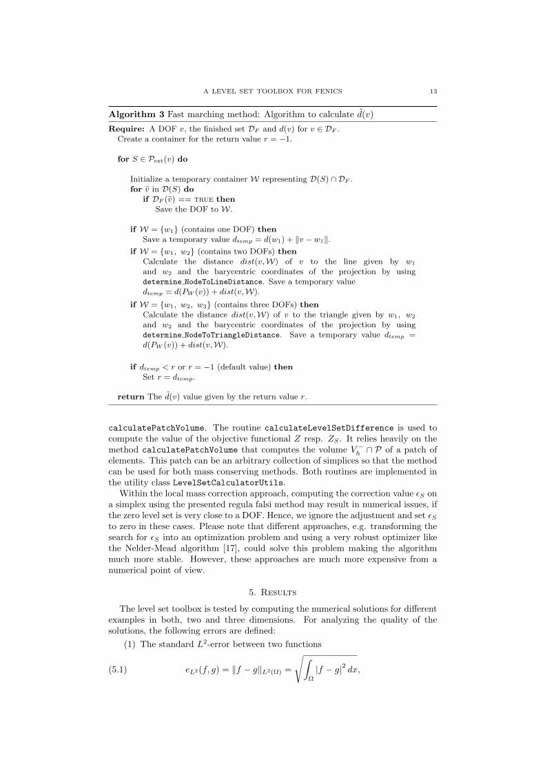
Algorithm 3 Fast marching method: Algorithm to calculate d(v)
Require: A DOF v, the finished set DF and d(v) for v ∈ DF .Create a container for the return value r = −1.
for S ∈ Pext(v) do
Initialize a temporary container W representing D(S) ∩ DF .for v in D(S) do
if DF (v) == true thenSave the DOF to W.
if W = w1 (contains one DOF) thenSave a temporary value dtemp = d(w1) + ‖v − w1‖.
if W = w1, w2 (contains two DOFs) thenCalculate the distance dist(v,W) of v to the line given by w1
and w2 and the barycentric coordinates of the projection by usingdetermine NodeToLineDistance. Save a temporary valuedtemp = d(PW (v)) + dist(v,W).
if W = w1, w2, w3 (contains three DOFs) thenCalculate the distance dist(v,W) of v to the triangle given by w1, w2
and w2 and the barycentric coordinates of the projection by usingdetermine NodeToTriangleDistance. Save a temporary value dtemp =d(PW (v)) + dist(v,W).
if dtemp < r or r = −1 (default value) thenSet r = dtemp.
return The d(v) value given by the return value r.
calculatePatchVolume. The routine calculateLevelSetDifference is used tocompute the value of the objective functional Z resp. ZS . It relies heavily on themethod calculatePatchVolume that computes the volume V −h ∩ P of a patch ofelements. This patch can be an arbitrary collection of simplices so that the methodcan be used for both mass conserving methods. Both routines are implemented inthe utility class LevelSetCalculatorUtils.
Within the local mass correction approach, computing the correction value εS ona simplex using the presented regula falsi method may result in numerical issues, ifthe zero level set is very close to a DOF. Hence, we ignore the adjustment and set εSto zero in these cases. Please note that different approaches, e.g. transforming thesearch for εS into an optimization problem and using a very robust optimizer likethe Nelder-Mead algorithm [17], could solve this problem making the algorithmmuch more stable. However, these approaches are much more expensive from anumerical point of view.
5. Results
The level set toolbox is tested by computing the numerical solutions for differentexamples in both, two and three dimensions. For analyzing the quality of thesolutions, the following errors are defined:
(1) The standard L2-error between two functions
(5.1) eL2(f, g) = ‖f − g‖L2(Ω) =
√∫Ω
|f − g|2 dx,

14 M. JAHN AND T. KLOCK
Algorithm 4 Fast marching method: iteration phase
Require: The finished set Df after the initialization phase and the corresponding d-values.
Initialize the active set A:for every DOF v of the mesh do
if DF (v) is true thenfor every DOF n directly connected to v do
Calculate d(n) by calling calculateDistanceFunction and save it orderedto the active set.
while A is not empty doStore the first DOF of A in v and erase it from A.Set DF (v) to true and d(v) to d(v).Create a boolean container N with false as default to save direct neighbors of v.
for every direct neighbor n of v doif n is not in A nor in DF then
Save n to A and with respect to the correct order by callingcalculateDistanceFunction.
else if n is not in DF thenMark n by adding it to N for the calculation of a possibly new d-value.
for every DOF n of the mesh doif n ∈ N then
Recalculate d(n) by calling calculateDistanceFunction.
if d(n) has changed thenErase n from A and reinsert it to restore the right order.
for every DOF v of the mesh doSet the linearized level set DOF according to Iϕh(v) = sign(ϕh(v))d(v).
Interpolate the linearized level set function Iϕh by the quadratic level set functionϕh by using the one-to-one DOF relation.
return A reinitialized level set function ϕh
Algorithm 5 Regula falsi method in the Anderson/Bjorck variant
Require: The objective function f , left and right initial values z1 and z2.repeat
Calculate fi = f(zi), i ∈ 1, 2.Calculate z = z1 − f1 · (f2 − f1)/(z2 − z1) and fz = f(z).if fz · f2 < 0 then
Set z1 = z2, f1 = f2, z2 = z and f2 = fz.else
Calculate m according to
m =
1− fz/f2 if 1− fz/f2 ≥ 0,
1/2 else.
Set f1 = mf1, z2 = z, f2 = fz and z1 = z1.
until |z1 − z2| < Tolz and |fz| < Tolfz .return An approximation z to the root of f .
(2) the relative volume error between two functions
(5.2) eVol(f, g) =|V −(f)− V −(g)|
V −(f),

A LEVEL SET TOOLBOX FOR FENICS 15
with
V −(f) =
∫x∈Ω:f(x,tn)<0
1dx.
(3) the maximum euclidean distance error between the zero level set Γg of afunction g to the nearest point of the zero level set Γf of a function f
(5.3) e∞(f, g) = maxx2∈Γg
minx1∈Γf
‖x1 − x2‖2.
In the following, the function f will always represent the initial signed distancefunction to a certain shape Ω(0) or a reference solution, respectively, while g willalways be our numerical computed solution ϕh at t = tf . Thereby, it will bementioned, if reinitialization and mass conservation methods are used within thecomputation. Please note that all examples are chosen so that ϕh(·, tf ) shouldcoincide with the original zero level set at t = t0.
5.1. 2D-Example: Deformation flow. On Ω = [0, 1]2 consider a circle centeredat (0.5, 0.75) with a radius of 0.15. The initial level set Γ at t = 0 is given by thesigned distance function ϕ0 to the circle
(5.4) d(x, y) =√
(x− 0.5)2 + (y − 0.75)2 − 0.15
and a time dependent velocity field u(t, x, y) is given by
(5.5) u(t, x, y) =
(− sin2(πx) sin(2πy) cos(πt/tf )
sin(2πx) sin2(πy) cos(πt/tf )
),
with t ∈ [0, 2]. The characteristic of this example, which has been published by [13]and is also considered as a benchmark example in [4], is that during the period0 < t < 1, the circle is deformed and stretched while for 1 < t < 2 a reversal phasetakes place so that at t = 2, the initial shape of a circle is recovered, see Fig. 5.1
Time stepping. Our first test addresses the error introduced by the time discretiza-tion. Here, we consider the implicit Euler scheme, which means θ = 1 in eq. (3.4),and the Crank-Nicolson scheme corresponding to θ = 0.5.
Since we are only interested in errors resulting from time discretization, a coarseuniform mesh with 2 × (10 × 10) elements is chosen. The stabilization parameterδT is time dependent and computed with (3.6) and c = 0.1. Apart from that, noother method, e.g. reinitialization or mass conservation methods are used duringthis test.
Please note that if no stability, reinitialization and mass conservation methodsare used, the numerical solution computed using the Crank-Nicolson time discretiza-tion scheme will be the interpolation of d onto the space V 2
h for t = 2 due to thesymmetry of the example. cf. [8]. This analytical result is reproduced if solving
Figure 5.1. 2D Example deformation flow: Reference solutionϕh(x, t) with ϕh(x, 0) = ϕh(x, 2) at t = 0, t = 0.5, t = 1, t = 1.5and t = 2.

16 M. JAHN AND T. KLOCK
∆t Implicit Euler (θ = 1) Crank-Nicolson (θ = 0.5)20/10 3.25e− 2 6.10e− 3
2−1/10 1.86e− 2 1.54e− 32−2/10 1.01e− 2 3.87e− 42−3/10 5.36e− 3 9.68e− 52−4/10 2.71e− 3 2.42e− 52−5/10 1.32e− 3 5.99e− 62−6/10 5.92e− 4 1.45e− 6
Table 1. L2-errors ‖dref ( 12 tf )−ϕie
h ( 12 tf )‖L2(Ωh) and ‖dref ( 1
2 tf )−ϕcnh ( 1
2 tf )‖L2(Ωh) for different time step sizes on a mesh consistingof 2× 10× 10 = 200 elements.
the example with our level set toolbox 4. Therefore, we use the Crank-Nicolsontime discretization scheme without stabilization, reinitialization or mass conserva-tion methods to compute the reference solution using a very small time step size of∆t = 2−5/100. This reference solution dref (x, t) is then used for the computationof the L2-errors and the analysis of the convergence behavior.
The results in Table 1 show that the solution computed with the toolbox con-verges as one would expect, i.e. it converges linearly, if the implicit Euler schemeis used, and quadratically, if applying the Crank-Nicolson scheme to the problem.Additionally, it can be noted that for a fixed time step size, the overall error whenusing the Crank-Nicolson scheme is smaller compared to the implicit Euler dis-cretization.
Stabilization. As mentioned in Section 3.2, the level set problem often has to bestabilized. On two uniformly constructed meshes with 2 × 40 × 40 = 3200 and2× 80× 80 = 12800 elements consider problem (3.5) with θ = 1, i.e. implicit Eulertime discretization5. Now, we compare the differences in the L2 norm at t = tfbetween our initial signed distance function ϕh(0) = d and the numerical solutionswithout applying stabilization ϕ0
h(tf ) and with factor c = 0.5, i.e. ϕ0.5h (tf ).
As for the constant δ0 of (3.6), we choose δ0 = hS , which is globally constant
given by√
2/40 resp.√
2/80 for the used meshes. Aside from this, no additionalalgorithms like reinitialization or mass conservation are applied for this scenario.
Examining the results which are given in Table 2, one can see that the influenceof an applied stabilization parameter is very small in this scenario6. Therefore, wedo not use this technique for the other examples. However, please note that theinfluence of the stabilization parameter depends highly on the velocity field and theexample.
Reinitialization and mass conservation. The most important aspects of the levelset toolbox are reinitialization and mass conservation. As previously described, thenumerical solution of the level set problem does not preserve the signed distanceproperty and, moreover, lack mass conservation, especially if reinitialization tech-niques are used. Additionally it has to be noted that the L2-error of a reinitializedlevel set function does not converge to zero for finer meshes. This is due to the
4The L2-error between the interpolation of d onto V 2h and the calculated ϕh(t = 2) using the
the Crank-Nicolson scheme is within the range of computational accuracy, i.e. smaller than 10−15.5As mentioned, using the Crank-Nicolson time discretization scheme would only be reasonable
in this scenario for t ∈ [t0,tf2
].6We tested varying the constant c ∈ [0, 2] on several mesh sizes and time step sizes with similar
results

A LEVEL SET TOOLBOX FOR FENICS 17
∆t No stability (c = 0) With stability (c = 0.5)2× 40× 40 2× 80× 80 2× 40× 40 2× 80× 80
0.1 5.02e− 2 4.13e− 2 5.02e− 2 5.02e− 20.05 3.21e− 2 3.21e− 2 3.21e− 2 3.21e− 2
0.025 1.91e− 2 1.91e− 2 1.91e− 2 1.91e− 20.01 9.09e− 3 9.09e− 3 9.11e− 3 9.09e− 3
0.005 5.05e− 3 5.05e− 3 5.10e− 3 5.05e− 30.0025 2.76e− 3 2.76e− 3 2.87e− 3 2.77e− 3
Table 2. Errors ‖ϕh(0) − ϕ0h(tf )‖L2 (without stabilization) and
‖ϕh(0) − ϕ0.5h (tf )‖L2
(with stabilization) with respect to differenttime step and mesh sizes.
fact that the fast marching method only guarantees the property ‖∇ϕh‖ ≈ 1 in aclose range to the zero level set while the reinitialized function differs from the realsigned distance function d in the far field. Therefore, we compare the evol and e∞errors in this section instead of the difference in the L2 norm.
On different meshes with diam h =√
2/32, . . . ,√
2/512, we use the Crank-Nicolson scheme without stabilization, i.e. means θ = 0.5 and δS = 0. The timestep size is ∆t = 0.01 and we will compare the situations where
(1) only reinitialization ( “R“),(2) reinitialization with global mass conservation (called ”RGM“), and(3) reinitialization with local mass conservation (called ”RLM“)
methods are used after every time step, which means that the respective methodis used in every single computation step. All results are presented in Table 3and visualized in Figure 5.2. Exemplary results of all methods on meshes with2× 32× 32 = 2048 and 2× 64× 64 = 8192 elements are given in Figure 5.3.
According to this test scenario, only using a reinitialization technique withoutcorrecting the mass defect gives the worst results, the case where reinitializationand local mass conservation methods are used gives in contrast the smallest errors.If instead of local mass conservation we employ the global strategy, the volumeerrors are still very small. However, the drawback of this rather simple approach isthat the shape of the zero level set Γh is also conserved, i.e. the zero level set doesnot change its shape as it should do according to the velocity field. This leads to ahigher e∞ error.
In brief, our main conclusions regarding reinitialization and mass correction are:Firstly with applied reinitialization, mass conservation should be used as well be-cause the reinitialization has a negative effect on the zero level set reconstruction.
√2/h R RGM RLM
evol[%] e∞ evol[%] e∞ evol[%] e∞32 19.14 3.60e− 2 1.77 2.59e− 2 2.28 7.22e− 364 4.85 1.05e− 2 0.68 8.02e− 3 0.68 2.21e− 3
128 1.32 3.28e− 3 0.26 2.91e− 3 0.255 1.42e− 3256 0.39 1.36e− 3 0.12 1.22e− 3 0.12 9.2e− 4512 0.13 6.55e− 4 6.89e− 2 6.41e− 4 7.26e− 4 5.60e− 4
Table 3. Errors evol(d, ϕh(tf )) and e∞(d, ϕh(tf )) of the reinitial-ization and mass conservation algorithms with respect to h.
18 M. JAHN AND T. KLOCK
a) b)
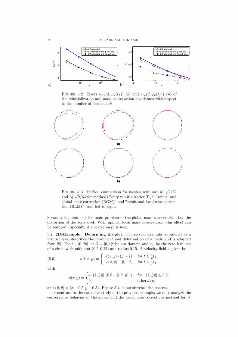
Figure 5.2. Errors evol(d, ϕh(tf )) (a) and e∞(d, ϕh(tf )) (b) ofthe reinitialization and mass conservation algorithms with respectto the number of elements N .
a)
b)
Figure 5.3. Method comparison for meshes with size a)√
2/32
and b)√
2/64 for methods ”only reinitialization(R)“, ”reinit. andglobal mass correction (RGM)“ and ”reinit and local mass correc-tion (RLM)“ from left to right.
Secondly it points out the main problem of the global mass conservation, i.e. thedistortion of the zero level. With applied local mass conservation, this effect canbe reduced, especially if a coarse mesh is used.
5.2. 2D-Example: Deforming droplet. The second example considered as atest scenario describes the movement and deformation of a circle and is adaptedfrom [8]. For t ∈ [0, 20] let Ω = [0, 1]2 be our domain and ϕ0 be the zero level setof a circle with midpoint (0.5, 0.25) and radius 0.15. A velocity field is given by
u(t, x, y) =
c(x, y) · (y,−x), for t ≤ 1
2 tf ,
−c(x, y) · (y,−x), for t > 12 tf ,
(5.6)
with
c(x, y) =
4||(x, y)|| (0.5− ||(x, y)||), for ||(x, y)|| ≤ 0.5,
0, otherwise,
and (x, y) = (x− 0.5, y − 0.5). Figure 5.4 shows sketches the process.In contrast to the extensive study of the previous example, we only analyze the
convergence behavior of the global and the local mass corrections method for N

A LEVEL SET TOOLBOX FOR FENICS 19
Figure 5.4. 2D Example rising deforming droplet: Reference so-lution ϕh(x, t) with ϕh(x, 0) = ϕh(x, 20) at t = 0, t = 5, t = 10,t = 15 and t = 20.
0 0.5 1 1.5 2 2.5 3 3.50
0.1
0.2
0.3
0.4
delta t = 10−x
evol (
%)
N = 512
N = 2048
N = 8192
N = 32768
0 0.5 1 1.5 2 2.5 3 3.50
0.05
0.1
0.15
0.2
delta t = 10−x
evol (
%)
N = 512
N = 2048
N = 8192
N = 32768
Figure 5.5. Errors evol(d, ϕh(tf )) the global (left) and local(right) mass conservation algorithms.
varied between 2×24×24 and 2×27×27 and ∆t = 20, 2−1, ..., 2−5. The convergencebehavior of the L2-errors are visualized is Figure 5.5.
As one can see, the error depends mainly on the spatial discretization. This isto be expected since reinitialization and mass correction is applied after every timestep. Furthermore it can be observed that the error if using the local mass correctionscheme is much smaller compared to the global mass conservation method.
5.3. 3D-Example: Deformation flow. Now, we enhance the example 5.1 andchoose a domain Ω = [0, 1]3 containing a sphere centered at (0.35, 0.35, 0.35) witha radius of 0.15. The initial condition ϕ0 is given by
(5.7) d(x, y, z) =√
(x− 0.35)2 + (y − 0.35)2 + (z − 0.35)2 − 0.15.
and the prescribed velocity field is given by
(5.8) u(t, x, y, z) =
2 sin2(πx) sin(2πy) sin(2πz) cos(πt/tf )− sin(2πx) sin2(πy) sin(2πz) cos(πt/tf )− sin(2πx) sin(2πy) sin2(πz) cos(πt/tf )
where the time span is again given by [t0, tf ] = [0, 2] with a stretching phase untilt = 1 and a reversal phase from 1 to 2. As before, this example, visualized in Figure5.6 has been first published in [13] and used as a benchmark scenario in [4].
Just as in the 2D case, the difference between both mass conservation methodsin the relative error evol is rather small. In fact, for higher mesh resolutions, theerror of the global approach seems to be smaller than for the local conservationscheme. As for the e∞ error, the local mass defect correction approach allows fora much better approximation of the shape. Exemplary results for t = 2 = tf areshown in Figure 5.8.
5.4. 3D-Example: Deforming droplet. The last scenario considered in thispaper extends example 5.2 to three dimensions [8]. Let Ω = [0, 1]3, t ∈ [0, 20] and ϕ0

20 M. JAHN AND T. KLOCK
Figure 5.6. 3D Example deformation flow: Reference solutionϕh(x, t) with ϕh(x, 0) = ϕh(x, 2) at t = 0, t = 0.25, t = 0.5,t = 1.0, t = 1.5 and t = 2.0.
a)10
410
510
610
710
−3
10−2
10−1
100
N
evo
l (%
)
3D with reinit. and gl. vol. corr.
3D with reinit. and loc. vol. corr.
b)10
410
510
610
710
−2
10−1
100
N
evo
lab
s
3D with reinit. and gl. vol. corr.
3D with reinit. and loc. vol. corr.
Figure 5.7. Errors evol(d, ϕh(tf )) (a) and e∞(d, ϕh(tf )) (b) ofthe reinitialization and mass conservation algorithms with respectto the number of elements N .
Figure 5.8. 3D Example deformation flow: Reference solutionand numerical solution for mesh sizes 6 × 24 × 24, 6 × 44 × 44and 6 × 64 × 64 at (t = 2)using reinitialization and local volumecorrection.
be the zero level set of a sphere with radius 0.2 which is centered at (0.5, 0.25, 0.5).The velocity field u(t, x, y, z) is given by
u(t, x, y, z) =
c(x, y, z) · (y,−x, 0), for t ≤ 1
2 tf ,
−c(x, y, z) · (y,−x, 0), for t > 12 tf ,
(5.9)
with
c(x, y, z) =
4||(x, y, z)|| (0.5− ||(x, y, z)||), for ||(x, y, z)|| ≤ 0.5,
0, otherwise,
and (x, y, z) = (x − 0.5, y − 0.5, z − 0.5). The movement and deformation of thedroplet in this example is shown for different times in Figure 5.9.
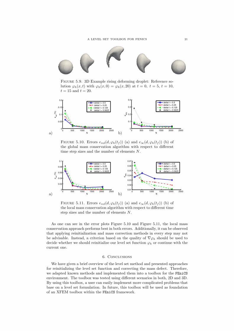
A LEVEL SET TOOLBOX FOR FENICS 21
Figure 5.9. 3D Example rising deforming droplet: Reference so-lution ϕh(x, t) with ϕh(x, 0) = ϕh(x, 20) at t = 0, t = 5, t = 10,t = 15 and t = 20.
a)0 500 1000 1500 2000 2500
0
0.05
0.1
0.15
0.2
N
evo
l (%
)
deltat t = 0.5
deltat t = 0.25
deltat t = 0.125
deltat t = 0.0625
b)0 500 1000 1500 2000 2500
0
0.1
0.2
0.3
0.4
N
ea
bs
deltat t = 0.5
deltat t = 0.25
deltat t = 0.125
deltat t = 0.0625
Figure 5.10. Errors evol(d, ϕh(tf )) (a) and e∞(d, ϕh(tf )) (b) ofthe global mass conservation algorithm with respect to differenttime step sizes and the number of elements N .
a)0 500 1000 1500 2000 2500
0
0.02
0.04
0.06
0.08
0.1
N
evo
l (%
)
deltat t = 0.5
deltat t = 0.25
deltat t = 0.125
deltat t = 0.0625
b)0 500 1000 1500 2000 2500
0.01
0.02
0.03
0.04
0.05
0.06
0.07
N
ea
bs
deltat t = 0.5
deltat t = 0.25
deltat t = 0.125
deltat t = 0.0625
Figure 5.11. Errors evol(d, ϕh(tf )) (a) and e∞(d, ϕh(tf )) (b) ofthe local mass conservation algorithm with respect to different timestep sizes and the number of elements N .
As one can see in the error plots Figure 5.10 and Figure 5.11, the local massconservation approach performs best in both errors. Additionally, it can be observedthat applying reinitialization and mass correction methods in every step may notbe advisable. Instead, a criterion based on the quality of ∇ϕh should be used todecide whether we should reinitialize our level set function ϕh or continue with thecurrent one.
6. Conclusions
We have given a brief overview of the level set method and presented approachesfor reinitializing the level set function and correcting the mass defect. Therefore,we adapted known methods and implemented them into a toolbox for the FEniCS
environment. The toolbox was tested using different scenarios in both, 2D and 3D.By using this toolbox, a user can easily implement more complicated problems thatbase on a level set formulation. In future, this toolbox will be used as foundationof an XFEM toolbox within the FEniCS framework.

22 M. JAHN AND T. KLOCK
Acknowledgement
The authors gratefully acknowledge the financial support by the DFG (GermanResearch Foundation) for the subproject A3 within the Collaborative ResearchCenter SFB 747 “Mikrokaltumformen - Prozesse, Charakterisierung, Optimierung”.

A LEVEL SET TOOLBOX FOR FENICS 23
References
[1] M. S. Alnaes, A. Logg, K.-A. Mardal, O. Skavhaug, and H. P. Langtangen. Unified framework
for finite element assembly. International Journal of Computational Science and Engineering,
4(4):231–244, 2009.[2] M. S. Alnaes, A. Logg, K. B. Olgaard, M. E. Rognes, and G. N. Wells. Unified form lan-
guage: A domain-specific language for weak formulations of partial differential equations.
ACM Trans. Math. Softw., 40(2):9:1–9:37, March 2014.[3] Ned Anderson and Ake Bjorck. A new high order method of regula falsi type for computing
a root of an equation. BIT Numerical Mathematics, 13(3):253–264, 1973.
[4] R. Ausas, E. Dari, and G. Buscaglia. A mass-preserving geometry-based reinitializationmethod for the level set function. Mecanica Computacional, 27:25–27, 2008.
[5] A. N. Brooks and T. J. R. Hughes. Streamline upwind/petrov-galerkin formulations for con-
vection dominated flows with particular emphasis on the incompressible navier-stokes equa-tions. Comput. Methods Appl. Mech. Eng., pages 199–259, 1990.
[6] K. W. Cheng and T.-P. Fries. Higher-order xfem for curved strong and weak discontinuities.International Journal for Numerical Methods in Engineering, 82(5):564–590, 2010.
[7] P. E. Farrell, D. A. Ham, S. W. Funke, and M. E. Rognes. Automated derivation of the ad-
joint of high-level transient finite element programs. SIAM Journal on Scientific Computing,35(4):C369–C393, 2013.
[8] S. Gross and A. Reusken. Numerical Methods for Two-phase Incompressible Flows. Springer
Series in Computational Mathematics. Springer, 2011.[9] J. Hoffman, J. Jansson, C. Degirmenci, N. Jansson, and M. Nazarov. Unicorn: a Unified
Continuum Mechanics Solver, chapter 18. Springer, 2012.
[10] S. Hysing. A new implicit surface tension implementation for interfacial flows. InternationalJournal for Numerical Methods in Fluids, 51(6):659–672, 2006.
[11] R. C. Kirby. Algorithm 839: Fiat, a new paradigm for computing finite element basis func-
tions. ACM Trans. Math. Softw., 30(4):502–516, December 2004.[12] R. C. Kirby and A. Logg. A compiler for variational forms. ACM Trans. Math. Softw.,
32(3):417–444, September 2006.[13] Randall J. Leveque. High-resolution conservative algorithms for advection in incompressible
flow. SIAM Journal on Numerical Analysis, 33(2):627–665, 1996.
[14] A. Logg, K.-A. Mardal, and G. N. Wells, editors. Automated Solution of Differential Equa-tions by the Finite Element Method, volume 84 of Lecture Notes in Computational Science
and Engineering. Springer, 2012.
[15] A. Logg and G. N. Wells. DOLFIN: Automated finite element computing. ACM Trans MathSoftware, 37(2):20:1–20:28, 2010.
[16] F. Mut, G. Buscaglia, and E. Dari. New mass-conserving algorithm for level set redistancing
on unstructured meshes. Journal of Applied Mechanics, pages 73–1011, 2004.[17] J. A. Nelder and R. Mead. A simplex method for function minimization. The Computer
Journal, 7(4):308–313, 1965.
[18] K. B. Olgaard and G. N. Wells. Optimizations for quadrature representations of finite ele-ment tensors through automated code generation. ACM Trans. Math. Softw., 37(1):8:1–8:23,
January 2010.[19] S. Osher and J. A. Sethian. Fronts propagating with curvature-dependent speed: Algorithms
based on hamilton-jacobi formulations. Journal of Computational Physics, 79(1):12 – 49,
1988.[20] A. Reusken and E. Loch. On the Accuracy of the Level Set SUPG Method for Approximating
Interfaces. Bericht. Inst. fur Geometrie und Praktische Mathematik, 2011.
[21] H.G. Roos, M. Stynes, and L. Tobiska. Robust Numerical Methods for Singularly PerturbedDifferential Equations: Convection-Diffusion-Reaction and Flow Problems. Springer Series
in Computational Mathematics. Springer, 2008.[22] J. A. Sethian. A fast marching level set method for monotonically advancing fronts. Proceed-
ings of the National Academy of Sciences, 93(4):1591–1595, 1996.
[23] M. Sussman, P. Smereka, and S. Osher. A level set approach for computing solutions to
incompressible two-phase flow. Journal of Computational Physics, 114(1):146 – 159, 1994.
The Center for Industrial Mathematics and MAPEX Center for Materials and Pro-cesses, University of Bremen, 28359 Bremen
E-mail address: [email protected]
E-mail address: s [email protected]


![arXiv:1211.3663v1 [astro-ph.CO] 15 Nov 2012 · 2 Institut fur Theoretische Astrophysik, Zentrum fur As-tronomie, Institut fur Theoretische Astrophysik, Albert-Ueberle-Str. 2, 29120](https://img.dokumen.tips/doc/110x75/5ed6fb95651f8a5a0134a5ae/arxiv12113663v1-astro-phco-15-nov-2012-2-institut-fur-theoretische-astrophysik.jpg)


