Embed Size (px)
Citation preview
Second Year ProjectInclusion-Exclusion Principle
Margherita RosnatiXi Cheng
Peihan TangKee Wen
Imperial College LondonMathematics Department
Abstract
This paper explores the link between the Inclusion-Exclusion Principle, derangement prob-lems and rook polynomials through their practical uses and their limitations. We start offby studying several different methods of formulating the Inclusion-Exclusion Principle, andshow the combinatorial and statistical uses we can make of those formulations.Our second chapter defines a specific case of a permutation called derangement and derivesa general formula from the Inclusion-Exclusion Principle. In addition we discuss and provesome statistical and analytical results, showing some interesting applications.The third chapter introduces the idea of using a chessboard to help us solve some permuta-tion problems. This method generates what we call rook polynomials. We will explain andprove various theorems that will simplify and shorten the time taken to solve rook polyno-mials problems. Through the analysis of some previous and new applications, we will showthe gain in efficiency brought by this new method. Finally, we will analyse the limitations ofthe counting methods derived in this paper.
Preprint submitted to Imperial College London June 16, 2014
Contents
1 Inclusion-Exclusion Principle 31.1 Introduction . . . . . . . . . . . . . . . . . . . . . . . . . . . . . . . . . . . . . . . . 3
1.1.1 Example I . . . . . . . . . . . . . . . . . . . . . . . . . . . . . . . . . . . . . 31.1.2 Example analysis . . . . . . . . . . . . . . . . . . . . . . . . . . . . . . . . . 41.1.3 Example II . . . . . . . . . . . . . . . . . . . . . . . . . . . . . . . . . . . . . 5
1.2 The Inclusion-Exclusion Principle . . . . . . . . . . . . . . . . . . . . . . . . . . . 61.3 Proof of The Inclusion-Exclusion Principle . . . . . . . . . . . . . . . . . . . . . . 7
1.3.1 PROOF 1 - Combinatorial Approach . . . . . . . . . . . . . . . . . . . . . . 71.3.2 PROOF 2 - Indicator functions . . . . . . . . . . . . . . . . . . . . . . . . . 91.3.3 PROOF 3 - Induction . . . . . . . . . . . . . . . . . . . . . . . . . . . . . . . 10
1.4 Statistical example . . . . . . . . . . . . . . . . . . . . . . . . . . . . . . . . . . . . 11
2 Derangements 142.1 Introduction . . . . . . . . . . . . . . . . . . . . . . . . . . . . . . . . . . . . . . . . 14
2.1.1 Example I . . . . . . . . . . . . . . . . . . . . . . . . . . . . . . . . . . . . . 142.1.2 Example II . . . . . . . . . . . . . . . . . . . . . . . . . . . . . . . . . . . . . 15
2.2 Derangements . . . . . . . . . . . . . . . . . . . . . . . . . . . . . . . . . . . . . . . 162.3 Important results . . . . . . . . . . . . . . . . . . . . . . . . . . . . . . . . . . . . . 17
2.3.1 Statistical results . . . . . . . . . . . . . . . . . . . . . . . . . . . . . . . . . 172.3.2 Recurrence relations . . . . . . . . . . . . . . . . . . . . . . . . . . . . . . . 18
2.4 Further work . . . . . . . . . . . . . . . . . . . . . . . . . . . . . . . . . . . . . . . . 212.4.1 Contribution of the event Ai . . . . . . . . . . . . . . . . . . . . . . . . . . 212.4.2 Contribution of the event Ai ∩ A j . . . . . . . . . . . . . . . . . . . . . . . 222.4.3 Contribution of the event Ai ∩ A j ∩ Ak . . . . . . . . . . . . . . . . . . . . 222.4.4 Contribution of the event Ai ∩ A j ∩ Ak ∩ Al . . . . . . . . . . . . . . . . . . 222.4.5 Contribution of the event Ai ∩ A j ∩ Ak ∩ Al ∩ Am . . . . . . . . . . . . . . 232.4.6 Other contributions . . . . . . . . . . . . . . . . . . . . . . . . . . . . . . . 232.4.7 Final result and analysis . . . . . . . . . . . . . . . . . . . . . . . . . . . . . 25
3 Rook Polynomials 253.1 Introduction . . . . . . . . . . . . . . . . . . . . . . . . . . . . . . . . . . . . . . . . 253.2 Definition of Rook Polynomials . . . . . . . . . . . . . . . . . . . . . . . . . . . . . 26
3.2.1 Examples . . . . . . . . . . . . . . . . . . . . . . . . . . . . . . . . . . . . . . 273.2.2 Full Chessboards . . . . . . . . . . . . . . . . . . . . . . . . . . . . . . . . . 293.2.3 Some usefull theorems . . . . . . . . . . . . . . . . . . . . . . . . . . . . . . 30
3.3 Examples and applications . . . . . . . . . . . . . . . . . . . . . . . . . . . . . . . 373.3.1 Dating app . . . . . . . . . . . . . . . . . . . . . . . . . . . . . . . . . . . . . 44
4 Conclusion 47
5 Bibliography 47
2
1. Inclusion-Exclusion Principle
1.1. Introduction
Gian-Carlo Rota, an Italian-born American mathematician and philosopher once said: ’Oneof the most useful principles of enumeration in discrete probability and combinatorial theoryis the celebrated principle of inclusion-exclusion. When skillfully applied, this principle hasyielded the solution to many a combinatorial problem’[1]
The inclusion-exclusion principle is a method used to calculate the number of elements sat-isfying at least one of several properties.To understand what we mean by this obscure definition, let us study a first example.
1.1.1. Example I
Suppose we are in Huxley building, and we are wondering how many students belong to thedepartment.
Looking at a notice-board, we are informed each student in the department has to take atleast one of the algebra and analysis courses. The notice-board informs us of the number ofstudents that have signed up for each course. We also notice that 82 students have signedup for algebra, 102 students for analysis and 21 students for both of the courses.How can we use this piece of information to count the number of students in the mathe-matics department?Let A be the event of students taking the analysis course and B be the event of students tak-ing the algebra course.
DEFINITION: Let S be a finite set, we call the number of elements in the set S the cardi-nality of the set , denoted by |S|.
Consequently, our problem translates into finding |A∪B |.
From the notice-board, we know that |A| = 102, |B | = 80 and |A∩B | = 21. In a first attempt tosolve the problem, we could calculate |A|+|B | = 102+80 = 182, the total number of studentstaking the analysis course summed with the total number of students taking the algebracourse. However this does not give |A∪B | as the number of students taking both courses|A∩B | has been counted twice. Thus, in order to find the right solution, we must subtractonce this quantity from |A|+ |B |.Hence |A∪B | = |A|+|B |−|A∩B | = 102+80−21 = 161, which is the total number of studentsin mathematics department.
3
1.1.2. Example analysis
From this example we can extract the following axiom.
ADDITION AXIOM: Let A and B be two disjoint sets. Then |A∪B | = |A|+ |B |.
However, if A and B have elements in common, then we cannot apply this axiom, as illus-trated in the example above. We have instead
|A∪B | = |A|+ |B |− |A∩B | (1.1)
This is the inclusion-exclusion principle for two finite sets. We will prove this result later on.This formula can be extended to a three finite sets case as below.
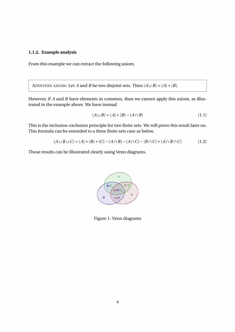
|A∪B ∪C | = |A|+ |B |+ |C |− |A∩B |− |A∩C |− |B ∩C |+ |A∩B ∩C | (1.2)
Those results can be illustrated clearly using Venn diagrams.
Figure 1: Venn diagrams
4
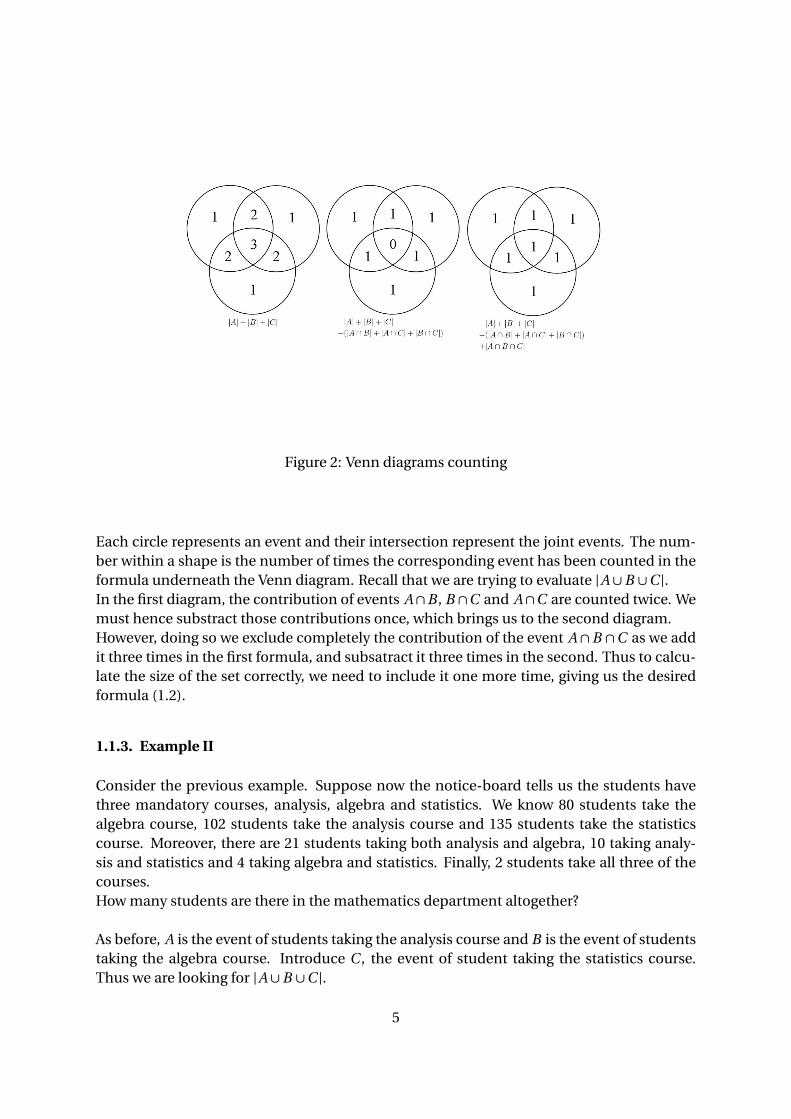
Figure 2: Venn diagrams counting
Each circle represents an event and their intersection represent the joint events. The num-ber within a shape is the number of times the corresponding event has been counted in theformula underneath the Venn diagram. Recall that we are trying to evaluate |A∪B ∪C |.In the first diagram, the contribution of events A∩B , B ∩C and A∩C are counted twice. Wemust hence substract those contributions once, which brings us to the second diagram.However, doing so we exclude completely the contribution of the event A∩B ∩C as we addit three times in the first formula, and subsatract it three times in the second. Thus to calcu-late the size of the set correctly, we need to include it one more time, giving us the desiredformula (1.2).
1.1.3. Example II
Consider the previous example. Suppose now the notice-board tells us the students havethree mandatory courses, analysis, algebra and statistics. We know 80 students take thealgebra course, 102 students take the analysis course and 135 students take the statisticscourse. Moreover, there are 21 students taking both analysis and algebra, 10 taking analy-sis and statistics and 4 taking algebra and statistics. Finally, 2 students take all three of thecourses.How many students are there in the mathematics department altogether?
As before, A is the event of students taking the analysis course and B is the event of studentstaking the algebra course. Introduce C , the event of student taking the statistics course.Thus we are looking for |A∪B ∪C |.
5
From the wording of our problem, we know the single event’s contribution |A| = 102, |B | =80, |C | = 135, and the joint event’s contribution |A∩B | = 21, |A∩B | = 10, |A∩B | = 4 and|A∩B ∩C | = 2.Applying the formula for three finite sets case,
|A∪B ∪C | = |A|+ |B |+ |C |− |A∩B |− |A∩C |− |B ∩C |+ |A∩B ∩C |= 102+80+135−21−10−4+2
= 284
(1.3)
Hence there are 284 students in the mathematics department.The example we carried out is one of the many applications of the inclusion-exclusion prin-ciple, raising awareness to the multiplicity of problems that can be solved by it. We will havea closer look at some applications after a more formal definition of the principle. Indeed,the two initial formulae can be generalised to the inclusion-exclusion principle for n finitesets.
1.2. The Inclusion-Exclusion Principle
THEOREM: Let A1, A2, ..., An be finite subsets of a universe A. Then∣∣∣∣∣ n⋃i=1
Ai
∣∣∣∣∣= n∑i=1
|Ai |−∑
1≤i< j≤n
∣∣Ai ∩ A j∣∣+ ∑
1≤i< j<k≤n
∣∣Ai ∩ A j ∩ Ak∣∣
− . . .+ (−1)n−1 |A1 ∩ . . .∩ An |(1.4)
Before proving this result, let us introduce another expression of the combinatorial inclusion-exclusion.
COROLLARY 1: Let A1, A2, ..., An be finite subsets of a universe A. Then∣∣∣∣∣ n⋂i=1
Ai
∣∣∣∣∣=|A|−n∑
i=1|Ai |+
∑1≤i< j≤n
∣∣Ai ∩ A j∣∣− ∑
1≤i< j<k≤n
∣∣Ai ∩ A j ∩ Ak∣∣
+ . . .+ (−1)n |A1 ∩ . . .∩ An |(1.5)
Where Ai is the complement of Ai
PROOF: Define B =⋃ni=1 Ai . Then by De Morgan’s Law,
B =n⋃
i=1Ai =
n⋂i=1
Ai (1.6)
6
From the addition axiom, since B ∩B =; and A = B ∪B we have
|A| = |B |+ |B ||B | = |A|− |B |∣∣∣∣∣ n⋂
i=1Ai
∣∣∣∣∣= |A|−∣∣∣∣∣ n⋃i=1
Ai
∣∣∣∣∣(1.7)
Hence the result
�
Similarly, we can derive a statistical formulation of the inclusion-exclusion principle as be-low.
COROLLARY 2: Let A1, A2, ..., An be finite events of a probability space A. Then
Pr
(n⋃
i=1Ai
)=
n∑i=1
Pr (Ai )−∑
1≤i< j≤nPr
(Ai ∩ A j
)+ ∑1≤i< j<k≤n
Pr(
Ai ∩ A j ∩ Ak)
− . . .+ (−1)n−1Pr (A1 ∩ . . .∩ An)
(1.8)
PROOF: By the frequency probability,
Pr (Ai ) = nAi
nA(1.9)
Where nA is the total number of trials, hence nA = |A|; and nAi is the number of trials wherethe event Ai occurs, hence nAi = |Ai |.Thus the desired result follows automatically dividing both sides of the inclusion-exclusionprinciple’s general formula by |A|.
�
All of the above formulations of the inclusion-exclusion principle are proven to be equiva-lent. We shall now prove the general result.
1.3. Proof of The Inclusion-Exclusion Principle
There are multiple ways to prove the inclusion-exclusion principle. We will examine threeof those. We will use a combinatorial approach for the first proof, for the second one we willuse indicator funtions and the last proof will be shown inductively.
1.3.1. PROOF 1 - Combinatorial Approach
Each point x ∈ ⋃ni=1 Ai contributes once in
∣∣⋃ni=1 Ai
∣∣. Similarly, each point y ∉ ⋃ni=1 Ai con-
tributes zero times in∣∣⋃n
i=1 Ai∣∣. Adding together all the contributions, we find the set size
7
∣∣⋃ni=1 Ai
∣∣. Hence, in order to prove the inclusion-exclusion principle, we need to show thatevery x contributes once to the right hand side of the inclusion-exclusion formula, and thatevery y doesn’t bring any contribution to the equation.
Assume⋃n
i=1 Ai 6= ;. If⋃n
i=1 Ai = ;, it will suffice to show that every element brings nocontribution to the right hand side of the inclusion-exclusion formula.
Take x ∈ ⋃ni=1 Ai . Suppose x belongs to exactly m of the sets {Ai }n
i=1, 1 ≤ m ≤ n. Let uscount its contribution to every intersection of events.Clearly, point will be counted m times in
∑ni=1 |Ai |, once for each set to which it belongs.
For the contribution of x in∑.
1≤i< j≤n
∣∣Ai ∩ A j∣∣, the point will be counted once for every cou-
ple of sets in which it lies. Thus we need to calculate the number of couple of sets we cancreate from those m sets. Hence, the point is counted
(m2
)times in
∑.1≤i< j≤n
∣∣Ai ∩ A j∣∣.
Similarly, we can get that the point is counted(m
3
)times in
∑.1≤i< j<k≤n
∣∣Ai ∩ A j ∩ Ak∣∣ and
so on, until we reach the term containing m intersections, where the point is counted onlyonce as
(mm
)= 1.The terms containing more than m intersections will inevitably intersect with a set thatdoesn’t contain x, thus the point won’t belong to the intersection and won’t bear any contri-bution.Hence the total contribution of the point x is(
m
1
)−
(m
2
)+
(m
3
)− . . .+ (−1)m−1
(m
m
)(1.10)
Now using the binomial expansion (a+b)m =∑mk=0
(mk
)am−k bk for a = 1 and b =−1, we have
(1−1)m =m∑
k=0
(m
k
)1m−k (−1)k
0 =(
m
0
)−
(m
1
)+
(m
2
)−
(m
3
)+ . . .+ (−1)m
(m
m
)(
m
0
)=
(m
1
)−
(m
2
)+
(m
3
)− . . .+ (−1)m−1
(m
m
)
1 =(
m
1
)−
(m
2
)+
(m
3
)− . . .+ (−1)m−1
(m
m
)(1.11)
We have demonstrated that every point belonging to⋃n
i=1 Ai contributes exactly once to theright hand side of the formula.
Moreover, any point y ∉⋃ni=1 Ai doesn’t belong to any of the sets {Ai }n
i=1, hence doesn’t bearany contribution to any of the terms of the right hand side.
Hence the only points contributing to the formula are the points belonging to⋃n
i=1 Ai , andthey all contribute only once.
�
8
1.3.2. PROOF 2 - Indicator functions
First, let us define what we mean by an indicator function.
DEFINITION:Let A be a set. An indicator function I is a map from a set X to {0,1} such that
I {A}(x) ={
1 i f x ∈ A0 i f x ∉ A
(1.12)
Let A = ⋃ni=1 Ai . To prove the inclusion-exclusion principle, we first need to verify that the
following identity holds
I {A} =n∑
k=1(−1)k−1
∑I⊂{1,...,n}, |I |=k
I {AI } (1.13)
where AI =⋂i∈I Ai .
For x ∉ A, the left hand side of (1.13) equals 0. Since A is the union of all sets Ai and x ∉ A,we must have x ∉ Ai ∀i = 1 → n i.e. I {AI } = 0 ∀I ⊂ {1, ...,n}. Hence the right hand side of(1.13) is therefore also zero. Thus the identity is ture for all x ∉ A.Now let us consider x ∈ A. Suppose x belongs to m sets of A1, ..., An , 1 ≤ m ≤ n. For simplic-ity of notation say these m sets containing x are A1, ..., Am .Our problem reduces to showing that
1 =m∑
k=1(−1)k−1
∑I⊂{1,...,m},|I |=k
1 (1.14)
Let us look at the right hand side first.∑
I⊂{1,...,m},|I |=k 1 represents the number of possiblesubsets of {1, ...,m} of size k, which is exactly
(mk
).
Rewriting the right hand side of (1.14) using this result, we get
RHS =m∑
k=1(−1)k−1
(m
k
)(1.15)
Moreover, notice that 1 = (m0
).
9
Now
0 = (1−1)m
=m∑
k=0(−1)k
(m
k
)
=(
m
0
)+
m∑k=1
(−1)k
(m
k
)
= 1−m∑
k=1(−1)k−1
(m
k
)
1 =m∑
k=1(−1)k−1
(m
k
)(1.16)
Hence (1.13) holds for both x ∈ A and x ∉ A.
We have that every x ∈⋃ni=1 Ai will contribute once to the left hand side of (1.13), and every
x ∈ ⋂i∈I Ai will contribute to the right hand side of (1.13) through I {AI }. We have therefore
proven the inclusion-exclusion principle.
�
1.3.3. PROOF 3 - Induction
Let P (n) be the inclusion-exclusion general formula:∣∣∣∣∣ n⋃i=1
Ai
∣∣∣∣∣= n∑i=1
|Ai |−∑
1≤i< j≤n
∣∣Ai ∩ A j∣∣+ ∑
1≤i< j<k≤n
∣∣Ai ∩ A j ∩ Ak∣∣
− . . .+ (−1)n−1 |A1 ∩ . . . An∩|(1.17)
At n = 1, ∣∣∣∣∣ 1⋃i=1
Ai
∣∣∣∣∣=|Ai |
=1∑
i=1|Ai |
(1.18)
Hence P (1) is true.Similarly, from Example 1.1.1 and 1.1.3, we know that P (2) and P (3) are true.
Suppose now P (r ) is true, that is∣∣∣∣∣ r⋃i=1
Ai
∣∣∣∣∣= r∑i=1
|Ai |−∑
1≤i< j≤r
∣∣Ai ∩ A j∣∣+ ∑
1≤i< j<k≤r
∣∣Ai ∩ A j ∩ Ak∣∣
− . . .+ (−1)r−1 |A1 ∩ . . .∩ Ar |(1.19)
10
Then for n = r +1, using P (2) we have
|A1 ∪ A2 ∪ . . .∪ Ar ∪ Ar+1| =∣∣∣∣∣(
r⋃i=1
Ai
)∪ Ar+1
∣∣∣∣∣=
∣∣∣∣∣ r⋃i=1
Ai
∣∣∣∣∣+|Ar+1|−∣∣∣∣∣(
r⋃i=1
Ai
)∩ Ar+1
∣∣∣∣∣(1.20)
Using the intersection distributivity, one can write∣∣∣∣∣(
r⋃i=1
Ai
)∩ Ar+1
∣∣∣∣∣=∣∣∣∣∣ r⋃i=1
(Ai ∩ Ar+1)
∣∣∣∣∣ (1.21)
Hence, applying the inductive hypothesis∣∣∣∣∣ r⋃i=1
(Ai ∩ Ar+1)
∣∣∣∣∣= r∑i=1
|Ai ∩ Ar+1|−∑
1≤i< j≤r
∣∣Ai ∩ A j ∩ Ar+1∣∣
+ . . .+ (−1)r−1 |A1 ∩ . . .∩ Ar ∩ Ar+1|(1.22)
Putting the equations together, we get∣∣∣∣∣r+1⋃i=1
Ai
∣∣∣∣∣= r∑i=1
|Ai |−∑
1≤i< j≤r
∣∣Ai ∩ A j∣∣+ ∑
1≤i< j<k≤r
∣∣Ai ∩ A j ∩ Ak∣∣
− . . .+ (−1)r−1 |A1 ∩ . . .∩ Ar |
+ |Ar+1|−r∑
i=1|Ai ∩ Ar+1|+
∑1≤i< j≤r
∣∣Ai ∩ A j ∩ Ar+1∣∣
− . . .+ (−1)r |A1 ∩ . . .∩ Ar ∩ Ar+1|
(1.23)
Cleary, it follows that∣∣∣∣∣r+1⋃i=1
Ai
∣∣∣∣∣= r+1∑i=1
|Ai |−∑
1≤i< j≤r+1
∣∣Ai ∩ A j∣∣+ ∑
1≤i< j<k≤r+1
∣∣Ai ∩ A j ∩ Ak∣∣
− . . .+ (−1)r |A1 ∩ . . .∩ Ar +1|(1.24)
P (n) is true for n = 1,2 and is inductive. Hence P (n) is true for all n ∈N∗.
�
The large number of ways to prove this result makes us undertand how fundamental it is.Most of the combinatorics problems we encounter use the inclusion-exclusion principle.Let us examine a simple example.
1.4. Statistical example
Suppose Joe is a five years old child that every morning enjoys eating his Colopops cereals.One day, the Colopops brand decides to extend its marketing goals, and issues a card, at
11
random, of the very famous cartoon Polemon with every box of cereal. The total collectionof cards to become a master-collecter is n.As soon as Joe hears about the collecting cards, he urges his mother to buy him N boxes ofcereal, hoping to collect all the cards.What is the probability that Joe becomes a master-collector?
The total number of ways to allocate a Polemon card in each box of Colopops without anyconstraint is S = nN . Define now Ai to be the event that the i th card of the total Polemoncollection is not in any of the N boxes of Colopops.The event we are looking for is
⋂ni=1 Ai Then |Ai | = (n −1)N , as there are only n−1 choices of
cards for each box. Similarly, we have |Ai ∩ A j | = (n −2)N for i 6= j , with(n
2
)ways of creating
such couples; and for k intersections the size of the event is (n −k)N with(n
k
)distinct inter-
section.
Using the second formula of the inclusion-exclusion principle,∣∣∣∣∣ n⋂i=1
Ai
∣∣∣∣∣=S −n∑
i=1|Ai |+
∑1≤i< j≤n
∣∣Ai ∩ A j∣∣− ∑
1≤i< j<k≤n
∣∣Ai ∩ A j ∩ Ak∣∣
+ . . .+ (−1)n |A1 ∩ . . .∩ An |
=nN −(
n
1
)× (n −1)N +
(n
2
)× (n −2)N − . . .+ (−1)n × (n −n)N
=n∑
k=0(−1)k ×
(n
k
)× (n −k)N
(1.25)
Hence the probability of Joe becoming a master-collector is
Pr := Pr
(n⋂
i=1Ai
)=
∣∣∣⋂ni=1 Ai
∣∣∣S
=∑n
k=0(−1)k × (nk
)× (n −k)N
nN
(1.26)
What does this probability mean? Suppose the total collection is made of n = 7 cards, andJoe persuasively managed for his mother to buy N = 20 boxes of Colopops. Then Joe has aprobability of Pr = 0.7039 to become a master-collector.
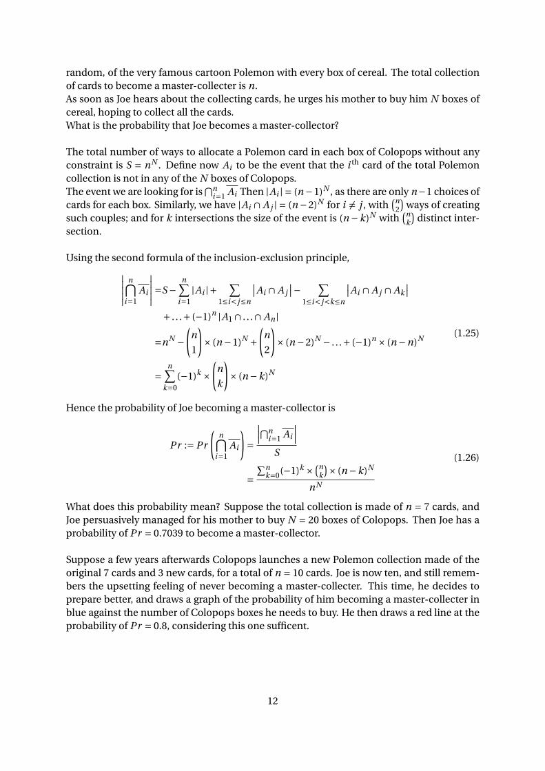
Suppose a few years afterwards Colopops launches a new Polemon collection made of theoriginal 7 cards and 3 new cards, for a total of n = 10 cards. Joe is now ten, and still remem-bers the upsetting feeling of never becoming a master-collecter. This time, he decides toprepare better, and draws a graph of the probability of him becoming a master-collecter inblue against the number of Colopops boxes he needs to buy. He then draws a red line at theprobability of Pr = 0.8, considering this one sufficent.
12
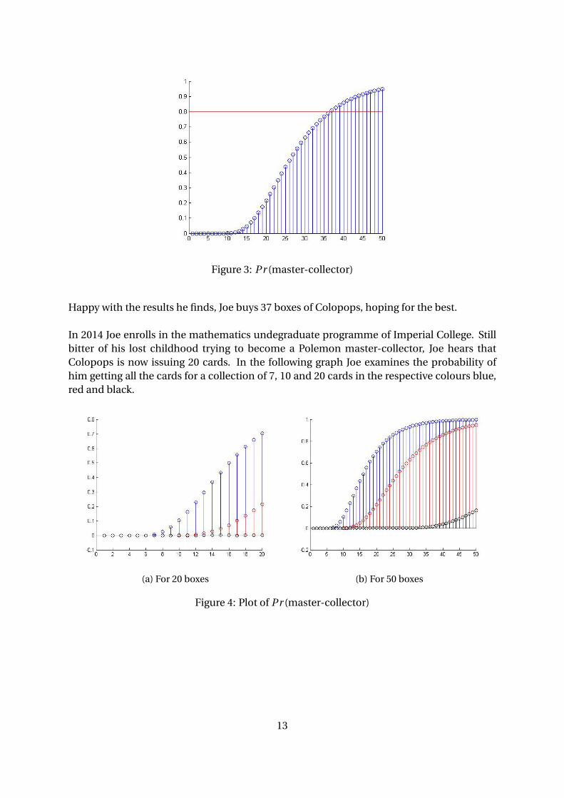
Figure 3: Pr (master-collector)
Happy with the results he finds, Joe buys 37 boxes of Colopops, hoping for the best.
In 2014 Joe enrolls in the mathematics undegraduate programme of Imperial College. Stillbitter of his lost childhood trying to become a Polemon master-collector, Joe hears thatColopops is now issuing 20 cards. In the following graph Joe examines the probability ofhim getting all the cards for a collection of 7, 10 and 20 cards in the respective colours blue,red and black.
(a) For 20 boxes (b) For 50 boxes
Figure 4: Plot of Pr (master-collector)
13
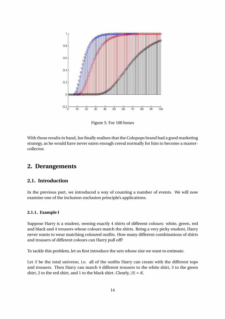
Figure 5: For 100 boxes
With those results in hand, Joe finally realises that the Colopops brand had a good marketingstrategy, as he would have never eaten enough cereal normally for him to become a master-collector.
2. Derangements
2.1. Introduction
In the previous part, we introduced a way of counting a number of events. We will nowexamine one of the inclusion-exclusion principle’s applications.
2.1.1. Example I
Suppose Harry is a student, owning exactly 4 shirts of different colours: white, green, redand black and 4 trousers whose colours match the shirts. Being a very picky student, Harrynever wants to wear matching coloured outfits. How many different combinations of shirtsand trousers of different colours can Harry pull off?
To tackle this problem, let us first introduce the sets whose size we want to estimate.
Let S be the total universe, i.e. all of the outfits Harry can create with the different topsand trousers. Then Harry can match 4 different trousers to the white shirt, 3 to the greenshirt, 2 to the red shirt, and 1 to the black shirt. Clearly, |S| = 4!.
14
Now set Aw the event where Harry matches the white shirt with the white trousers. ThenHarry can match 3 different trousers to the green shirt, 2 to the red shirt, and 1 to the blackshirt. Hence, |Aw | = 3!.
Similarly, set Ag , Ar , Ab to be the events where Harry matches respectively the greenshirt to the green trousers, the red shirt with the red trousers and the black shirt with theblack trousers. Then
|Aw | = |Ag | = |Ar | = |Ab | = 3! (2.1)
Now define the intersecting events of the form Ai ∩ A j . As two of the outfits are fixed, wehave 2 choices left for the third one, and one for the last one. I.e.
|Aw ∩ Ag | = |Aw ∩ Ar | = |Aw ∩ Ab | = |Ag ∩ Ar | = |Ag ∩ Ab | = |Ar ∩ Ab | = 2! (2.2)
Finally, fixing three of the outifts, we only have one choice for the fourth.
|Aw ∩ Ag ∩ Ar | = |Aw ∩ Ag ∩ Ab | = |Aw ∩ Ar ∩ Ab | = |Ag ∩ Ag ∩ Ab | = 1 (2.3)
And trivially
|Aw ∩ Ag ∩ Ar ∩ Ab | = 1 (2.4)
Coming back to our initial problematic, recall that we wish to find all the un-matching out-fits Harry can create. Hence we are looking for |Aw ∩ Ag ∩ Ar ∩ Ab |.
From our inclusion-exclusion formula, this is equal to
|S|−∑i|Ai |+
∑i
∑j|Ai ∩ A j |−
∑i
∑j
∑k|Ai ∩ A j ∩ Ak |+ |Aw ∩ Ag ∩ Ar ∩ Ab | (2.5)
for i = w, g ,r,b; j = w, g ,r,b j 6= i ; k = w, g ,r,b k 6= j k 6= i . Counting all differentcases as above and substituting by the respective st sizes
|Aw ∩ Ag ∩ Ar ∩ Ab | = 4!−4×3!+6×2!−4×1+1
= 9(2.6)
We have in this manner found the number of ways you can permute four elements, suchthat none of them is permuted to itself i.e. no shirt matches the trousers. This is called aderangement of four elements.
2.1.2. Example II
Let us now try to generalise the formula found above for n elements. Suppose Harry owns noutfits. How many different combinations of un-matching shirts and trousers can he wearsuch that no shirt matches the trousers?
The total universe S is now |S| = n!.
15
Define Ai to be the event that Harry is wearing the shirt i with the trousers i . The valuewe are looking for is:
∣∣∣A1 ∩ A2 ∩ ...∩ An
∣∣∣= |S|−n∑
i=1|Ai |+
n∑i=1
∑j<i
|Ai ∩ A j |− . . .+ (−1)n
∣∣∣∣∣ n⋂i+1
Ai
∣∣∣∣∣ (2.7)
Considering |Ai |, Harry has one choice of trousers for the shirt i , n−1 choices for any secondshirt, n −2 for any third shirt and so on. Hence,
|Ai | = 1× (n −1)× (n −2)× ...×2×1
= (n −1)!(2.8)
Similarly, consider |Ai∩A j |. Then for the shirts i and j Harry has only one choice of trousers;for any third shirt he has n −2 choices and so on. Clearly,
|Ai ∩ A j | = (n −2)! (2.9)
|Ai ∩ A j ∩ Ak | = (n −3)! (2.10)
... (2.11)
Now the inclusion-exclusion formula requires us to know the sum of all the different in-tersections. Hence we need to count the number of different ways we can write
⋂Ak for i
elements. This is no other than(n
i
).
The number of different combinations of un-matching outfits Harry can wear is∣∣∣∣∣ n⋂k=1
Ai
∣∣∣∣∣= N −n∑
k=1|Ak | +
n∑k=1
k−1∑j|Ak ∩ A j |− . . .+ (−1)n
n⋂k=1
|Ak |
= n! −(
n
1
)(n −1)! +
(n
2
)(n −2)! − . . .+ (−1)n
(n
n
)(n −n)!
=n∑
k=0(−1)k
(n
k
)(n −k)!
=n∑
k=0(−1)k n!
(n −k)! k !(n −k)!
= n!n∑
k=0
(−1)k
k !
(2.12)
This number is the number of derangements of the outfits of Harry.
2.2. Derangements
16
DEFINITION: A derangement is a permutation that doesn’t allow any fixed point.
THEOREM: The number of derangements of a set {1, . . . ,n} is given by the formula
D(n) = n!n∑
k=0
(−1)k
k !(2.13)
This result has been proven thorugh the example above.
2.3. Important results
2.3.1. Statistical results
One of the most straightforward applications of this results is statistical.Consider all the permutations of the set N := {1, . . . ,n}. What is the probability that the cho-sen permutation is a derangement?
Call A the event of a derangement. We know that out of n! permutations, D(n) are derange-ments. Hence
Pr (A) = D(n)
n!
= n!∑n
k=0(−1)k
k !
n!
=n∑
k=0
(−1)k
k !
(2.14)
Now considering the limit as n goes to infinity,
limn→∞
n∑k=0
(−1)k
k != exp(−1) = e−1 (2.15)
Furthermore, the series is known to converge very fast. We know that
e−1 = 0.36787944117...
Estimating∑n
k=0(−1)k
k ! for n = 8, we get
8∑k=0
(−1)k
k != 0.3679 (2.16)
The value we get is already accurate enough for most applications.In the following figures, Plot 1 is the plot of the value of e−1 and the values of Pr (A) from 0to 10 and Plot 2 is the plot of the absolute difference
∣∣e−1 −Pr (A)∣∣ for Pr (A) from 0 to 10.
17

(a) Plot 1 (b) Plot 2
Figure 6: Derangement probability analysis
We can conclude that for n big enough, choosing a random permutation, the probability ofgetting a derangement is independent from the size of the set permuted.
For example, assume a blind secretary needs to put n letters into n envelopes. Then fromour analysis, the probability that he doesn’t put a single letter into the right envelope isPr (An) ≈ e−1 ≈ 0.37 for n large enough. This means he has approximately a chance outof six to get every single envelope wrong. One the other hand, the chances of him putting allthe letters into the right envelope is Pr (Bn) = 1/n!. Hence, from the moment the secretaryhas more than four letter to send, he has more chances to mis-send all of them than gettingall of them right as Pr (B4) = 1/4! = 0.417. We would then recommend to avoid assigning thetask of sending off the mail to blind secretaries.
2.3.2. Recurrence relations
In the last part we saw how the general formula could easily be approximated with the expo-nential function. The result is useful when we have a calculator, but can we derive a formulathat we can calculate by hand?
18
From the combinatorics nature of our formula,
D(n) = n!n∑
k=0
(−1)k
k !
= n
[(n −1)!
n∑k=0
(−1)k
k !
]
= n
[(n −1)!
n−1∑k=0
(−1)k
k !+ (n −1)!
(−1)n
n!
]
= n
[D(n −1)+ (−1)n
n
]= nD(n −1)+ (−1)n
(2.17)
This result allows us to calculate simply the first values of the number of derangements of aset.For n = 1, one can rearrange one element in one single way, which is going to be the identity.Hence D(1) = 0. It follows that
D(2) = 2D(1)+ (−1)2
= 2×0+1 = 1(2.18)
D(3) = 3D(2)+ (−1)3
= 3−1 = 2(2.19)
D(4) = 4D(3)+ (−1)4
= 4×2+1 = 9(2.20)
D(5) = 5D(4)+ (−1)5
= 5×9−1 = 44(2.21)
D(6) = 6D(5)+ (−1)6
= 6×44+1 = 265(2.22)
D(7) = 7D(6)+ (−1)7
= 7×265−1 = 1854(2.23)
D(8) = 8D(7)+ (−1)8
= 8×1854+1 = 14833
...
(2.24)
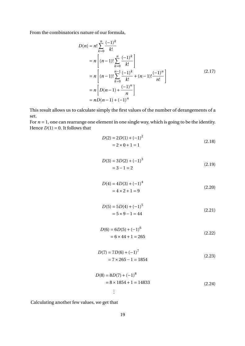
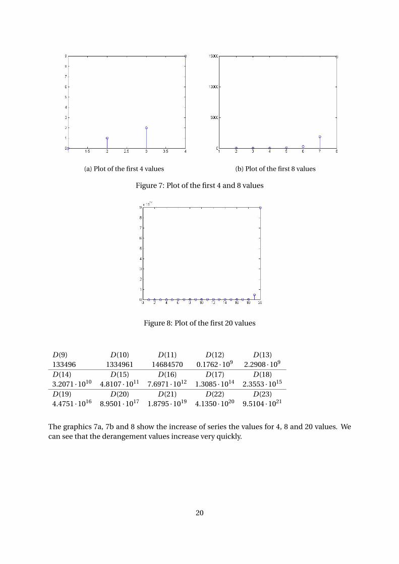
Calculating another few values, we get that
19
(a) Plot of the first 4 values (b) Plot of the first 8 values
Figure 7: Plot of the first 4 and 8 values
Figure 8: Plot of the first 20 values
D(9) D(10) D(11) D(12) D(13)133496 1334961 14684570 0.1762 ·109 2.2908 ·109
D(14) D(15) D(16) D(17) D(18)3.2071 ·1010 4.8107 ·1011 7.6971 ·1012 1.3085 ·1014 2.3553 ·1015
D(19) D(20) D(21) D(22) D(23)4.4751 ·1016 8.9501 ·1017 1.8795 ·1019 4.1350 ·1020 9.5104 ·1021
The graphics 7a, 7b and 8 show the increase of series the values for 4, 8 and 20 values. Wecan see that the derangement values increase very quickly.
20
2.4. Further work
Let us now consider one last example. Consider a class of 10 students. The professor decidesto test the students, and make them mark their own papers. In order to avoid cheating, theprofessor would like to avoid giving any student its own paper.
How many ways does the professor have to redistribute the papers?This is a simple derangement problem. From the above calculations, the professor hasD(10) = 133,496 ways to redistribute the papers.
However, the school the professor teaches in is a very small school, and each pair of stu-dents share a table. In order to avoid any kind of cheating, the professor doesn’t want eachstudent nor its neighbour to have the student’s paper.
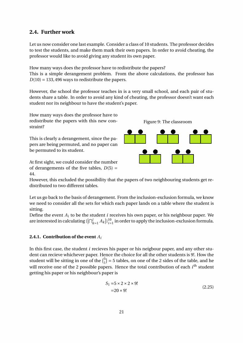
Figure 9: The classroom
How many ways does the professor have toredistribute the papers with this new con-straint?
This is clearly a derangement, since the pa-pers are being permuted, and no paper canbe permuted to its student.
At first sight, we could consider the numberof derangements of the five tables, D(5) =44.However, this excluded the possibility that the papers of two neighbouring students get re-distributed to two different tables.
Let us go back to the basis of derangement. From the inclusion-exclusion formula, we knowwe need to consider all the sets for which each paper lands on a table where the student issitting.Define the event Ai to be the student i receives his own paper, or his neighbour paper. Weare interested in calculating {
∣∣⋂ik=1 Ak
∣∣}10i=1 in order to apply the inclusion-exclusion formula.
2.4.1. Contribution of the event Ai
In this first case, the student i recieves his paper or his neigbour paper, and any other stu-dent can recieve whichever paper. Hence the choice for all the other students is 9!. How thestudent will be sitting in one of the
(51
) = 5 tables, on one of the 2 sides of the table, and hewill receive one of the 2 possible papers. Hence the total contribution of each i th studentgetting his paper or his neighbour’s paper is
S1 =5×2×2×9!
=20×9!(2.25)
21
2.4.2. Contribution of the event Ai ∩ A j
This case represent the situation where students i and j receive their own work, or theirneighbour’s work. We will then have 8! ways to distribute the other papers. We can distin-guish two cases, either the two students are sitting at the same table, or they are sitting inseparate tables.In the first case, the i th student will be sitting at one of the
(51
)= 5 tables, on one of the 2 sidesof the table. The j th student will only have one choice of positioning since he needs to be thei th student’s neighbour. Now student i can either receive his own work, or his neighbour’swork. However, we are counting each combination twice. So we need to multiply and divideby two, i.e. multiply by one.In the second case, the i th and j th student will have a choice of
(52
) = 10 tables, and each ofthem will be on one of the 2 sides of their respective table. Finally, each one will receive oneof the 2 possible papers.Hence, the contribution is
S2 =(5×2+10×22 ×22)×8!
=170×8!(2.26)
2.4.3. Contribution of the event Ai ∩ A j ∩ Ak
Consider now the case where some students i , j and k receive their own or their neighbour’swork. Then there are 7! ways to distribute the remaining papers. There are two distinguish-able cases, either two of the students are sitting at the same table, or they are all sitting apart.In the first case, the two first students will be sitting at one of the
(51
)= 5 tables and the third
student will be sitting at one of the(4
1
) = 4 remaining tables, on one of the 2 sides of the ta-ble. Each student will be given one of the 2 relevant papers. In the case of the neighbouringstudents, this will ony give us two choices instead of four, as once we choose which paperto give to one of the students, we only have 1 choice of paper for the second student. Noticethat this time, we are avoiding counting the fact that the two neighbouring students could bepicked in the opposite way. This is because it bears no importance which student is pickedfirst. If we pick a table and pick two students sitting at the table, then we will only have onechoice for the two students to pick. We will assume this reasoning for the following cases.In the second case, the three students will have
(53
) = 10 choices of tables distribution, eachof them will be on one of the 2 sides of the table and they will all receive one of the 2 papersconsidered.Hence the contribution is
S3 =(5×4×2×22 +10×23 ×23)×7!
=800×7!(2.27)
2.4.4. Contribution of the event Ai ∩ A j ∩ Ak ∩ Al
For this event, there are 6! ways to distribute the 6 remaining papers. The 3 distinguishablecases are all four students sit at different tables, two students are stitting at the same table
22
and two other are sitting at different tables and all students are sitting two by two at the sametwo tables.In the first case, the students will be sitting at one of the
(54
) = 5 possible table disposition,one of the 2 sides of the table, and they will be given one of the 2 relevant papers.In the second case, the students will be sitting at one of the
(51
)× (42
) = 5×6 = 30 table dis-position. For the students sitting apart, the professor will have a choice of 2 students. Eachstudent will be given one of the 2 relevant papers, and the choice of paper for the neighbour-ing students will depend on each other as in the previous event.In the third case, the students will be sitting at one of the
(52
) = 10 possible tables, and theywill be given one of the 2 relevant papers, depending on their neighbour’s choice as above.Hence the total contribution is
S4 =(5×24 ×24 +30×22 ×23 +10×22)×6!
=2280×6!(2.28)
2.4.5. Contribution of the event Ai ∩ A j ∩ Ak ∩ Al ∩ Am
As previously done, there are 5! ways to distribute the remaining 5 papers. The different waysto pick the students that will receive their own or their neighbour’s paper are as following.Either each student will be sitting on a different table, either two of them will be sitting ata same table, and three of them on separate tables, or four of them will be paired on tablesand one will be sitting separately.In the first case, we have a choice of
(55
)= 1 different ways to pick the five tables. Each studentwill be sitting on one of the 2 sides of the table, and will receive one of the 2 desired papers.In the second case, we have a choice of
(51
)×(43
)= 5×4 = 20 ways to pick the tables. The threeindependent students will be sitting on one of the 2 sides of the table, and each will receiveone of the 2 papers, bearing in mind the dependence of the neighbouring student’s choice.In the third case, we have a choice of
(52
)× (31
) = 10×3 = 30 ways of picking the tables. Theindependent student will be sitting on one of the 2 sides of the table, and each will receiveone of the 2 papers as above.Hence the total contribution is
S5 =(1×25 ×25 +20×23 ×24 +10×2×23)×5!
=2280×5!(2.29)
2.4.6. Other contributions
Similarly, one can calculate the remaining contributions with the following formula
Sn/(10−n)! = ∑ways to pick students
[ways to pick the tables
]×[
ways to select the independent students for each table]
×[ways to hand the relevant papers
](2.30)
23

We then have
S6
4!=
(5
1
)×
(4
4
)×24 ×25 [
2 neighbouring students + 4 independent students]
+(
5
2
)×
(3
2
)×22 ×24 [
4 neighbouring students + 2 independent students]
+(
5
3
)×
(2
0
)×20 ×23 [
6 neighbouring students + 0 independent students]
(2.31)
S6 = 4560×4! (2.32)
S7
3!=
(5
2
)×
(3
3
)×23 ×25 [
4 neighbouring students + 3 independent students]
+(
5
3
)×
(2
1
)×21 ×24 [
6 neighbouring students + 1 independent student] (2.33)
S7 = 3200×3! (2.34)
S8
2!=
(5
3
)×
(2
2
)×22 ×25 [
6 neighbouring students + 2 independent students]
+(
5
4
)×
(2
0
)×20 ×24 [
8 neighbouring students] (2.35)
S8 = 1360×2! (2.36)
S9
1!=
(5
4
)×
(1
1
)×21 ×25 [
8 neighbouring students + 1 independent student]
(2.37)
S9 = 320×1! (2.38)
S10
0!=
(5
5
)×
(0
0
)×20 ×25 [
10 neighbouring students]
(2.39)
S10 = 32×0! (2.40)
Finally, the total number of possible ways of redistributing the papers is 10!.
24
2.4.7. Final result and analysis
From the inclusion-exclusion formula we have:
N =10!−S1 +S2 −S3 +S4 −S5 +S6 −S7 +S8 −S9 +S10
=10!−20×9!+170×8!−800×7!+2280×6!−4064×5!
+4560×4!−3200×3!+1360×2!−320×1!+32×0!
=440192
(2.41)
This method emphasises the limits of the formula we have previously derived. Indeed, assoon as we increase the number of constraints, we can no longer use the derangement for-mula. The latter only applies for simple derangements where the only constraint is the de-rangement itself. Other more complicated cases as the classroom problem that we havestudied require us to go back to the initial inclusion-exclusion formula and undergo tediouscalculations, increasing the risk of human errors.
However, in the next chapter we will present a new method using rook polynomials. Theadvantage of deriving another method is the possibility to create a simple algorithm in or-der to reduce the possibility of human error.
3. Rook Polynomials
3.1. Introduction
In order to better understand the mathematics behind rook polynomials, lets us first startwith a little everyday mathematicians problem.Assume Sofie, a mathematics undergraduate, is playing a game of English chess with herbest friend. Problematically, they know each other so well that you can predict each othersmoves with a 100% accurancy. Hence Sofie and her friend decide to modify the game inorder to make it more interesting. From now on they will allow the opponent to place theirrooks anywhere on the chessboard, ignoring the previous positioning. Furthermore, theywill be able to take out the opponents’ rooks as long as they are on the same row or column,regardless of the position of the other pieces.They quickly realise that it is quite tricky to position their rooks avoiding any vulnerable po-sitionings. In order to better understand her options, Sofie starts counting all the possibleways to arrange the rooks on the chessboard.Extending her approach, the student tries to imagine how to place 8 rooks on a full 8× 8chessboard such that the above criterion is fulfilled. After a little time, she comes the con-clusion that there are 8! ways to position such rooks without any rook attacking anotherrook. How did she reach this conclusion?
In this chapter, we will examine the number of ways to place different number of rooks onchessboards of different sizes and shapes, in order to formulate what we will define to berook polynomials.We will then use this information to estimate permutation and combina-torics problems.
25
3.2. Definition of Rook Polynomials
...
...
...
.
.
.
...
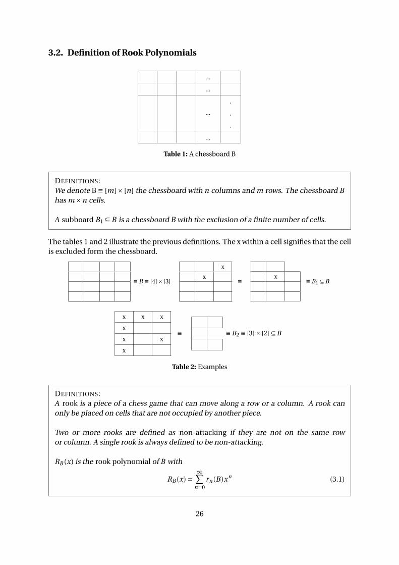
Table 1: A chessboard B
DEFINITIONS:We denote B ≡ [m]× [n] the chessboard with n columns and m rows. The chessboard Bhas m ×n cells.
A subboard B1 ⊆ B is a chessboard B with the exclusion of a finite number of cells.
The tables 1 and 2 illustrate the previous definitions. The x within a cell signifies that the cellis excluded form the chessboard.
≡ B ≡ [4]× [3]
x
x ≡ x ≡ B1 ⊆ B
x x x
x
x x
x
≡ ≡ B2 ≡ [3]× [2] ⊆ B
Table 2: Examples
DEFINITIONS:A rook is a piece of a chess game that can move along a row or a column. A rook canonly be placed on cells that are not occupied by another piece.
Two or more rooks are defined as non-attacking if they are not on the same rowor column. A single rook is always defined to be non-attacking.
RB (x) is the rook polynomial of B with
RB (x) =∞∑
n=0rn(B)xn (3.1)
26
where rk (B) is the number of ways k non-attacking identical rooks can be placed on achessboard B , and r0(B) = 1
LEMMA: Rk (B) = 0 ∀k > min(n,m) for any subboard Bi of B = [m]× [n]
PROOF: If we have more than min(n,m) rooks to place on the board, then at least two ofthem will be on a same row or column, and hence won’t be non-attacking.
3.2.1. Examples
Let us express the rook polynomial for the chessboards B1, B2 and B3.
Chessboard B1
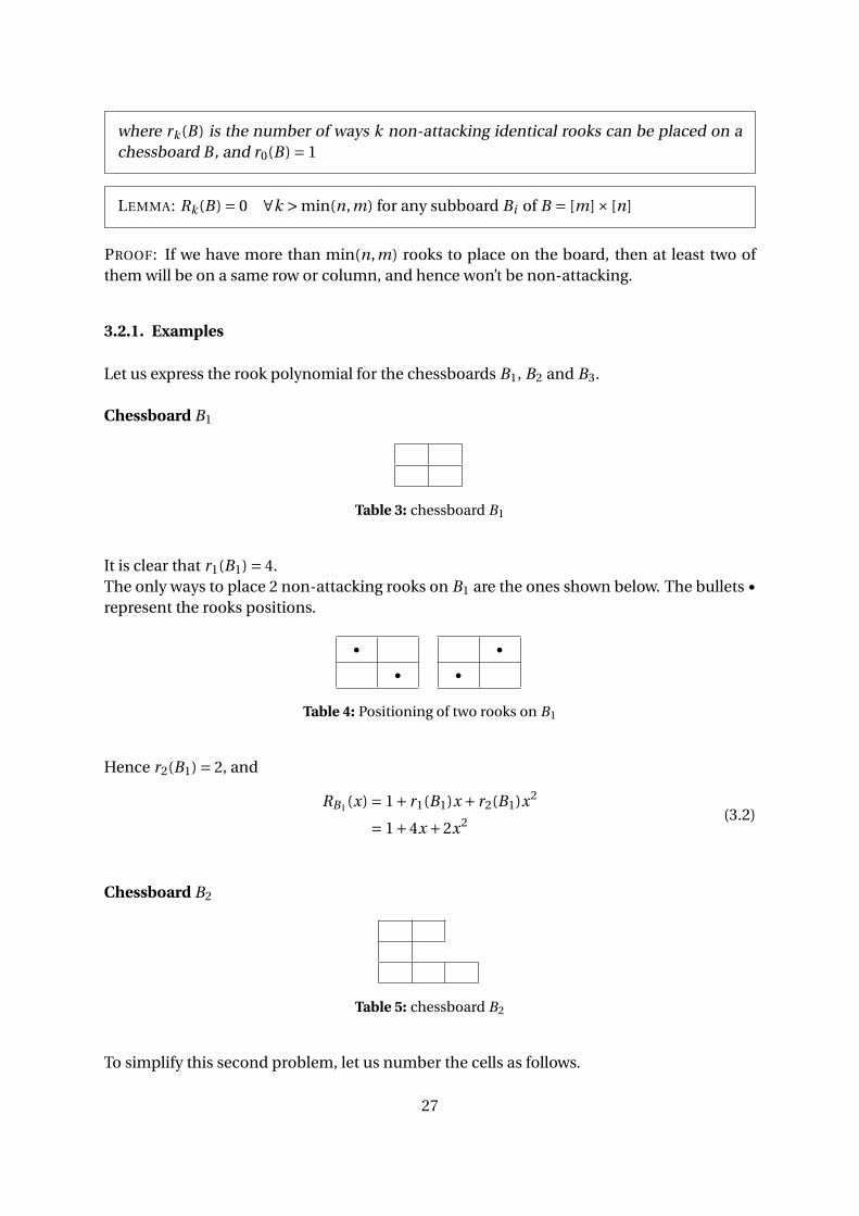
Table 3: chessboard B1
It is clear that r1(B1) = 4.The only ways to place 2 non-attacking rooks on B1 are the ones shown below. The bullets •represent the rooks positions.
••
••
Table 4: Positioning of two rooks on B1
Hence r2(B1) = 2, and
RB1 (x) = 1+ r1(B1)x + r2(B1)x2
= 1+4x +2x2 (3.2)
Chessboard B2
Table 5: chessboard B2
To simplify this second problem, let us number the cells as follows.
27
1 2
3
4 5 6
Table 6: Numbering of cells of B2
Denote S be the set of all possible non-attacking rooks placements for 2 rooks. Then
S = {(1,5), (1,6), (2,3), (2,4), (2,6), (3,5), (3,6)} (3.3)
We have |S| = 7, hence r2(B) = 7.Similarly, denote S′ the set of possible non-attacking rooks placement for 3 rooks
S′ = {(2,3,6)} (3.4)
There is a single possibility to position 3 rooks, hence r3(B) = 1.Thus
RB2 (x) = 1+ r1(B2)x + r2(B2)x2 + r3(B2)x3
= 1+6x +7x3 +x3 (3.5)
Chessboard B3
x x x ... x
x x x ... x
x x x ... x
x x x ... x
.
.
.
.
.
.
.
.
.
.
.
.
...
...
...
.
.
.
x x x x ...
...
...
...
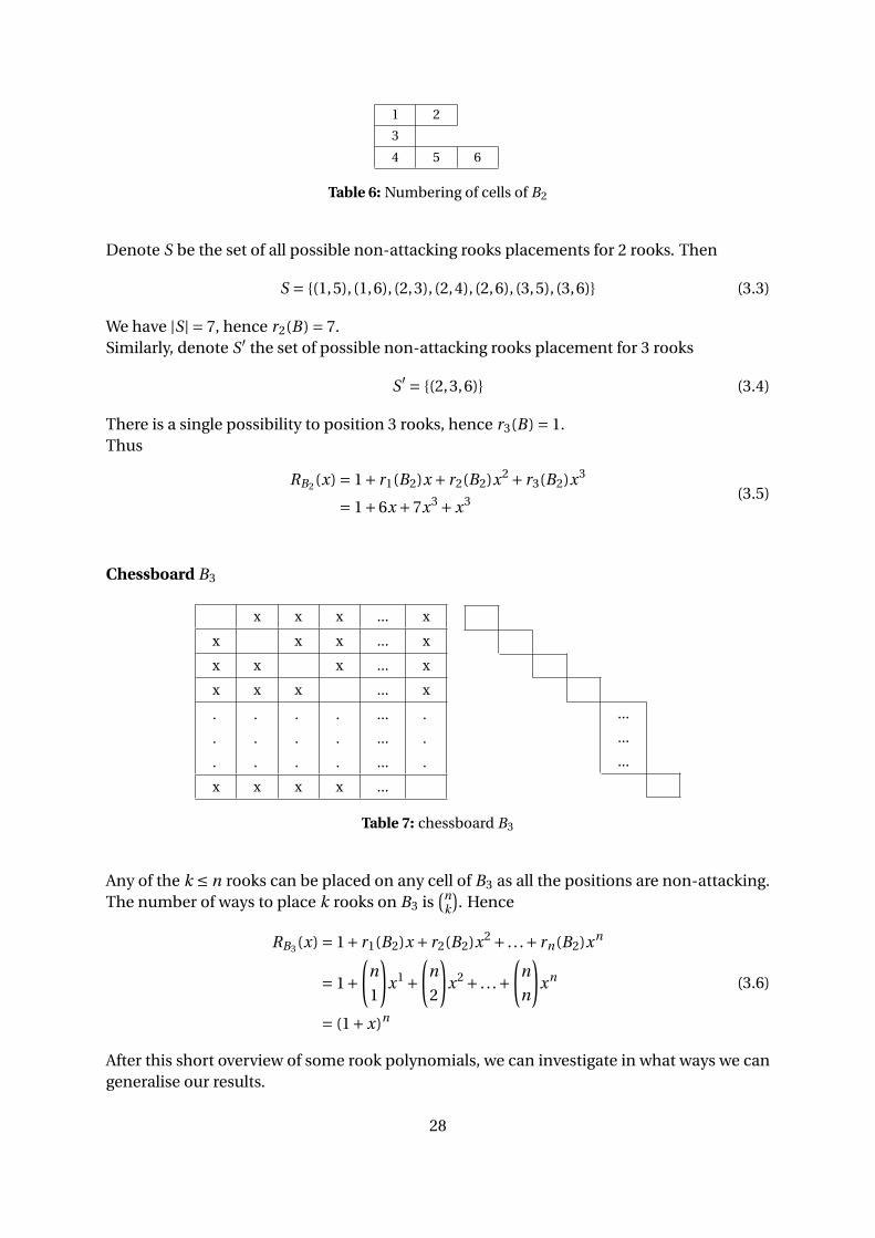
Table 7: chessboard B3
Any of the k ≤ n rooks can be placed on any cell of B3 as all the positions are non-attacking.The number of ways to place k rooks on B3 is
(nk
). Hence
RB3 (x) = 1+ r1(B2)x + r2(B2)x2 + . . .+ rn(B2)xn
= 1+(
n
1
)x1 +
(n
2
)x2 + . . .+
(n
n
)xn
= (1+x)n
(3.6)
After this short overview of some rook polynomials, we can investigate in what ways we cangeneralise our results.
28

3.2.2. Full Chessboards
DEFINITIONS:A chessboard B is a full chessboard if it is a rectangular chessboard without any ex-cluded cells.
A chessboard B = [m]× [n] is a squared chessboard if m = n
For example, the following is a full squared chessboard.
Table 8: Chessboard example
PROPERTY: Let B be a full chessboard. Then the following hold.1- The highest degree of the rook polynomial of a full chessboard is min(m,n).2- The value for any other coefficient is determined by rk (B) = (m
k
)(nk
)k ! with 0 ≤ k ≤
min(m,n).
PROOF:1- Without loss of generality, assume m ≥ n, hence min(m,n) = n. Call the highest degree ofthe rook polynomial h.
One of the ways we can allocate all the rooks on the chessboard is on the diagonal, suchthat they take the positions {(1,1), (2,2), . . . , (n,n)}. Hence h ≥ n.On the other hand, assume by contradiction that h > n. Say h = n +1. Place first n rooks,one for each column. You then have one rook left, but no column witout any rooks. Hencethe last rook will automatically be in an attacking position. Hence h < n +1. Thus h = n =min(m,n).
2- To place our k rooks, we have a choice of(m
k
)distinct rows, and
(nk
)rows. We then need
to decide on which cell we want to put the rook on the first column. As there are k possiblerows to choose from, we have k choices of cells. Moving on to the next column, we now havek −1 choices, and so on. Eventually we will have k(k −1)(k −2)...(2)(1) ways of placing theserooks on the chosen rows and columns in a non-attacking positioning. Hence
rk (B) =(
m
k
)(n
k
)k ! (3.7)
�
29
3.2.3. Some usefull theorems
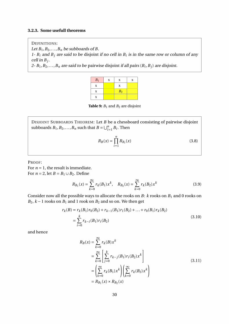
DEFINITIONS:Let B1,B2, . . . ,Bn be subboards of B .1- Bi and B j are said to be disjoint if no cell in Bi is in the same row or column of anycell in B j .2- B1,B2, . . . ,Bn are said to be pairwise disjoint if all pairs (Bi ,B j ) are disjoint.
B1 x x x
x x
x B2
x
Table 9: B1 and B2 are disjoint
DISJOINT SUBBOARDS THEOREM: Let B be a chessboard consisting of pairwise disjointsubboards B1,B2, . . . ,Bn such that B =⋃n
i=1 Bi . Then
RB (x) =n∏
i=1RBi (x) (3.8)
PROOF:For n = 1, the result is immediate.For n = 2, let B = B1 ∪B2. Define
RB1 (x) =∞∑
k=0rk (B1)xk , RB2 (x) =
∞∑k=0
rk (B2)xk (3.9)
Consider now all the possible ways to allocate the rooks on B : k rooks on B1 and 0 rooks onB2, k −1 rooks on B1 and 1 rook on B2 and so on. We then get
rk (B) = rk (B1)r0(B2)+ rk−1(B1)r1(B2)+ . . .+ r0(B1)rk (B2)
=k∑
i=0rk−i (B1)ri (B2)
(3.10)
and hence
RB (x) =∞∑
k=0rk (B)xk
=∞∑
k=0
[k∑
j=0rk− j (B1)ri (B2)xk
]
=( ∞∑
k=0rk (B1)xk
)( ∞∑k=0
rk (B2)xk
)= RB1 (x)×RB2 (x)
(3.11)
30
Finally, for any n > 2, assuming the formula for⋃n−1
i=1 Bi , let B = (⋃n−1i=1 Bi
)∪Bn . Then usingthe result we derived, we can show that
RB (x) = R⋃n−1i=1 Bi
(x)×RBn (x)
=n∏
i=1RBi (x)
(3.12)
We can conclude that since the result is true for n = 1,2 and is inductive, the result is true forany integer n.
�
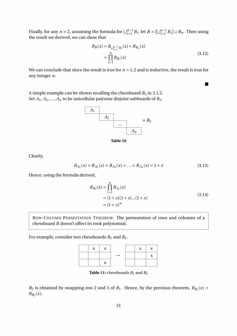
A simple example can be shown recalling the chessboard B3 in 3.1.2.Set A1, A2, . . . , An to be unicellular pairwise disjoint subboards of B3.
A1
A2
...
An
≡ B3
Table 10
Clearly,
RA1 (x) = RA2 (x) = RA3 (x) = . . . = RAn (x) = 1+x (3.13)
Hence, using the formula derived,
RB3 (x) =n∏
i=1RAi (x)
= (1+x)(1+x)...(1+x)
= (1+x)n
(3.14)
ROW-COLUMN PERMUTATION THEOREM: The permutation of rows and columns of achessboard B doesn’t affect its rook polynomial.
For example, consider two chessboards B1 and B2.
x x
x
→x x
x
Table 11: chessboards B1 and B2
B2 is obtained by swapping row 2 and 3 of B1. Hence, by the previous theorem, RB1 (x) =RB2 (x).
31
PROOF: Let B1 and B2 be two chessboards, such that we can obtain one by a single per-mutation of rows and columns of the other. Then the number of ways you can place eachnumber k of rooks doesn’t vary. Hence rkB1
= rkB2, implying that RB1 (x) = RB2 (x).
We can then operate another permutation on B2 to get B3 and so on. Applying the same rea-soning, all the rook polynomials will be equal. Hence any permutation of rows and columnsconserves the rook polynomial of the chessboard.
�
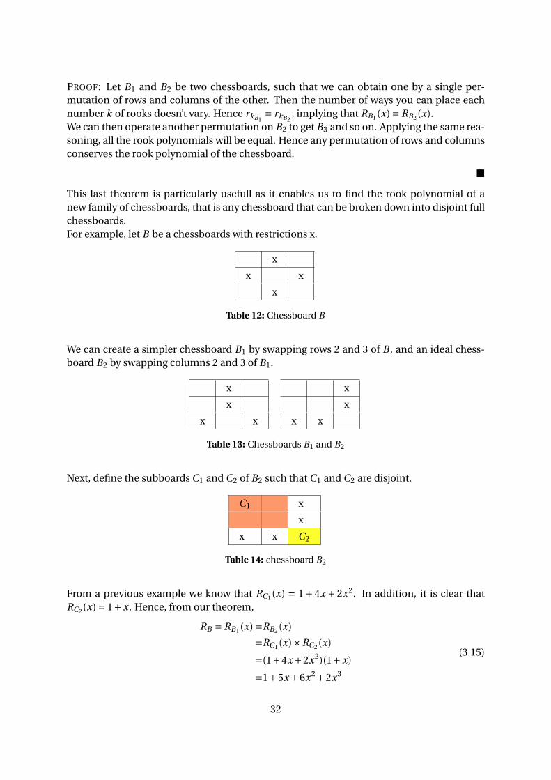
This last theorem is particularly usefull as it enables us to find the rook polynomial of anew family of chessboards, that is any chessboard that can be broken down into disjoint fullchessboards.For example, let B be a chessboards with restrictions x.
x
x x
x
Table 12: Chessboard B
We can create a simpler chessboard B1 by swapping rows 2 and 3 of B , and an ideal chess-board B2 by swapping columns 2 and 3 of B1.
x
x
x x
x
x
x x
Table 13: Chessboards B1 and B2
Next, define the subboards C1 and C2 of B2 such that C1 and C2 are disjoint.
C1 x
x
x x C2
Table 14: chessboard B2
From a previous example we know that RC1 (x) = 1+ 4x + 2x2. In addition, it is clear thatRC2 (x) = 1+x. Hence, from our theorem,
RB = RB1 (x) =RB2 (x)
=RC1 (x)×RC2 (x)
=(1+4x +2x2)(1+x)
=1+5x +6x2 +2x3
(3.15)
32
CELL DECOMPOSITION THEOREM: Let B be a chessboard, and a a cell of such board.Denote by B ′ the subboard of B that excludes the row and column containing a, and byB ′′ the subboard of B which excludes the cell a. Then the following holds.
RB (x) = xRB ′(x)+RB ′′(x) (3.16)
PROOF:RB ′(x) is equivalent to the rook polynomial of B given that there is a rook on a, and RB ′′(x) isequivalent to the rook polynomial of B given that there is not a rook on a.It follows that for k ≥ 1, rk−1(B ′) calculates the event that there are k − 1 rooks on B ′ and1 rook on a; and rk (B ′′) the event that there are k rooks on B ′′ and none on a. Hence thesum of those two terms is equal to the total number of ways to place k rooks on B , rk (B) =rk−1(B ′)+ rk (B ′′).Thus
RB (x) = r0(B ′′)+∞∑
k=1[rk−1(B ′)+ rk (B ′′)]xk
= xRB ′(x)+RB ′′(x)
(3.17)
�
Going back to the example above, set a to be the cell (2,2) on chessboard B . Notice that fromour definition, B ′ ≡ B ′′. Hence
RB ′(x) = RB ′′(x) = 1+4x +2x2 (3.18)
RB (x) = xRB ′(x)+RB ′′(x) = x +4x2 +2x3 +1+4x +2x2
= 1+5x +6x2 +2x3 (3.19)
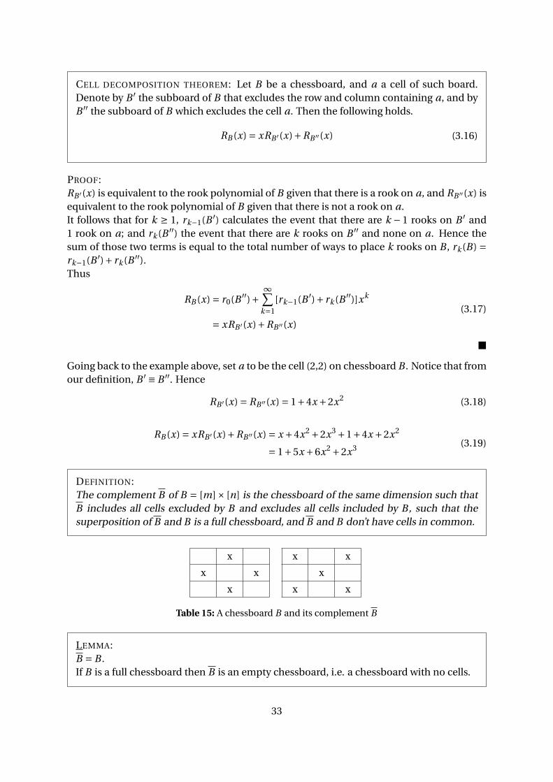
DEFINITION:The complement B of B = [m]× [n] is the chessboard of the same dimension such thatB includes all cells excluded by B and excludes all cells included by B , such that thesuperposition of B and B is a full chessboard, and B and B don’t have cells in common.
x
x x
x
x x
x
x x
Table 15: A chessboard B and its complement B
LEMMA:B = B .If B is a full chessboard then B is an empty chessboard, i.e. a chessboard with no cells.
33
The proof of this lemma is immediate.
COMPLEMENT THEOREM: Let B be the complement of B = [m]× [n]. Then
rk (B) =k∑
i=0(−1)i
(m − i
k − i
)(n − i
k − i
)(k − i )!ri (B) (3.20)
PROOF: The idea behind this proof is to calculate the total ways to allocate k non-attackingrooks onto the [m]×[n] full chessboard, then substract all the ways to put 1 up to k rooks onB . Using the inclusion-exclusion principle, we will then be able to derive rk (B).
Call Q the full [m] × [n] chessboard. From the full chessboards property, we know thatrk (Q) = (m
k
)(nk
)k !. Let us now assign a number to each of the rooks. There are k ! ways to
do so. Thus the number of ways to allocate k numbered rooks onto a full chessboard is(mk
)(nk
)(k !)2.
Denote Ci the set of all placements of the rooks where the i th rook is on the board B , Ci ∩C j
the set of all placements of the rooks where the i th and j th rook is on the board B and so on.We are then interested in the event
⋂ki=1 Ci .
Considering the number assignment of them, we know that there are(k
i
)i !ri (B) ways to put
i numbered non-attacking rooks onto B . We then exclude the rows and columns of the irooks we already placed onto B from the full chessboard. Rearranging the remaining cells bypermutations and using the row-column permutation theorem, we are left with k − i rooksto allocate onto an [m − i ]× [n − i ] full chessboard. Thus the number of ways to place theremaining rooks is (
m − i
k − i
)(n − i
k − i
)[(k − i )!]2 (3.21)
Hence
|Ci | =(
k
1
)1!
(m −1
k −1
)(n −1
k −1
)[(k −1)!]2
∣∣Ci ∩C j∣∣= (
k
2
)2!
(m − i
k −2
)(n − i
k −2
)[(k −2)!]2
...
(3.22)
34
Using the second inclusion-exclusion formula derived in the first part of this paper:∣∣∣∣∣ k⋂i=1
Ci
∣∣∣∣∣=|Q|−k∑
i=1|Ci |+
∑1≤i< j≤k
∣∣Ci ∩C j∣∣− ∑
1≤i< j<m≤k
∣∣Ci ∩C j ∩Cm∣∣
+ . . .+ (−1)k |C1 ∩ . . .∩Ck |
k ! rk (B) =(
k
0
)0!
(m
k
)(n
k
)(k !)2r0(B)−
(k
1
)1!
(m −1
k −1
)(n −1
k −1
)[(k −1)!]2 r1(B)
+ . . .+ (−1)k
(k
k
)k !
(m −k
0
)(n −k
0
)[0!]2 rk (B)
=k∑
i=0(−1)i
(k
i
)i !
(m − i
k − i
)(n − i
k − i
)[(k − i )!]2 ri (B)
=k∑
i=0(−1)i k !(k − i )!
(m − i
k − i
)(n − i
k − i
)ri (B)
rk (B) =k∑
i=0(−1)i (k − i )!
(m − i
k − i
)(n − i
k − i
)ri (B)
(3.23)
�
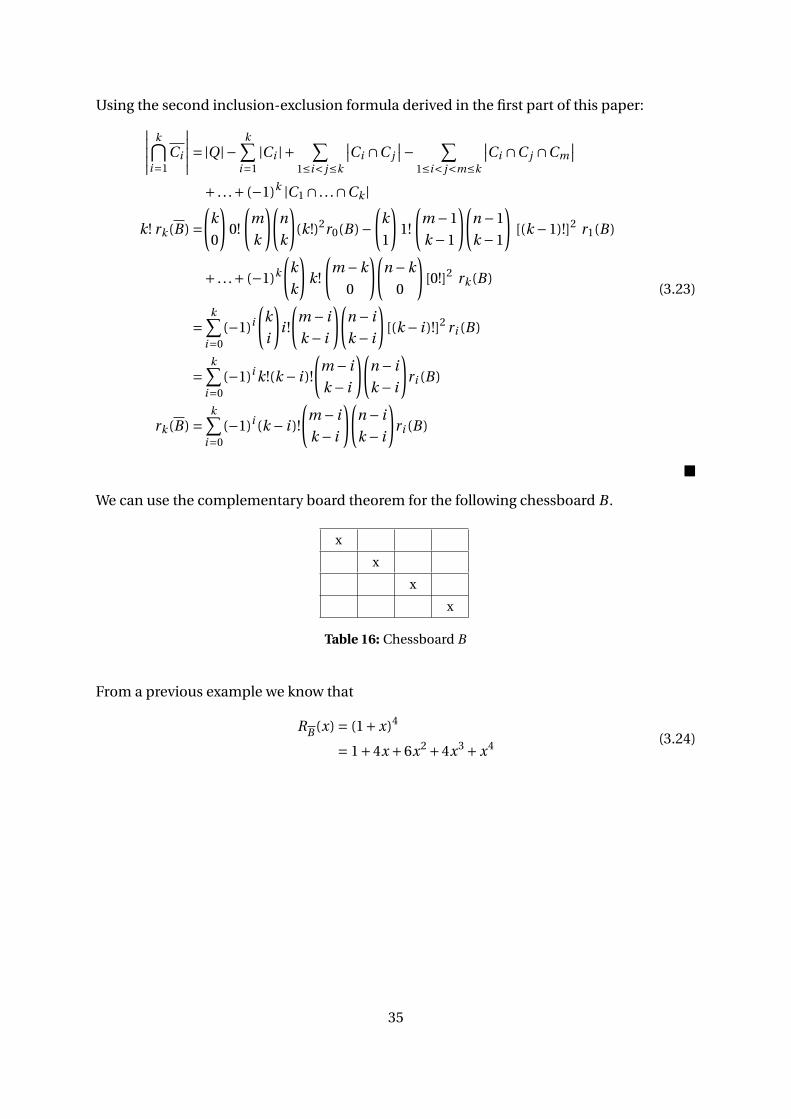
We can use the complementary board theorem for the following chessboard B .
x
x
x
x
Table 16: Chessboard B
From a previous example we know that
RB (x) = (1+x)4
= 1+4x +6x2 +4x3 +x4 (3.24)
35
Now
r2(B) =(
4
2
)(4
2
)2! r0(B)−
(3
1
)(3
1
)1! r1(B)+
(2
0
)(2
0
)0! r2(B)
= 72−36+6 = 42
r3(B) =(
4
3
)(4
3
)3! r0(B)−
(3
2
)(3
2
)2! r1(B)+
(2
1
)(2
1
)1! r2(B)−
(1
0
)(1
0
)0! r3(B)
= 96−72+24−4 = 44
r4(B) =(
4
4
)(4
4
)4! r0(B)−
(3
3
)(3
3
)3! r1(B)+
(2
2
)(2
2
)2! r2(B)−
(1
1
)(1
1
)1! r3(B)+
(0
0
)(0
0
)0! r4(B)
= 24−24+12−4+1 = 9(3.25)
Hence
RB (x) = 1+12x +42x2 +44x3 +9x4 (3.26)
THEOREM: Let B = [m]× [n] be a restricted chessboard admitting a non-empty comple-ment B . Then the number of ways to allocate k rooks onto B is
S(k) =k∑
i=0(−1)i (k − i )! ri (B) (3.27)
Let Q be the full [m]× [n] chessboard. Define Bi , the event of i numbered rooks being in therestricted chessboard B . Then by the inclusion-exclusion theorem,∣∣∣∣∣ k⋂
i=1Bi
∣∣∣∣∣=|Q|−k∑
i=1
∣∣∣Bi
∣∣∣+ ∑1≤i< j≤k
∣∣∣Bi ∩B j
∣∣∣− ∑1≤i< j<m≤k
∣∣∣Bi ∩B j ∩Bm
∣∣∣+ . . .+ (−1)k
∣∣∣B1 ∩ . . .∩Bk
∣∣∣=|Q|−S1 +S2 − . . .+ (−1)k Sk
(3.28)
Where Si is the sum of all the intersections of i elements.Note that Si is equal to the number of ways of choosing i restricted cells in distinct rowsand columns times the number of allocations of the rooks on the restricted board times thenumber of allocation of the remainding rooks on the full chessboard.
Si =(
k
i
)ri
(B
)(k − i )! (3.29)
Hence
S(k) :=∣∣∣∣∣ k⋂i=1
Bi
∣∣∣∣∣= k∑i=0
(−1)i (k − i )! ri (B) (3.30)
�
36
3.3. Examples and applications
Going back to the initial example used in part 2.4, we can show the correlation between rookpolynomials and derangements.Consider this time a class of k students. The professor of the class is looking for a way toredistribute the k papers to its students, whitout any of them getting their own back. Canwe translate this probem into a chessboard?
Let each column of the chessboard represent a student, and each row represent its paper.Hence if column i represent the student i , then the row i will represent the paper of the stu-dent i .
Now each cell is the allocation of paper the professor has in mind. Quite clearly, if the profes-sor gives paper i to the student j , then he won’t be able to give the same paper to any otherstudent. Vice-versa, if the student j receives the paper i , he won’t receive any other paper.This translates into allocating non-attacking rooks on the chessboard we have created.
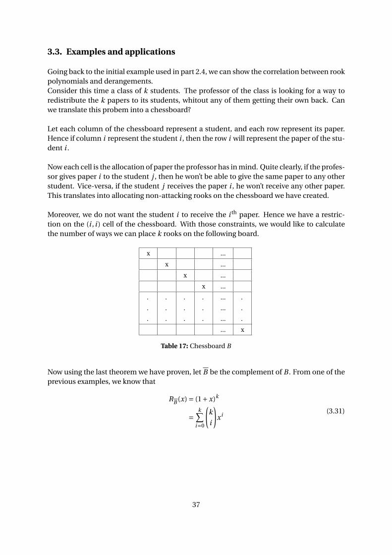
Moreover, we do not want the student i to receive the i th paper. Hence we have a restric-tion on the (i , i ) cell of the chessboard. With those constraints, we would like to calculatethe number of ways we can place k rooks on the following board.
x ...
x ...
x ...
x ...
.
.
.
.
.
.
.
.
.
.
.
.
...
...
...
.
.
.
... x
Table 17: Chessboard B
Now using the last theorem we have proven, let B be the complement of B . From one of theprevious examples, we know that
RB (x) = (1+x)k
=k∑
i=0
(k
i
)xi
(3.31)
37
Hence
D(k) := S(k) =k∑
i=0(−1)i (k − i )! ri (B)
=k∑
i=0(−1)i (k − i )!
(k
i
)
= k !k∑
i=0
(−1)i
i !
(3.32)
We have in this manner proven in a new way the derangement formula derived in a previ-ous part of this paper. Furthermore, rook polynomials can help us even further to evaluatederangments, as the limitations encountered by the additional constraint in part 2.3 are notas problematic for our chessboards.
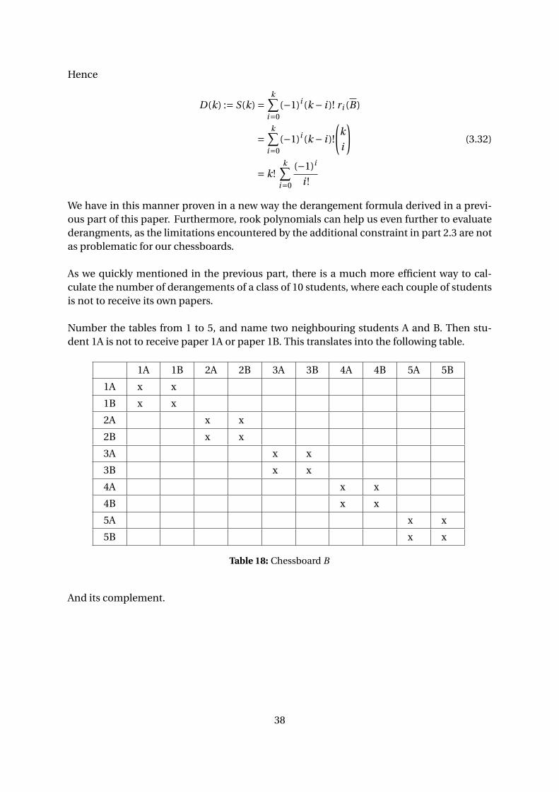
As we quickly mentioned in the previous part, there is a much more efficient way to cal-culate the number of derangements of a class of 10 students, where each couple of studentsis not to receive its own papers.
Number the tables from 1 to 5, and name two neighbouring students A and B. Then stu-dent 1A is not to receive paper 1A or paper 1B. This translates into the following table.
1A 1B 2A 2B 3A 3B 4A 4B 5A 5B
1A x x
1B x x
2A x x
2B x x
3A x x
3B x x
4A x x
4B x x
5A x x
5B x x
Table 18: Chessboard B
And its complement.
38

Table 19: Chessboard B
By the full chessboard property, we know that the rook polynomial of Bi = [2]×[2] is RBi (x) =1+4x +2x2.Now using the disjoint subboards theorem we get
RB (x) =[RBi (x)
]5
=(1+4x +2x2)5
=1+20x +170x2 +800x3 +2280x4 +4064x5
+4560x6 +3200x7 +1360x8 +320x9 +32x10
(3.33)
Finally, by the last theorem,
S(10) =10∑
i=0(−1)i (10− i )! ri (B)
=10!×1−9!×20+8!×170−7!×800+6!×2280
−5!×4064+4!×4560−3!×3200+2!×1360−1!×320+0!×32
=440192
(3.34)
As predicted, this is a rather painless way, inducing less possible human errors, to calcu-late the number of derangements of the classroom problem. The rook polynomials showto have the necessary efficiency to evaluate complex problems out of the derangement for-mula’s reach.
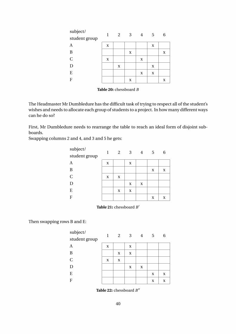
The rook polynomials’ applications are not limited to derangement problems, they coverall sorts of combinatorial problems.Imagine the students of a fictitious school named Hugwarts are given an end of year project.Each project is on a given field of their studies: transfiguration, potions, divination, aston-omy, apparition and defence against the Dark Arts. The students are surveyed on the subjectthey are the least interested in, and then divided into six groups accordingly.
39
subject/
student group1 2 3 4 5 6
A x x
B x x
C x x
D x x
E x x
F x x
Table 20: chessboard B
The Headmaster Mr Dumbledure has the difficult task of trying to respect all of the student’swishes and needs to allocate each group of students to a project. In how many different wayscan he do so?
First, Mr Dumbledure needs to rearrange the table to reach an ideal form of disjoint sub-boards.Swapping columns 2 and 4, and 3 and 5 he gets:
subject/
student group1 2 3 4 5 6
A x x
B x x
C x x
D x x
E x x
F x x
Table 21: chessboard B ′
Then swapping rows B and E:
subject/
student group1 2 3 4 5 6
A x x
B x x
C x x
D x x
E x x
F x x
Table 22: chessboard B ′′
40
x x
x x
x x
x x
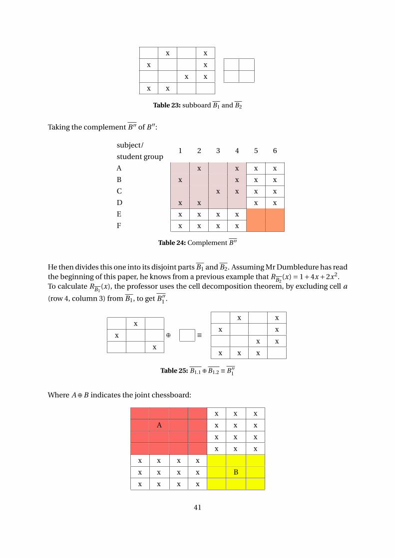
Table 23: subboard B1 and B2
Taking the complement B ′′ of B ′′:
subject/
student group1 2 3 4 5 6
A x x x x
B x x x x
C x x x x
D x x x x
E x x x x
F x x x x
Table 24: Complement B ′′
He then divides this one into its disjoint parts B1 and B2. Assuming Mr Dumbledure has readthe beginning of this paper, he knows from a previous example that RB2
(x) = 1+4x +2x2.To calculate RB1
(x), the professor uses the cell decomposition theorem, by excluding cell a
(row 4, column 3) from B1, to get B ′′1 .
x
x
x
⊕ ≡
x x
x x
x x
x x x
Table 25: B1.1 ⊕B1.2 ≡ B ′′1
Where A⊕B indicates the joint chessboard:
x x x
A x x x
x x x
x x x
x x x x
x x x x B
x x x x
41
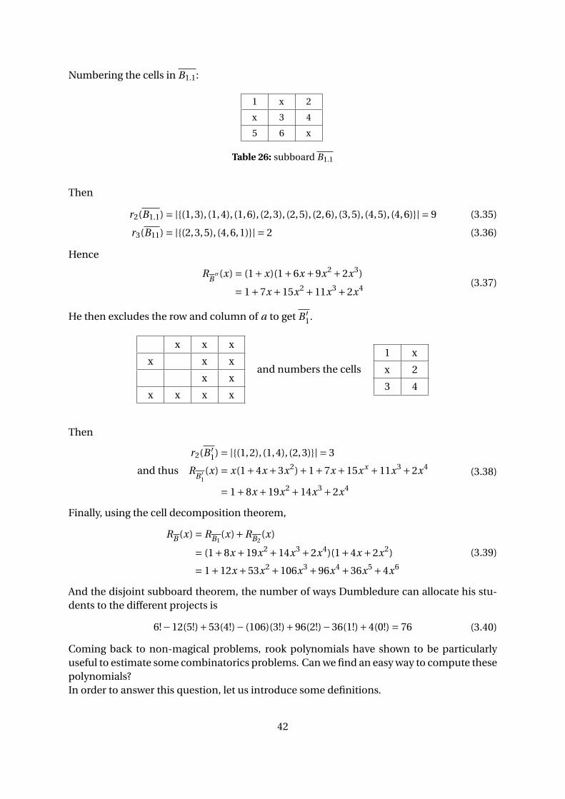
Numbering the cells in B1.1:
1 x 2
x 3 4
5 6 x
Table 26: subboard B1.1
Then
r2(B1.1) = |{(1,3), (1,4), (1,6), (2,3), (2,5), (2,6), (3,5), (4,5), (4,6)}| = 9 (3.35)
r3(B11) = |{(2,3,5), (4,6,1)}| = 2 (3.36)
Hence
RB′′(x) = (1+x)(1+6x +9x2 +2x3)
= 1+7x +15x2 +11x3 +2x4 (3.37)
He then excludes the row and column of a to get B ′1.
x x x
x x x
x x
x x x x
and numbers the cells
1 x
x 2
3 4
Then
r2(B ′1) = |{(1,2), (1,4), (2,3)}| = 3
and thus RB ′
1(x) = x(1+4x +3x2)+1+7x +15xx +11x3 +2x4
= 1+8x +19x2 +14x3 +2x4
(3.38)
Finally, using the cell decomposition theorem,
RB (x) = RB1(x)+RB2
(x)
= (1+8x +19x2 +14x3 +2x4)(1+4x +2x2)
= 1+12x +53x2 +106x3 +96x4 +36x5 +4x6
(3.39)
And the disjoint subboard theorem, the number of ways Dumbledure can allocate his stu-dents to the different projects is
6!−12(5!)+53(4!)− (106)(3!)+96(2!)−36(1!)+4(0!) = 76 (3.40)
Coming back to non-magical problems, rook polynomials have shown to be particularlyuseful to estimate some combinatorics problems. Can we find an easy way to compute thesepolynomials?In order to answer this question, let us introduce some definitions.
42
DEFINITION:The permanent of a n ×n matrix A = (ai j ) is defined as
perm(A) = ∑σ∈Sn
n∏i=1
a i σ(i ) (3.41)
This definition is different from the definition of the determinant of the matrix as we donot take into account the signature of the perutation of the matrix’ elements. Moreover,perm(AB) 6= perm(A)perm(B).Two simple illustrations of the permanent of a matrix are as follows.
perm
(a b cd e fg h i
)= aei +b f g + cdh + ceg +bdi +a f h (3.42)
perm(
1 11 1
)= 1×1+1×1 = 2 (3.43)
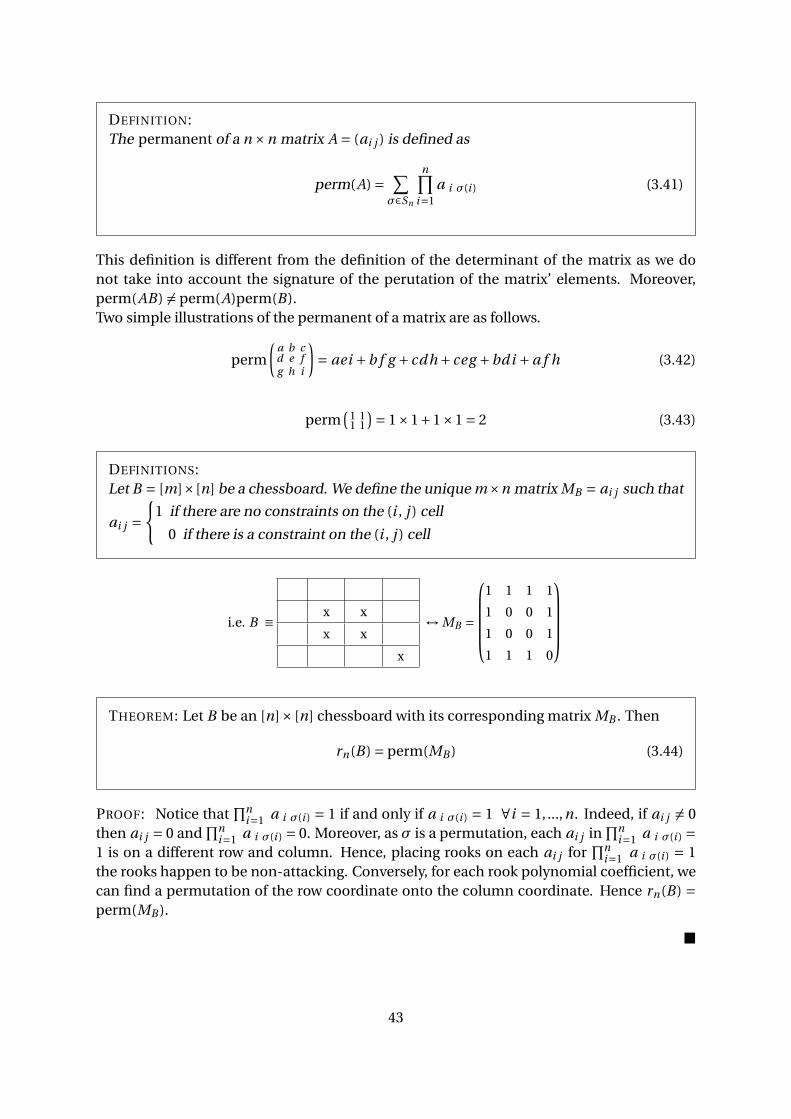
DEFINITIONS:Let B = [m]×[n] be a chessboard. We define the unique m×n matrix MB = ai j such that
ai j ={
1 if there are no constraints on the (i , j ) cell
0 if there is a constraint on the (i , j ) cell
i.e. B ≡ x x
x x
x
↔ MB =
1 1 1 1
1 0 0 1
1 0 0 1
1 1 1 0
THEOREM: Let B be an [n]× [n] chessboard with its corresponding matrix MB . Then
rn(B) = perm(MB ) (3.44)
PROOF: Notice that∏n
i=1 a i σ(i ) = 1 if and only if a i σ(i ) = 1 ∀i = 1, ...,n. Indeed, if ai j 6= 0then ai j = 0 and
∏ni=1 a i σ(i ) = 0. Moreover, as σ is a permutation, each ai j in
∏ni=1 a i σ(i ) =
1 is on a different row and column. Hence, placing rooks on each ai j for∏n
i=1 a i σ(i ) = 1the rooks happen to be non-attacking. Conversely, for each rook polynomial coefficient, wecan find a permutation of the row coordinate onto the column coordinate. Hence rn(B) =perm(MB ).
�
43

3.3.1. Dating app
Consider the new dating app linder, that matches strangers when they both agree on shar-ing their personal information to one-another, based on their profile photos. For instance,when user Tom sees user Zoe’s photo, he decides that user Zoe is a person he is willing todate. Tom will then select ’yes’. Meanwhile, if Zoe sees Tom’s photo and decides that he isworth going out with, she will click on ’yes’ as well: they will have a match, then their contactinformation will be exchanged.However, if Tom sees Zoe’s photo and decides that she is not someone he would like to date,he will select ’no’ and their contact information will not be exchanged.So if any of the two parties rejects the other one, their personal information will remain se-cret. In any case, the profile pictures will be shown to both users, whether they have alreadyaccepted or rejected the other person. In this way the match is unknown until they both hada chance to rate each other.
Now assume that n men and n women have been shown respectively to n women and nmen.
The app developer Zulemberg is experimenting with his creation, and wants to try out a newone-to-one system of dating. This consists on each member being matched to a unique per-son out of everyone they liked, assuming we live in a very fair world and everyone got likedat least once, so that this is a possibility.
The app developer believes that this method will reduce conflicts and unhappiness causedby users matching though not reaching a happy ending. He believes that this one-to-onematching method will increase the percentage of successful relationships. However, he alsobelieves that a random process is necessary, as it is the only one taking into account all thepossible one-to-one matching sets, and we never know who your soul-mate can be. Finally,he reaches the conclusion that he needs to calculate all the possible matching sets and pickone of these sets randomly.Giving it a second thought, Zulemberg encounters the complication of the length of time itwill take him to calculate all possible one-to-one matches.Let us translate this example into rook-polynomial terms. Let B be a chessboard, where thecolumns represent the men’s likes and the rows the women’s likes. If a user rejected anotheruser, then we will consider their intersecting cell as constrained.
44
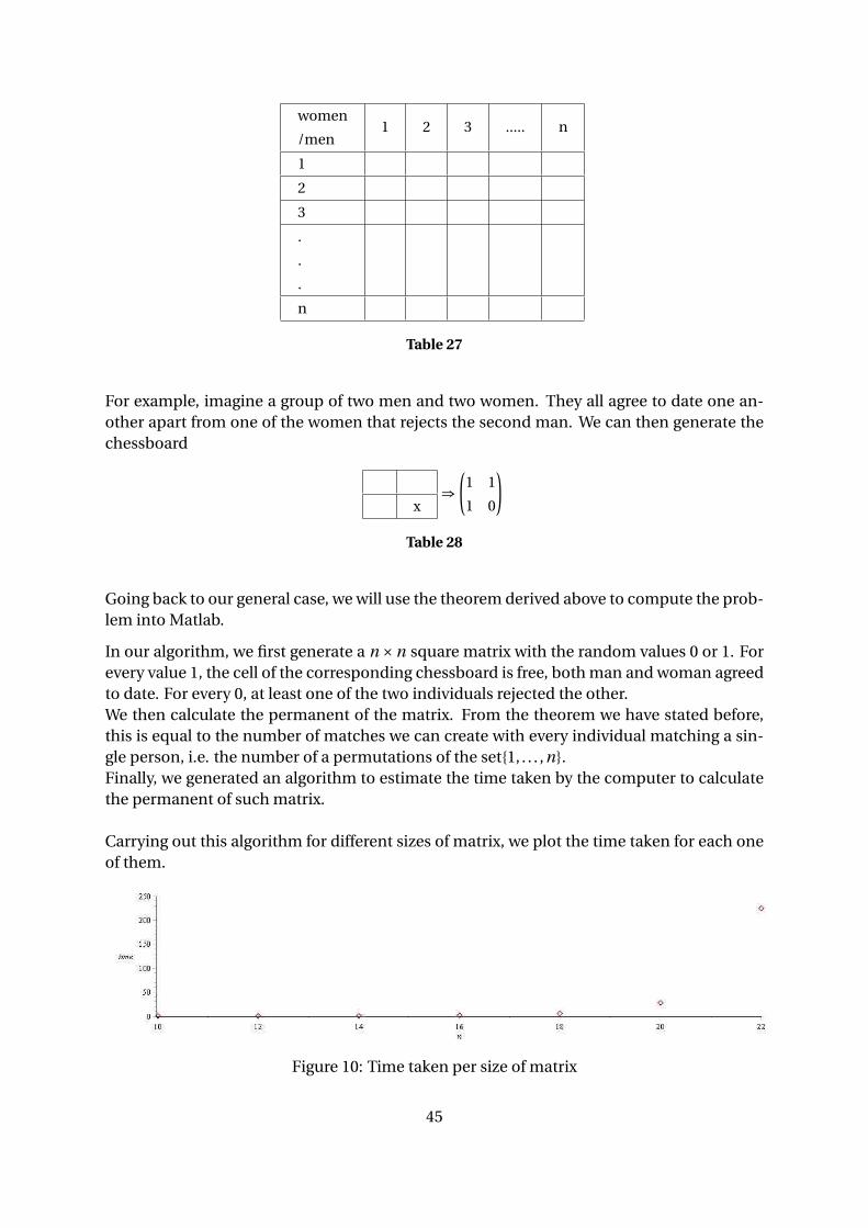
women
/men1 2 3 ..... n
1
2
3
.
.
.
n
Table 27
For example, imagine a group of two men and two women. They all agree to date one an-other apart from one of the women that rejects the second man. We can then generate thechessboard
x⇒
(1 1
1 0
)
Table 28
Going back to our general case, we will use the theorem derived above to compute the prob-lem into Matlab.
In our algorithm, we first generate a n ×n square matrix with the random values 0 or 1. Forevery value 1, the cell of the corresponding chessboard is free, both man and woman agreedto date. For every 0, at least one of the two individuals rejected the other.We then calculate the permanent of the matrix. From the theorem we have stated before,this is equal to the number of matches we can create with every individual matching a sin-gle person, i.e. the number of a permutations of the set{1, . . . ,n}.Finally, we generated an algorithm to estimate the time taken by the computer to calculatethe permanent of such matrix.
Carrying out this algorithm for different sizes of matrix, we plot the time taken for each oneof them.
Figure 10: Time taken per size of matrix
45
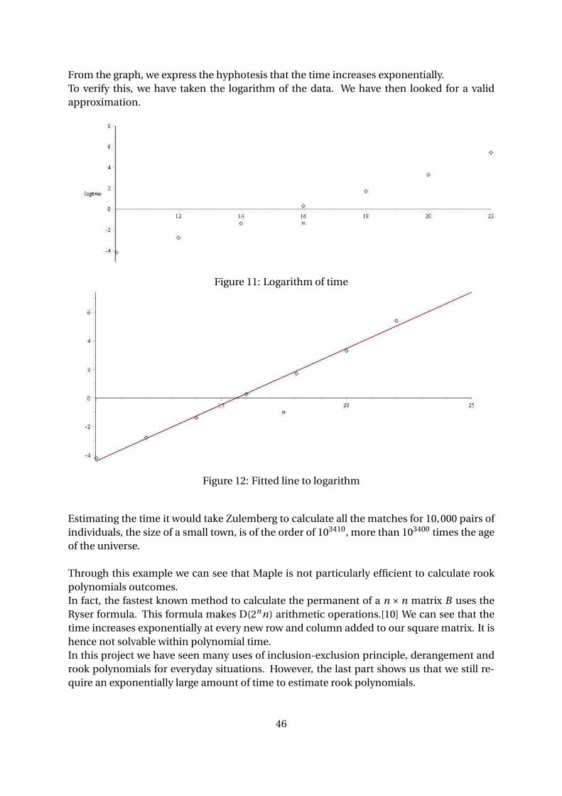
From the graph, we express the hyphotesis that the time increases exponentially.To verify this, we have taken the logarithm of the data. We have then looked for a validapproximation.
Figure 11: Logarithm of time
Figure 12: Fitted line to logarithm
Estimating the time it would take Zulemberg to calculate all the matches for 10,000 pairs ofindividuals, the size of a small town, is of the order of 103410, more than 103400 times the ageof the universe.
Through this example we can see that Maple is not particularly efficient to calculate rookpolynomials outcomes.In fact, the fastest known method to calculate the permanent of a n ×n matrix B uses theRyser formula. This formula makes D(2nn) arithmetic operations.[10] We can see that thetime increases exponentially at every new row and column added to our square matrix. It ishence not solvable within polynomial time.In this project we have seen many uses of inclusion-exclusion principle, derangement androok polynomials for everyday situations. However, the last part shows us that we still re-quire an exponentially large amount of time to estimate rook polynomials.
46
4. Conclusion
The inclusion-exclusion principle is the fundamentals of most of the combinatorics math-ematics that we know. This versatile formula has multiple roots and can be applied in avariety of different ways. Two of the main results derived from the formula are the countingof derangement and the rook polynomials. The derangement counting formula provides aquick solution to count the number of derangements of a set. Eventhough this might seemlike an easy problem to tackle, we have shown that the formula helps us save time in order tofocus on further development of the question examined. However the derangement formulais limited to simple derangement without any additional constraint. In opposition, the rookpolynomial formulation can be too complicated for simple problems like the derangementof a set, but shows its value for complex problems bearing various constraints. Its relationwith matrix permanents enables us to write easy computational algorithms. However, in thelast part of the paper, we showed that even rook polynomials have their limitations.Is it possible to find a polynomial-time algorithm to estimate the combinatorics problemswe have encountered?
5. Bibliography
[1] Gian-Carlo Rota, (1964), On the foundations of combinatoial theory I. Theory of Mobiusfunctions, Zeitschrift fur Wahrscheinlichkeitstheorie 2, 340 - 368.
[2] Alan Tucker, (2012), Applied Combinatorics. 6th edition United States of America, JohnWiley and Sons, Inc.
[3] John Riordan, (1958), An Introduction to Combinatorial Analysis. New York, John Wileyand Sons, Inc.
[4] J.H. van Lint and R.M. Wilson, (1992), A Course in Combinatorics. Cambridge, Cam-bridge University Press.
[5] Roberto Fernandez, Jurg Frohlich, Sokal Alan D., (1992), Random Walks, Critical Phe-nomena, and Triviality in Quantum Field Theory, Texts an Monographs in Physics,Berlin: Springer-Verlag, pp. xviii+444.
[6] A. Bjorklund, T. Husfeldt, M. Koivisto, (2009), Set partitioning via inclusion-exclusion,SIAM Journal on Computing 39 (2): 546-563.
[7] R.B.J.T. Allenby, Alan Slomson, (n.d.), How to Count: An Introduction to Combinatorics:Chapter 17.
[8] V. Longani, (2010), Thai Journal of Mathematics Volumn 8, Number 3, 545-554, Althor-ithm for finding the coefficients of rook polynomials.
[9] Feryal Alayont, Nicholas Krzywonos, (2013), Rook polynomials in three and higher di-mensions, page 36-39.
47

[10] Scott Aaronson, Travis Hance (n.d.) Generalizing and Derandomizing Gurvit’s Approx-imation Algorithm for the Permanent Part 2(19).
48