XuWhite_1996 Shear Wave Velovity

Geophysical Prospecting, 1996, 44, 687-717

A physical model for shear-wave velocitypredictionl

Sh iyu Xu2 and Roy E . Wh i te2

Abstract

The clay-sand mixture model of Xu and White is shown to simulate observedrelationships between S-wave velocity (or transit time), porosity and clay content. Ingeneral, neither S-wave velocity nor S-wave transit time is a linear function ofporosity and clay content. For practical purposes, clay content is approximated byshale volume in well-log applications. In principle, the model can predict S-wavevelocity from lithology and any pair of P-wave velocity, porosity and shale volume.Although the predictions should be the same if all measurements are error free,comparison of predictions with laboratory and logging measurements show thatpredictions using P-wave velocity are the most reliable. The robust relationshipbetween S- and P-wave velocities is due to the fact that both are similarly affected byporosity, clay content and lithology. Moreover, errors in the measured P-wavevelocity are normally smaller than those in porosity and shale volume, both of whichare subject to errors introduced by imperfect models and imperfect parameters whenestimated from logs.

Because the model evaluates the bulk and shear moduli of the dry rock frame by acombination of I(uster and Toksciz' theory and differential effective medium theory,

using pore aspect ratios to characterize the compliances of the sand and claycomponents, the relationship between P- and S-wave velocities is explicit andconsistent. Consequently the model sidesteps problems and assumptions that arisefrom the lack of knowledge of these moduli when applying Gassmann's theory tothis relationship, making it a very flexible tool for investigating how the ?p-"srelationship is affected by lithology, porosity, clay content and water saturation.Numerical results from the model are confirmed by laboratory and logging data anddemonstrate, for example, how the presence of gas has a more pronounced effect onP-wave velocity in shaly sands than in less compliant cleaner sandstones.

In t roduc t i on

Shear-wave velocity logs are essential to the interpretation of amplitude-versus-offset analyses and multicomponent seismic and VSP data. Although the logging

t Paper presented at the 56th EAEG meeting, June 1994, Vienna, Austria.

accepted November 1995.2 Research School of Geological and Geophysical Sciences, Birkbeck and

of London, Malet Street, London \)flC1E 7HX, UK.

e 1996 European Association of Geoscientists & Engineers

Received October 7994, revisron

Uni versity Colleges. Universit l '

687

688 S. Xu and R.E. White

industry now offers a number of S-wave velocity tools, they have been run inrelatively few wells and are still not used routinely. There is therefore a need topredict S-wave velocities from other logs whenever measured S-wave velocity logsare unavailable. Even when an S-wave log has been run, comparison with itsprediction from other logs can be a useful quality control. Prediction can be used tofill gaps in S-wave logs run with, say, monopole sources or to enhance the resolutionof logs from long spacing tools.

A number of empirical laws have been published. These can be divided into fourcategories:

1. zt5 (S-wave velocity) is a linear function of zp (P-wave velocity) as in Castagna'smudrock line (Castagna, Batzle and Eastwood 1985);

2. zts is a linear function of porosity (@) and clay content 2,6 (Tosaya 1982;Castagna et al.1985; Han, Nur and Morgan 1986);

3. S-wave transit time Io is a linear function of porosity and clay content (e.g.Castagna et al.1985);4. shear modulus is a linear function of porosity (e.g. Blangy and Nur 1992).

In general empirical models are simple and straightforward. Some empiricalrelationships, like the time-average equation and Archie's law, are still widely usedin the oil industry today.

The disadvantages of empirical relationships are:1. they tell us very little about the physical mechanisms of rock properties;2. a large quantity of data and detailed analysis are needed to establish a reliable

relation;3. their conditions of validity may nor be well defined.

It is therefore useful to have a physical model that provides some understanding ofS-wave behaviour. If an S-wave sonic log is available, such a model may helpgeophysicists, log analysts or petrophysicists interpret the measurements.

Greenberg and Castagna (1992) developed a semiphysical model in order topredict S-wave velocity in porous rocks. The authors employed an empiricalrelationship to relate S-wave velocity to compressional velocity in fully brine-saturated rocks. Wood's (1941) suspension model was used to average the bulkmodulus of pore fluids if partially saturated, and the Voigt-Reuss-Hill (\fang andNur 1992) equation was used to estimate mixed grain incompressibility. Applicationsof the Greenberg and Castagna (1992) model to both laboratory measurements andlogging data show that S-wave velocity can be estimated with a precision of betterthanTo/o. The success of the model was attributed to the robust relationship betweenP-wave and S-wave velocities but there was no physical model of the relationshipitself.

Xu and White (1995a) proposed a clay-sand mixture model based on the Kusterand Toksciz (1974), Gassmann (1951) and differential effective medium (DEM)theories, which related P-wave velocity in sand-shale systems to porosity and claycontent. The applicability of the model was confirmed by comparing its predictionswith laboratory measurements and sonic logs recorded over depth intervals where

A 1996 European Association of Geoscientists & Engineers, Geophgsical Prospecting, 44, 687-717

A physical model for s-waae aelocity prediction 689

formations varied from unconsolidated and uncemented to consolidated sand-shalesequences (Xu and !7hite 1995a).

This paper demonstrates that the clay-sand mixture model can predict S-wave

velocity in siliciclastic rocks as well as or better than P-wave velocity. $7e begin witha review of the model and then demonstrate how the model simulates observed

relationships between S-wave velocity and porosity and clay content. The modelthus provides a basis for predicting S-wave velocity from rock parameters or fromother logs. It is applied to the laboratory measurements of Rafavich, Kendall andTodd (1984) and Han et al. (1986) and to two sets of S-wave and other log dataprovided by BP. Finally, the effects of clays and water saturation on the apf vs ratio

are investigated.

The c lay-sand mixture model

The clay-sand mixture model (Xu and \X/hite 1995a) is a physical model forvelocities in siliciclastic rocks developed from the Kuster-Tokscjz (1974), DEM(Bruner 1976; Cheng and Toksciz 1979) and Gassmann (1951) theories. The modelhas two key features. The first is that it characterizes the compliances of the sand and

clay mineral fractions of the rock by assigning to them separate pore spaces having

different effective pore aspect ratios (ratios of short semi-axis to long semi-axis). The

second key feature is the use of Kuster and Toksciz (1974) and DEM theories to

compute the elastic moduli of the dry frame. Given the dry frame moduli, application

of Gassmann's (1951) equations then gives the low-frequency velocity in the fluid-

saturated rock.The inputs required by the model comprise the densities and elastic moduli of the

sand grains, clay particles and the pore fluid, the porosity and clay content ofthe rock

frame, and two aspect ratios, one (ar) for pores associated with sand grains and one

(cv.) for pores associated with clay minerals (including bound water). Shale volume

replaces clay content in well-log applications. Details of how these parameters are

determined is included with the discussion of practical examples but, apart from the

aspect ratios, they come from tabulated values and log or laboratory measurements.

The aspect ratios cannot be measured directly and their estimation relies on a best fit

to 1og or laboratory observations. All results to date show that o, is close to 0.1 and a.is of the order of 0.03. Xu and White (1995a, Fig. 1) give a flow chart showinghow P-wave and S-wave transit times (strictly slownesses, reciprocals of velocities)are constructed from these inputs.

The use of two aspect ratios to describe the hypothesized different pore spaces

associated with the sand and clay mineral fractions of the rock is obviously a gross

simplification. A model with two aspect-ratio distributions may be more plausible

but the need to specify the parameters of such distributions makes this option utterlyimpractical. In fact a single aspect ratio can simulate the elastic response of a uniformdistribution of pores rather well (M. Sams, pers. comm.). As logs give no informationon the pore volumes related to sand grains and to clays, we compute these on the

O 1996 European Association of Geoscientists & Engineers, Geophysical Prospecting, 44, 687-717

690 S. Xu rsrd R.E. White

5.6

5.4

5.2

5.0

4.8

4.6

4.4

xs*\<A

\')

\)

=I

-- Voigt-'- Spheres (KT). . . . HSboundave rage---. Voigt-Reuss-Hill- Time Average". . . . . Renss

0.0 0.2 0.4 0.6 0.8 1 .0

Shale volume (fractional)Figure 1. Comparison of P-wave velocities of the sand grain and clay particle mixtureestimated using various averaging schemes. P-wave, S-wave velocities and density of the sandgrain used in this simulation are 5.86km/s,3.9lkm/s and 2650kg/m3, and those for clayparticles are 4.45 km/s, 2.54 km/s and 2600 kg/m3.

assumption that, to a first-order approximation, they are proportional to sand-grainvolume and clay content (see Appendix; the fractional sand volume is obtained bysubtracting the total porosity and fractional clay volume from one).

In order to apply Kuster and Toksciz' (1974) theory to computation of the elasticproperties of the dry frame, we need the bulk and shear moduli of the mixture of sandgrains and clay minerals. There are several averaging schemes available in theliterature which can be used to approximate the effective elastic constants of the grainmixtures. Figure 1 shows numerical results from some commonly used schemesdescribed by wang and Nur (1992). As this figure shows, the voigt scheme providesan upper bound while the Reuss scheme provides a lower bound; the Kuster andToksciz (1974) formulation for spheres is nearly identical to the Hashin-shtrikmanupper bound, the time-average approximation is very close to the Hashin-shtrikmanlower bound (the bounds are not plorted to avoid crowding the diagram further)while the voigt-Reuss-Hill average scheme and the Hashin*Shtrikman boundaverage fall between the time-average and the Kuster and Toksciz (1974)approximation for spheres.

Apart from the Voigt and Reuss schemes, there is little to choose between theproposed schemes. The reason for this lies in the low velocity contrast between

e) 1996 European Association of Geoscientists & Engineers, Geophysical Prospecting,44,687-7I7


different grain minerals. We used time-average equations to compute P- and S-wavetransit times of the grain mixture because we believe they provide a simple and closeapproximation to the low-frequency conditions that mainly concern us. The elasticbulk and shear moduli of the mixture are then calculated from its P- and S-wavetransit times and density. The equations for these and subsequent calculations aregiven in the Appendix.

The moduli of the dry rock frame are calculated from Kuster and Toksciz' (1974)equations for evaluating the moduli of an elastic medium permeated with a dilute(d << ") distribution of empty randomly oriented non-interacting ellipsoidal pores.We overcome the limitation on porosity by applying DEM theory (Xu and \X/hite1995a), introducing the pores in steps) each step injecting a concentration smallenough to satisfy the condition S < a. The effective elastic moduli are updated usingKuster and Toksciz' (1974) equations and the updated moduli input to the next step,the process being repeated until the total porosity is reached.

In order to model transit t imes or velocities of low-frequency P- and S-waves, themoduli of the dry rock frame are input to the Gassmann ( 195 1) model to simulate theeffect of fluid relaxation. To model propagation at high frequencies, we dispense withGassmann's (1951) theory and calculate the effective elastic moduli of the saturatedrock by including the bulk modulus of the pore-fluid inclusions when applying theKuster and Toksciz (1974) and DEM theories. This procedure assumes that fluidflow is the prime cause of velocity dispersion in rocks. It is based on the resultsof Mavko and Jizba (1991) and Mukerji and Mavko (1994) which show thatGassmann's (1951) equations are a low-frequency approximation whereas thetheories of Hudson (1981) and I{uster and Tokscjz (1974) which assume isolatedpores are high-frequency approximations. In applying Kuster and Toksciz (1974)

theory to derive the elastic moduli of dry rock frame, it does not matter whether thepores are connected or isolated because they are empty. In terms of the fluid-flowmechanisms, the subsequent application of Gassmann's (1951) theory makes thisversion of the model a low-frequency one) applicable to seismic modelling andpossibly well-log analysis. In the high-frequency version of the model, there is nofluid flow between pores corresponding to only local stress relaxation inside eachpore.

Our previous paper (Xu and Vhite 1995a) demonstrated, using well logs andpublished laboratory measurements, how predictions from the clay-sand modelexplain much of the scatter commonly seen in porosity-velocity (P-wave) cross-plotsfrom siliciclastic rocks. The model also simulates the two distinct porosity-velocity

trends observed by Marion et al. (1992) for shaly sands and for sandy shales.Recently (Xu and \7hite 1995b), we demonstrated that, whereas the low frequencywas suitable for modelling logging data, the high-frequency model was more suitablefor simulating laboratory measurements made at frequencies from hundreds of KHzto MHz. $7e use the appropriate version of the model in the comparisons ofpredictions and observations that follow.

We have also extended the model to simulate the anisotropic behaviour of shales

O 1996EuropeanAssociat ionofGeoscient is ts&Engineers, GeophysicalProspect ing,44,6ST-717

692 S. Xu and R.E. IVhite

and sandy shales (Xu and White 1995c) by including an orientation distribution forpores associated with clays, similar to that proposed Hornby, Schwartz and Hudson(1994) for modelling pure shales. Details are left for a subsequent publication.

Preliminary results show that the velocity behaviour of elastic waves travelling in

directions perpendicular to the preferred orientation of the pores is close to thatpredicted by the isotropic model. The assumption of random orientation cannot bejustified for clay-related pores and predictions from the isotropic model are intendedfor the vertical direction only.

The prediction of S-wave velocities in siliciclastic rocks is a natural extension ofthe model. Moreover prediction of S-wave velocity t;s requires the estimation of noparameters beyond those already employed in zp prediction and achieves as good orbetter practical accuracy.

S-wave veloc i ty and P-wave veloc i ty , porosi ty and c lay content

Results from laboratory measurelnents

Figure 2 shows measurements, made by Han et al. (1.986) at 40MPa confiningpressure and 1 MPa pore pressure, that demonstrate how S-wave velocity decreaseswith porosity and clay content. There is indeed much laboratory evidence (e.g.

4.0

3.5

3.0

2.5

D

0.0 0.1 0.2 0.3

Porosity (fractional)

Figure 2. Illustration of the observed variation of S-wave velocity with porosity and claycontent. Different symbols represent different volume fractions of clay content. Measurementsare from Han et al. (1986).

O 1996 European Association of Geoscientists & Engineers, Geophysical Prospecting, 44,687-717

2.

. l -

-v

-U

u\)

3I

v1

A

a8

1.5

A physical modelfor s-waae aelocity prediction 693

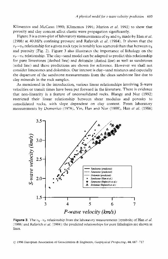
Klimentos and McCann 1990; Klimentos 1991; Marion et al. 1992) to show thatporosity and clay content affect elastic wave propagation significantly.

Figure 3 is a cross-plot of laboratory measurements of zp and zs made by Han et al.(1986) at 40MPa confining pressure and Rafavich et al. (1984). It shows that the?rp-?s relationship for a given rock type is notably less scattered than that between agand porosity (Fig. 2). Figure 3 also illustrates the importance of lithology on the"p-"s relationship. The clay-sand model can be adapted to predict this relationshipfor pure limestones (dashed line) and dolomite (dotted line) as well as sandstones(solid line) and these predictions are shown for reference. However we shall notconsider limestones and dolomites. Our interest is clay-sand mixtures and especiallythe departure of the sandstone measurements from the clean sandstone line due toclay minerals in the rock samples.

As mentioned in the introduction, various linear relationships involving S-wavevelocities or transit times have been put forward in the literature. There is evidencethat non-linearity is a feature of unconsolidated rocks. Blangy and Nur (1992)

restricted their linear relationship between shear modulus and porosity toconsolidated rocks, with slope dependent on clay content. From laboratorymeasurements by Domenico (1976), Yin, Han and Nur (1988), Han et al. (1986)

3.0

2.5

2.0

- Sudsane (predicted)- - - Lircstone (predbted)'..... Doloilite (predicted)

. Sandstue (H6 et al.)$ Lircsrone (Rgnich et ol.)A Dobmite (R60ich et al.)

P-wave velocity (km/s)Figure 3. The z5-z;p relationship from the laboratory measurements (symbols) of Han et al.(1986) and Rafavich et al. (1984); the predicted relationships for pure lithologies are shown asl ines.

(A 91996 European Association of Geoscientists & Engineers, Geophgsical Prospecting, 44,681-777

s*\a

h

\)

q)

3I

4


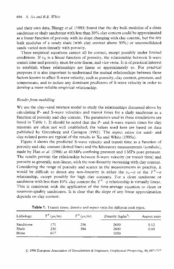
and their own data, Blangy et al. (1993) found that the dry bulk modulus of a clean

sandstone or shaly sandstone with less than 30% clay content could be approximatedas a linear function of porosity with its slope changing with clay content, but the drybulk modulus of a sandy shale (with clay content above 307o) or unconsolidatedsands varied non-linearly with porosity.

These empirical equations cannot all be correct, except possibly under limitedconditions. If os is a linear function of porosity, the relationship between S-wavetransit time and porosity must be non-linear, and vice versa. It is of practical interestto establish where relationships are linear or approximately so. For practicalpurposes it is also important to understand the mutual relationships between thosefactors known to affect S-wave velocity, such as porosity, clay content, pressure, andtemperature, and to isolate any dominant predictors of S-wave velocity in order todevelop a more reliable empirical relationship.

Results from modelling

rJfe use the clay-sand mixture model to study the relationships discussed above bycalculating P- and S-wave velocities and transit times for a shaly sandstone as afunction of porosity and clay content. The parameters used in these simulations arelisted in Table 1. It should be noted that the P- and S-wave transit times for clayminerals are often not well established; the values used here are based on datapublished by Greenberg and Castagna (1992). The aspect ratios for sand- andclay-related pores are typical of the results in Xu and \7hite (1995a).

Figure 4 shows the predicted S-wave velocity and transit time as a function ofporosity and clay content (dotted lines) and the laboratory measurements (symbols),made by Han et al . (1986) at 40 MPa confining pressure and I MPa pore pressure.The results portray the relationship between S-wave velocity (or transit time) andporosity as generally non-linear, with the non-linearity increasing with clay content.Considering the range of porosity and scatter in the measurements in practice, itwould be diff icult to detect any non-linearity in either the as-Q or the 7s-/relationship, except possibly for high clay contents. For a clean sandstone orsandstone with less than 10% clay content the Is-@ relationship is virtually linear.This is consistent with the application of the time-average equation to clean orreservoir-quality sandstones. It is clear that the slope of any linear approximationdepends on clay content.

Table 1 . Transit times, density and aspect ratio for different rock types.

Lithology .r - ( trslm) 7s (pslm) Density (kg/m') Aspect ratio

SandstoneShaleBrine

1712306 t 7

256394

265026001050

o . t 20.03


3.5

3.0

2.5

2.0

1.5

I

x*54

>.

v

v

3I

V)

A physical model for s-zoaz,e aelocity prediction 695

0.1 0.2 0.3


r19.... . 4

!.

4 t 4

rl. '

a t .

:

\)

q

P

u

3q

Vc=SOVo.:' ....

o .$ . . ' . . '

. ' . ; ; l t

" o ' S. . : . * . . , . . 4

:r:.slsi tt;' ' . . ' . . o ? . . . t r "+ci.. s .. " ... d

. A - . . . 4

. . " '

d ' '

0.0 0.1 0.2 0.3


Figure 4. (a) S-wave velocity and (b) S-wave transit time as a function of porosity and claycontent, caiculated using the clay-sand mixture model (dotted lines). The various symbolsrepresent the measurements of }{an et al. (1986) at 40MPa confining pressure for variousvolume fractions of clay content. Model parameters are listed in Table 1.

These results suggest that linearity may be a reasonable approximation when theclay content is less than, say,3Ooh but that it is not applicable when both porosity

and clay content are significantly high. Of course the model must accord with

observations for these conclusions to be valid but comparison of the measurementsand the predictions shows that the model is simulating laboratory observations rather



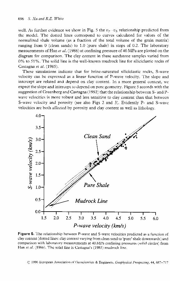
well. As further evidence we show in Fig. 5 the z'p-25 relationship predicted fromthe model. The dotted lines correspond to curves calculated for values of thenormalized shale volume (as a fraction of the total volume of the grain matrix)ranging from 0 (clean sands) to 1.0 (pure shale) in steps of 0.2. The laboratorymeasurements of Han et al. (7986) at confining pressure of 40 MPa are plotted on thediagram for comparison. The clay content in these sandstone samples varied from0o/o to 51o/". The solid line is the well-known mudrock line for siliciclastic rocks ofCastagna et a l .119851.

These simulations indicate that for brine-saturated siliciclastic rocks, S-wavevelocity can be expressed as a linear function of P*wave velocity. The slope andintercept are related and depend on clay content. In a more general context) weexpect the slope and intercept to depend on pore geometry. Figure 5 accords with thesuggestion of Greenberg and Castagna (1992) that the relationship between S- and P-wave velocities is more robust and less sensitive to clay content than that betweenS-wave velocity and porosity (see also Figs 2 and 3). Evidently P- and S-wavevelocities are both afected by porosity and clay content as well as lithology.

Shale

Mudrock Line

2.5 3.0 3.5 4.0 4.s

P-wave velocity (km/s)

Figure 5. The relationship between P-wave and S-wave velocities predicted as a function ofclay content (dotted lines: clay content varying from clean sand to 'pure' shale downwards) andcomparison with laboratory measurements at 40 MPa confining pressures (solid circles) fromHan et al. (1986). The solid line is Castagna's (1985) mudrock line.

4@1996 EuropeanAssociationofGeoscientists&Engineers, GeophysicalProspecting,44,68T-717

4.0

CleanI\\I

. t

Sandx-\c>.

q)

\)

iIv2

" \

Pure

3.0

2.5

2.0

1.5

1.0

6.05.55.02.0


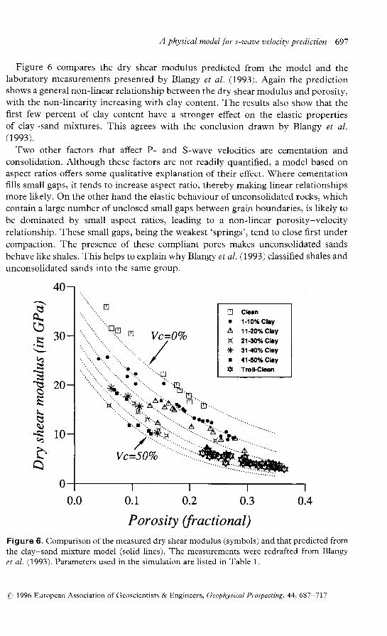
Figure 6 compares the dry shear modulus predicted from the model and thelaboratory measurements presented by Blangy et al. (1993). Again the predictionshows a general non-linear relationship between the dry shear modulus and porosity,with the non-linearity increasing with clay content. The results also show that thefirst few percent of clay content have a stronger effect on the elastic propertiesof clay-sand mixtures. This agrees with the conclusion drawn by Blangy et al.(1993).

Two other factors that affect P- and S-wave velocities are cementation andconsolidation. Although these factors are not readily quantified, a model based onaspect ratios o{Iers some qualitative explanation of their effect. \rhere cementationfi.lls small gaps, it tends to increase aspect ratio, thereby making linear relationshipsmore likely. On the other hand the elastic behaviour of unconsolidated rocks, whichcontain a large number of unclosed small gaps between grain boundaries, is likely tobe dominated by small aspect ratios, leading to a non-linear porosity-velocity

relationship. These small gaps, being the weakest 'springs', tend to close first under

compaction. The presence of these compliant pores makes unconsolidated sandsbehave like shales. This helps to explain why Blangy et al. (1993) classified shales andunconsolidated sands into the same group.

40

U CLan. 1-10% ClayA 11-2096ctayX 21{0%Clay

* 3l{!%Glayr 41-5095 Clayg Troll-Cloan

b

0.0 0.1 0.2 0.3 0.4

13trr \: 3 0

4

s\ 2 0

\J

ss\J

E 1 0ho

0

Porosity (fractional)Figure 6. Comparison of the measured dry shear modulus (symbols) and that predicted fromthe clay-sand mixture model (solid lines). The measurements were redrafted from Blangyet al. (1993\. Parameters used in the simulation are listed in Table 1.

O 1996 European Association of Geoscientists & Engineers, Geophysical Prospecting,44,687-717


Shear-wave veloc i ty predict ion

Procedure

The model can predict S-wave velocity using measurements of1. grain matrix parameters (lithology), porosity and clay content (Fig. 4),2. lithology, P-wave velocity and clay content (Fig. 5), or3. lithology, P-wave velocity and porosity (Xu and White 1995b).

If all the measurements are error free, it does not matter which scheme is used. Inpractice schemes 2 or 3 should be used because(a) there is a very good correlation between ?rp and zs: both are similarly affected byporosity, clay content and lithology; and(b) the sonic log is usually more reliable than estimates of porosity and shale volumefor which errors) besides those involved in the measurementsr may be introduced dueto the use of imperfect models and imperfect parameters.Xu and \7hite (1995b) illustrate how comparison of the S-wave logspredicted from schemes 2 and 3 helps check the consistency of the model andidentify unreliable portions of log. Here we confine ourselves to the use ofscheme 2.

Figure 5 provides the basis for scheme 2. It shows that S-wave velocity can bepredicted from P-wave velocity and clay content. This does not mean that S-wavevelocity is independent of porosity. Rather the P-wave velocity contains all theinformation about porosity needed to predict S-wave velocity.

Figure 5 also shows to what degree our model can improve the ?rsprediction over Castagna's (1985) mudrock line. For P-wave velocities, sayhigher than 4.5 kmis, the maximum correction is less than 87o and there islittle advantage over Castagna's (1985) mudrock line unless the errors in P-wave velocity are some fraction of this (the fraction depends on the accuracyof the clay content). On the other hand, for low P-wave velocities (highporosities), the improvement may be significant, depending on the variations in claycontent.

C omp arison with labor atory measur ernents

We use the laboratory measurements made by Han et al. (1986) at 5 MPa confiningpressure and l MPa pore pressure to study the validity of the model. Figure 7 showscross-plots of the measured and predicted S-wave velocities using (a) porosity andclay content and (b) P-wave velocity and clay content. The smaller scatter in Fig. 7bconfirms the robust relationship between P- and S-wave velocities stated above andindicates the degree of improvement obtained from the model. Parameters used inthe S-wave prediction are listed in Table I except that the best-fit aspect rarios were0.08 for sand-related pores and 0.02 for clay-related pores. These lower values can beattributed to the reduced effective pressure which allows pores with low aspect ratios,

e 1996 European Association of Geoscientists & Engineers, Geophgsical Prospecting,44,687-717

1.0

A physical model for s-wave aelocity prediction 699

(a) Predictedfrom porosiry and clay content

l.s 2.0 2.5 3.0 3.s

r 1.5 2.O 2.5 3.0 3

Measured S-wave velocity (lon/s)

(b) Predictedfrom P-wave velacity and clay content

1.0 1.5 2.0 2.5 3.0 3.5r3.5

3.5

2.5

2.0

sa>\

q)

3Ir'')

3.0

1.5

2.0

2.

2.

l .

1

1.5

x"\a

A

A

\)

3q

L

J 1 . 03.51.0 1.5 2.0 2.5 3.0

Measured S-wave velocity (lon/s)

Figure 7. Cross-plot of measured S-wave velocities against predictions from (a) porosity and

clay content and (b) P-wave velocity and clay content. The measurements were made from 75

samples at 5 MPa conflning pressure by Han et al. (1986).

or cracks, to remain openJ thereby reducing the mean aspect ratios for sand-

and clay-related pores. The best-fit aspect ratios for modelling the measure-

ments at 40MPa confining pressure (Han et al. 1986) were the same as those

tabulated in Table 1. The results at 5 MPa are more scattered than those at

40 MPa, presumably because of microcracks, and make a sterner test of the

model.

O 1996 European Association of Geoscientists & Engineers, Geophysical Prospecting' 44,687-717


Comparison with log data

\7e also applied the model to P- and S-wave logs from two wells provided by BP.Before giving results, we discuss how to determine the required parameters fromwell-log analysts and how they affect velocity predictions.

Guidelines for par amet er det ermination

Published data (e.g. Serra 1984, p.225) show very l itt le variation in densities, P-and S-wave transit times for brine and for lithologies without porosity such astight sandstone, limestone and dolomite. Although factors such as cementation,temperature, pressure, etc.r may affect these parameters, the effects are relativelysmall in comparison with other factors described below. (It is possible to classifycement as a lithology, but we do not do it because it is hard to identify cement typeand cement volume from a normal log analysis). The parameters for sand grains andbrine are therefore based on published tables. Values for oil and gas can also be foundfrom tables but must be corrected for temperature and pressure.

The parameters for the clay particles must be checked for consistency with thelogs. First of all there are few published values for the P- and S-wave velocities anddensities of different clay minerals. Secondly, in practical formation evaluation, loganalysts normally evaluate shale volume instead of clay content and there are anumber of problems in determining shale volume.

1. It is often uncertain what types of clay minerals the shale contains.2. Shale consists of silts as well as clay minerals and the volume of the silts can, on

occasion, be more than 50% of the total volume.3. Shale, however pure it is, contains a certain amount of bound water and/or

hydration water.4. A 'pure' shale defined by gamma-ray or other logs may be overpressured or

poorly compacted; it is likely to contain some residual porosity.5. changes in hole size can alter the response of the gamma-ray tool, making it

difficult to ensure consistent estimation of shale volume over different log intervals.6. Different relationships have been proposed for converting gamma-ray readings

into shale volumel we generally use the non-linear relationship of Rider (1991, p.66)for pre-Tertiary consolidated rocks.Given these uncertainties, which are by no means atypical of log analysis in shalyintervals, estimation of shale parameters has to rely on careful assessment of the logsand is better illustrated by example than by proposing an artificial .cut-and-dried'

procedure. These uncertainties are compounded by the strong coupling between theparameters adopted for the shale and the clay-related aspect ratior although thecoupling does not greatly hamper os prediction in practice.

In many wells parameters for a 'pure' shale can be found on the gamma-ray logfrom a deep well-compacted shale. This was so in case study 1 below, whichillustrates how the shale parameters can be estimated. The parameters from a .pure'

O 1996EuropeanAssociat ionofGeoscient is ts&Engineers, GeophysicalProspect ing,44,6ST-717

A phjtsical model for s-waae aelocity prediction 701

shale zone defined from the gamma-ray log at depths around 2895 m in Well A of thiscase study are listed in Table 2.The table also lists the density and P-wave transittime of a well-compacted shale in well 44129-lA in the southern North Sea (Xu andlfhite 1995a). These values are close to those given by Greenberg and Castagna(1992) for illite and a corresponding value for the S-wave transit time was assigned tothis shale on the basis of this similarity. Although they may change from area to areaor even from well to well, such tabulated shale parameters are a useful guide for

deciding whether a selected 'pure' shale zone contains significant residual porosity.

The relatively high P-wave transit time and low density at Well A suggest that a

certain amount of residual porosity is present. The values are consistent with the

assumption that the residual porosity for this shale zone is about lloh and the P-wave

transit time and density for the corresponding 'pure' shale without residual porosity

are 230prs/m and 2600kg/m'. By correcting the gamma-ray and neutron logs for

this 1 1% porosity, corrected log values for the shale without residual porosity can

be obtained (see Table 2). In summary the shale parameters were estimated by

trial-and-error calculations using comparable tabulated and field parameters.

There are two options for choosing shale parameters for velocity prediction in this

example: (1) using original log values and (2) using corrected log values. The former

are compromised by any residual porosity and the latter by uncertainties in the

correction. As the presence of porosity makes the shale appear more compliant than

its clay minerals really are, the model requires a larger (less compliant) aspect ratio

than one with the correct shale parameters. Nevertheless use of the original log values

gave a slightly better fit in case study 1.

Porosity is evaluated by a standard method using the Well Data System log

analysis package. A reliable estimate of porosity is important to the method and as

many logs as are available are used. A density log is essential and a neutron porosity

log over at least some interval; deep resistivity logs, which are generally run, can also

provide estimates of porosity where brine properties are known. The best check is

comparison of the porosity log with core measurements. Given a reliable porosity

log, it is possible to compute a pseudoshale-volume log from the P-wave transit

times (Xu and \flhite 1995b) and this can be helpful in identifying problems in the

shale-volume estimates.

Table 2. Log values ofa'pure' shale before and after correction for efectiveoorositv.

Log type (Unit)Log values Log values

(beforecorrection) (aftercorrection)

GRRHOBNPHIDT (P-wave)DT (S-wave)

(API)(ke/m3)

(pslm)(s,Vm)

982450

0.45341689

1082600

0.40230394

O 1996 European Association of Geoscientists & Engineers, Geophysical Prospecting,44' 681-777


Panel 5 Pmel6

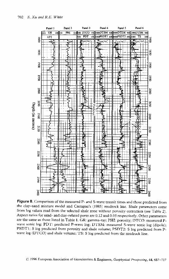
Figure 8' Comparison of the measured P- and S-wave transit times and those predicted fromthe clay-sand mixture model and Castagna's (1985) mudrock line. Shale paramerers comefrom log values read from the selected shale zone without porosity correction (see Table 2).Aspect ratios for sand- and clay-related pores are 0.12 and 0.05 respectively. Other parametersare the same as those listed in Table l. GR: gamma-ray; PHI: porosity; DTCo: measured p-wave sonic log; PDT: predicted P-wave log; DTSM: measured s-wave sonic log (dipole);PSDTI; s log predicted from porosity and shale volume; pSDT2: s log predicted from p-wave log (DTCO) and shale volume; TS: S log predicted from the mudrock line.

N

N

I

N

V 8

A N

t!

( D p

NN

5

Np


A physical model for s-waae ztelocity prediction

Pmel 3 Pmel4 Pmel 5 Pmel 6

703

Pmel I Pmel2

p

-

!a

p

-

p

N6

I

v ! 4

a a5 X

(|O p

p

8

p

pI

I

p

O

5

Figure 8. Continued

i ( l ) l996EuropeanAssociat ionofGeoscient is ts&Engineers, GeophysicalProspect ing,44'687-717


Panel 1 Panel 2 Panel 3 Panel 4 Panel 5 Panel 6

Figure 9. Comparison of the measured P- and S-wave transit times and those predicted fromthe clay-sand mixture model and Castagna's (1985) mudrock line. Shale parameters comefrom log values corrected for the residual porosity contained in the selected shale zone (seeTable 2). Aspect ratios for sand- and clay-related pores are 0.12 and 0.03, respectively. Otherparameters are the same as those listed in Table 1. Notations are the same as those for Fie. 8.

H

o

o

.c) 1996 European Association of Geoscientists & Engineers, Geophysical Prospecting, 44, 687-717

A physical model for s-wave aelocity prediction

Panel 3 Panel 4 Panel 5 Panel 6

705

Panel I Panel 2

N)

8

p5

t\)

I

p

f-)

I

t..): o \

6 o

a q! r i

o( D N )@ {

l'Ja

8

N*

N

8

NJ

o

8

Figure 9. Continued

qt 1996 European Association of Geoscientists & Engineers, Geophysical Prospecting) 44' 687-717


Once the porosity has been evaluated and the shale parameters chosen, the

estimation of aspect ratios is relatively straightforward since it simply relies onmaking a best fit. Vith just two parameters to be estimated, the procedure could bereadily automated. However we prefer a visual approach that can take account ofspecific problems in the logs and concentrate on sandy intervals when tuning agguided by the normalized mean-square error (NMSE, Xu and \X/hite 1995a) betweenthe observed and predicted logs. Trials to date have consistently yielded aspect ratiosclose to 0.10 for the sand component and around 0.02-0.05 for the clay component.We noted above that the best-fit aspect ratio for clay-related pores depends on howthe 'pure' shale zone was selected.

Although it would be helpful to have independent estimates of the effective aspectratios of sand-related and clay-related pores, there is no ready way of obtaining them.The aspect ratios employed by the model characterize the elastic behaviour of the twosolid components and their differing response to porosity. In effect the model uses abimodal distribution of pores, with concentrations determined by the normalizedsand volume and clay content. $Thatever its defects in the abstract, the model hasbeen tried in blind tests and succeeded just as well in predicting r,5 in these as in thetwo case studies reported below. Given a sufficient base of well data, it may bepossible to relate aspect ratios to other parameters such as effective pressure.

Case 1: Well A

Figure 8 shows a comparison of the measured P- and S-wave sonic logs at this wellwith the model predictions using 'pure' shale parameters directly read from logs atthe selected shale zone. Figure 9 shows the comparison with predictions usingcorrected shale parameters. The same parameters for sand grains and pore fluid(Table 1) are applied in both cases. The gamma-ray log is presented in panel 1 andthe porosity log estimated from the density log is shown in Panel 2.Pane|3 comparesthe measured P-wave transit times (DTCo) and those predicted from our model(PDT). Panels 4 to 6 show the comparisons between the measured S-wave transittimes and those predicted from porosity and shale volume (pSDTl in panel 4), fromP-wave transit time (DTCo) and shale volume (pSDT2 in panel 5) and fromCastagna's (1985) mudrock l ine (TS in Panel 6).

The two figures illustrate some important points.1' Prediction of S-wave velocity from P-wave velocity and shale volume is more

reliable than prediction from porosity and shale volume. The reasons for this wereexplained in the previous section.

2. Castagna's (1985) mudrock line works well for shaly formations with less than20%o porosity but underestimates transit times when the porosity exceeds 207o(NMSE : O.ll7). This accords with the results shown in Fig. 5.

3. The aspect ratio for sand-related pores is stable at 0.12 but the aspect ratio forclay-related pores depends also on how one defines a 'pure' shale line. \7hen 'pure'

shale values are read directly from the selected shale zone, the best-fit aspect ratio for


A physical model for s-u)aae aelocity prediction 707

clay-related pores appears to be 0.05; after correcting the 'pure' shale log values forporosity, the best-fit aspect ratio is about 0.03.

4. The predictions from uncorrected shale values (NMSE :0.050) are somewhatbetter than those from corrected shale values (NMSE : 0.059). But, despite thecoupling between the shale parameters and the clay-related aspect ratio, both provideacceptable predictions.

Case 2: Well B

No gamma-ray log was provided for \7ell B. Instead there is a shale volume curvewhich suggests an almost 'pure' shale zone over the depth interval of 3880 to 3900 m.'Pure' shale lines for NPHI (neutron), RHOB (density), DT (P-wave transit time)and DTSB (S-wave transit time) can be obtained from the corresponding logs overthe same depth interval. Table 3 tabulates the parameters used for velocityprediction. On the basis of the previous case study, uncorrected shale readings wereused in the velocity prediction and the S-wave log was predicted from DT and VSH.Both P-wave transit time and density read from the selected 'pure' shale zone suggestthat some residual porosity remains, which would again lead to overestimation of the

aspect ratio for clay-related pores.

The predicted S-wave transit times fit the observations extremely well (Fig. 10,

NMSE : 0.04). A sensitivity study of parameters shows that changes of 10% in

aspect ratios affect the predicted P-wave transit times by about 4oh but the predicted

S-wave transit times by only 1%. This does not mean that S-wave transit time is

insensitive to pore geometry but that, when predicting os from zp, the effect ofgeometry is contained in the P-wave transit time.

Ef fect of water saturat ion on vpf vs rat ios

Wood's (1941) suspension model can beof the pore-fluid mixture (Domenicopartially saturated rocks:

1 _ 1 - S * - S , , S . , S u

* - K - K - i < .

used to estimate the effective bulk modulus1976; Greenberg and Castagna 1992) in

( 1 )

Table 3. Parameters used for predicting P- and S-wave transit times at \7ell B.

Lithology TP (p,s lm) Zs (pslm) Density (ke/m3) Aspect ratio

SandstoneShaleBrine

l 7 l-t+ r

o l /

256584

265024501050

o . t 20.04

() 1996 European Association of Geoscientists & Engineers, Geophysical Prospecting, 44,687-777


Figure 10. Comparison of the measured P- and S-wave transit t imes and those predicted from

the clay-sand mixrure model at Well B. Parameters used in the prediction are listed in Table 3.

VSH:.shale volume; PHI: porosity; NPHI: neutron porosity; RHOB: bulk density; DTCB:

measured P-wave sonic log; PDT: predicted P-wave log; DTSB: measured S-wave log

(dipole); PSDT: S-wave 1og predicted using DT and VSH.

da

O 1996 European Association of Geoscientists & Engineers, Geophysical Ptospecting,44' 681-717


and

pr:Q - S* - So)p" * S*p*. * S, ,po, Q)

where K", K* and 1(. are the bulk moduli of the gas, water (or brine) and oil, and pu,p,. and po are the corresponding densities. S- and So denote the saturation of waterand that of oil.

Domenico (1976) and Gist (1994) maintain that both Gassmann's (1951) theory

and the effective fluid compressibility calculated by volume-weighted average of thegas and brine compressibilities can apply only to low-frequency seismic velocity

measurements. Domenico (1976) stated that although brine saturation is macro-

scopically distributed, the gas and brine are not in the same proportion in each pore

space since the amount of gas or brine in each pore depends on pore size and the

wettability of the material. At high frequencies the stress field passes through rock

samples saturated with gas and brine so quickly that there is no time for a proportion

of gas and brine to interact with each other. The study of the saturation dependence

of high-frequency velocity measurements needs detailed information about pore-size

distribution, wettability of the matrix, which is obviously beyond the scope of our

model. Here we simply show how clay content (compliant pores) can magnify the

effect of water saturation on low-frequency velocities. Seismic exploration and soniclogging are considered to be low-frequency experiments because their wavelengthsare so much larger than pore sizes.

Two simple examples show the effect of water saturation on P- and S-wave

velocities. Calculations were carried out assuming that the rock under study was (a)

a clean sandstone and (b) a shaly sandstone with 30% clay content. In both cases the

rock is further assumed to be saturated with brine and gas and to have 22oh porostty.

Table 4 lists the other parameters in these calculations. Figure 11 shows the results.

The slow decrease in P- and S-wave velocities with increasing water saturation is

mainly due to the increase in density. However, after S* reaches a certain value(about 99o ), the P-wave velocity increases sharply. At laboratory frequencies, the

increase in P-wave velocity normally starts at about 807o water saturation (Domenico

1976; Knight and Nolen-Hoeksema 1990) but it has been confirmed by laboratorymeasurements at seismic frequencies (Murphy 1984).

A very important conclusion from comparison of parts (a) and (b) of Fig. I 1 is that

clay content increases the size of the jump in P-wave velocity near 99oh water

saturation. The stiff pores of clean sandstone inhibit compressions and rarefactions

Table 4. Parameters used to calculate the efect of saturation on P- and S-wave velocities.

Lithology T P ( p s l m ) Zs (ps lm) Density (kg/mr) Aspect ratio

SandstoneShaieBrineGas

265026001050

1 .29

t 7 l2306 l /

3025

25610,.1

o. t2o.o2

aa) 1996 European Association of Geoscientists & Engineers, Geophysical Prospecting, 44,647-711

7lO S. Xu and R.E. White

knls)

0.2 0.4 0.6 0.8fractional

Water saturationkmls

2.6

2.4

I ,O0.0 0.2 0.4 0.6 0.8 r.0

fractionalWater saturation

Figure 11 . Illustration of the effect of water saturation on P- and S-wave velocities. The otherfluid is assumed to be gas and the rock is assumed to be (a) clean sandstone and (b) a shalysandstone with 30% clay content. In both cases the porosity is assumed tobe22o/o. Parametersare listed in Table 4.

of the pore fluid whereas the compliant pores in a shaly sandstone allow the wavefieldto 'see' the compressibility of the pore fluid. Thus gas is more likely to be detectedfrom logging and seismic data in unconsolidated or shaly formations than in cleanand consolidated formations.

We have not found experimental data to confirm or deny the effect of clay content

e 1996 European Association of Geoscientists & Engineers, Geophysical Prospecring, 44, 687-717

0.0

3E 2.2

T 2.0q)

3 /.8t

t 1 .6sY 1.4

1.2

A physical model for s-waxe aelocity prediction 7ll

predicted by the simulations in Fig. 11. However a similar effect is seen in theinteraction between water saturation and the application of pressure to rockscontaining microcracks. Figure 12 (after Winkler and Nur 1982) shows the P- andS-wave velocities in dry (D), partially (roughly 907o) saturated (PS) and fullysaturated (FS) Massillon sandstone andr in effect, displays as a function of effectivepressure, three P- and S-wave velocities corresponding to S* values of 0o/o, anintermediate value and 100% in Fig. 11. The difference in P-wave velocities in thedry and fully saturated states decreases with effective stress) suggesting a loss ofcompliant pores from the closing of microcracks, which respond in a similar way topores with very small aspect ratios. Figure 12 implies that at 300 bars the sandstonecontains only pores with fairly large aspect ratios.

Discussion

The clay-sand mixture model simulates both P- and S-wave velocities over the full

range ofsiliciclastic rocks from clean sandstones to pure shales, whether consolidated

or moderately unconsolidated. In comparison with the simplest alternative, the time-

average model (which is restricted in application to clean consolidated sandstones), it

requires just two extra parameters: the effective aspect ratios for sand-related and

clay-related pores. The mixture model employs fewer data-dependent parameters

O F S

PD q

n

FS PSS

200 300

Eftective stress (bars)

Figure 12. Illustration of the effect of water saturation and effective stress on wave velocities

in Massillon sandstone, after \Winkler and Nur (1982); notation: D-dry, PS-partially

saturated (9OoA), F S-fully saturated.

O 1996 European Association of Geoscientists & Engineers, Geophysical Prospecting,44' 687-717

oo ao J

EL

o 2;

o roo

712 S. Xu and R.E. Whire

than linear regressions which require at least four parameters to predict both P- andS-wave velocities (six if the constants, which should equal the grain-matrixvelocities, are included). Moreover the range of validity of regressions is morelimited and their predictions are generally less accurate than those of the clay-sandmodel. The model thus provides the capability of accurate prediction in a veryefficient manner with no artificial breaks between, say, shaly sands and sandy shales.It requires only two fitted parameters (three if the residual porosity of 'pure' shale isincluded) to predict both P- and S-wave velocities.

Unlike empirical models and, say, the successful semi-empirical model ofGreenberg and Castagna (1992), the clay-sand model avoids the need for largeamounts of data to establish the empirical relationship between S- and P-wavevelocities for fully saturated rock. This makes the clay-sand model less dependent onthe availability of a large data base and the appropriateness of that data base tospecific case studies.

In addition to its efficient predictive capabilities and its adaptability to the problemin hand, the clay-sand model has other applications besides S-wave velocityprediction. It is well suited to undertaking fluid substitution studies. Xu and White(1995b) describe how the use of two schemes for S-wave prediction provides a meansof checking the consistency of its results and this can be of use in quality control ofthe logs employed in the prediction and show how laboratory measurements aresimulated better by the high-frequency version of the model.

The main problem in application of the model comes from establishing suitablegrain-matrix parameters for a 'pure' shale. This is as much a problem ofinterpretation of shaly intervals from log data as it is a problem of the model. Atthe conceptual level there are fundamental questions, such as the problem ofindependent validation of the estimated aspect ratios and the validity of partitioningthe porosity into sand-related and clay-related components, which could generateextended discussion. In practice the aspect ratios are the right order of magnitudeand the partition of the compliance into two components does provide accurateprediction in a very effective way.

Conc lus ions

1. According to the clay-sand mixture model, neither S-wave velocity nor S-wavetransit time is strictly a linear function of porosity and clay content. If the model isaccurate) empirical linear equations can predict S-wave velocity only over limitedranges ofporosity and clay content. For a clean sandstone or sandstone with less than10% clay content, the 7b-@ relationship is virtually linear. This is consistent withthe application of the time-average equation to clean or reservoir-quality sandstones.The model predicts that clays are the main cause of non-linearity in relationshipsbetween dry moduli and porosity.

2. The model has been used to predict S-wave velocity. Comparisons of laboratoryand logging measurements with predictions show that the relationship between


A physical model for s-wave ztelocity prediction 713

S- and P-wave velocities is more robust than that between S-wave velocity andporosity. Thus prediction from P-wave velocity and clay content is more reliablethan that from porosity and clay content, although the same theory is used in bothcases.

3. The model has the ability to show the effect of water saturation (S*) on P-and S-wave velocities, and hence onapfas. Numerical results indicate that at lowfrequencies P- and S-wave velocities decrease slowly with increasing watersaturation (increasing density) until ,Ss, reaches a value near 99oh, when theP-wave velocity increases sharply. The magnitude of the sharp increase dependssignificantly on clay content. Because we simulate the effect of clay content usingcompliant pores (pores with small aspect ratios), it can be concluded that it iscompliant pores that predominantly control the saturation behaviour. There is somelaboratory evidence that supports this prediction but, in view of its importance as adirect hydrocarbon indicator, further experimental investigation would seem wellworthwhile.

Acknowledgements

The authors are indebted to the sponsors of the Birkbeck College ResearchProgramme in Exploration Seismology, namely Amoco (UK) Exploration Company,BP Exploration Operating Company Ltd., Enterprise Oil plc, Fina Exploration Ltd.,GECO Geophysical Company Ltd., Mobil North Sea Ltd., Sun Oil Britain Ltd. andTexaco Britain Ltd. for their support of this research, and to geophysicists andpetrophysicists from these companies for helpful discussions and encouragement.

Append i x

Eaaluation of sand-related and clay-related pore ztolumes

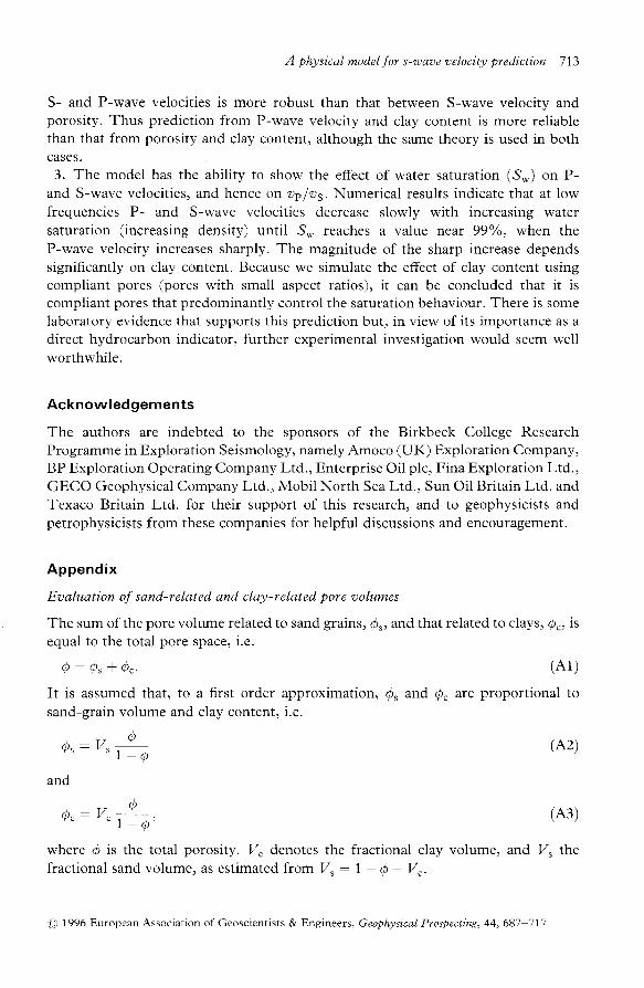
The sum of the pore volume related to sand grains, @., andequal to the total pore space. i.e.

Q - Q ' - t Q , '

that related to clays, @., is

( A l )

pc are proportional toIt is assumed that, to a first order approximation, /, andsand-grain volume and clay content, i.e.

66, : Vr;-: ,

L - Q

and

dQ c - V . l - , rr - ( p

(P'2)

(A3)

where @ is the total porosity. Z. denotes the fractional clay volume, andfractional sand volume, as estimated from V, : | - O - V..

O l996RuropeanAssociat ionof Geoscient is ts&Engineers, GeophysicalProspect ing,44,63T-717


T ime-aaerage and density equations

r , l : (1 - v r r [+v l r :and

r j : ( 1 - v : ) r : +v ' , r : .The density is found from

p- : (1 - V)pe- l V ' "p, .

In these equations f[ , f! and Zj are the P-wave transit times of the sand grains,

clay minerals and the mixture, fss, lns and Zj are the corresponding S-wave transittimes and pe, pc andp- the corresponding densities. Zi is the clay volume normalizedbv the volume of solid matrix:

. v ^L / ' -v c - _

I - Q

(A4)

Calculation of elastic moduli

The elastic bulk and shear moduli of the srain mixture are calculated from its transit

(As)

(A6)

(A7)

(A8)

(A1o)

( A 1 1 )

(A12)

(A13)

tlmes uslng

l r 4 \Km : P* \(rTf *;1q91

and

( | \Fm: Pm(r-=y/ (Ae)

Kuster and Toksciz (1974) give equations for evaluating the moduli of an elasticmedium permeated with a dilute ({ ( o) distribution of (non-interacting) ellipsoidalpores:

, K^ + 4Ap^l \ r : -" l - 3 4

and

l ta : l tm

where

1 + B ( 9 K - * 8 p - )1 - 6 8 ( K - + 2 p ^ ) '

A : ! K ' - K - \ - - , \n - t 3l<^ + 4u^ L a' t ;;ii\ar)'

B:+ffi 6,(r,,,11o,7_�ry),\-Z-/


A physical model for s-waae xelocitg prediction 715

Ka, K- and K' are the bulk moduli of the dry frame, the mixture and the fluid andlla, H^ and p,' are the corresponding shear moduli. K' and pr' are zero whencomputing the moduli of the dry frame (with empty pores). The scalars Ti;i1 andTi1;,1 are functions of the aspect ratio of the inclusions and the moduli and densities ofthe matrix and the fluid enclosed. The explicit expressions, given in Appendix B ofXu and White (1995a), correct a misprint in the equation for T;;;; in the originalKuster and Toksciz (1974) paper.

Gassmann equations

White (1965) formulated the Gassmann model for P-wave velocity zp as'": {" l"'-*"_,('-alc 2

c-(l - ot -r cro - 1!c dtf (A14)

(A17)

(A18 )

where pa : p^(l - il + pr d, Ka and p"6 are the bulk and shear moduli of the dryrock, and C^, Cr and C6 are, respectively, the grain matrix (matrix), fluid and dryrock frame compressibilities, given by

(A1s)

(A16)

t * : * ,

Ct: +;and

C . : *

The shear-wave velocity zs of the rock permeated by non-viscous fluid is simply

| \ l / 2

" ' - { & fl P n J

References

Blangy J.P. and Nur A. 1992. A new look at ultrasonic shear velocities in sands. SEG/EAEGsummer research workshop, Big Sky, Montana. Expanded Abstracts, 374-376.

Blangy J.P., Strandenes S., Moos D. and Nur A. 1993. Ultrasonic velocities in sands-revisited. G eophgsics 58, 344-356.

Bruner W.M. 1976. Comment on "Seismic Velocities in Dry and Saturated Cracked Solids"by Richard J. O'Connell and Bernard Budianskey. Journal of Geophysical Research 81,2573-2576.



Castagna J.P., Batzle M.L. and Eastwood R.L. 1985. Relationships between compressional-

wave and shear-wave velocities in clastic silicate rocks. Geophysics 50, 571-581.

Cheng C.H. and Toks<jz M.N. 1979. Inversion of seismic velocities for pore aspect ratio

spectrum of a rock. Journal of Geophysical Research 84,7533-7543.

Domenico S.N. 1976. Effect of brine-gas mixture on velocity in an unconsolidated reservoir.

G eophy sics 4I, 882-894.

Gassmann F. 1951. Elasticity of porous media. Vierteljahrschrift der Naturforschenden

Gesellschaft in Ztirich 96, l-21.

Gist G.A. 1994. Interpretation of laboratory velocity measurements in partially gas-saturated

rocks. Geophysics 59, 1100-1109.

Greenberg M.L. and Castagna I.P.1992. Shear-wave velocity estimation in porous rocks:

theoretical formulation, preliminary verification and applications. Geophysical Prospecting

40,195-209.Han D., Nur A. and Morgan D. 1986. Effect of porosity and clay content on wave velocity in

sandstones. Geophysics 51, 2093-2107.

Hornby B.E., SchwartzL.M. and Hudson I.A. 1994. Anisotropic effective-medium modelling

of elastic properties of shales. Geophysics 59, 1570-1583.

Hudson J.A. 1981. $7ave speed and attenuation of elastic waves in material containing cracks.

Geophysical Journal of the Royal Astronomical Society 64, 133-150.

Klimentos T. 1991. The effects of porosity-permeability-clay content on the velocity of

compressional waves. G e op hy sic s 5 6, l93O- 1939.

Klimentos T. and McCann C. 1990. Relationships between compressional wave attenuation,

porosity, clay content, and permeability of sandstones. Geophgsics 55, 998-1014.

Knight R. and Nolen-Hoeksema R. 1990. A laboratory study of the independence of

elastic wave velocities on pore scale fluid distribution. Geophysical Research Letters 17,

t529-r532.Kuster G.T. and Toksoz M.N. 1974. Velocity and attenuation of seismic waves in two phase

media: Part 1: Theoretical formulation. Geophysics 39, 587-606.

Marion D., Nur A., Yin H. and Han D. 1992. Compressional velocity and porosity in

sand-clay mixtures. Geophysics 57 , 554-563.Mavko G. and Jizba D. 1991. Estimating grain-scale fluid effects on velocity dispersion in

rocks. Geophysics 56, \940-1949.

Mukerji T. and Mavko G. 1994. Pore fluid effects on seismic velocity in anisotropic rocks.

Geophy sics 59, 233-244.

Murphy !7. 1984. Acoustic measures of partial gas saturations in tight sandstones. Journal of

Geophgsical Research 89, 1 1549-1 1559.

Rafavich F., Kendall C.H.St.C. and Todd T.P. 1984. The relationship between acousticproperties and the petrographic character of carbonate rccks. Geophysics 49, 1622-1636.

Rider M.H. 1991 . The Geological Interpretation of Well logs. Whittles Publishing, Caithness.

Serra, O. 1984. Fundamentals of Well-Log Interpretation. I: The Acquisitionof Logging Data.

Elsevier Science Publishing Co.Tosaya C.A. 1982. Acoustical properties of clay-bearing roc&s. Ph.D. thesis, Stanford

University.'Wang

Z. and Nur A. 1992. Elastic wave velocities in porous media: a theoretical recipe. In:

Seismic and Acoustic Velocities in Reservoir Rochs, Vol. 2, Theoretical and Model Studies (eds

Z.Vang and A. Nur), S.E.G., Tulsa, pp. 1-35.

O 1996 European Association of Geoscientists & Engineers, Geophysical Prospecting, 44' 687-717

A physical model for s-uaae aelocity prediction 717

\7hite J.E. 1965. Seismic Waz.ses: Radiation, Transmission, and Attenuatzbz. McGraw-HillBook Co.

\Tinkler K.r)f. and Nur A. 1982. Effects of pore fluids and frictional sliding on seismicattenuation. Geophysics 47, 1-12.

\food A.\7. 1941. A Textbook of Sound. The Macmillan Publishing Company, New York.Xu S. and \fhite R.E. 1995a. A new velocity model for clay-sand mixtures. Geophysical

Prospecting 43, 91-1 18.Xu S. and !(hite R.E. 1995b. Poro-eiasticity of clastic rocks: a unified model. 36th Annual

Logging Symposium, Paris, France, Transactions, Paper V.Xu S. and $7hite R.E. 1995c. Comparison of four schemes for modelling anisotropic P-wave

and S-wave velocities in sand-shale systems. 57th EAEG meeting, Glasgow, UK,Expanded Abstracts, Paper 82.

Yin H., Han D.H. and Nur A. 1988. Study of velocities and compaction on sand-claymixtures. Stanford Universitv. S.R.B. report 33.


Documents

XuWhite_1996 Shear Wave Velovity