X-811-74-62 - NASA...X-811-74-62 PREPRINT NASA TR1X4 70 #OVARIABLE-BEAMWIDTH MONOPULSE ANTENNAS R. F. SCHMIDT (!ASA-TM-X-706 5 0) VAIABLE-BEAW N74-25679 MONOPULSE ANTENNAS (NASA) CSCL

X-811-74-62PREPRINT

NASA TR1X4 70 #O

VARIABLE-BEAMWIDTH MONOPULSEANTENNAS

R. F. SCHMIDT

(!ASA-TM-X-70 6 5 0 ) VAIABLE-BEAW N74-25679

MONOPULSE ANTENNAS (NASA) CSCL 17BUnclas

G3/07 40597

MARCH 1974

PRICES SUBJECT TO CHANGE

S- GODDARD SPACE FLIGHT CENTERGREENBELT, MARYLAND

Reproduced by

NATIONAL TECHNICALINFORMATION SERVICE

US Department of CommerceSpringfield, VA. 22151

https://ntrs.nasa.gov/search.jsp?R=19740017566 2020-03-03T13:41:46+00:00Z

For information concerning availabilityof this document contact:

Technical Information Division, Code 250Goddard Space Flight CenterGreenbelt, Maryland 20771

(Telephone 301-982-4488)

X-811-74-62

Preprint

VARIABLE-BEAMWIDTH MONOPULSE ANTENNAS

R. F. Schmidt

March 1974

Goddard Space Flight CenterGreenbelt, Maryland


R. F. Schmidt

Network Engineering Division

ABSTRACT

This document discusses in detail the merits of nine methods for "zooming"

microwave amplitude-sensing monopulse antenna patterns. Of these, six are

directly related to the TDRSS (Tracking Data Relay Satellite System) and are

compatible with a deployable-mesh pseudo-paraboloidal main reflector. The

remaining three methods utilize radically different geometrical configurations

that depart considerably from the TDRSS parameters existing at this time.

Preservation of the monopulse postulates given by D. R. Rhodes is considered

to be of prime importance for any variable-beamwidth candidate, however, it is

allowed that approximate satisfaction of the postulates should be accepted for

practical reasons. All of the methods discussed herein admit free choice of the

polarization state, and the zooming function is never predicated on polarization.

The principles underlying five of the methods discussed are frequency independent.

Exploration of the zooming techniques was carried out almost entirely by

means of the Kirchhoff-Kottler vector diffraction program developed at Goddard

Space Flight Center. The program generates electric and magnetic field in-

tensity, associated phase, and time-average Poynting vector power flow in the

intermediate near-field and far-field zones in both receive and transmit modes

of operation. A few of the concepts have been verified experimentally with

excellent agreement between theory and practice.

Preceding page blank

oiii1

CONTENTS

Page

ABSTRACT ......... ................................ iii

ILLUSTRATIONS ...................................... vi

GLOSSARY OF NOTATION ............................... ix

INTRODUCTION ....................................... 1

CASSEGRAIN (DISPLACED HYPERBOLOIDAL ANNULUS) ............ 1

GREGORIAN (TRUNCATED ELLIPSOID) ...................... 7

CASSEGRAIN (NESTED PARABOLOIDS) ...................... 12

CASSEGRAIN (DEFOCUSSED HYPERBOLOID) .................. 13

CONICAL GREGORIAN (SPIRAL FEED) ....................... 16

TELESCOPING DUAL PARABOLIC CYLINDERS ................ 19

TELESCOPING PARABOLOID ............................. 21

CASSEGRAIN (DEFOCUSSED FEED) ................... ....... 23

GREGORIAN (DEFOCUSSED FEED) ......................... 24

CONCLUSIONS........................................ 24

ACKNOWLEDGMENTS .................................. 26

REFERENCES ......... .............................. 26

Preceding page blank

V

ILLUSTRATIONS

Figure Page

1 Cassegrain geometry with displaced hyperboloidal annulus .... 28

2 Tracking pattern, 2 -mode, ......................... 29

3 Tracking pattern, A -mode, .......................... 30

4 Acquisition pattern, 2 -mode,(truncated hyperboloidal annulus) ................. .... 31

5 Acquisition pattern, A-mode,(truncated hyperboloidal annulus) ..................... 32

6. Acquisition pattern, 2 -mode,

(8 = +4\ displaced hyperboloidal annulus) ................ 33

7 Acquisition pattern, A -mode,(8 = +4 X displaced hyperboloidal annulus) ............. ..... 34

8 Gregorian geometry with truncated ellipsoidal annulus ....... 35

9 Beamwidth versus subreflector diameter for modified

Gregorian system ................................ 36

10 Tracking pattern,l -mode, .......................... 37

11 Tracking pattern, A-mode, ........................... 38

12 Acquisition pattern,Y -mode, ........................ 39

13 Acquisition pattern,A -mode, ........................ 40

14 Nested Paraboloid Geometry ........................ 41

15 Acquisition patterns, 2 and A modes with main

paraboloid, ............................... 42

16 Acquisition patterns, I and A modes without main

paraboloid, .................................... 43

17 Tracking patterns, 2 and A modes with acquisition

paraboloid, ....... .... ..... ..... ................ 44

18 Tracking patterns, Z and A modes without acquisition

paraboloid, ...................................... 45

,19 Cassa n m V r.1y with defocussed hiype UoiiL . . . ............

20 Tracking patterns, Y and A modes (N = 77.3) .............. 47

vi

Figure Page

21 Acquisition patterns, 2 and A modes (N = 77.3)

for A Z = -3 /2 of hyperboloid ....................... 48

22 Acquisition patterns, Z and A modes (N = 77.3)

for A Z = -2 X of hyperboloid ......................... 49

23 Tracking patterns, 2 and A modes (N = 100) ......... ...... 50

24 Acquisition patterns, Z and A modes (N = 100)for AZ = -3X/2 ................................. 51

25 Acquisition patterns, Z and A modes (N = 100)

for AZ = -2 .................................... 52

26 Conical-Gregorian geometry with spiral antenna feed ........ 53

27 Primary radiation patterns of spiral antenna(a = 1/3, n = 1, 2, 3, 4) ............................ 54

28 Tracking patterns, 2 and A modes, of the Conical Gregorian

System (a = 1/3, n = 1, 2) ........................... 55

29 Acquisition pattern, A mode, of the Conical Gregorian System

(a = 1/3, n = 4).................................. 56

30 Dual parabolic cylinder geometry ..................... 57

31 Acquisition pattern, Channel I (2) ..................... 58

32 Acquisition pattern, Channel I (A) ..................... 59

33 Acquisition pattern, Channel II (2). ............. ......... 60

34 Acquisition pattern, Channel II (A) ...................... 61

35 Tracking pattern, Channel I (Z) ....................... 62

36 Tracking pattern, Channel I (A)......................... 63

37 Tracking pattern, Channel II (2) ...................... 64

38 Tracking pattern, Channel II (A) ...................... 65

39 Electric-field distribution (ACQ) .................. ...... 66

40 Wavefronts (ACQ) ............................... 67

41 Time-average Poynting vectors (ACQ) ................. 68

42 Electric-field distribution (TRK) ...................... 69

43 Wavefronts (TRK).....* ........................... 70

vii

Figure Page

44 Time-average Poynting vectors (TRK) .................. 71

45 Telescoping-paraboloid geometry ...................... 72

46 Electric-field distribution (ACQ) .................. .... 73

47 Wavefronts (ACQ) ............................... 74

48 Time-average Poynting vectors (ACQ) .................. 75

49 Acquisition pattern, Channel I (2) ( = 0', 180' ) ........... 76

50 Acquisition pattern, Channel I (A) (¢= 00, 1800 ) ........... 77

51 Acquisition pattern, Channel I (2) (¢= 900 ) ............... 78

52 Acquisition pattern, Channel I (A:) (t= 900 ) ............... 79

53 Acquisition pattern, Channel II (2) (P = 900) .............. 80

54 Acquisition pattern, Channel II (@) (p = 900). ................. 81

55 Acquisition pattern, Channel II (2) (,= 00, 1800) ........... 82

56 Acquisition pattern (Y) of defocussed Cassegrain .......... 83

57 Acquisition pattern (A) of defocussed Cassegrain .......... 84

58 Acquisition pattern (2) of defocussed Gregorian .......... 85

59 Acquisition pattern (A) of defocussed Gregorian .......... 86

viii

GLOSSARY OF NOTATION

Symbol Meaning

F, F* focus, conjugate focus

a radial extent of reflectormax. aoo

X wavelength

f frequency

A, C, a, c hyperboloid and ellipsoid constants

LI integration sampling interval in wavelengths

P(I), P(J), P(K) components of polarization moment

Te feed displacement vector (x , YE z )

N i feed directivity factor in E i = S. cosNi 9

Si feed strength or weight factor

qPi initial phase of source

CPU time central processor unit time

GHz giga-Hertz

2, A sum and delta monopulse modes

Yi reflecting surface

a, 3, y Euler angles

<P> time-average Poynting vector

r, 0, radial and angle variables of spherical coordinate system

ACQ acquisition mode

TRK tracking mode, or data mode

ix

BW beamwidth

9, <D angle-variables for feed system

3, A a perturbation or difference

R, r radius or range

D, d diameter

M magnification factor

E eccentricity

GD(8 , ( ) directive gain

E, H electric and magnetic field vectors

A area

a spiral growth-rate parameter

n spiral mode parameter

/3, k wave number designations

F (0) spiral-pattern amplitude function

P (0) spiral-pattern phase function

In natural logarithm

x


INTRODUCTION

Antennas with highly directive gain (BW < 10, say) are well-suited for high-

precision monopulse angle-tracking, but have an inherent acquisition problem.

There would be a distinct advantage to annexing a step-wise or continuously

variable "zoom" capability, particularly if that capability could be achieved with

the original antenna structure. Frequency is an obvious degree of freedom. For

these cases where frequ'ency cannot be changed it is necessary to look for other

means, such as the reduction of the effective diameter of the main reflector

aperture of the system, to increase the beamwidth of the radiation patterns.

Optical "zoom" systems traditionally effect a change of focal-length to vary the

field of view. Iris techniques, defocussing, and a host of other approaches have

also been proposed. The present discussion is restricted to methods which (1)satisfy the monopulse postulates, 1 at least in a practical context, and (2) allow

freedom of choice with regard to the system polarization state, usually circular,

and specifically do not utilize polarization techniques to achieve zooming. It is

implicit that an increase in beamwidth results in a reduction in directivity gain

and therefore system gain. The subsequent development will show that, ingeneral, the system gain will be reduced even further due to spillover losses,defocussing losses, circuit element losses, and other miscellaneous losses as-

sociated with zooming. Violation of the monopulse postulates will impose addi-

tional penalties at the receiver and this in turn will affect overall system

performance.

This interim report is intended to illustrate some basic approaches for

achieving variable beamwidth Ku-band monopulse antenna designs, but makes

no attempt to optimize any of these with regard to sidelobe levels, gain, etc.The following table is provided to identify the nine geometrical configurations

treated in detail, together with some of their general characteristics pertinentto the TDRSS.

CASSEGRAIN (DISPLACED HYPERBOLIC ANNULUS)

Figure 1 shows the geometry used to probe the possibilities of zooming a

Cassegrain system by displacement of a hyperboloidal annulus away from a

hyperboloidal cap. The objective, initially, was to obtain approximately 50%

increase of beamwidth. Ideally, one would prefer to truncate the hyperboloid

1Ref. 1, pages 21-23 (a) angle sensing has a group inverse, (b) angle information forms as a ratio(c) the angle output function is an odd real function of the angle of wave arrival.

1

Geometry Type of Zooming Beamwidth Mode of Ku/S-BandIncreaset Operation Dichroic Subreflector

1. Cassegrain* discrete-step 50 to 75% electro- requiredwith Displaced Hyper- mechanicalbolic Annulus

2. Gregorian with Trun- fixed ratio 100% with electro- not requiredcated Ellipsoid S-band mechanical

200% withoutS-band

3. Cassegrain with** fixed ratio 400 to 600% electrical requiredNested. Paraboloids

4. Defocussed Cassegrain* continuously 100 to 300% electro- requiredwith Di splaced Hyper- variable mechanicalboloid

5. Conical Gregorian discrete-step 150% electrical not requiredwith Spiral Feed (error channel)

6. Dual Parabolic bi-directional nominally electro- not requiredCylinder continuously 100% mechanical

variable

7. Telescoping continuously nominally electro- not requiredParaboloid variable 100% mechanical

8. Defocussed Cassegrain* fixed ratio 100 to 200% electrical requiredwith Displaced Feed

9. Defocuessed Gregorian* fixed ratio 100 to 200% electrical not requiredwith Displaced Feed

*Frequency dependent**This approach could also be used to satisfy a scan requirement since it is possible to gimbal the nested paraboloid.t Upper and lower bounds have not been established for the different methods.

of an unaltered Cassegrain, but it is necessary to physically dispose of thetruncated portion. In fact, the vector diffraction simulation 1 used in thesestudies developed a truncated approach at the outset since the displaced hyper-boloidal annulus problem required a composite surface capability which was notavailable. The hyperboloid is regarded as a disjoint composite surface for theacquisition case, and a contiguous composite surface for the tracking case, by

2the program in a special subroutine.

The hyperboloidal annulus was deliberately driven away from the paraboloidso that it would enter an umbral region. If, conversely, the hyperboloidal annuluswere driven toward the paraboloid, an interference situation would be set upwhereby portions of the annulus would tend toward phase stationarity in theaperture plane while other portions of the annulus would tend toward non-stationaryresults. Furthermore, this situation would change drastically as the annuluswas displaced along the system (Z) axis. The question of "optimum" displace-ment was studied in detail with the following conclusion.

Twenty different displacements of the hyperboloidal annulus (0 X < 8 < 10K)indicated that the amount of zooming was considerably less than the desired 50%increase for 0 < 8 K, considerably greater than 50% and highly erratic for

< 8 _ 3.75K , and between 40% and 70% for 3.75 X 8 <10K. In the latterregion, the behavior was still oscillatory (±10%), but not violently so. It wasalso noted that the resulting radiation pattern sidelobe levels were poor in theregion K < 8 < 3X, but were about -20 db in the region 3 x < 8 10 withN = 8 in the source pattern E = S cosN 9, corresponding to -10 db. edge-taperon the original hyperboloid. The displacement 8 = +4X was chosen for subsequentstudies since it was the minimum physical displacement consistent with reason-able performance (43% zooming) using a pencil beam only at this stage of thedevelopment.

Approximately 200 radiation patterns were then computed using vectorKirchhoff-Kottler diffraction theory to develop this approach to zooming themonopulse patterns. The findings are summarized as follows.

Subsystem patterns at a distance R = F were computed for the normal sys-tem (unmodified hyperboloid), a truncated hyperboloid, and a displaced hyper-boloidal annulus (3 = +4K). The normal system showed an edge taper of about-10 db, due to subsystem backscattered pattern directivity alone, directed towardthe edge of the paraboloidal main reflector. The associated phase characteristicwas that of a typical virtual point source at F ( = constant ±10 electrical degrees).

1Ref. 22 Hyperboloid truncation is predicated on BW = 70 V/De for the paraboloid without regard to

illumination distribution initially. BW is selected, De is determined, and ray-optics providesthe intercept on the hyperboloid.

3

Not surprisingly, the idealized truncated subsystem showed an edge taper ofabout -25 db at the paraboloid due to the backscattered pattern, but the wavefront was not characteristic of a spherical wave over the region of interest,1160 < E < 1800. A nearly phase linear gradient ranging over about 300 elec-trical degrees was observed in the region 1160 a 1450 with an oscillation of±20 electrical degrees over the region 1450 < E 1800. Finally, the displacedhyperboloidal annulus case showed only -15 db edge taper at the paraboloid with±5 db oscillations over the entire range of interest. A nearly linear phasegradient ranging over about 500 electrical degrees was observed in the region1160 0e 1450 with an oscillation of ±30 electrical degrees over the region1450 < 0 1800. These diffraction results give considerable insight concerningthe mechanics of zooming, and indicate a stronger dependence on phase station-arity than might be determined from ray-tracing alone.

An analysis of the Airy disc and bright-ring structure was carried out forthis Cassegrain configuration. The magnification factor of the system is

E+1M-

E-1

where

= [1 + (a/c) 2]1/2,

for the original set of parameters (i.e. before truncation or displacement of thehyperboloidal annulus). From a ray-tracing argument alone, under-illuminationof a paraboloidal annulus should result in a smaller effective main aperturediameter and, therefore, a larger Airy disc diameter. In the event that theacquisition mode is actually attained by phase incoherence (non-stationarycontributions) at the edge of the paraboloid, the conclusion is the same.

The size of the focal bright-spot or Airy disc for a paraboloid is given by

R = 1.22 Fk/D = 0.488k

for a. V. 5-foot diameter refiecLor with 5.0-foot focal length. Since the magni-fication factor (M) for the system is approximately equal to 2.6, by the formulaabove or graphically by the equivalent-parabola approach for dual-reflectorsystems, the Airy disc radius should be about

4

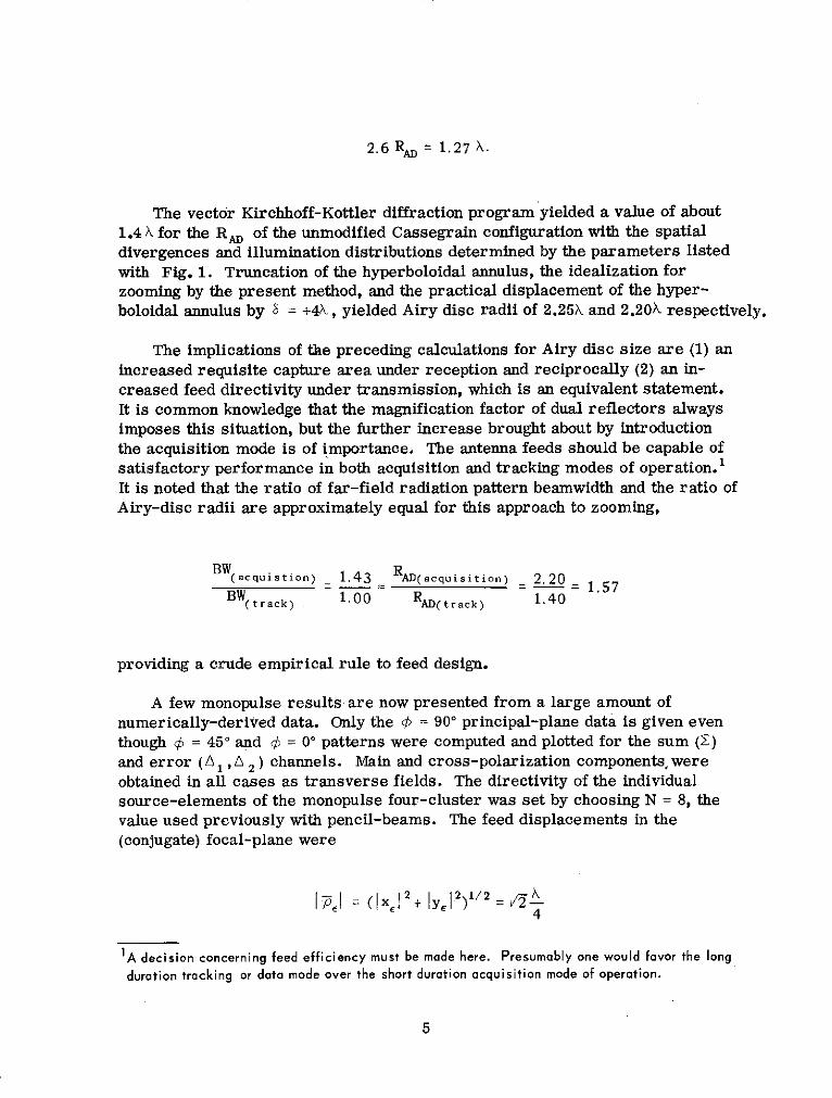
2.6 RA = 1.27 X.

The vector Kirchhoff-Kottler diffraction program yielded a value of about1.4 k for the RAD of the unmodified Cassegrain configuration with the spatialdivergences and illumination distributions determined by the parameters listedwith Fig. 1. Truncation of the hyperboloidal annulus, the idealization forzooming by the present method, and the practical displacement of the hyper-boloidal annulus by 8 = +4k, yielded Airy disc radii of 2.25k and 2.20k respectively.

The implications of the preceding calculations for Airy disc size are (1) anincreased requisite capture area under reception and reciprocally (2) an in-creased feed directivity under transmission, which is an equivalent statement.It is common knowledge that the magnification factor of dual reflectors alwaysimposes this situation, but the further increase brought about by introductionthe acquisition mode is of importance. The antenna feeds should be capable ofsatisfactory performance in both acquisition and tracking modes of operation.'It is noted that the ratio of far-field radiation pattern beamwidth and the ratio ofAiry-disc radii are approximately equal for this approach to zooming,

BW(acquistion) _ 1.43 RAD(acquisition) 2.20 1.571.57

BW(track) 1.00 RAD(track) 1.40

providing a crude empirical rule to feed design.

A few monopulse results are now presented from a large amount ofnumerically-derived data. Only the € = 900 principal-plane data is given eventhough ¢ = 450 and ¢ = 0' patterns were computed and plotted for the sum (2)and error (, A 2 ) channels. Main and cross-polarization components, wereobtained in all cases as transverse fields. The directivity of the individualsource-elements of the monopulse four-cluster was set by choosing N = 8, thevalue used previously with pencil-beams. The feed displacements in the(conjugate) focal-plane were

I= (Ixj2+ YI 2)'1/2 = 24

IA decision concerning feed efficiency must be made here. Presumably one would favor the long

duration tracking or data mode over the short duration acquisition mode of operation.

5

where I x = I y I also. On the basis of the system magnification factor, thisis not an optimum choice. Nevertheless, the zooming effect can be displayedvery effectively. Monopulse feed clusters with 12 and 16 sources, variouslydisplaced, and with different directivity (N) were used in the simulation, how-ever, this work was not completed because of the numerous combinations thatneed to be explored.

Figure 2 gives the k = 900 cut on the 2 channel (main-pol. component). At-tention is directed to the constant phase of the monopulse reference channel ofthe angular domain 0 < 0 < 0.40, which is well beyond the maximum trackingangle. Now this is the reference pattern for the track mode of operation. Thecorresponding error channel, A1, is given by Fig. 3, and again, attention isdirected to the phase of that channel over the angular domain 0 < 6 < 0.40. It canbe seen that the simulation verifies, with excellent numerical fidelity, the mono-pulse postulates for this amplitude-sensing system, showing a phase jump of180 electrical degrees upon traversing the boresight axis.

Figure 4 gives the 0 = 900 cut on the : channel for the acquisition mode ofoperation for idealized truncation of the hyperboloidal subreflector, and Fig. 5gives the corresponding A channel. Once again, it can be seen that a "clean"discontinuous 180 electrical degree phase jump exists at boresight. It shouldalso be noted that phase is constant over the domain 00 < 0 < 0.40 which is thelimit of tracking based upon the error channel maximum for this (idealized)set of acquisition patterns.

Figure 6 gives the € = 900 cut on the Y channel for the acquisition mode ofoperation for the more practical case with a displaced hyperboloidal annulus,and Fig. 7 gives the corresponding A channel. For this situation the same "clean"discontinuous 180 electrical degree phase is observed, however, the phase of the2 and A channels is now constant over the angular domain 00 6 0.40 to within±5 electrical degrees or so, which is a negligible perturbation on the trackingreceiver. It is not definite, at this writing, whether the ±5 degree phase varia-tion is artificially induced by the integration sampling interval on the main- andsub-reflector (LI,= LI 2 = 0.5 wavelengths), or an actual property of the zoomedantenna. In any event, the effect is a minor one. Further work can always bedone to verify the stability of the numerical evaluation by selecting successivelysmaller LI intervals.

The subject of system gain is an important consideration in the selection ofa beam-zooming technique. Zooming inherently implies a reduction in directivityand, therefore, system gain. In the present case, however, there is an additionalloss due to spillover at the edge of the hyperboloidal cap for large physical dis-placements of the hyperboloidal annulus away from the paraboloid, and somedefocussing loss for very small physical displacements of the annulus. For the

1All phases are modulo 360 electrical degrees.

6

set of monopulse patterns discussed in this document, first indications based onthe computed monopulse sum (:) pattern levels indicate a loss of 8.1 db and0.6 db for the truncated and displaoed annulus oases, respectively. This can becontrasted wit -a .1b loss p rdied on a 43% beamwidth increase. Theimplication is that approximately 8,0 db and 2.4 db of loss is incurred by spill-over and defocussing offects for the preceding idealized and practical casesrespectively, It is not known whether the computed raw levels of the patternsare a reliable measure for relative (or absolute) gain determination in all casesunder superposition. It is known that an integration of the secondary pattern incomplete generality, leads to the correct gain figures providing the integrationis carefully executed and the computed pattern is valid for large angles awayfrom boresight. The latter integration capability is now being annexed to theprograms being used for zoom calculations.

In conclusion, this first method for zooming is mechanical in nature, canachieve discrete steps of zooming by utilization of several annular hyperboloidalsections, can provide about 50% of beamwidth increase, has poor spillovercharacteristics (~ so), and requires a dichroic hyperboloid if S-band is to co-exist with Ku-band on the TDRSS. 1

GREGORIAN (TRUNCATED ELLIPSOID)

Figure 8 shows the geometry used to probe the possibilities of zooming aGregorian system by trunostion of an ellipsoidal subreflector, The objectives,dictated primarily by TDRSS requirements, were extended to include 100% to200% inz'ease of beamiwidth, electrical instead of mecha ial means of operationi,Ku-band zooming compatible with S-band tracking functions, and rapid switchingbetween wide-angle (acquisition) and narrow-angle (tracking) modes. It has al-ready been stated that free choice of polarization state, usually circular, wasprerequisite, together with satisfaction of the monopulse postulates. Continuedstudy of the zoom problem has resulted in more stringent objectives. Ideallythe sum and difference patterns should zoom without null filling, the n -radiandiscontinuous phase jumps should be preserved, sidelobe characteristics shouldnot be overly degraded, error-channel slope should exhibit monotonic char-acteristics, an approach to "fail-safe" design should be evolved, antenna tem-perature characteristics should conform to the mode of operation, and elimina-tion of the dichroic element (for achieving S-band capability together withKu-band zoom capability) should be considered. Finally, means should be soughtto eliminate, or at least minimize, spillover loss associated with the zoomingprocess so that system or link gain is reduced by the directivity gain factoralone if possible.

1Ref. 3

7

The logic for achieving zooming by truncation of the ellipsoidal member ofa standard Gregorian configuration is elementary.1 Ray-tracing through confocalsystems results in 1:1 mappings, or isomorphisms, excepting the final m:1 map-ping to the -conjugate focus (F*). Under-illumination of an annulus of the main(paraboloid) reflector of a Gregorian arrangement will result in zooming. Trac-ing rays through the system in the receive-mode of operation truncates the sub-reflector in accordance with the desired amount of zooming or effective diameterpostulated for the paraboloid. In this way, the focus F* becomes available forthe acquisition mode, and the focus F becomes available for the track mode ofoperation. Compatibility with the S-band function sets constraints on the rangeof parameters that can be employed for the ellipsoid since an S-band trackingfeed, also at focus F and nested with the Ku-band tracking feed, obscures asignificant portion of the ellipsoid. The ellipsoid cannot be increased arbitrarilyto relieve the situation, however, since it in turn obscures a significant portionof the paraboloid. Figure 8 represents a particular compromise in which about3 percent of the ellipsoid and 5 percent of the paraboloid are obscured (blocked)before truncation. Obviously, with such an arrangement, wide-beam designs willreduce obscuration of the paraboloid while increasing obscuration of the ellip-soid. It is noted that some degradation of the acquisition-mode beams wouldprobably be tolerable since the percentage of time allocated to acquisition ispresumably much less than that allocated to data collection in the track-modeof operation.

The modified Gregorian configuration of Fig. 8 satisfies the objectives,discussed above, to a very high degree. It can be seen that redundant electricalswitching can be provided for rapid change-over between acquisition and trackingfunctions. No polarization constraints are introduced to achieve zooming. Ray-optics alone essentially guarantees satisfaction of the monopulse postulates,however, this was verified by Vector Kirchhoff-Kottler diffraction analysis andis discussed later inthis report. It is also noted that the antenna noise tempera-ture for the data or tracking mode will tend to be lower than for the acquisitionmode since spillover from F is more apt to be directed at the cold sky, whereasspillover from F* around the subreflector is more apt to "see" the hot earth.There are, then, at least two reasons for having a high edge-taper for the acquisi-tionfeed: (1) antenna noise temperature reduction, and (2) minimization of gain lossdue to truncation of the ellipsoid to achieve zooming. A dichroic subreflectoris not required, even with S-band tracking functions on board since, for a Gregorianconfiguration, the feed points or foci are between the reflecting elements. It isnecessary that the tracking feed arrangement be such as to permit energy toimpinge on the ellipsoid during the acquisition phase. Retracting that feed is anobvious mechanical approach, but presents practical difficulties. Utilization of

1 Ref. 4

8

feed point F also has the disadvantage of placing electronics at a large distance

from the main reflector. Radiation pattern characteristics for the Ku-band

zoom mode of operation as determined by the analytical/numerical Kirchoff-

Kottler simulation, are now discussed in detail.

Subsystem patterns at a distance R = F were computed for the normal system

(unmodified ellipsoid, cmax. = 1.4') and for a range of radii representing different-

size ellipsoids and, therefore', different zooming ratios. The following discussion

summarizes some of the findings. Reduction of the size of the ellipsoid resulted

in progressively larger edge-taper on the main or paraboloidal reflector. An

isotropic amplitude pattern (E = S cosN 9, N = 0) was used as a prime feed func-

tion, even though this is a pessimistic approach in terms of spillover ('Tsol) at

the subreflector. It was noted that the wave backscattered from the ellipsoid

was a classical virtual spherical wave with regard to both amplitude and phase

at the outset for zero increase of beamwidth. As progressively smaller ellip-

soidal subreflectors were introduced, the geometrical bound over which a

spherical wavefront could be observed became more restricted. In the vicinity

of the paraboloid limbs, the phase was no longer a constant, as for the spherical

wave, but exhibited a nearly linear gradient ranging over some 1600 electrical

degrees for the extreme case (truncated ellipsoid, o- x.= 0.4'). The phase

oscillations in the angular domain were also increased as higher zoom ratios

were approached. The phase of the spherical wave associated with the unmodi-

fied system was constant to within ±20 electrical degrees over the angulardomain 1160 a < 1800. These oscillations increased to ±40 electrical degrees

for the extreme case of zooming cited above. The mechanics of zooming by the

present method were identified as a simultaneous reduction of backscattered

field strength, as predicted by ray-optics, and the introduction of phase inco-

herence with respect to the aperture-plane of the paraboloid. Both effects

therefore tended to make an annulus of the paraboloid ineffective (an umbral

region), thereby reducing the effective diameter of the main reflector and in-

ducing the increase of beamwidth, or zooming, desired.

The Airy disc and bright-ring structure in the vicinity of the conjugate

focus was not mapped, for Gregorian configuration, using the intermediate near-

field capability of the program. It has been shown previously, for the Cassegrain

configuration, that the effects are somewhat predictable once the magnification

factor of the dual reflector system has been computed. For the Gregorian, the

magnification factor is

E+1M-E- 1

where

[l - (a/c)2 ] 1/2

9

for the original set of parameters (i.e. before truncation of an ellipsoidal annulus.)There may be some merit to plotting the Airy diffraction structure for thezoomed case, particularly where a system is to be built and certain character-istics are to be optimized. This report was concerned with the feasibility ofzooming, and first-principles only. It therefore utilized abstractions such asN - 0 for the prime-feed functions, etc. In addition, it was thought that it wasmore profitable to search for other approaches to the TDRSS zooming problemthan to dwell on the optimization of any one method at this time.

The zoom phenomena for the modified Gregorian configuration was observedinitially for pencil-beams (one source, i 1). Uncontrolled spillover loss (s o)exists here. Approximately 200% beamwidth increase appears attainable, how-ever, only 100% beamwidth increase appears likely if simultaneous Ku-band andS-band operation is a condition. This situation, incidentally, leads to approxi-mately 4% of obsouration of the paraboloid by the truncated ellipsoid, and 4% ofobsouration of the truncated ellipsoid by the S-band feed. Figure 9 is a compositeplot illustrating beam width for various ellipsoidal subreflectors. The beamlevels are those resulting from the Kirchhoff integration, a linear superpositionprocess. No attempt was made here to verify the integration levels with thedefinition of directive gain, although this feature is being annexed to the programsused for zoom-technique investigation,

In the future, an adequate number of azimuthal far-field radiation patterncuts will be taken on each pattern so that the integral

CbG(9, )= E2 (Q, )

7-JJ E2(0, O) sin 6d~d¢

can be evaluated meaningfully to determine directive gain. For the present, theraw integration levels are available as an estimate of relative field strength forvarious conditions of zooming. The implication is that the signal level changesof Fig. 9 are a measure of directivity gain loss and spillover loss at theellipsoidal subreflector for an isotropic source at the conjugate focus (F*).

Monopulse patterns, under ideal conditions, exhibit discontinuous 7n -radianphase jumps at their radiation pattern amplitude nulls in the angular (0) domain.At least this is true for those systems which have biplanar symmetry (four feedsor four groups of feeds). Certain exceptions exist. For the case at hand, com-monly referred to as three-channel monopulse (2, A1, A2 ), the relative phase

10

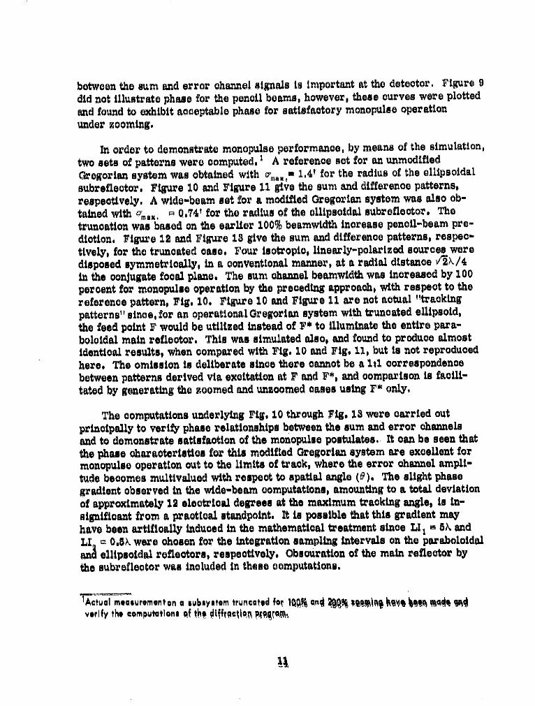
between the sum and error channel signals is important at the detector. Figure 9

did not illustrate phase for the pencil beams, however, these curves were plottedand found to exhibit acceptable phase for satisfactory monopulse operationunder zooming.

In order to demonstrate monopulse performance, by means of the simulation,two sets of patterns were computed. 1 A reference set for an unmodified

Gregorian system was obtained with m,,om 1.4' for the radius of the ellipsoidal

subreflector. Figure 10 and Figure 11 give the sum and difference patterns,respectively. A wide-beam set for a modified Gregorian system was also ob-

tained with c~,x, ; 0.74' for the radius of the ellipsoidal subreflector. Thetruncation was based on the earlier 100% beamwidth increase pencil-beam pre-diction. Figure 12 and Figure 13 give the sum and difference patterns, respec-tively, for the truncated case, Four isotropi, linearly-polarized sources weredisposed symmetrically, in a conventional manner, at a radial distance 4~\/4in the conjugate focal plane. The sum channel beamwidth was increased by 100percent for monopulse operation by the preceding approach, with respect to the

reference pattern, Fig. 10. Figure 10 and Figure 11 are not actual "trackingpatterns" since, for an operational Gregorian system with truncated ellipsoid,the feed point F would be utilized instead of F* to illuminate the entire para-boloidal main reflector. This was simulated also, and found to produce almostidentical results, when compared with Fig. 10 and Fig. 11, but is not reproducedhere. The omission is deliberate since there cannot be a 1:1 correspondencebetween patterns derived via excitation at F and F*, and comparison is facili-tated by generating the zoomed and unzoomed oases using F* only,

The computations underlying Fig. 10 through Fig. 13 were carried outprincipally to verify phase relationships between the sum and error channelsand to demonstrate satisfaction of the monopulse postulates. It can be seen thatthe phase characteristics for this modified Gregorian system are excellent formonopulso operation out to the limits of track, where the error channel ampli-tude becomes multivalued with respect to spatial angle (0). The slight phasegradient observed in the wide-beam computations, amounting to a total deviation

of approximately 12 electrical degrees at the maximum tracking angle, is in-significant from a practical standpoint. It is possible that this gradient mayhave been artifically induced in the mathematical treatment since LI1 - A andLI - 0.5h were chosen for the integration sampling intervals on the paraboloidalan ellipsoidal reflectors, respectively. Obsouration of the main reflector bythe subrefleotor was included in these computations.

ActuaI measurementon a subsystem truncated foe 1o!4V and h /S k t" Be asverify the computations of the tOtfrptosi p;agJsmq

41

In conclusion, good noise temperature characteristics, control of spilloverlosses, deletion of a dichroic subreflector and approximately 100% beamwidthincrease are attainable with this system, but mechanical difficulties associatedwith retracting the feed and placing electronics at focal point F are disadvantages.

CASSEGRAIN (NESTED PARABOLOIDS)

Figure 14 is a typical "nested paraboloid" arrangement which could con-ceivably be adapted to utilization on the TDRSS. The geometry was contrivedso that the main paraboloid suffers a 6.4 percent obscuration by the smallerparaboloid which, in turn, is obscured in the same degree by the hyperboloidal(dichroic) subreflector. Although the support cone was originally a continuousmetallic surface, it is probably feasible to employ structural members only atits base so that the radiation pattern of the acquisition feed can view the smallerparaboloid. The F/D ratio was made equal for both the acquisition and trackparaboloids, but need not necessarily be set in this way. The arrangementshown in Fig. 14 could probably be achieved for the dual-mesh TDRSS reflectorby adjusting the ties between the meshes. In the present application, the TDRSSlink will not allow much more than 200 percent of beamwidth increase. Obscura-tion of the acquisition paraboloid by the hyperboloidal (dichroic) subreflector be-comes increasingly important as the acquisition antenna size is reduced.

The following figures show the acquisition and tracking patterns of thenested system. In all cases, obscurations are taken into account. For theacquisition case, the hyperboloid of the Cassegrain arrangement consititutes anobscuration of the small acquisition paraboloid. The spillover of the acquisitionfeed is incident on the main or tracking paraboloid, and this effect is also takeninto account. See Fig. 15. If there were only the obscuration due to the hyper-boloid, the acquisition patterns would appear as in Fig. 16. These two figuresare not greatly different, which is to be expected since the law of curvature ofthe main parabola (as seen from the focal point of the acquisition feed) will leadto phase incoherent contributions. In addition, these individual contributions,resolved to an LI of 2.0 (wavelengths), are weak since an edge taper of -10 dbwas employed for the acquisition paraboloid.

When the tracking pattern is formed, the small acquisition paraboloid actsas a boss or "deformation" of the main paraboloid. A composite surface sub-routine was used here to accommodate the two parabolic laws of curvature whenthe antenna was used as a Cassegrain configuration. The "deformation" is, ofcourse, partially obscured by the hyperboloid. Figure 17 shows the results forTDRSS parameters. If the small acquisition paraboloid were not present, andonly the obscuration due to the hyperboloid were taken into account, the resultswould be as shown in Fig. 18. A few rather small effects, then, are attributable

12

to the disturbing influence of the acquisition antenna. Figure 17 reveals a

reduction in axial gain of about 1.3 db, and a slight narrowing of the beam. The

latter can be accounted for since the adverse law of curvature introduced by the

acquisition antenna is effectively only a large obscuration of the central region

of the main or tracking paraboloid, which leads to weak interferometric effects

(i.e. beam narrowing and a 7 db increase in sidelobe levels).

In conclusion, the nested paraboloid approach is straightforward and provides

a significant beamwidth increase with no gain degradation due to surface-

truncation. The penalty for nesting paraboloids is a mutual degradation of the

acquisition and tracking or data collection functions.

CASSEGRAIN (DEFOCUSSED HYPERBOLOID)

Figure 19 shows the geometry used to investigate monopulse zooming with

the parameters of the TDRSS main reflector. The hyperboloid was displaced

toward the main reflector according to a known principle, 1 which avoids in-

creased spillover loss when zooming to wide beam operation. A continuously

variable zoom ratio would appear to be obtainable via mechanical displacement

of the subreflector. It was found, for the parameters used in the present simu-

lation at least, that the zooming action is sluggish with respect to the amount of

hyperboloid displacement used until one wavelength of displacement has been

reached. Thereafter several hundred percent of zoom can easily be attained,

but the phase relationships between the monopulse sum and difference patterns

must be verified to obtain an optimum working system. In the event that the

phase of the sum (Z) channel is arbitrarily distinct from the phase of the differ-

ence (z1) channel at boresight, compensation can be made. A fixed length of

line at the antenna, or a phase adjustment at the monopulse receiver, will correct

the situation. In the event that the phase variation with angle (6) from boresight

for the channels is given by functions qi(8) and A 1 (8), then

kb2(e) - A (")! = A4(O)

must be no greater than about 30 electrical degrees since there appears to be

no simple means of removing a theta-dependent phase variation.

Investigation of this defocussed Cassegrain configuration tended to show

that the zooming capability was highly dependent on the directivity associated

with the monopulse source elements, somewhat dependent on the source separa-

tion, and independent of the amount of hyperboloid displacement if the preceding

parameters were not conducive to zooming. For example, for radial feed dis-

placements of /_V/4 in the conjugate focal plane, a directivity obtained via

'Ref. 5, Ref. 6

13

N = 50 in the feeood function E S osN 0 failed to produce beam widening of thequality desired even for displacements Z - - 10a . for the hyperboloid, A valueof N 100 produced good to excellent results for hyperboloid displacements assmall as a Z -a 8 3 /2 and A Z - 2 h,

A separate detailed study of the subsystem with displaced hyperbola yieldedsome insight concerning the mechanics of zooming by the method under discus-sion, This study was actually motivated to improve the methods of gain calcu-lation, which entailed computing the energy incident on the paraboloid when thehyperboloid is displaced, The reasoning was that the energy could be countedeasily within the framework of the existing program by displacing the entiredefocussed Cassagrain system providing a virtual spherical wave could be iden-tified for the defocussed subsystem, It was found that such a displaced virtualspherical wave did in fact exist, for all practical purposes, and that it appearedto emanate at a point in space that was displaced toward the paraboloid. Theamount of the displacement was approximately equal to the hyperboloiddisplacement for those cases studied. Displaeoment of the hyperboloid In theCassograin system is, therefore, equivalent to an axial displacement of adirective point source in a front-fed paraboloid. It was noted that the edge-taperat the hyporboloid limb was sensibly unaffocted in achieving zooming by thismethod, which is indicative of the fact that phase incoherence underlies thiszooming technique, This may be contrasted with the previously discussedGregorian system which was modified by truncation of the ellipsoidal sub-reflector. In that approach to zooming, subsystem pattern amplitude playedthe dominant role,

Two sets of far-field monopulso patterns are now presented, depicting thesituation when N = 77.8 and N - 100, for radial feed displacements of /-A/4 inthe focal plane. These correspond to feed tapers of -17 db and -20 db, respec-tively, at the hyperboloid edge before displacement of that subrefleotor. Fiure20 Is the reference pattern with N m 77.3 and shows the sum and diffeorncepattern amplitudes and phases, Figure 21 and Figure 22 show the same patternswhen the hyperboloid has been displaced toward the main reflector by an amountA Z / - 3/2 X and -2V. It is noted that for the lower value of edge-taper (-17 db)at the hyperboloid edge, the amplitude of the difference pattorn exhibits a regionwhere the slope is monotonically Increasing but close to zero (0.25 4 il 4 0.401)when A Z 3 -/2 . This is not desirable, The relative phase between sum anddifference channels in Figure 21 is accoptable for acquisition. Increoaing thehyp rJloId displacement to -2 , Fig. 22, results in a poor relative phase

at imnk hin af tnnn Ot sum and difference chAf nneh , oone whIch I4 not easilye89p~W}Pa3 e ani tfhe poet of Nifurcation can be observed in the sum channel.A 7Folo 9r Pr-PlP wP P fll sloe (pe (,~o r 0.250) is still in evi-dni4es W hm 8.s At §9MRw00 0lPtOi t0 Ne p ropedinR xq ple

14

The second set of patterns, obtained with increased edge-taper (-20 db) atthe hyperboloid edge showed better monopulse characteristics. Figure 23represents the reference pattern. Figure 24 and Figure 25 correspond to dis-placements of AZ -: - 3/2 X and A Z = - 2 . The first of these is excellent foracquisition. There is no bifurcation of the sum pattern, the error slope is goodover the domain 00 . 0 0.50, and the relative phase between the sum and errorchannels can be compensated by a single fixed phase-delay element. The amountof mooming or beamwidth increase, inferred from the -3db level of the sumoh;inel is slightly in excess of 150 percent for A Z - - 3/2,. Increasing theamount of hyperboloid displacement to A Z . - 2 a produces approximately 275percent of beamwidth increase of the sum channel, the error channel slope iseven better than for A Z - - 38 2, but the relative phase characteristic isseriously degraded.

The gain degradation of the radiation patterns for the oases cited above isof interest in connection with the TDRSS link grain. As noted previously, arigorous definition of directive gain is obtained by an integration of the powerpattern of a directive beam over all space, in general. It is noted that the fieldpatterns were obtained via a linear superposition of electric or magnetic fieldsunder Kirchhoff-Kottler diffraction theory. Maxwell's equations are linear inE and r. The time-average Poynting vector and other power representationsare quadratic in terms of E and H. Gain is a power concept, and therefore re-lates to the square of field values, ordinarily. It does not seem completelyobvious that raw pattern levels can therefore be assumed consistent with energyconservation principles for all classes of diffraction problems, particularly thedefocussed Cassegrain example being considered here. It is noted that the gaindegradation, as read from the most viable solution presented, N - 100,A Z = - 3 \/2, is -8.4 db relative to the reference pattern with a beamwidth in-crease of 150 percent. If initial beamwidth is BWo, then the final beamwidthBW = BW0 + 1,80 BW0 w 2.50 BW 0. Further, if

D

were applicable here, which it is not (since nulls have been filled, and the beamcharacteristics for which the approximation formula usually applies are nolonger present), then

offoctive .

But aperture is proportional to the square of the linear dimension, so that

AOffot" .25

1aotbv ~

Then it would follow that this beamwidth increase results in a directive gaindegradation

AAG = 10 log = 8.0 db.

o10 (A0/6.25)

Since the computer program listings show a degradation of 8.4 db, the inference

is that 0.4 db is attributable to defocus loss, over and above the intentionaldirectivity loss incurred by wide-beam selection. In any event, the total gaindegradation due to both sources should be verified by integration. It is alsonoted that zooming by the aberration approach can be made continuouslyvariable (analogue) and achieves large zooming ratios, but does depart fromthe monopulse postulates with regard to the relative phase between the sumand error channels.

CONICAL GREGORIAN (SPIRAL FEED)

Figure 26 shows the Conical- Gregorian reflector configuration developed bythe Jet Propulsion Laboratory and others, a patented concept, well-documentedin the literature.1, 2 An attempt was made to obtain zoomed monopulse opera-tion with this geometry using a single spiral feed capable of being excited invarious higher-order modes for the error-channel. Since the lowest mode ofoperation represents the sum channel, there appears to be no obvious meansfor zooming the sum channel except, possibly, via a parameter which affectsthe growth-rate of the spiral itself. Even this was unsuccessful, according tothe simulation which assumed that the means being explored could be imple-mented physically. Zooming was achieve'd for the error channel based on theassumption that the requisite number of spiral arms for generating the higher-order error channel modes could be etched on a circuit-board and that thenecessary radio-frequency switching, etc. could be accomplished.

An equiangular spiral feed was selected with fields derived from a stationary-phase analysis. 3

E0ir = cos 8(1 + j a cos 0)-l-j n/a csc 9 tann ej [n(0+/2)-r/r

Ee = - jE

1Ref. 72Ref. 8.3 Ref. 9.

16

From the preceding it can be shown that, concerning the e dependence alone,

the magnitude and phase of E, are given by

COS 0 tann - en/a tan- asin9

IF(O)i \2

(1 + a 2 sin 2 6)1/ 2 sin

and

P(0) = tan- 1 a sin 9 + - In(l + a 2 sin 2 8),2a

respectively.

Ordinary monopulse operation with such a driving function is then achieved

by simultaneously exciting the sum mode (n = 1) and a higher-order mode

(n > 1). Both sum (2) and error channel (A) modes have amplitudes which are

axially symmetric (k independent). Their phase characteristics are distinct

linear functions of the azimuthal angle (0), however, so that the phase difference

between 2 and A channels is unique for each value of €. In this way the azi-

muthal coordinate is resolved in a tracking application. The remaining polar

coordinate (0) is resolved by means of the ratio of the error and sum channel

magnitudes. The magnitude of the sum channel is also utilized for telemetry

data collection and target illumination in a radar application. It can be seen that

the field equations, above, depict an almost circular polarization state.

Intuitively, it would appear that satisfactory monopulse operation with a

feed such as the equiangular spiral antenna could be used with front-fed para-boloids, Cassegrain, Gregorian, and othereflector configurations. In particular,the Conical-Gregorian arrangement should also succeed. The properties of the

latter geometry and the equiangular spiral can now be combined to achieve

zooming of the rotationally symmetric error-channel pattern (A). It can be

shown via the field equations of the spiral feed that the Apatterns tend to be

asymptotic to an angular bound away from the system axis and, as n increases,the radiation is crowded toward this bound. That is, a solid-angle in the vicinityof the axis contributes less and less energy as higher-order modes are selected.This implies that the central region of the subreflector would also be weaklyilluminated for higher-order A modes if the spiral source were used with a

Conical- Gregorian configuration.

Since one of the unique properties of that reflector arrangement is that

central illumination is mapped under ray optics to the peripheral regions ofthe main reflector, it follows that beam broadening should occur for the larger

17

values of n associated with the spiral source antnna. That is, the effectivediameter of the conical main reflector is reduced to achieve an acquisitionbeam, It is noted in passing that the singular ray which is directed along thesystem axis and intersects the subreflector maps to a circle, the outermostrim of the main reflector. The tangents, and therefore normals, of the sub-reflector are discontinuous at the "vertex" of that surface, Unlike conventionalCassegrain and Gregorian systems, the system of rays between surfaces nolonger comprises an isomorphism or lt mapping. From a practical point ofview this is of little consequence since energy is not associated with rays, butonly ray bundles, and since the final evaluation of the idea was by means ofKirchoff-Kottler diffraction theory which utilizes areas instead of rays.

The idea of zooming the monopulse error-ohannel by means of a Conical-Gregorian configuration in combination with a single spiral feed, or source, wasconceived entirely by ray optics, It turns out that diffraction theory bears outthe ray-optics arguments. Figure 27 depicts the primary difference patternsderived from a spiral feed, and illustrates how energy is concentrated near aconical bound as higher-order modes are generated. Figure 28 shows the Xand A tracking patterns, and Figure 29 shows the acquisition A pattern. Thesame sum pattern is to be inferred for Figure 29 since dual-channel or spiralmonopulso requires a reference beam to resolve the azimuthal angle (0) andto obtain in the acquisition mode (and a means to illuminate a target in radarapplications).

It was thought that the sum pattern beamwidth could be varied by utilizingthe spiral parameter (a) which affects spiral growth rate and yields wider pri-mary beams for higher values of (a). Due to the fact that edge taper on thesubreflector of the Conical-Gregorian system does not map through as edgetaper on the main reflector, and also the fact that the central region is alwaysilluminated in the sum mode, a ray-optics prognosis indicates that success isunlikely. Small (a) implies a good tracking situation, but tends to create anillumination distribution on the main reflector that enhanoes an already severeinterferometer effect, That is, the central region of the main reflector hasalready been sacrificed due to obsouration by the subreflector, Concentratingsum-mode energy toward the central region of the subrefleotor causes the sig-nificant current distribution values to crowd toward the periphery of the mainreflector. The Kirchhoff-Kottler diffraction theory was used to simulate thesum-channel beam for various values of parameter (a). The sum pattern didnot broaden, apparently because insufficient energy was directed toward theadin of the Ivirlaeflector (0mY w" Q,

In conclusion, this approach was only partially successful since a satisfao-tory toehnique for broadening the sum-channel pattern was not found, The approachis unique because it utilizes a geometry which interchanges edge and central

18

illumination distributions between the main reflector and subrefloctor, and istherefore distinct from conventional Cassegrain and 4regorian systems,

TELESCOPING DUAL PARABOLIC CYLINDERS

Figure 30 shows a geometry which is capable of independent continuously-variable monopulse zooming in orthogonal planes by mechanical means. Thegeometry is well-known, but this author has not found any evidence that it hasbeen adapted to either monopulse or zooming.1 An interesting alternativecombination consisting of a parabolic cylinder and hyperbolic cylinder has beenfound, and appears to be useful for monopulse zooming applications also, butwas not examined in detail. 2 The configuration studied in this report is apparentlycovered by a patent.3 Most of the work done at Goddard Space Flight Centeron the dual parabolic cylinder antenna was carried out for multibeam application,and is discussed in an X-Document.4 The present report addresses onl themonopulse and zooming aspects of the dual parabolic cylinder problem.

A brief review of basic principles leading up to the arrangement given inFigure 30 may be helpful. It can be shown from ray-optics and diffractiontheory that a point source and a first parabolic cylinder can be employed togenerate a virtual line-source over an angular sector, Such a virtual linesource can then be used to excite a second parabolic cylinder, The focal axesof the parabolic cylinders will be orthogonal in space. Reference 9 teachesthat feed and subreflector blockage can be eliminated by rotating the entiresubsystem 90-degrees about an axis of symmetry of the virtual line source,This is the starting point for the monopulse and ootming discussion.

Several advantages accrue from an arrangement such as Fig. 30. Not onlyhas feed and subreflector obscuration been eliminated but a line-feed has beencoalesced to a point feed. This is particularly helpful for multibeam formationin a communications application. It also provides an indication that amplitude-sensing monopulse may be possible. Ray tracing, and a mapping of the focalregion fields, wavefronts, and time-average Poynting vectors clarifies thequestion as to where the feeds should be placed, and how they should be oriented.Since only uniplanar symmetry exists, diamond monopulse becomes a logicalchoice, and it is apparent at the outset that one of the two error channels willviolate the monopulse postulates somewhat.

1Ref. 102Ref. 113Ref. 124 Ref. 135 Ref. 14

19

At this stage of the development zooming is not included. By taking ad-

vantage of the generating arcs of the two reflectors of the system, zooming can

be achieved through the simple expedient of telescoping the non-intersecting endof the subreflector and the two available ends of the main reflector. Since this is

a mechanical consideration, surface thickness must necessarily be small when

compared with the operating wavelength. In this manner, the beamwidth of the

sum channels and error channels of a diamond amplitude-sensing monopulsesystem can be varied over significant latitudes. It was shown, via the Kirchhoff-

Kottler diffraction simulation, that the clues provided by ray optics analysisactually lead to a workable monopulse zooming technique.

A large amount of data was obtained on the dual parabolic cylinder antenna

by means of the diffraction simulation. Subjects such as optimum polarization,

source directivity and separation, and the interaction effects of simultaneouszooming in orthogonal senses on the monopulse characteristics were treated in

detail. Only a few representative patterns are presented in this report to illus-

trate control over the beamwidth. A 100 percent increase in beamwidth for

each pair of monopulse channels was selected arbitrarily. Exceedingly largezooming ratios incur large amounts of spillover at the reflector surfaces anddegrade system efficiency prohibitively.

The following figures were derived for parameters not related to TDRSS,

but to the U.S. Multibeam Project. Channel I is to be associated with zooming

in the xz-plane, and departs from the strict enforcement of the monopulse

postulates. Channel II is to be associated with zooming in the yz-plane and

satisfies the postulates. A sum and a difference pattern exist for both Channel

I and Channel II in this diamond-monopulse scheme. Only the pattern cut which

displays the characteristic vee (V) difference pattern is displayed. The ortho-gonal null cuts were computed, but are omitted since they are of no specialinterest here.

Figure 31 and Figure 32 are the acquisition patterns of Channel I, andFigure 33 and Figure 34 the acquisition patterns of Channel II when thesechannels are using their wide-beam capability simultaneously. Figure 35 andFigure 36 are the tracking patterns of Channel I, and Figure 37 and Figure 38the tracking patterns of Channel II when these channels are using theirnarrow-beam capability simultaneously. Other permutations, with independentzooming of these channels, were examined in detail and found to give equallygood or better results than those shown by the above.

The placement and orientation of the feeds can be varied over fairly widelatitudes without serious effect, but one rule must be observed. Feed placementfor Channel I is particularly critical since the Airy disc and bright-ring struc-

20

ture is inclined approximately 28 degrees with respect to the x-axis in theacquisition mode for 100 percent beamwidth increase. The Airy disc andbright-ring structure is inclined approximately 19 degrees in the tracking mode.As the zooming is varied between these two extremes the angle of the inclinevaries accordingly, and a suitable mechanism with rotating rf joints can be usedto synchronize feed position and orientation with displacement of a movable panelon the subreflector. Feed repositioning for Channel II is far less critical andcan be ignored when the feeds associated with that channels are not highlydirective.

Figure 39 shows the electric field distribution in the vicinity of the systemfocus under the 100 percent zoom condition. Figure 40 gives the correspondingwavefronts,and Fig. 41 thetime-average Poynting vectors under reception. Theobject, when positioning the feeds, is to insure that a pair of monopulse feeds fora given channel shares a common wavefront. Figure 42 shows the electric fielddistribution near the focus when there is no zooming. Figure 43 gives thewavefronts, and Figure 44 the time-average Poynting vectors for the trackingmode of operation. In short, the monopulse feeds should always be situated inthe Airy disc, whatever the inclination of the disc under zooming. The solidlines on these six figures for the focal region depict the boundary rays tracedthrough the dual parabolic cylinder system for the tracking mode and can beused as a reference when identifying Airy disc inclination. It is noted that thefocal region is more diffuse for the acquisition case, which can affect feeddesign. The null-to-null radius of the Airy disc can be thought of as beingincreased by a magnification factor M so that RAD = 1.22 F M/De, where Deis the effective diameter for the traverse being considered.

TELESCOPING PARABOLOID

Figure 45 illustrates a telescoping paraboloid geometry which in principleshould achieve zooming by aperture reduction, at the expense of increasedspillover loss, in the same manner as the dual parabolic cylinder antenna. Theaperture shape was chosen arbitrarily. It could as well have subtended acentral angle of 180-degrees, 270-degrees, or some other value, instead of90-degrees. As with dual parabolic cylinder, the antenna will exhibit onlyuniplanar symmetry, therefore diamond monopulse is a logical choice here also.Ray-tracing indicates that the Airy diffraction disc and bright-ring structurewill be inclined in a manner directly related to the amount of zooming required.Near-field mappings of intensity, wavefronts, and time-average Poyntingvectors bear out the ray-tracing conclusion. Feeds are then synchronized me-chanically so that the monopulse cluster shares a common wavefront at alltimes. The folding of the paraboloid could take many forms. For example, afan-like structure can be envisioned which telescopes the generating arc into

21

a small sector by moean of an axial rotation. It would appear that this methodof zooming a paraboloid is poorly suited to an application where a deployablemenoh antenna is employed.

The basis for feed positioning was determined for a TDRNS-related geometryand operating frequency. Figure 40 to 48 are the elootric-fields, wavofronts,and timo-average Poyting vectors for the 90-degree sector for the acquisitioncase only since the characteristics of a full-paraboloid or 360-degree sectorare well-known. Only ordinary care was exercised in reading the phaseinformation on the wavefront plot to place the Channel I feeds. When time per-mits, the computer program will be used to optimize this placement to insurethat the monopulse feeds share a common wavefront.

Figures 49 and 50 are computed results representing the Channel I sum anddifference patterns as seen in the - 0o, 1800principal-plano out. The geometryis asymmetric for this out, but the quantitative data show only slight asymmetryfor the patterns over the range of angle 20 rtudied here. The Channel I sumpattern is given by Fig. 51, and is symmetric in 0 =. 900 and r - 270". It wasfound that the corresponding error pattern, ideally a zero-intensity pattern(0 - ,db), had significantly high values which would render the proposedzooming method nearly worthless. See Fig, 52. At this time the cause of thedifficulty is not known. It is possible that inexact placement of the Channel Ifeeds is responsible. Null depth was only 40 db below sum channel maximumin Figures 49 and 51, indicating some departure from the mon opulse postulates.

Figures 08 and 64 are computed results representing the Channel II sumand differenee patterns as seen in the 0 = 900 prinhipald-plane ut, Fig. 55 givesthe 0 = 00 and 0 = 180* Channel II sum pattern cut. The corresponding error-channel cut is not plotted as it was found to lie about 200 db below the sum-channel maximum. Phase gradients in all 0 = 00 and 0 = 1800 cuts are due tothe "offset" antenna aperture (with respect to the coordinate origin).

Since the telescoping paraboloid is not well-suited to TDRSS applications,the exploratory effort for this geometry was restricted. It may be that morecareful feed placement would show improved monopulse characteristics. Also,180-degree and 270-degree sectors may exhibit better performance. The 90-degree sector chosen for the present study introduces a fairly severe asymmetryif the antiphase current distribution of the Channel I acquisition case is examinedwith respect to the 0 = 00 pattern cut. In any event, additional information isneeded to define the monopulse zooming characteristics of the telescopingparaooloid.

22

CASSEGRAIN (DEFOCUSSED FEED)

The geometry for this approach is the same as Fig. 19, and the objective isto obtain amplitude-sensing monopulse acquisition patterns by displacing a firstfeed cluster in the direction of the subreflector. Ku-band monopulse trackingpatterns are then obtained by means of a second feed cluster situated at theconjugate focus (F*) in a conventional manner. The computer simulation wasused to determine whether or not a position for the defocussed feed could be foundto produce acquisition patterns useful to the TDRSS. Displacements of 2k, 10X,15k, 20\, 25k, 30/ and 40 were studied in detail to determine the Z and i patterncharacteristics. It was found that 30 X and 40 X produced approximately 153 and286 percent increase in beamwidth with source patterns exhibiting a directivityassociated with N = 77.3 and lateral displacements of Jk/4. Only the 30 X caseis discussed here. It was also found that source directivity could be reduced toN = 50.0 without apparent penalty, and to N = 25.0 with degradation of the shapeof theA -pattern amplitude and phase characteristics. The amplitude remainedmonotonic and was free of inflection points that would lead to ambiguous targetresolution. .The error slope was low over a portion of theta-domain, however,and the phase characteristic departed somewhat from that of the sum channelfor the larger values of theta (0) with N = 25.0 for the source pattern.

A set of monopulse acquisition patterns for N=77.3, i7 = V/2X/4, and/p, (feed displacement) = 30 k is presented as Figures 56 and 57. Conventionalmonopulse, in which all four feeds enter into the formation of each error channel,was employed. (The associated set of monopulse tracking patterns, developedearlier, is given by Fig. 10 and Fig. 11.) It is noted that the phase and amplitudepatterns are excellent for both the 2 and A channels, approaching the ideal underthe monopulse postulates, but this was obtained at the expense of displacing thefeed 30X. (Previously, it was shown that a hyperboloid need be displaced only2 k to achieve a comparable amount of beamwidth increase or zooming.) At thisstage of the investigation, only raw levels from the integration via Kirchhofftheory were available in lieu of rigorous gain calculations. The indication wasthat subreflector displacement resulted in about one-half decibel of defocus loss,whereas feed displacement resulted in about two and one-half decibels of defocusloss, based on raw level data only. It also remains to verify that the acquisitionfeed at F*' and the tracking feed at F* can co-exist without serious adverseeffects. Both utilize the hyperboloidal subreflector, and the former partiallyobscures the latter, but apparently not significantly. If S-band monopulse isrequired on TDRSS, the hyperboloid can be made dichroic, but this does notaffect the preceding discussion for th Ku-band acquisition and tracking functions.

23

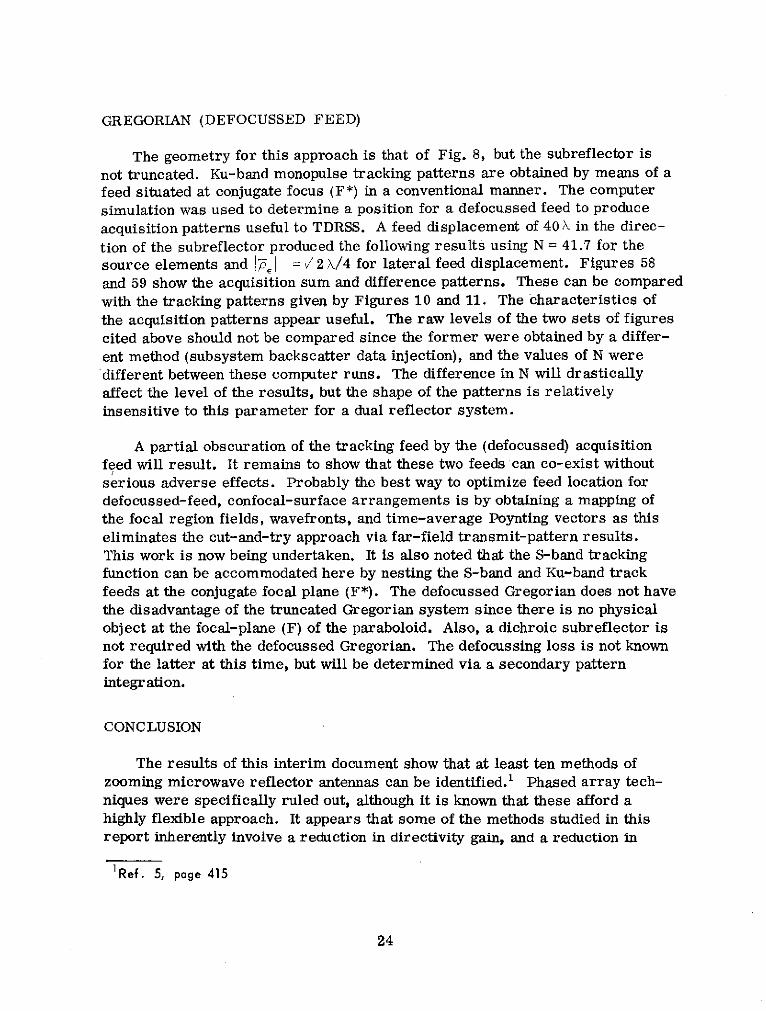
GREGORIAN (DEFOCUSSED FEED)

The geometry for this approach is that of Fig. 8, but the subreflector is

not truncated. Ku-band monopulse tracking patterns are obtained by means of afeed situated at conjugate focus (F*) in a conventional manner. The computersimulation was used to determine a position for a defocussed feed to produce

acquisition patterns useful to TDRSS. A feed displacement of 40 X in the direc-

tion of the subreflector produced the following results using N = 41.7 for thesource elements and IT I = / 2 X/4 for lateral feed displacement. Figures 58

and 59 show the acquisition sum and difference patterns. These can be comparedwith the tracking patterns given by Figures 10 and 11. The characteristics ofthe acquisition patterns appear useful. The raw levels of the two sets of figurescited above should not be compared since the former were obtained by a differ-ent method (subsystem backscatter data injection), and the values of N weredifferent between these computer runs. The difference in N will drasticallyaffect the level of the results, but the shape of the patterns is relativelyinsensitive to this parameter for a dual reflector system.

A partial obscuration of the tracking feed by the (defocussed) acquisitionfeed will result. It remains to show that these two feeds can co-exist withoutserious adverse effects. Probably the best way to optimize feed location fordefocussed-feed, confocal-surface arrangements is by obtaining a mapping ofthe focal region fields, wavefronts, and time-average Poynting vectors as thiseliminates the cut-and-try approach via far-field transmit-pattern results.This work is now being undertaken. It is also noted that the S-band trackingfunction can be accommodated here by nesting the S-band and Ku-band trackfeeds at the conjugate focal plane (F*). The defocussed Gregorian does not havethe disadvantage of the truncated Gregorian system since there is no physicalobject at the focal-plane (F) of the paraboloid. Also, a dichroic subreflector isnot required with the defocussed Gregorian. The defocussing loss is not knownfor the latter at this time, but will be determined via a secondary patternintegration.

CONCLUSION

The results of this interim document show that at least ten methods ofzooming microwave reflector antennas can be identified.' Phased array tech-niques were specifically ruled out, although it is known that these afford ahighly flexible approach. It appears that some of the methods studied in thisreport inherently involve a reduction in directivity gain, and a reduction in

1Ref. 5, page 415

24

spillover efficiency, or a defocussing loss. On occasion both of the latter losses

are a consequence of zooming. The spillover losses appear to be very high

when beamwidth increases of 200 percent or more are required of those systems

that mechanically alter the main or subreflector dimensions. When mechanical

motion is ruled out as a means of achieving zooming, the nested paraboloid

approach is attractive. The Cassegrain and Gregorian systems which utilize

feed defocussing also become attractive when mechanical displacement of

elements is disallowed, however, the analogue nature of the zooming is lost with

the latter.

Whatever system is studied, satisfaction of the monopulse postulates is an

important consideration, and it is inadvisable to analyze the zooming of a pencil

beam only. Geometrical asymmetry, and departure from confocal arrangements,

were found to be nearly synonymous with violation of the postulates, but often

resulted in useful, practical systems. Mapping of the focal region fields was

found to be an indispensable aid in determining monopulse feed location for

variable beamwidth designs. The defocussed Cassegrain and Gregorian systems

should be examined in greater depth with regard to parameters governing source

directivity, lateral displacement, and axial displacement using the three near-field

maps (isophotes, wavefronts, and time-average Poynting vectors). Finally, the

frequency-independent aspects of zooming should be considered. Although the

TDRSS requirements which motivated much of the present effort did not anticipate

significant frequency changes, it is noted that departure from confocal geometry

implies that frequency change will require complete redesign of the zoom system.

This should be contrasted with the nested paraboloid approach, where both

acquisition and tracking functions are wideband.

A search in the Patent Office, Washington, D. C. appears to bear out the

commentary of another investigator' that "there has not been sufficient informa-

tion available to evaluate greatly defocussed antennas for monopulse tracking

operation." Related patents of interest have been collected and are identified

here.

This is an interim report. Work is continuing on the exploration of basic

methods for achieving variable beamwidth or zoom capabilities for microwave

antennas. Among these is the idea of utilizing the first Airy bright ring of a

dual reflector system to obtain a set of low-gain monopulse acquisition patterns.

Another approach is to '"borrow" energy from the periphery of the Airy disc

of a system with a large magnification factor for acquisition purposes, and

then restore this energy, by switching, to the tracking or data mode of operation

after acquisition has been achieved. The results of these efforts are directed

toward relieving the acquisition problems on TDRSS, Space Shuttle, and other

user spacecraft.

IRef. 15

25

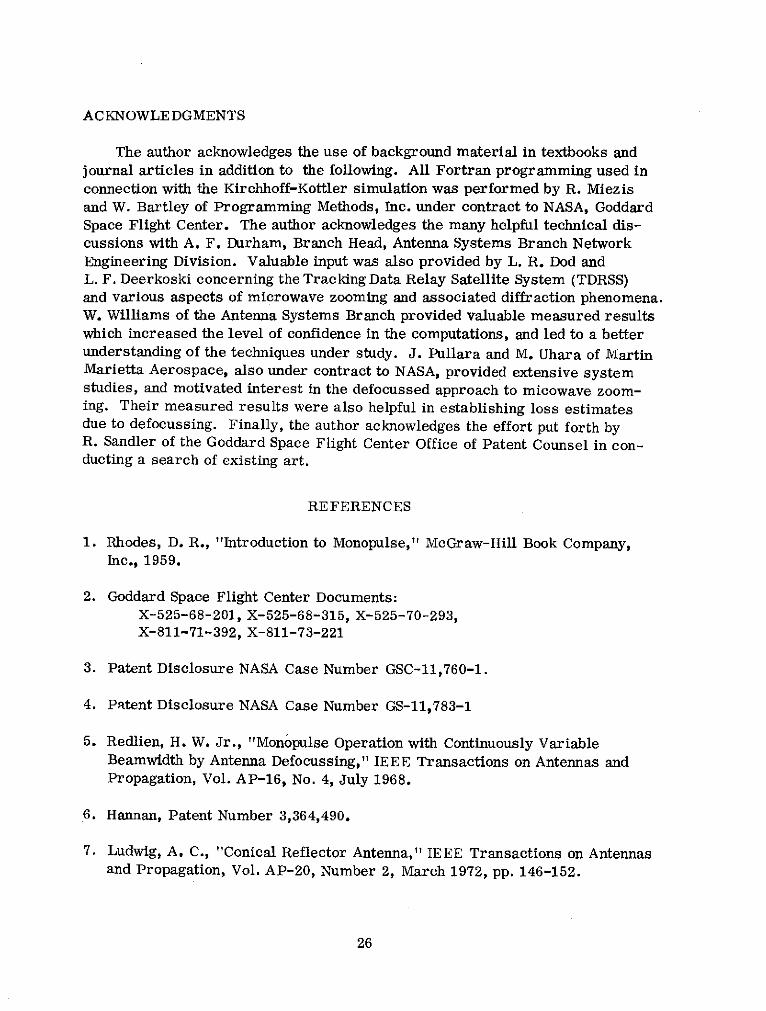
ACKNOWLEDGMENTS

The author acknowledges the use of background material in textbooks andjournal articles in addition to the following. All Fortran programming used inconnection with the Kirchhoff-Kottler simulation was performed by R. Miezisand W. Bartley of Programming Methods, Inc. under contract to NASA, GoddardSpace Flight Center. The author acknowledges the many helpful technical dis-cussions with A. F. Durham, Branch Head, Antenna Systems Branch NetworkEngineering Division. Valuable input was also provided by L. R. Dod andL. F. Deerkoski concerning the Tracking Data Relay Satellite System (TDRSS)and various aspects of microwave zooming and associated diffraction phenomena.W. Williams of the Antenna Systems Branch provided valuable measured resultswhich increased the level of confidence in the computations, and led to a betterunderstanding of the techniques under study. J. Pullara and M. Uhara of MartinMarietta Aerospace, also under contract to NASA, provided extensive systemstudies, and motivated interest in the defocussed approach to micowave zoom-ing. Their measured results were also helpful in establishing loss estimatesdue to defocussing. Finally, the author acknowledges the effort put forth byR. Sandler of the Goddard Space Flight Center Office of Patent Counsel in con-ducting a search of existing art.

REFERENCES

1. Rhodes, D. R., "Introduction to Monopulse," McGraw-Hill Book Company,Inc., 1959.

2. Goddard Space Flight Center Documents:X-525-68-201, X-525-68-315, X-525-70-293,X-811-71-392, X-811-73-221

3. Patent Disclosure NASA Case Number GSC-11,760-1.

4. Patent Disclosure NASA Case Number GS-11,783-1

5. Redlien, H. W. Jr., "Monopulse Operation with Continuously VariableBeamwidth by Antenna Defocussing," IEEE Transactions on Antennas andPropagation, Vol. AP-16, No. 4, July 1968.

6. Hannan, Patent Number 3,364,490.

7. Ludwig, A. C., "Conical Reflector Antenna," IEEE Transactions on Antennasand Propagation, Vol. AP-20, Number 2, March 1972, pp. 146-152.

26

8. Goddard Space Flight Center Document X-811-72-392

9. Cheo, B., "A Solution to the Equiangular Spiral Antenna Problem," Elec-

tronics Research Laboratory, Department of Electrical Engineering.University of California, Contract No. DA 36-039 SC-84923, Nov. 1960.

10. Spencer, Holt, Johanson, and Sampson," Double Parabolic Cylinder Pencil-Beam Antenna," IRE Transactions-Antennas and Propagation, January 1955.

11. Kelleher, Patent Nlumber 3,365,720.

12. Spencer, Patent Number 2,825,063.

13. Goddard Space Flight Center Document X-811-73-221.

14. Patent Disclosure NASA Case Number GSC-11,862-1.

15. Related patents:

Laibson, et al. 3,383,692Kott 3,396,397Bohnert, et al. 2,570,197Tipton 3,176,302Brunner 3,276,022Hersch 3,594,804White 3,230,538Williams, et al. 3,394,378Kelleher 3,354,461

Van Staaden 2,991,473

Ruben 3,504,368Thourel 2,913,723

27

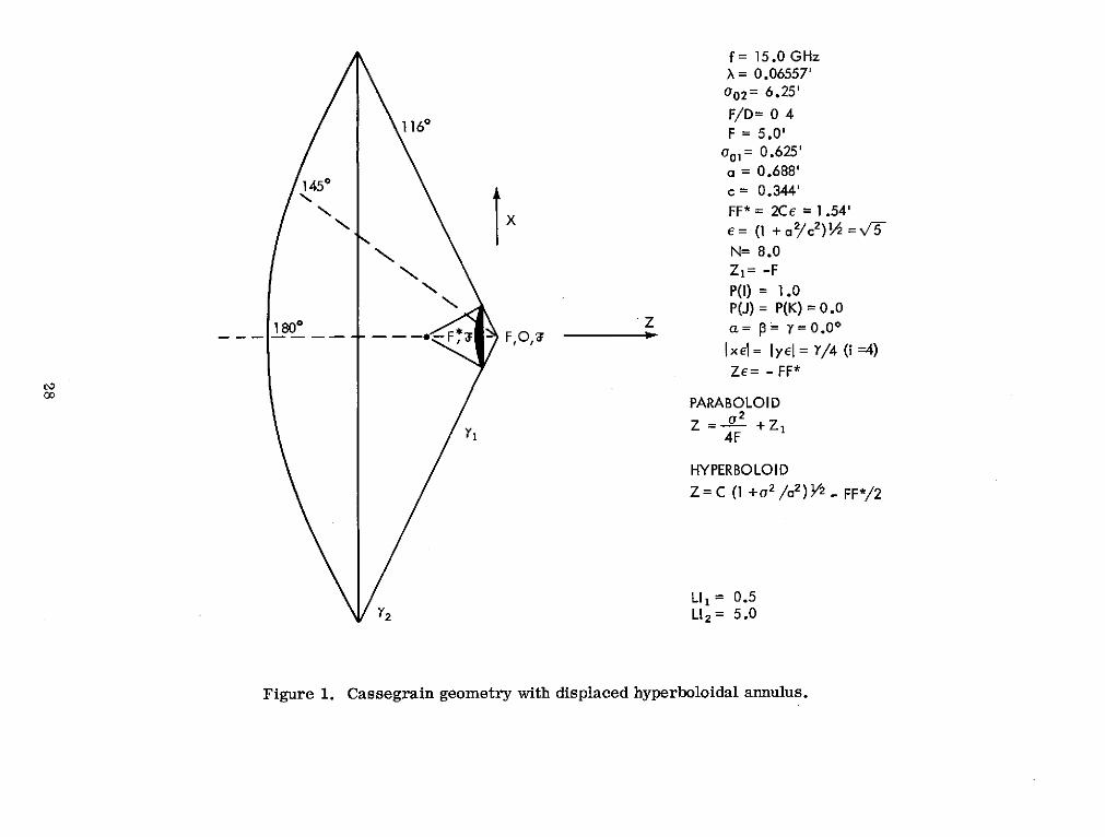
f = 15.0 GHzX = 0.06557'002= 6.25'

F/D= 0 41160 F = 5.0'

o =01 0.625'a = 0.688'

1450 c= 0.344'

FF*= 2Ce = 1.54'X E = (1 + a2/C2 ) =v-

N= 8.0Z 1= -FP(I) = 1.0P(J) = P(K) = 0.0

1800 Z a= p= 7= 0.001800 --- F - F,O, a

Ixl = I yel = Y/4 (i =4)Ze= - FF*

PARABOLOID

Z 0 2 + Z1'1 Z 4F

HYPERBOLOIDZ= C (1 +2 /a 2 ) 2 - FF*/2

LI1 = 0.5Y2 LL2 = 5.0

Figure 1. Cassegrain geometry with displaced hyperboloidal annulus.

db

-40

E MAx MAIN POL SUM PATTERN (1)FULL HYPERBOLOID

-50

deg.

-60 400

-70 300

-80 0* • - 200

-90 - 100

* E4 ***00.

-100 -**** 0

-1100.0 0.2 0.4 0.6 0.8 1.0 1.2 1.4 1.6 1.8 2.0

0 -deg., = 90.0 deg.

Figure 2. Tracking pattern, X-mode.

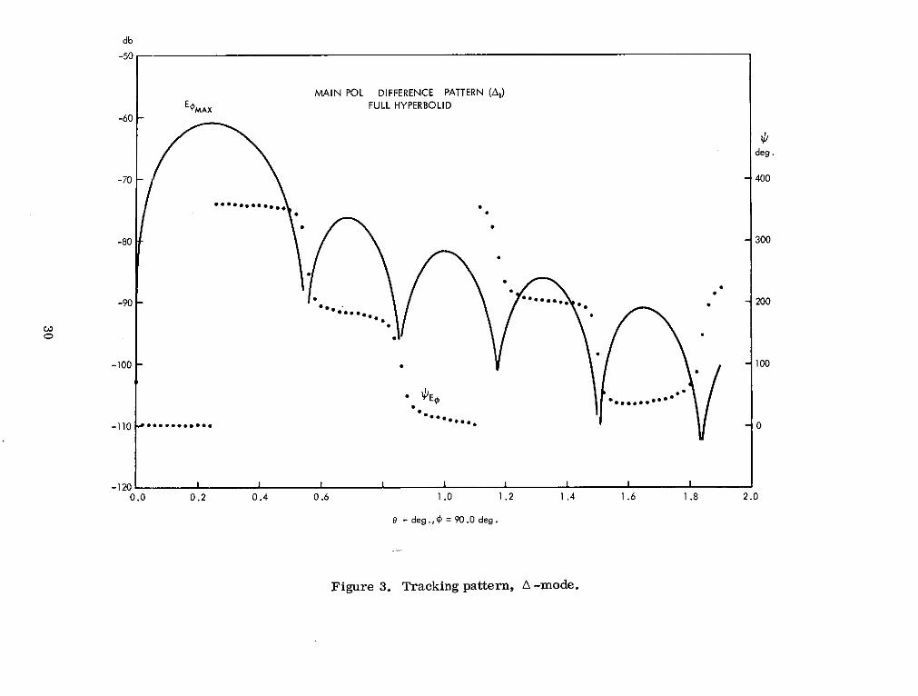
db

-50

MAIN POL DIFFERENCE PATTERN (A1)

E MAX FULL HYPERBOLID-60

deg.

-70 - - 400

-80 300

-90 ** 200

-100 100

-110 ******* ** - 0

-120-120 I I I I I I I I I

0.0 0.2 0.4 0.6 1.0 1.2 1.4 1.6 1.8 2.0

0 - deg., = 90.0 deg.

Figure 3. Tracking pattern, A -mode.

db

-50

E MAx

MAIN POL SUM PATTERN (1)TRUNCATED HYPERBOLOID

-60

deg.

-70 - - 400

-80 - - 300

*9 .* - 200.*

-90 00

-100 100

E I0-110 - - 0

-120 I I I I I I I I0.0 0.2 0.4 0.6 0.8 1.0 1.2 1.4 1.6 1.8 2.0

0 - deg.,O = 90.0 deg.

Figure 4. Acquisition pattern, Y -mode, (truncated hyperboloidal annulus).

db

-60

MAIN POL DIFFERENCE PATTERN (A 1)

E MAx TRUNCATED HYPERBOLOID-70

deg.

-80 - 400

-90 -300

-100 s* 200

S *

... ***".

110 100

-120 * ..... ** *. @ - 0

-130 I I I I I I I I I0.0 0.2 0.4 0.6 0.8 1.0 1.2 1.4 1.6 1.8 2.0

0- deg., = 90.0 deg.

Figure 5. Acquisition pattern, A -mode, (truncated hyperboloidal annulus).

db

-50E MAX

MAIN POL SUM PATTERN (E)DISPLACED HYPERBOLOIDAL ANNULUS (+4 X)

-60 -

deg.

-70 --400

300-80 - 300

* 100-0 - 200

00.04.0 01 - 0

1100-100

-120 I I I I I I I0.0 0.2 0.4 0.6 0.8 1.0 1.2 1.4 1.6 1.8 2.0

0 - deg.,O = 90.0 deg.

Figure 6. Acquisition pattern, I -mode, (S = +4X displaced hyperboloidal annulus).

db

-60

MAIN POL DIFFERENCE PATTERN (Al)E4MAX DISPLACED HYPERBOLOIDAL ANNULUS (+4 X)

-70

deg.

-83 400

-91) 300

*o

*-100 o200

0

-120 S - 100

-1300

-130 I I I I I I I I0.0 0.2 0.4 0.6 0.8 1.0 1.2 1.4 1.6 1.8 2.0

0- deg., = 90.0 deg.

Figure 7. Acquisition pattern, A -mode, (S = +4k displaced hyperboloidal annulus).

N

N II

U)LL. U W LL

x x

/ \

L LI........... C)4

x

Figure 8. Gregorian geometry with truncated ellipsoidal annulus.

35

db

-90

omax. 1.4' PENCIL BEAMS (i= 1.0)1.0'

-100- .8

0.6'

-110 - -. N

0.4' ..

-120 =\.> = % -- \

-130 -

II /-140 II \

I * ..

-150

Note: paraboloid obscured by ellipsoids of radiusomax.

-160 I 1 I0 .2 .4 .6 .8 1.0 1 .2 1.4 1.6 1.8 2.0

0 - degrees , (0 = 0.0 degrees)

Figure 9. Beamwidth versus subreflector diameter for modified Gregorian system.

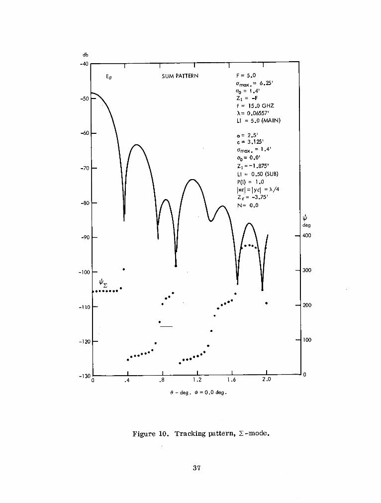
db

-40

EO SUM PATTERN F= 5.0

amax.= 6.25'

ao = 1.4'

-50 - Z1 = -F

f = 15.0 GHZX= 0.06557'

LI = 5.0 (MAIN)

-60 - a = 2.5'c = 3.125'

Omax. = 1.4'

o = 0.0'

-70 - Z, = -1.875'

LI = 0.50 (SUB)P(1) = 1.0

Ixe l yel = X/4Ze = -3.75'

N= 0.0

deg

-90 - - 400

-100 - - 300

-110 * 200

-120 - 100

-130 I I I I 00 .4 .8 1.2 1.6 2.0

0 - deg. 0 = 0.0 deg.

Figure 10. Tracking pattern, -mode.

37

db

-40

EO DIFFERENCE PATTERN

-50 -

-60 -

-70 -

-80

deg.

-90 - - 400

-100 - - 300

0 0

-110 - * oo * - 200

-120 - * - 100

-130 I I I I00 .4 .8 1.2 1.6 2.0

0 -deg., = 0.0 deg.

Figure 11. Tracking pattern, A -mode.

38

db

-50

Subreflector:

Ee SUM PATTERN omax.=0. 74'-60 - Main reflector:

ao = 0.74'

-70

-80

-90 -

deg.

-100 - - 400

-110 - - 300

-120 - - 200

000000

-130 . -100

0 0

-140 0

*000.. 00

-140 I I I I I0 .4 .8 1.2 1.6 2.0

0 -deg. 0 = 0.0 deg.

Figure 12. Acquisition pattern, 2 -mode.

39

db

-50

Subreflector:

amax. = 0.74'

-60 - DIFFERENCE PATTERN 0.74Main reflector:

00= 0.74'

-70 -

Ee

-80

-90

deg.

-100 -400

-110 - - 300

'Ee0000 000 *000 ,0000go000g 0

-120 - - 200

-130 - - 100

-140 _I 00 .4 .8 1.2 1.6 2.0

-265.09 db , = 0.0 deg.

Figure 13. Acquisition pattern, A-mode.

40

640

II

I

I

Fs F O,FM

7K, 7K2

S K1 (TRK)(ACQ)

Pm

Figure 14. Nested Paraboloid Geometry.

41

IEel in db

-50

Eel MODE Large Paraboloid:

F= 5.0'

max. = 6.25',oo= 1.58'

-60 - Z, = -F

LI = 2.0

Small Paraboloid

Eel A MODE F = 1.26'

-70 amax. = 1.58', = 0 40'

Z, = -5.36'LI = 2.0

-80

-90

-100 f =15.0 GHZ,X = 0.06557'

N= 1.40, i=4

IjxI = Iyel = 0.016'Ze = -4.10' kEO

-110 - P(1) = 1.0 - 4000

'E 0 2 MODE* 9OOO*OOO00OOOOO 0 o000000

O

000 - 3000

o - 2000

0 PE A MODE o o000000 0000000000001 **ee 0 0006600

o - 1000

0

I I I 0 I I o

0 1.0 2.0 3.0 4.0 5.0

0 in degrees,1 = 00

Figure 15. Acquisition patterns, I and A modes with main paraboloid.

42

IEe in db

-50

iEel I MODE Small Paraboloid:F = 1.26'omax.= 1.58', ao=0.40'

-60 Z = -5.36'LI = 5.0

IEel MODE-70

-80

-90

-100

VEe

-110 - - 4000

OEg X MODE***** ** O**O 00oooooooo00 oo00 00000000

f = 15.0 GHZ , X= 0.06557' - 3000N= 1.40, i=4

Ixel= lyel= 0.016'Ze = -4.10'

P(l) = 1.0 - 2000Eg A MODE

O oo00000000Ooooo0000000ooooo88******* ***o* *..o O

000

0- 1000

0

0 1.0 2.0 3.0 4.0 5.0

0 in degrees,O = 00

Figure 16. Acquisition patterns, 2 and A modes without main paraboloid.

43

IEel in db

-40

Large ParaboloidF= 5.0

IEe MODE ma. = 6.25' ,00= 1.58'

-50 - Z 1 = -F

LI = 5.0

Small Paraboloid:F= 1.26'

-60 - max. = 1.58',00= 0.40'

Z1 = -5.36'jela A MODE LI =5.0

Hyperboloid:

-70 A= 0.353', C = 0.125'

max. = 0.40',%o= 0.0'

Z = 0.375'LI= 0.30

-80

90

f = 15.0GHZ, X = 0.06557'N= 5.649 , i=4 0

Ixel= Iyel = 0.016'-100- Ze = -0.75' 4000

P(I)= 1.0

0

0 0

o - 3000

,E A MODE 0000000

0oeo° •--0200009.0000000000000000 0000000

O 000.00*00 - 2000

Eg I IMODE * 10000000000000000*0 0 0000000000

000O0

00

0 0.25 0.5 0.75 1 0 1.0.25 1.5

0 in degrees, =0

Figure 17. Tracking patterns, : and A modes with acquisition paraboloid.

44

IEel in db

-40

Large Paraboloid:

F = 5.0'|Ee MODE max .= 6.25' ,ao= 0. 4 0'

-50 - Z = -F

LI = 5.0

HyperboloidA = 0.353', C = 0.125'

-60 -max. = 0. 4 0 ,ao = 0.0'

Z = -0.375'IEeI A MODE LI = 0.30

-70

-80

-90

f = 15.0 GHZ, X = 0.06557' E

N= 5.649 , i=4

-100 I x e = Yel = 0.016' 4000ze= -0.75'

P() = 1.0

0*0

S300

0

* 0 2000

o 200

F Eg MODE k .. o d-e0

:** * E g A M O D E0

0 0.25 0.5 0.75 1.0 1.25 1.5

0 in degrees

Figure 18. Tracking patterns, 2 and A modes without

acquisition paraboloid.

45

640

x

Fl* z

P,

46

IE in db

-50

Paraboloid:

IE8l Z MODE F = 5.0'omax.= 6.25' ,ao = 0.75'

-60 -Z = -F

LI =5.0

Hyperboloid:A= 1.3', C=1.247'

max. .= 0.75',ao = 0.0'

Zz= -FF*/2=-1.802'LI =0.5f =15.0 GHZ,X=0.06557'

N= 77.3 , i=4-80 Ixel = lYEl = 0.0164'

z e = -3.60'1Eg&MODE P(I) = 1.0

-90

-100

-110 - - 4000

s******0**00 oo **ooo

o c0 0

-120- - 300°

***************** 0o o o

0O

0 , 1O00I I I o I I °

0 0.25 0.5 0.75 1.0 1.25 1.5

0 in degrees,P = 0O

Figure 20. Tracking patterns, Y and A modes (N = 77.3).

47

IEel in db-50

HYPERBOLOID:Z, = -FF*/2 - 3X/2

-60 - N = 77.3

IEel Z MODE

-70

-80

-90 - 1Ee A MODE-90

-100

rE0

-110 - 4000

o o o

0 0 .000

0 0

-120 00 - 000

Eo A MODE o000 000

0 0 0

o o

0 0

9 *so o MODE 00 0 0 0

ooO O00 1000

O in degrees, 0 0°

Figure 21. Acquisition patterns, I and A modes (N = 77.3)for AZ = -3k/2 of hyperboloid.

48

db

-50

HYPERBOLOID:Z 1

= -FF*/2 -2 X

-60 N = 77.3

Ee(C)

-70

-80

-90 -

deg.

S400

-110° .' * - 3000

r*

-120 7 00 0 - 200

0 00

-130 . * * - 100

-15o I 00 0.25 0.50 0.75 1.00 1.25 1.50

0 - degrees, = 0.0 deg.

Figure 22. Acquisition patterns, I and A modes (N = 77.3)

for AZ = -2X of hyperboloid.

49

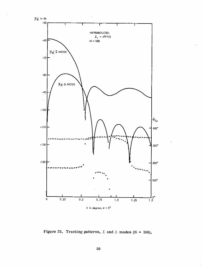
IE in db

-50

HYPERBOLOID:Z 1 = -FF*/2

-60 - N = 100

El I MODE

-70

-80

lEl A MODE

-90

-100

-110 - 4000

ooo oooo oo o oo oo o o o

-120- * 3000

-130 - - 2000

0000 000

I a I0

0 0.25 0.5 0.75 1.0 1.25 1.5

0 in degrees,P = 00

Figure 23. Tracking patterns, I and A modes (N = 100).

50

IEel in db-50

HYPERBOLOID:Z= -FF*/2 - 3X/2

-60 - N= 100

IEo 2 MODE

-70 -

-80 -

IEOl MODE

-90

-100 -

-110 - 4000

0 .0

0 •0 0

-120 0000 00 0

o EA MODE oO

oo 2 00

o • ooo

00

0E A MODE O 0 0_ * o* • 2000

00

0 0

0 0.25 0.5 0.75 1.0 1.25 1.5 1.75

0 in degrees,P = 00

Figure 24. Acquisition patterns, I and A modes (N = 100) for AZ = -3X/2.

51

IEel in db-50

HYPERBOLOID:Z =-FF*/2- 2X

-60 - N =100

IEl Z MODE-70

-80

JE01 A MODE

-90 -

-100 -

Eg

-110 - 400*

0 00

-120 0 o0 30000 *o

o * o

0 o

06oo

60 0 -00 2000

o* o 100Soo 0

: ....... * **

0000 0

0 0.25 0.5 0.75 1.0 1.25 1.5 1.75

0 in degrees , =0'

Figure 25. Acquisition patterns, Z and A modes (N = 100) for AZ = -2k.

52

10"

SCALE

Figure 26. Conical-Gregorian geometry with spiral antenna feed.

53

IE8 I in db-40

N= I a= 1/3

-50 -N=2

-60 - N =3

N=4

-70

-80

-90

-100

-110

-120

I I I I I

1800 1600 1400 1200 1000 90*

0 in degrees, q = 0'

Figure 27. Primary radiation patterns of spiral antenna

(a = 1/3, n = 1, 2, 3, 4).

54

IEel in db-80

Ee N = a= 1/3

-90 -

-100 -

IEl N = 2

-110 -

-120

-130

OEg

-140 - - 4000

'E, N = 2

0000000000000000000 00

0

0 - 3000

0

ooooooooo-2000

IEg N= II0********* .. * -1000

0

00

180 179 178 177 176 175

8 in degrees, 0 = 0'

Figure 28. Tracking patterns, X and A modes, of the Conical

Gregorian System (a = 1/3, n = 1, 2).

55

IEel in db

-110

IEel

-120 -

-130

-140

MAIN REFLECTOR-150 LI = 1.5

SUBREFLECTOR

LI = 0.5

-160

PE0

-170 - - 4000

-180 ,* - 300"

00

180 179 178 4-77 176 175

6 in degrees, 0 = 0

Figure 29. Acquisition pattern, A mode, of the Conical

Gregorian System (a = 1/3, n = 4).

56

tx txPOINT- SOURCE POINT- SOURCE

FOCAL AXIS F OF Y1 SECTOR OF

SPHERICAL WAVE

2/ I ACTUAL RAYSINTERSECTION / \

OF Y ANDY2 SECTOR OF/ PLANE WAVE

S\ I INTERSECTION OF 1 AND Y2

\ VIRTUAL RAYS t2+ F/ \ I 4Fcl

/ \ I y=t

SECTOR OF VIRTUAL I 1 Ft

IPARENT CYLINDRICAL WAVE I z 4 F - FC2IPARABOLIC CYLINDER PARENT

S z Y z PARABOLIC CYLINDER

FOCAL AXIS IOF Y2

Figure 30. Dual parabolic cylinder geometry.

db

-120

CHANNEL I SUM PATTERN

-130 EO (MP)

-140 -

-150 -

-160 -

deg.

-170 A i E E 400

O0-180 . 300

-190- . • , 200

-200 T • • • • Too

-210 030 20 10 0 10 20 30

8-ceg. 0 -deg.

0 = 0 deg. =180 deg.

Figure 31. Acquisition pattern, Channel I (2).

db

-120

CHANNEL I DIFFERENCE PATTERN

-130

EO (MP)

-140 -

-150-

-160

deg.CTICO -170 -

-400

-180 300

- 19 0 - a a 2 0 0 •

-200 - 00 0 0 0 -100

-21 I I I I 1 1 *30 20 10 10 20 30 0

0-= Odeg. -deg.

SOdeg. = 180 deg.

Figure 32. Acquisition pattern, Channel I (A).

db

-120

-130 E (MP) CHANNEL II SUM PATTERN

-140

-150

Ep (CP)

-160

deg.

-170 E 400

°-180 -300-180•

-190 - * - 200

-200 C - 100

0.

.

-210r I I * I00 10 20 30

e -deg., =90

Figure 33. Acquisition pattern, Channel II (s).

60

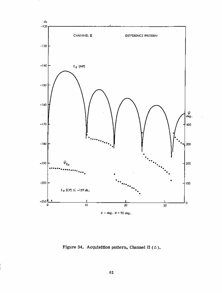
db

-120

CHANNEL II DIFFERENCE PATTERN

-130

-140 - Eg (MP)

-150

-160

deg.

-170- 400

-180 -* 300

-190 - E6 * 200

-200 -... 100

E (CP) -159db. .

-210 I I00 10 20 30

0 - deg. 4 = 90 deg.

Figure 34. Acquisition pattern, Channel II (A).

61

db

-100 III

CHANNEL I SUM PATTERN

-110

-120 - Eo (MP)

-130 -

-140 -

deg

-150 400

m soE g Eg

-160- - 0 300

-180 - 00

-190 - 0 100

15.0 12.5 10.0 7.5 5.0 2.5 0 2.5 5.0 7.5 10.0 12.5 15.00

S- deg. 0 -deg.

0deg. = 180 deg.

Figure 35. Tracking pattern, Channel I (2).

5*~~ 0I 5

Figure 35. Tracking pattern, Channel I (1.

db

-100 I I

CHANNEL I DIFFERENCE PATTERN

-110

-120 -

Eo (MP)

-130 -

-140 -

deg.

-150 - 400

-160 -* , * * s * * - 300

-170 -

-1 80 0 *

-1* *-1 0 •*S•• 2 *

-19 . l .1 I 1 I 5. " I 0 I I f l o

15.0 12.5 10.0 7.5 5.0 2.5 0 2.5 5.0 7.5 10.0 12.5 15.0

, - deg. 0 -deg.

S= 0 deg. 0 = 180 deg.

Figure 36. Tracking pattern, Channel I (A).

IEel in db-120

Eel (MP) CHANNEL I SUM PATTERN

-130 -

-140 -

-150 -

-160 -

-170

400

* * - 300

Eo

- 200

• o*

S100

1 I I I I 00 2.5 5.0 7.5 10.0 12.5 15.0

8 - degrees , = 90

Figure 37. Tracking pattern, Channel II ().

64

db

-100 I I I

CHANNEL II DIFFERENCE PATTERN

-110

-120

Ee (MP)

-130

-140

deg.

-150 - 400

so

-160 - ° - 300

-1700 -gEg 2

-190

0 2.5 5.0 7.5 10.0 12.5 15.0

0 -deg., = 900 , 2700

Figure 38. Tracking pattern, Channel II(A).

65

23/I

22

21

/

20

S19i

16z

z 18

17

-5.00 -4.00 -3.00 -2.00 -1.00 -0.00 1.00 2.00 3.00 4.00 5.00Z IN WAVELENGTHS

Figure 39. Electric-field distribution (ACQ).

66

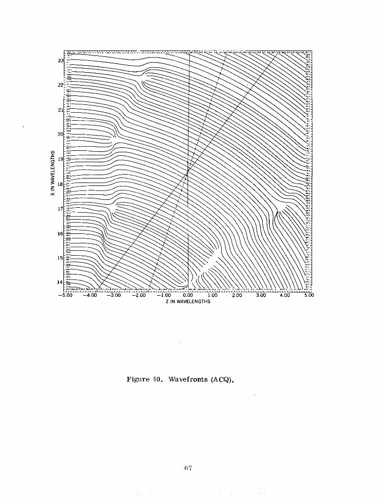
23

22

21

cn

' 19

18

17

16:

15

14

-5.00 -4.00 -3.00 -2.00 -1.00 0.00 1.00 2.00 3.00 4.00 5.00

Z IN WAVELENGTHS

Figure 40. Wavefronts (ACQ).

i 7

S iiii i i~~iiiiii~ i ii!!! iiiiiiiii i ii~ i Ii i i i (Iii i i i i i i i i ;! i i i i ii~ ii iiii iii~ ii? [!ii~ iii ??i ii?? i227 ii) :: ; : i : : t ; : : ; ; ; ; ; , ; :!:::::: ;:::

.:::::::::::

2lii ji jiiijiiijjiiii i i ii i i i i iiii i jjI )i i ii i iii ~~iii

.. .... .. ... ..... .. .. .. .. .... .. .. .... ... .. ... .. .. ... .. ....:: : : : :: : : : : : : : :

...................... ...... ... it~~l~~t~~l~~i, H. .... ..,. ... .... ,I I ~ ¢ / tt t t t

20 ~~~~ ~ . .. . . . . . .... ..... ... .. ........ ...,.,, ,,... ...... ,...... ..iifl. Y...T .... T t.................... .

i I 1 1 1 / I f t t t r , . . ., r l l. . . . . . . . . . . ..II I

Ii~~~fl~~irl *t~~~~~l. .........ttl t/ ........ ll l l/ lt t . . .. . .. .

9l l \ItI I I It ... ............ . . . .... . . . ,,,,, .. .... ,,................ ....

20

i i i il i i i i I . ii iitii Ii I I i I i I I I I I III I]~ 1 It III IIIII II II l t l l l l t, # ...... .... :

9 ................... ....... ..... ... .... . ....... . ..... .IIIII ~ ftl fl~ l ... ill /I Il llll It IIII ~ t I ~ llll ltlt t//t ......... ..... . . . .,

ll ft ~ f ~ l t~ l ,, l ft Il tt tl t lll lt t /l /l/ lt /t............t .. .. .. ..

14,

.. ' '

I I ' ' '

. . . . . . .... l l , , , , ... . . . . . . . . . . . . . . . . . . . . . . . . . . ./ t t / t z l t / , . . . . . . . . . . .

................................ ...... .. . . . . . . . . . . . . . . . . .. . . . . . . . . . . . . . . . . .'.. . . .t / / l l l / / t r l l . . . . . . . . . . . . . . . .........~ t ,I, . .... ....................... // // I/ // # / /i tl t.. . .. .. .. .. ...... .............. ................ . ;,, ; ,; ; ; ; ; ; ,:. ... ... .

................ ............. ..... . .

'E ii i~:::j l::j:gi2 i 22? : ii !iiiii : ? iiiiii ii1i 1i5 ?i?!:

18,8

;; : Z : . .. .. .. ................. .. . . .. . . .................

.. .. . .. .. . .......... . . ..... ... ....:: :: : : : : : : : : :: : : :: : : : : : :: : : : : :

14 ~ ~ ~ ~ ~ ~ ~ .... ...::::i'',;;;;;;;; ;; :::i] .. . .. ....... .. ..

II

-... .. .. .. .. .. .. .. .. .

_ 18

1 7 . . . . . .. . .. . . . . . . . . . .

16. . . . . . . . . : . . 1 . . . .

.....; 5 ... .. .. . . . . .. . ... .14. . . . . . ...: : - " " . ... . . . . . .

.5...4.....O.-.0.-.0 .0. . 0 2.....0 3 . . 0 5.00,,' -',- ,...~~ ~ ~ IN........ WAVELENGTHS.................

Figur 41. ime-aerag.Poyning.vctor (AQ......

68. .... ...... ....

23 I

/I/

21

.1817

1718

14 /

-5.00 -4.00 -3.00 -2.00 -1.00 0.00 1.00 2.00 3.00 4.00 5.00Z IN WAVELENGTHS

Figure 42. Electric-field distribution (TRK).

69

16

17~~~~1 ~~~~-------- ~ h \ \l~\ \ l\ \

14

-5.00 -4.00 -3.00 -2.00 -1.00 0.00 1.00 2.00 3.00 4.00 5.00Z IN WAVELENGTHS

Figure 43. Wavefronts (TRK).

70

23

::::::::::::::::::::::::::::::::::::::::::::::: ....... .. ................22:::::::::::::::::::::::::::::::::::::::::22 ...................................................................... ..........i i ..

2 1 ..........

. . . .... ... ...... .. ... ... ..... ..

202 0 : ................. ... ........... ... . ...... ..., ,1,9 ', ..... .......... .. . .. . , , ............. ............. .....

C 19

.iiiiiiiii.. .....ii. .i l. . .. .

z 18

1 5: : : : . .. .. ... .. .. ...... .. ....... ... ... .. ... ....

Sj j j i i - !i i iiiii i i i ii ii ii ii _____________

14 .. ... ...............

-5.00 -4.00 -3.00 -2.00 -1.00 -0.00 1.00 2.00 3.00 4.00 5.00

Z IN WAVELENGTHS

Figure 44. Time-average Poynting vectors (TRK).

71

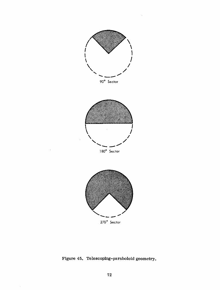
I

900 Sector

I

1800 Sector

2700 Sector

Figure 45. Telescoping-paraboloid geometry.

72

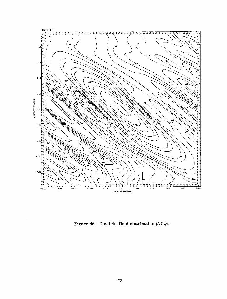
ZYET IN DB

4.00

3.00 "

2.00

1.00(

0.00 -a

,rr no a as

-1.00

s

-2.00:,:: o

21

-3.00

-5.00 -4.00 -3.00 -2.00 -1.00 0.00 1.00 2.00 3.00 4.00 5.00Z IN WAVELENGTHS

Figure 46. Electric-field distribution (ACQ).

73

AYET IN DEGREES

3.00

2.00

1.00

0.00z,

z

-1.00

-2.00

-3.00

-4.00

-5.00 -4.00 -3.00 -2.00 -1.00 -0.00 1.00 200 3.00 4.00 5.00

Z IN WAVELENGTHS

Figure 47. Wavefronts (ACQ).

74

AYET IN DEGREES

" " " " " " " " " " ' "' .................... "'" "'" " \\ " " ............. ...... " " ' " '" " " " " " " "

. ......... ..........'" " " "" " " "" "'""'"

4.00 ............... ...........

" " " " "\ " "' " " ''' ............ ...... ....... *''' "'" ' '" "'' '

"""" \ \\\ L\""" '''"'"'' ''' '' ' ''" ............ ''''''

""" " \ \" \\ \ "'' "''''''''' '' '............... ......'''''' '................................ '' ' "'''' " " ' '''''" ' ''

3.00- .......... ............ ''''''' ''' ' ' '' ''' '' '''""" "" \" \............... ....... '' " " '" " " ''' " "" ' ''""""" \" \\ \ \\ ................ ' '

--------------- - - - - ,- - ........... " '" ' '''' " " " ''-------------- ... _ _ .. ............ ' ' ' "'''' " " ''

------ ------ ------" \ \ \ \ \

1.00 -- -- ...... ------------ ............. ;; ;~, \

-- - - - --- - --- --- - - - -- - - - - -- - - -- - - - z . . . . . .. . . . . . . . ..~ ----~~--- -- . . . . . . .. . . . . .\

0.00: ............... Z--~\~\ ~,,. .~,~,.~..~~~.~. ~..~~......... z .. .. . . . . . . . . . . . . . . . .. . . ..

L """"""""" " . . . . . . .. .. .. . . '

. . . . . .. .. . . . . . .. . . . . . . . .. . . . . . . . . . .... . ... I

z .,..,.. . . . . . . . . . . . . - - - - - - -- - - - --- - -- - - - - --,~.

~ ~~~~~~\------------------... ~ .. ~. .. ~. ~ ~ ~ ~ .................~. ---

. . . . . . . . . . . . .. . . . . . . . .. .------. . . . . . . . . .. . . . . . . . . . . . . . . . . . . . . .. . . . . .- -

' ' . . . . . . .. . . . . . . .. . . . . . . .. . .. . . . . ..,. .. _~~~~~~~~ ~''' ' ''' ' '' ' ., ,,, .,,. ~\\\\\\\\\\\..............-----

" '' " " " ' ' ................ . .................. ..........\\\"'' " '' \\~\\\\\\\~................~----

. . . . . . .. . . . . .. . . . . . . . . . . . . . . . . . . . .. . . . . . . . .. . ... . . .. . .. . . . . . . . . . . .. .. . .. . . . . ...~~.~. .. ,~,, ,,,,,,, ,,,. .,.........~~.

r . . . . . . . . . . .~.. . . . . . . . .. . . . . . . . . ,~~.-5.00 -4.00 3tt _2. I.O O' __Ol . . . . . . . . . . 2tt 1M 4.M .5L

. .... ... ,Z IN WAVELENGTHS...~~~

Figure 48. Time-average Poynting vectors (ACQ,, ... ,,.,.,..,.,). .......

.. . ........ ~ .......... ,,,,,,,.,,,,75,,~,

db

CHANNELI SUM PATTERNEO (MP)

-50 -

-60 -

-70

-80

deg

-90 - - 400

* e *

-100 - * * - 300

-110- *, * " - 200

-120 100

-130 I I I I I I I I I " I I 01.50 1.25 1.00 0.75 0.50 0.25 0 0.25 0.50 0.75 1.00 1.25 1.50

0 - deg. e - deg.

= 0 deg. O= 180 deg.

Figure 49. Acquisition pattern, Channel I (2) ( < = 00, 1800).

db

-4O I I I II

CHANNELI DIFFERENCE PATTERN

-50 -

-60 - E (MP)-60

-70 -

-80 -

deg.

-90 - - 400

-100- * - 300

O l , o o* *

-110 1- * - 200

Ole

-130 I *I I I I 0 I I I 6 1 1 01.50 1.25 1.00 0.75 0.50 0.25 *0 0.25 0.50 0.75 1.00 1.25 1.50

0 -deg. 0 -deg.•= deg. = 180 deg.

Figure 50. Acquisition pattern, Channel I (A (q= 0, 180').

db

-40

E6 (MP) CHANNEL I SUM PATTERN

-50

-60

-70

-80 /

deg.

-90 - 400

-100 -300

-110 -200

-120 - 100

-130 I I I I I 00 0.25 0.50 0.75 1.00 1.25 1.50

0 - deg., 0 = 90 deg.

Figure 51. Acquisition pattern, Channel I (f) ( = 900).

78

db

-40 I I I I I

E0 (MP) CHANNEL I DIFFERENCE PATTERN

-50 -

-60-

-70 -

-80 -

deg

-90 - 400

-100 - 300

-110 - - 200

-120 - - 100

-130 1 I I I I 00 0.25 0.50 0.75 1.00 1.25 1.50

0 - deg.,4 = 90 deg.

Figure 52. Acquisition pattern, Channel I (A) ( = 900).

79

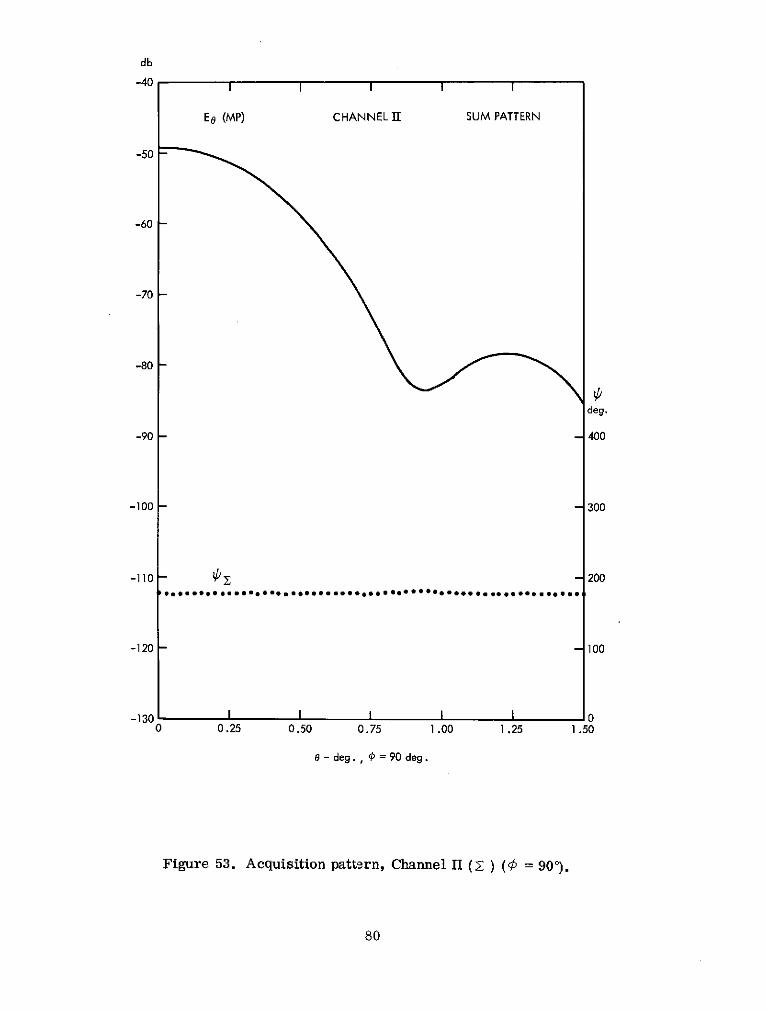
db

-40 I I I I I

Ee (MP) CHANNEL II SUM PATTERN

-50

-60

-70

-80

deg.

-90 - - 400

-100 - - 30

-110 - - 200

-120 - 100

-130 I I I I00 0.25 0.50 0.75 1.00 1.25 1.50

0 - deg. , 4 = 90 deg.

Figure 53. Acquisition pattern, Channel II (~ ) ( = 900).

80

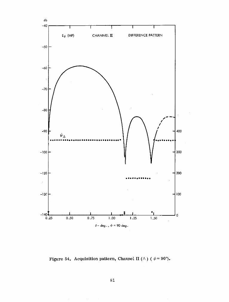
db

-40

E0 (MP) CHANNEL II DIFFERENCE PATTERN

-50

-60 -

-70

-80

-90 -400

-100 - - 300

-120 - - 200

0.25 0.50 0.75 1.00 1.25 1.50

0 - deg., 0= 90 deg.

Figure 54. Acquisition pattern, Channel II (A) ( = 900).

81

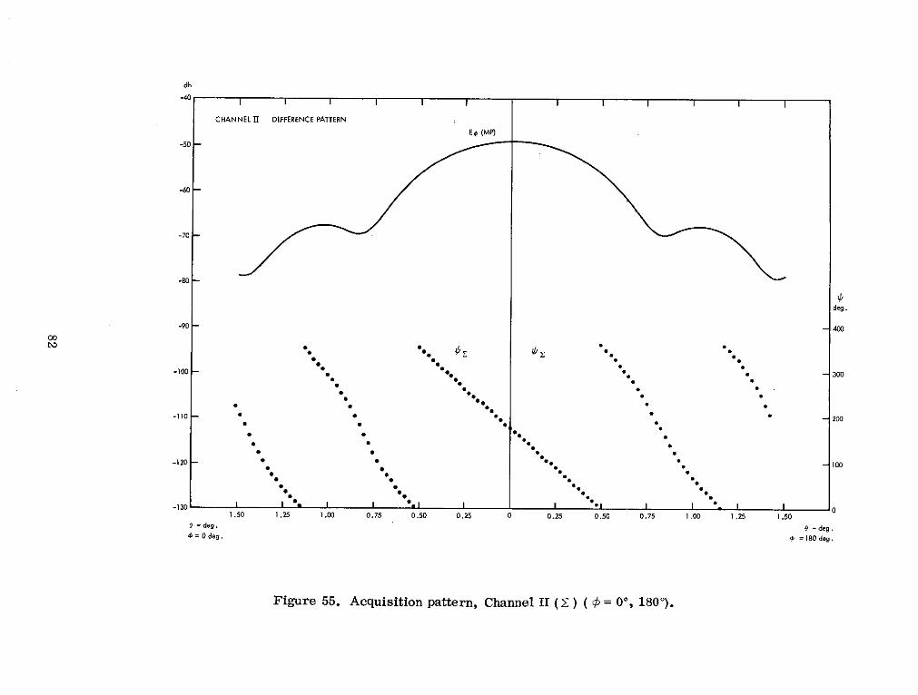
db

-40

CHANNEL 11 DIFFERENCE PATTERN

E 0 (MP)

-50 -

-60 -

-70 -

-80

deg.

-90 - 400

000 °

-100 0 -* 300

* S*

-120 - 1 O00* 0

0

-110 - o - 00

1.50 1.25 1.00 0.75 0.50 0.25 0 0.25 0.50 0.75 1.00 1.25 1.500 -deg 0 -deg.0 = 0 deg. =180 deg.

Figure 55. Acuisition pattern, Channel II ( (= 0, 180).

Fiue55 cuiiin0atrn hnnlI (0)(¢=0 ,10)

db

-50

-60 -FEED POSITIONZe = -FF* + 30

Ixel = lyel= X/4Ee () N = 77.3

-70 -

-80

-90

-100 -

deg.

-110 - 400

-120 - - 300

-130 - - 200

-140- - 100

-150 I I I I I 0

0 0.25 0.50 0.75 1.00 1.25

0- deg.,O = 0 deg.

Figure 56. Acquisition pattern (2) of defocussed Cassegrain.

83

db

-50

-60 - FEED POSITIONZe = -FF* +30X

Ixel = lyel = X/4N = 77.3

-70

-80 -

Ee (A)

-100

deg.

-110 - 400

-120 - 300

-130 - - 200

-140 - 100

-150 I 00 0.25 0.50 0.75 1.0 1.5

0 -deg., O=0 deg.

Figure 57. Acquisition pattern (A) of defocussed Cassegrain.

84

IEel in db

-110

-120

-130 -

-140 - FEED POSITIONze = -FF*+40

IxEl = lYel =/4

N = 41.7

-150

4E0

-160 - - 4000

-170 - * - 3000

- 2000

*

S- 10000

0

I I 00* I I 00

0 0.4 0.8 1.2 1.6 2.0 2.4

0 in degrees,O = 00

Figure 58. Acquisition pattern (2) of defocussed Gregorian.

85

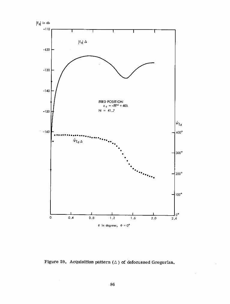
IEel in db

-110

IEl ,A

-120

-130

-140

FEED POSITIONz e = -FF* + 40X

-150 N = 41.7

OEe

-160 - 4000

°o o 02000

1000

- 00

0 0.4 0.8 1.2 1.6 2.0 2.4

0 in degrees, 0 =00

Figure 59. Acquisition pattern (A) of defocussed Gregorian.

86