Embed Size (px)
DESCRIPTION
Economics paper about labor
Citation preview

No. 14-16
Labor Market Polarization Over the Business Cycle
Christopher L. Foote and Richard W. Ryan Abstract: Job losses during the Great Recession were concentrated among middle-skill workers, the same group that over the long run has suffered the most from automation and international trade. How might long-run occupational polarization be related to cyclical changes in middle-skill employment? We find that middle-skill occupations have traditionally been more cyclical than other occupations, in part because of the volatile industries that tend to employ middle-skill workers. Unemployed middle-skill workers also appear to have few attractive or feasible employment alternatives outside of their skill class, and the drop in male participation rates during the past several decades can be explained in part by an erosion of middle-skill job opportunities. Taken together, these results imply that a formal labor market model relating polarization to middle-skill employment fluctuations should include industry-level employment effects and a labor force participation margin as well as pure job-search considerations. The results thus provide encouragement for a growing literature that integrates “macro-labor” search models with “macro-macro” models featuring differential industry cyclicalities and convex preferences over consumption and leisure.
JEL Classifications: E24, J22, J23, J24, J62, J63, J64
Christopher L. Foote is a senior economist and policy advisor in the research department at the Federal Reserve Bank of Boston. His e-mail address is [email protected]. Richard W. Ryan is in the department of economics at the University of Michigan-Ann Arbor, where he is working on his Ph.D. His e-mail address is [email protected] This paper is forthcoming in the 2014 NBER Macroeconomics Annual. For helpful comments, the authors thank, without implicating, the editors (Jonathan Parker and Michael Woodford), the discussants (Richard Rogerson and Fatih Guvenen), Daron Acemoglu, David Autor, Ryan Michaels, Claire Reicher, Paul Willen, and seminar participants at a number of institutions. Thanks are also due to Autor, David Dorn, and Melanie Wasserman for sharing their occupational classification codes. Matthew Curtis and Ryan Ruxlow provided outstanding research assistance. Any remaining errors are our own.
The analysis and results are intended to stimulate discussion and critical comment. The views expressed herein are those of the authors and do not indicate concurrence by the Federal Reserve Bank of Boston, by the principals of the Board of Governors, or the Federal Reserve System. This paper, which may be revised, is available on the web site of the Federal Reserve Bank of Boston at http://www.bostonfed.org/economic/wp/index.htm. This version: December 26, 2014

1 Introduction
A recurring question for macroeconomists and policymakers is how low-frequency employ-
ments trends affect cyclical employment fluctuations for different groups of workers. In the
U.S. labor market, a fundamental long-run trend is polarization, which describes the relative
growth of high- and low-skill job opportunities and the decline of middle-skill jobs.1 As seen
in the decadal Census data at the top of Figure 1, after 1960 the share of nonagricultural
middle-skill jobs began a protracted decline that mimicked the drop in agricultural jobs in
the first half of the twentieth century.2 Polarization stems from two complementary forces.
One is automation, which occurs when machines or computers replace workers in occupations
performing routine tasks, like assembly-line work or clerical jobs. A second polarizing force
is international trade, which allows firms to offshore jobs involving routine tasks to coun-
tries where wages are lower. Jobs in the middle part of the skill distribution are thought to
be particularly vulnerable to automation and trade, for the reason that these jobs tend to
involve more routinized tasks than high- or low-skill jobs.
A possible link between long-run polarization and recent cyclical job losses is evident in
Figure 1, Panel B, which plots indexed employment levels by skill during and after the Great
Recession. Employment growth for high-, middle-, and low-skill workers slowed markedly
during the recent recession, but only the middle-skill group experienced a sharp and last-
ing employment decline. It is reasonable to speculate that middle-skill job matches, which
have the least encouraging long-run prospects, would be the most quickly dissolved when a
recession occurs. As the New York Times put in it 2010:
“For the last two years, the weak economy has provided an opportunity for em-
ployers to do what they would have done anyway: dismiss millions of people—like
file clerks, ticket agents and autoworkers—who were displaced by technological
advances and international trade. The phasing out of these positions might have
been accomplished through less painful means like attrition, buyouts or more
incremental layoffs. But because of the recession, winter came early.3
Modern models of the labor market can formally incorporate the idea that workers with
poor long-run prospects will be the first to be let go when a recession occurs. In these
1Examples of empirical and theoretical work on polarization include Autor, Levy, and Murnane (2003),Autor, Katz, and Kearney (2008), Goos, Manning, and Salomons (2009), Autor (2010), Acemoglu and Autor(2011), and Autor and Dorn (2013). Recent papers on the cyclical aspects of polarization include Fabermanand Mazumder (2012), Jaimovich and Siu (2013), Smith (2013), Tuzemen and Willis (2013), and Corteset al. (2014).
2The Census data are from IPUMS (Ruggles et al. 2010) and make use of its 1950 occupational classi-fication code (OCC1950). We provide more details of the classification of nonagricultural employment intohigh-, middle-, and low-skill jobs in the next section.
3Catherine Rampell, “In Job Market Shift, Some Workers Are Left Behind,” New York Times, May 12,2010, p. A1. Available at http://www.nytimes.com/2010/05/13/business/economy/13obsolete.html.
1

models, workers and firms maintain job matches as long as doing so is in the best interests
of both parties (Mortensen and Pissarides 1994; Pissarides 2000). A long-term decline in the
productivity of a match reduces the value of preserving the match, so a productivity decline
moves the match closer to the margin of being dissolved. Even a small negative shock can
then cause the joint surplus accruing from the match to fall to zero and the match to be
destroyed. After this occurs, the worker can either begin a new job search or use his time in
some other way.
Although a standard search model augmented with long-run employment trends can po-
tentially explain the large middle-skill job losses experienced during more recent recessions,
such a model may not be consistent with other relevant facts. In this paper, we generate
three sets of empirical findings that can help guide the development of formal models of oc-
cupational employment fluctuations. We start by asking a basic question: how do recessions
typically affect employment in various occupations? Because the Bureau of Labor Statistics
(BLS) does not maintain consistent occupational data before the early 1980s, we use con-
temporary BLS publications to construct a new dataset of occupational employment that
begins in the late 1940s.4 We find that the cyclicality of employment for those middle-skill
workers engaged in manual tasks has been both high and stable throughout the postwar era.
Because these manual middle-skill workers are disproportionately employed in manufacturing
and construction—two highly cyclical industries—their high and stable cyclicality suggests
that industry designations matter at least as much as occupational ones for cyclical employ-
ment movements.5 For the other group of middle-skill workers, who tend to perform sales
and clerical tasks rather than manual ones, employment has become more sensitive to the
business cycle over time. Although it is possible that this increase in cyclicality is related
to worsening long-run prospects for this middle-skill group, the employment of high-skill
workers, who have been favored by long-run trends, has also become more cyclical over time.
Our second set of facts concerns the relevant alternatives for middle-skill workers who
become unemployed. These alternatives are crucial inputs into formal search-based models
of the labor market because these alternatives help determine the joint surplus that can
be achieved from continued employment and thus the likelihood that any given match will
be destroyed. Using individual-level data from the Current Population Survey (CPS), we
measure the probability that an unemployed middle-skill worker will transition to a new job
or to labor market nonparticipation, holding constant a number of relevant covariates such
4As we discuss below, the occupational classifications in this dataset are based on those suggested byJaimovich and Siu (2013), who created a historical dataset of occupational employment that begins in the1960s.
5As discussed below, the importance of industry designations for job stability is borne out by separateworker-level evidence on job separations from the Current Population Survey. Flows of middle-skill man-ufacturing and construction workers into unemployment “spike” much more in recessions than they do formiddle-skill workers employed outside of those two sectors.
2
education, age, and the state of the business cycle. We find that middle-skill workers who lack
college degrees rarely end their unemployment spells by taking either high- or low-skill jobs.
Leaving unemployment for nonparticipation is thus a common outcome for those middle-skill
workers who do not return to middle-skill jobs.6 Of course, using matched worker-level CPS
data to study movements from unemployment into nonparticipation has some disadvantages.
In particular, transitions from unemployment to nonparticipation in one month are often
reversed in the following month, when the nonparticipating worker resumes her job search
and is counted as unemployed once again. Consequently, because we do not follow workers
across three successive months, we do not know how many movements from unemployment
to nonparticipation will turn out to be persistent.
Some suggestive evidence for a link between polarization and persistent nonparticipation
appears in Panel C of Figure 1. The participation rate for prime-age males has declined
steadily since the early 1960s, about the time that polarization began. Our third strand of
analysis examines polarization and nonparticipation from a different perspective—by asking
whether groups that have traditionally specialized in middle-skill work are disproportionately
responsible for subsequent declines in participation rates. Our empirical model is based on
one that Acemoglu and Autor (2011) used to study wages; we show that this model can easily
be adapted to study polarization and participation. Estimating the model on males, we find
that the demographic groups specializing in middle-skill work in the late 1970s have much
lower participation rates today. In fact, the model implies that the ongoing decline in middle-
skill job opportunities goes a long way in explaining the decades-long drop in participation
rates among prime-age males.7 In any event, the empirical relationship between polarization
and nonparticipation points to a lack of employment alternatives for a nontrivial share of
middle-skill workers, and thus a lower probability that these workers optimally separate from
their jobs in recessions to search for alternative employment.
All in all, the data suggest that models capable of explaining occupational employment
cyclicality must extend beyond the standard search framework. To understand why middle-
skill employment is so cyclical, one first must understand why manufacturing and construction
output moves so much over the business cycle. Incorporating a volatile investment sector
into a labor market model could be helpful here, given the importance of manufacturing and
construction to the output of investment goods. Additionally, because exits to nonpartici-
pation appear at least as important to unemployed middle-skill workers as exits to high- or
low-skill jobs, a formal model of middle-skill job matches should encompass this margin, per-
6We are unable to tell whether the workers in our dataset who do return to middle-skill jobs resume theirprevious jobs. Below we discuss work by Fujita and Moscarini (2013), who show that unemployed workersoften return to their former employers. Such returns might be especially frequent for middle-skill workers involatile industries.
7Our finding that rising nonparticipation is related to polarization is consistent with Cortes et al. (2014)and Aaronson et al. (2014), which are discussed in the conclusion.
3

haps by allowing nonparticipating middle-skill workers to enjoy leisure or by characterizing
their decisions to get new training. Our empirical results therefore encourage the further de-
velopment of a new literature that blends “macro-labor” search frictions with components of
“macro-macro” models, such as nominal frictions and convex preferences over consumption
and leisure.8
2 The Historical Cyclicality of Occupational Employment and Unemployment
2.1 Data
Official occupational data on employment levels and unemployment rates are available from
the BLS only after January 1983 and January 2000, respectively. Earlier data are not available
because the government’s occupational designations change every 10 years or so, and BLS
officials are not comfortable extending the series corresponding to current occupations further
back in time. Yet it is possible to construct longer time series by using contemporary labor
market reports published by the BLS and the Census Bureau. Soon after World War II,
regular Census reports on the labor force included occupational employment levels for the
first month of each quarter. Monthly data become available in January 1958. Because
occupational data are available only for January, April, July, and October before January
1958, the seasonal properties of a quarterly employment dataset will change when all 12
months become available. We therefore take account of the 1958 break when seasonally
adjusting the data, as explained in the online appendix. Our dataset runs from 1947:Q3 to
2013:Q4.
As pointed out by Jaimovich and Siu (2013), who previously conducted a similar exercise,
the early occupational data can be aggregated into four broad groups based on routine versus
nonroutine and cognitive versus manual distinctions.9 Table 1 shows that the nonroutine
cognitive group consists of high-skill workers performing managerial, technical, or professional
tasks. At the other end of the skill spectrum are low-skill service occupations, such as
cooks and waiters, security guards, groundskeepers, and janitors. The nonroutine nature of
tasks performed by both of these groups means that their jobs are difficult to automate or
offshore. More susceptible to displacement are the two routine categories in the middle of the
skill distribution. Routine cognitive workers generally perform sales and clerical tasks. Like
high-skill workers, routine cognitive workers use brains rather than brawn, but the routine
nature of sales and clerical jobs makes these workers more vulnerable to displacement. The
8Blanchard and Galı (2010) provide an example of such a model as well as an excellent summary ofthe literature. See also Krause and Lubik (2007) and Gertler and Trigari (2009) for papers that integratemacro–labor models with macro–macro models.
9The theoretical section of Jaimovich and Siu (2013) includes a search-and-matching model that linkspolarization to the recent phenomena of jobless recoveries. We discuss this model below.
4

other middle-skill group consists of routine manual workers who operate machines on factory
assembly lines, work on construction sites, or perform other types of production work.
In Table 1, the columns list the official major occupational groups in selected decades.
Individually, these major occupational groups undergo significant changes. A factory worker
might be classified as an “operative or kindred worker” using the 1940 designations but a
“production” worker using the 2010 designations. Yet the table shows that over the entire
postwar era, the shifting subgroups can still be aggregated consistently into the four broad
skill groups. Unfortunately, “seams” in the data sometimes arise when the official classifica-
tions change. The two most important seams occur in 1971 and 1983 with the introduction
of the 1970 and 1980 classification systems, respectively. The online appendix describes our
method for dealing with these seams and our checks to ensure that the resulting data series
are consistent.
The published data do not allow us to disaggregate occupational employment along other
dimensions, such as industry. However, decadal Census data can shed light on the composi-
tion of the four main occupational groups over time. The IPUMS data (Ruggles et al. 2010)
include an occupational variable, OCC1950, that aggregates occupational categories used
in various census years into a single classification system based on the 1950 major occupa-
tional groups. Using this occupation variable, we aggregate individual records from decadal
IPUMS data into the four broad groups shown in Table 1.10 We are also able to use a consis-
tent industry code in IPUMS (IND1950) to determine the industry composition of the four
groups in census years, and the manufacturing and construction employment shares for the
four groups are graphed in Figure 2. The two panels show that routine manual workers are
disproportionately employed in manufacturing and construction. After 1960, the share of
manufacturing employment in the routine manual group declines, as it does for all groups.
But after 1980 the manufacturing decline in the routine manual group is partially offset by
an increase in the share of employment in construction, another cyclical industry.
Figure 3 plots log employment levels for the four broad groups beginning in 1947:Q3,
along with Hodrick–Prescott (HP) trends (λ = 100, 000). The series include the two seam
adjustments in 1987 and 1983, but the series are not seasonally adjusted and the panels
have different vertical scales. As we might expect from its significant representation in
manufacturing and construction, routine manual employment traditionally has been far more
cyclical over both the seasonal and business cycles than employment in the other three
groups.11 Another takeaway from Figure 3 is that we must be careful when using HP filters
10The major occupational groups in 1950 are essentially the same as the 1940 groups in the first columnof Table 1. We also use OCC1950 to construct the top panel of Figure 1.
11Note that the seasonal properties of the nonroutine manual workers in Panel D appear to have changedin 1983, when the 1980 occupation codes were introduced. Whenever we seasonally adjust the data, wetherefore allow a different seasonal cycle to begin at that point.
5

to detrend these data. It is well known that HP trends have “endpoint problems;” that is,
they are unduly influenced by movements at the end of the sample period. The big declines
in employment for routine cognitive workers (Panel B) and routine manual workers (Panel
C) that occurred during the Great Recession appear to have pulled down their HP trends
in recent years, even with a relatively high smoothing parameter (100,000). Figure 4 graphs
the employment shares for the four groups, which are consistent with the implied shares
generated from Census data and displayed in Figure 1. As noted by Goldin and Katz (2008),
a progressively higher share of employment is accounted for by high-skill occupations as the
technological demands of the postwar U.S. economy grew. The share of routine manual
employment has declined steadily over the same period, even though in Figure 3, Panel C
shows that routine manual employment has generally trended higher in absolute terms. The
share of employment for the other middle-skill group, routine cognitive workers, rose along
with the high-skill share in the early postwar era but leveled off after 1970 and more recently
has begun to decline.
Starting in 1957, we are able to obtain unemployment levels disaggregated by the last job
held by the unemployed person, an approach that remains the standard convention for BLS
measurement of unemployment by occupation. Consistent published data are available on a
quarterly, seasonally adjusted basis through the end of 1981, and the online appendix explains
how we code the OCC1950 variable into our CPS microdata to calculate unemployment rates
for the four groups after that point. The resulting unemployment rates appear in Figure 5.
The top panel shows that while the four occupational unemployment rates have different
average levels, these rates move together strongly over time. This pattern is also true for
the post-2000 occupational unemployment rates that the BLS publishes today, as well as for
unemployment rates disaggregated along other dimensions (for example, by education). The
lower panel of Figure 5 graphs the ratios of the four individual rates relative to the aggregate
unemployment rate. As implied by the top panel, unemployment for routine manual workers
is typically higher than for other groups and becomes more so in recessions, though its usual
cyclical increase was muted in the mild recessions of 1990–1991 and 2001.
Relative unemployment for routine cognitive workers, the other middle-skill group, rises
smoothly from about 1980 until the early 2000s, a pattern that lines up well with the low-
frequency decline in the share of employment for this particular middle-skill group as depicted
in Figure 4. However, relative unemployment for the routine cognitive group does not display
the same cyclical pattern as it does for the routine manual skill group. Relative unemployment
for the groups at the two ends of the skill distribution also display interesting patterns.
Unemployment rates for high-skill nonroutine cognitive workers are typically much lower
than for other workers, but relative unemployment for this group has trended higher for
most of the sample period and underwent a noticeable increase during the 2001 recession.
6

Unemployment rates for the low-skill nonroutine manual group are generally high, but these
rates tend to fall in relative terms during recessions. This pattern indicates that recessionary
increases in unemployment for low-skill workers are relatively mild.
2.2 Cyclical Patterns in Employment and Unemployment
We now provide some basic evidence on the high-frequency relationship between occupation-
level employment and unemployment with real GDP. To do so, we detrend all the series with
HP filters that share the same smoothing parameter (λ = 100,000).12 We then construct
rolling 10-year correlations of detrended GDP with detrended employment and detrended
unemployment. The results are shown in Figure 6. First considering the GDP–unemployment
correlations, the common pattern among unemployment rates we saw in the top panel of
Figure 5 suggests that all four unemployment rates should be negatively correlated with
GDP, and the rolling correlations shown in Figure 6 confirms this expectation. For each
group, the GDP–unemployment correlation is strongly negative and near –1 throughout the
sample period. On the other hand, the GDP–employment correlations vary widely. As shown
in Panel C, for middle-skill routine manual workers this correlation is uniformly large and
positive, consistent with the strong cyclical pattern for routine manual employment shown
in Figure 3. By contrast, for the low-skill nonroutine manual workers depicted in Panel D,
the GDP–employment correlation hovers near zero, indicating acyclical employment levels.
The cognitive workers shown in Panels A and B lie between these two extremes, as their
GDP–employment correlations rise over time. The increase occurs somewhat earlier for
the middle-skill routine cognitive group shown in Panel B than it does for the high-skill
nonroutine cognitive group shown in Panel A.13
The moving correlations paint a broad picture of labor market cyclicality, but a regression
model is required to investigate specific recessions. Our first regression is a type of dynamic
factor model (DFM), which is often used to measure the impact of a single cyclical factor on
individual time series. Our DFM is based on detrended log levels data and has the following
form:
Ft = ρFt−1 + θGDPt + νt (1)
Eit = αi + φiFt + β1iMfgt + β2iResConstrt + eit. (2)
12Recall that this parameter is also used for the employment trends graphed in Figure 3.13In an accounting sense, the disparate correlations of GDP with employment levels may appear hard
to reconcile with the negative and stable unemployment GDP–correlations. In a world with no populationgrowth, one type of occupation, and no labor force participation margin, the size of the labor force cannotchange, so increases in unemployment must result in employment declines. Yet more complicated modelscould admit changes in unemployment that coincide with intensified movements of workers across occupations,or changes in movements in and out of the labor force. These extensions would allow the correlations of GDPwith occupation-specific employment and unemployment to differ.
7

Here Ft is a single unobserved common factor that depends on GDP and is constrained to
be an AR(1) process with error term νt.14 The four employment series Eit depend on the
common business-cycle factor Ft, group-specific constants αi, manufacturing output Mfgt,
real residential construction ResConstrt, and an error term eit.15 To estimate this model, we
assume that the disturbance terms νt and eit are normally distributed, which allows for joint
estimation of the system as a state-space model via maximum likelihood and the Kalman
filter.16 To assess any potential changes in the cyclicality of detrended employment over time,
the DFM is estimated over three sample periods: an early sample that runs from 1947:Q3 to
1985:Q4, a later sample that extends from 1986:Q1 to 2013:Q4, and a third full sample that
uses all the data from 1947:Q3 through 2013:Q4.
Figure 7 shows how employment in different occupational groups would be expected to
have changed during and after the three most recent U.S. recessions. Each panel begins
one year before the start of the recession, denoted with a vertical line, and ends four years
after the recession began. The lines in the panels correspond to either actual data (a black
dashed line) or to the dynamic predictions from one of the three models distinguished by
their estimation periods. The dynamic predictions begin with the onset of each recession
and are carried through the subsequent four years.17 Turning first to the panels in the third
column showing routine manual employment, we see that the DFM generates very similar
predictions no matter what sample period generates their coefficients. By and large, the
predictions for the routine manual group not only track one another closely, they also track
the actual data well. Thus, the stability of the GDP–employment relationship apparent in
the rolling correlations for routine manual workers carries over to more specific predictions
for routine manual employment around recessions.
Other panels in Figure 7 also corroborate the correlational patterns. The first column
shows high-skill workers, and during the 1990–1991 recession there is a significant miss for
the predictions generated by the earlier data or the full sample. This finding highlights the
absence of much high-skill cyclicality in the early sample period. Estimating the DFM on the
later period improves matters somewhat, but the gap between the predicted values and the
actual data remains large. The same pattern appears to a lesser extent during the 1990–1991
14The variance of νt is normalized to equal one.15The data on manufacturing output comes from the Federal Reserve Board’s industrial production release
and the data on residential construction comes from the national income and product accounts. Both seriesare residuals from HP trends with λ = 100, 000, as are the other variables in the model.
16The individual errors εit are allowed to follow AR(1) processes. Maximum likelihood (ML) estimation isfeasible here because the number of employment series in the system is small. ML estimation is infeasiblein the large systems that are now common in empirical macroeconomics. The abundance of information inthese systems means that it is usually appropriate to estimate the factors by principal components analysis,then treat these factors as data for further analysis (Stock and Watson 2011). For an application of thisapproach, see Stock and Watson (2012).
17The predictions are dynamic because they use no actual employment data once begun, only actualreal-side data such as GDP.
8

recession for the routine cognitive workers shown in the second column. The earlier models
predict more of an employment response for this group, consistent with the earlier rise in
cyclicality for routine cognitive workers. Finally, the fourth column shows that there is never
much movement in employment for the low-skill workers in the nonroutine manual group,
either in the DFM’s predictions or in the actual data.
As noted above, potential endpoint problems are an issue with any model estimated on
HP-detrended data; Figure 3 showed that these problems might apply to our model because
the Great Recession occurred near the end of our sample period. We therefore estimate a
model of occupational employment that uses log differences rather than detrended log levels
in order to evaluate middle-skill employment behavior during and after this downturn. As
before, we specify early, late, and full-sample periods over which to estimate the differenced
models. Unlike the levels-based DFM, the differenced model simply folds the GDP data
into the observed equations, so that it consists of four independent regressions rather than
four observed equations linked by a common factor.18 We also end the full and later sample
periods in 2007:Q3 rather than 2013:Q4, so that the resulting dynamic forecasts are also
out-of-sample forecasts. Finally, in order to generate comparisons with log levels data, the
predicted log levels of employment are constructed by summing the dynamically forecasted
log differences.19
Figure 8 presents the results of the differenced model. These findings are generally con-
sistent with the main lessons of the levels-based DFM, although Figure 8 shows that the
HP-endpoint problem could be an issue for the middle-skill routine cognitive workers de-
picted in Panel B. The levels-based DFM did a passable job of explaining routine cognitive
employment after the Great Recession, but this recession pulled the HP trend much lower for
routine cognitive workers.20 In the differenced model, which does not include a time-varying
trend, Panel B shows that even a regression estimated on the most recent sample misses the
large employment drop for routine cognitive workers during the Great Recession. The misses
for the other groups are less substantial.
18The differenced model therefore consists of four independent regressions without a state equation.19Each regression projects the log difference of an employment series on the contemporaneous difference
and two lags of log GDP, log manufacturing output, and log residential construction. Lags of the dependentvariable are not included. We were concerned about seasonally adjusting the data before entering it intothe differenced model, so we left the model in nonseasonally-adjusted form. To account for seasonality, weincluded seasonal dummies in the regressions with interactions allowing for changes in the seasonal cycle in1958 (when the quarterly data can be constructed by averaging monthly data) and in 1983 (because the useof the 1980 occupation codes appears to affect seasonality in the low-skill nonroutine manual group).
20See the bottom panel in the second column of Figure 7 for the routine manual results from the levels-basedDFM.
9

2.3 Summing Up the Historical Results
Perhaps the most interesting takeaway from this section concerns the two manual groups,
which are at opposite ends of the spectrum as far as employment cyclicality is concerned.
Employment for the middle-skill routine manual group has always varied strongly over the
business cycle, while employment for the low-skill nonroutine manual group never shows
much cyclical variance. Indeed, though unemployment rates for the low-skill group are
high on average, the relative unemployment rate for low-skill workers improves in reces-
sions. These patterns are consistent with expected fluctuations in labor demand for the two
manual groups. Routine manual workers tend to work in factories and construction sites,
where labor demand changes greatly over the business cycle. Nonroutine manual occupations
include many “maintenance” or “overhead” occupations such as janitors and security guards,
as well as occupations associated with nondurable consumption, such as cooks and waiters.
For these service jobs labor demand is more stable over the business cycle.
Employment cyclicality for the two cognitive skill groups is harder to summarize because
it rises over time. For both high-skill nonroutine cognitive workers and the middle-skill
routine cognitive workers, rising cyclicality shows up in both simple rolling correlations of
employment with GDP and in underpredictions of employment levels around recent recessions
when the models are estimated over early sample periods. For the sales and clerical workers
in the routine cognitive group, rising cyclicality could be theoretically related to a downward
trend in the employment share during the past several decades. However, a careful look at
the data shows that the timing is not quite right. Figure 6 shows that the rolling correlation
of employment and GDP for routine cognitive workers reaches something close to its current
positive value by the early 1970s, before the routine cognitive share begins to fall. The timing
is better for a relationship between the declining routine cognitive employment share and the
low-frequency rise in relative unemployment for routine cognitive workers depicted in the
lower panel of Figure 5. In any case, the rising cyclicality for high-skill workers complicates
any explanation for the routine cognitive group that relies solely on polarization forces.
Finally, the historical results discussed above also bear on whether recent recoveries should
be considered “jobless.” Galı, Smets, and Wouters (2012), among other studies, have noted
that the lackluster employment growth in recent recoveries is not surprising in light of the
weak recoveries in GDP. These papers contend that a better label for recent recoveries is
“slow,” not jobless. With the possible exception of the routine cognitive workers in the
Great Recession, the two sets of regression results indicate that this reasoning remains valid
when we consider employment movements for individual occupational groups as well for the
entire economy.
10

3 Middle-Skill Flows into Unemployment: The Importance of Industry
CPS microdata only became available in January 1976, but these data are critical to any
cyclical study of labor market polarization because they allow disaggregation by industry
as well as the measurement of flows in and out of unemployment.21 The importance of
industry in determining occupational employment levels is evident in Figure 9, which depicts
the quarterly averages of monthly employment levels for two occupational categories: all
the high- and low-skill workers (the solid line) and all the routine middle-skill workers (the
dashed line). Panel A shows that polarization has occurred within manufacturing since at
least the early 1980s, though high-skill manufacturing employment began to decline shortly
before the 2001 recession.22 By contrast, within-industry polarization is not a feature of
construction employment. Panel B shows that middle-skill construction employment grew in
lockstep with employment at the two ends of the skill distribution until the Great Recession.
In the historical analysis, construction workers were placed in the middle-skill category by
necessity; Table 1 shows that the government did not include a major occupational group
for “Construction and Extraction Occupations” until recently. But construction workers
are harder to replace with robots than are assembly-line workers, and the buildings, roads,
and bridges that construction workers produce cannot be fabricated abroad and shipped
to the United States. It is therefore reasonable to find a lack of polarization within the
construction sector. The third panel of Figure 9 displays employment data for industries
other than manufacturing and construction. A slowdown in middle-skill employment growth
is apparent from the mid-1980s onward, and there were large middle-skill employment losses
during the Great Recession. Both time-series patterns are consistent with the earlier results
regarding routine cognitive workers, who comprise about 70 percent of middle-skill workers
employed outside of the two goods-producing industries.23
How do these trends correlate with flows into unemployment during recessions? Figure 10
graphs the transition rates from employment to unemployment (EU) for middle-skill workers
disaggregated by industry. These rates are adjusted for both the changing demographic com-
position within each industry group over the sample period and for time aggregation.24 The
figure reveals sharp cyclical differences in EU flows by industry, as job separations among
21The CPS microdata contain more detailed occupational classifications than those used in the historicalanalysis. We make use of this detail, which is also used in Autor (2010) and Acemoglu and Autor (2011).See the online appendix for details.
22The solid line in the manufacturing panel consists almost entirely of high-skill workers, since low-skillservice workers rarely work in the manufacturing sector. The same is true for the construction data in PanelB.
23By contrast, about 80 percent of middle-skill manufacturing workers and 90 percent of middle-skillconstruction workers are in the routine manual group.
24A time-aggregation correction is needed because the point-in-time nature of the CPS complicates theestimation of continuous transition rates through employment, unemployment, and nonparticipation. Seethe data appendix for details of both the demographic adjustment and the time-aggregation correction.
11

middle-construction and middle-manufacturing workers spike in recessions to a greater de-
gree than for middle-skill workers in other industries. Could these spikes reflect a higher
willingness of middle-skill workers in construction and manufacturing to separate into un-
employment due to unfavorable long-run industry trends? Such a story might be reasonable
for middle-manufacturing workers, where employment has long been declining. But Figure
9 also showed that middle-skill employment in construction has been rising over time, mak-
ing it hard to interpret the middle-construction spikes as short-run reactions to long-run
trends. These spikes instead support a story based on volatile labor demand in the two
goods-producing industries. Additionally, EU flows for middle-other employment appear to
have a common recessionary pattern over the sample period, even though Figure 9 showed a
change in trend employment growth from the beginning of the sample period to its end.
Before concluding this section, we note another potential advantage of disaggregating EU
flows by industry. A long literature has studied the degree to which unemployment rises in
recessions due to higher inflows into the unemployment pool versus lower outflows out of
it (Shimer 2005; Elsby, Michaels, and Solon 2009; Shimer 2012). The results above show
that EU flows have a strong industry component, so taking the industry into account may
help labor market models match these flows. In other words, matching the true time-series
pattern of EU flows in a standard search model with 1 percent fluctuations in aggregate
productivity may be difficult. Matching those flows with a model in which manufacturing
and/or construction output gyrates on the order of 10–30 percent during recessions – perhaps
due to nominal frictions or rapid changes in demand for durable goods – may be easier.
4 Employment Alternatives for Unemployed Middle-Skill Workers
We next get a sense of the alternative employment opportunities that are open to middle-
skill workers after they enter the unemployment pool. To provide some context for this
analysis, the top panel of Figure 11 plots the destinations of middle-skill workers who move
to new employers without experiencing a (measured) spell of unemployment. These so-called
EE flows became available starting in 1994 after the major redesign of the CPS and are
smoothed in the figure with a four-quarter trailing moving average. For all three types of
middle-skill workers, the most common destination after an EE flow is to the same type of
job that the worker held before. Even movements to other middle-skill categories are rare,
though middle-manufacturing workers transition to middle-other jobs about 25 percent of the
time while middle-construction workers do so somewhat less often. For all types of middle-
skill workers, transitions to high-skill jobs are uncommon, though middle-other workers are
able to accomplish this feat more frequently than the other two groups.
The bottom panel of Figure 11 plots employment destinations for middle-skill UE flows,
which can be generated from 1976 onward and are presented as four-quarter moving averages.
12

As with the EE flows in the top panel, middle-skill UE flows usually end with the worker in
the same middle-skill category that he left. But there are some interesting differences between
the EU and EE flows. First, for unemployed middle-manufacturing workers, the probability of
transitioning back to a middle-manufacturing job declines throughout the sample, consistent
with the declining trend in middle-manufacturing employment shown in Figure 9. Because
the UE probabilities must sum to one, this negative trend must be offset in some way, and
rising transitions from middle-manufacturing to middle-other group employment is largely
responsible for this offset. A second lesson is that UE flows from middle-skill to high-skill jobs
are smaller than the corresponding EE movements. In particular, the share of middle-other
flows to high-skill work via an EE flow averages 13.8 percent during 1994Q:1–2013Q:4, the
period of data availability. Over the same period, the share of middle-other UE flows ending
in a high-skill job is 9.7 percent.25
4.1 A Discrete-Choice Model of Unemployment Transitions
The probabilities plotted in Figure 11 show that after entering unemployment, a large major-
ity of middle-skill reallocation is to other middle-skill jobs, and that the likelihood of getting
a high-skill job is not necessarily enhanced by moving through the unemployment pool. As
descriptions of the outside alternatives available to middle-skill workers, however, the raw
means in Figure 11 are incomplete. The probabilities take no account of worker characteris-
tics such as age or education. These characteristics vary at low frequencies (because of the
aging of the labor force) and perhaps over the business cycle as well. Additionally, the UE
probabilities are calculated conditional on exiting unemployment for another job, yet many
unemployment spells end in transitions to nonparticipation rather than to employment.
A multinomial logit model for middle-skill transitions out of unemployment accounts for
these issues. Consider an unemployed middle-skill worker j from industry i who can either
stay unemployed (U), exit to employment (E), or exit to nonparticipation (N). With the
baseline choice normalized as remaining in U, the unconditional probabilities of transitioning
from unemployment to either E or N are:
Pr(Eij,t+1|Uijt) =exp(Γ′
iEXijt)
1 + exp(Γ′
iEXijt) + exp(Γ′
iNXijt)(3)
and
Pr(Nij,t+1|Uijt) =exp(Γ′
iNXijt)
1 + exp(Γ′
iEXijt) + exp(Γ′
iNXijt), (4)
25For middle-manufacturing and middle-other workers, the probabilities of transitioning to a high-skill jobin the 1994:Q1–2013:Q4 period are 9.4 percent via an EE flow and 5.3 percent via a UE flow. Over this sameperiod the corresponding probabilities for middle-construction workers are 6.9 and 4.1 percent, respectively.
13

where Xijt is a vector of regressors and the Γs are the parameters. For notational convenience,
this representation does not distinguish between exits to high-skill, middle-skill, or low-skill
employment, though we do allow for different types of employment exits in the actual model.
The unemployed workers’ demographic characteristics are included in the X vector, as the
CPS data can generate controls for educational attainment, gender, marital status, and age.
Because the CPS also measures unemployment duration, this variable can also be entered in
the model.26 To capture the business cycle effects, we specify an “average” job-finding rate
for all workers in the economy. This rate is generated from a system of unemployment-to-
employment probabilities (UE rates) corresponding to five industry–skill groups: the three
middle-skill groups disaggregated by industry plus high- and low-skill workers. The cyclical
indicator is the common factor generated by a dynamic factor model applied to this system
with no covariates, other than quarterly dummies in the individual observation equations.27
With this cyclical indicator, the model measures how the destinations of unemployed middle-
skill workers change as jobs become easier or more difficult to find.
Figure 12 displays the resulting transition probabilities for a baseline male worker who
is 35 years-old, unmarried, and white. The probabilities on the left side of each panel are
applicable when the baseline worker has a high school diploma but no further education,
while those on the right are for an otherwise identical worker with a four-year college degree.
Each panel corresponds to a separate logit estimated for a specific type of middle-skill worker
(manufacturing, construction, or other). The duration dummies are zeroed out when calcu-
lating the probabilities, so the bars depict transition probabilities for unemployed workers
with zero to one week of duration. The darker bars are the relevant probabilities when the
common finding factor is one standard deviation above its mean, while the lighter bars depict
probabilities when the finding factor is a standard deviation below.
Two key takeaways emerge from Figure 12. First, the panels reinforce the message taken
from Figure 11: unemployed middle-skill workers tend to stay in middle-skill jobs. Baseline
workers with college degrees transition to high-skill jobs more often than less-educated work-
ers, but the effect of higher education is modest. A second lesson is that the business cycle
does not have much effect on transition probabilities other than those for moving to a middle-
26Age is specified as a cubic polynomial of the worker’s true age minus 35 years, so that all three age termsequal zero when the worker is 35-years old. Dummy variables are entered for nonwhite, female, and married.The three education categories included are less-than-high-school, some college, and college graduate, as high-school graduate is the omitted educational category. The female dummy is interacted with the nonwhite andmarried dummy as well as the cubic in age less 35 years. The duration dummies correspond to 2, 3, 4,5–8, 9–13, 14–17, 18–21, 22–26, 27–51, 52, 53–78, 79–98, 99, and > 99 weeks of duration (zero duration isomitted). We also exclude workers who are more than 70 years-old from the estimation sample and includequarterly dummies (the first quarter is omitted).
27This common factor is constrained to follow an AR(1) process, but it is essentially identical to whatemerges from a simple principal components analysis of the UE rates for the five industry-skill groups. Likethe finding rates disaggregated by education in Elsby, Hobijn, and Sahin (2010), these UE rates move closelytogether, as a single principal factor explains more than 90 percent of their time-series variation.
14

skill job or staying unemployed. An increase in the economywide job-finding rate makes it
more likely that a baseline middle-skill worker will be able to return to middle-skill work.
But because no other transitions are significantly affected, the only other effect of a tighter
labor market is to reduce the probability that the worker remains in the unemployment pool.
The transition probabilities in Figure 12 assume that unemployment duration equals one
week or less. In some unreported work, we calculated implied transition probabilities for
workers with varying levels of unemployment duration, assuming that the overall job finding-
rate factor is fixed at its mean. We found that transitions to high- or low-skill jobs did not
become noticeably higher the longer that the worker remained unemployed. Indeed, the only
duration dependence that we found in this analysis was a negative duration dependence for
the unemployed worker returning back to the same skill class. This finding is consistent
with recent work on unemployment and recalls by Fujita and Moscarini (2013), who use data
from the Survey of Income and Program Participation (SIPP). The SIPP data can reveal
whether an unemployed worker is eventually recalled to his previous employer. Fujita and
Moscarini (2013) find that recalls are common, and that negative duration dependence in
re-employment exists only for recalls to the same firm. In any event, the logits do not support
the idea that middle-skill workers find searching for other types of jobs more or less attractive
during recessions.28
5 Polarization and Labor Force Participation
If employment alternatives for middle-skill workers are limited, then the negative long-run
trends in labor demand that they face could encourage them to leave the labor force. A
potential relationship between polarization and labor force participation is not just a matter
of academic interest. After the Great Recession, much of the decline in the unemployment
rate was due to a decline in the labor force participation rate—because workers without jobs
are not counted as being in the labor force unless they are looking for work.29 To be sure,
28The empirical work here can be viewed in the context of a broader literature on occupational mobilityover the business cycle. Moscarini and Vella (2008) use three-digit occupational codes in the CPS to show thatoccupational mobility is “noisier,” or less consistent with regular demographic patterns, during recessions.Hagedorn and Manovskii (2013) show that the finding of Beaudry and DiNardo (1991)—that jobs formedin recessions pay relatively low wages for a long time—is likely due to the poor quality of matches made inrecessions rather than implicit contracts. To the extent that these papers show that recessions are unpromisingperiods to switch to new positions, they support our contention that middle-skill workers are probably notseparating from their jobs in recessions purely for search reasons. But if reallocation patterns during recessionsare poor guides for understanding the true employment alternatives for workers with different skill levels,these patterns undermine our use of unemployment exits as measures of outside opportunities for middle-skillworkers. See also Manovskii and Kambourov (2008) for evidence on long-run patterns in occupational andindustry mobility in the 1980s and early 1990s.
29The labor force participation rate was 65.7 percent when the Great Recession ended in June 2009. ByApril 2014, participation had fallen almost three percentage points, to 62.8 percent. The postwar high forparticipation is 67.3 percent, reached in each of the first four months of 2000.
15

much of the post-recession decline in participation is an expected consequence of population
aging, as the leading edge of the baby boom has now reached traditional retirement ages.
But as we saw for prime-age males in Figure 1, labor force participation rates have declined
for younger groups as well.
In this section, we further our study of polarization and participation by adapting an
empirical model appropriate for a labor market with a formal occupational structure. This
model is grounded in a theoretical framework that Acemoglu and Autor (2011, henceforth
AA) offer as a richer alternative to a model traditionally used in labor studies. In what
AA call the canonical labor market model, workers with different skills (for example, high
and low) are combined with capital in a production function to produce output. In AA’s
alternative “task-based” model, workers with either high, medium, or low skill levels produce
output by performing tasks, or equivalently by working in specific occupations. A worker’s
skill level is exogenous and fixed, but a worker’s skills could potentially be assigned to one of
many occupations, which vary by complexity. Comparative advantage arguments imply that
workers with the highest innate skill levels perform the most complex tasks, workers with
middle-level skills work in middle-level occupations, and workers with the lowest innate skill
levels perform the least complex tasks. AA contend that compared to the canonical model,
their task- or occupation-based model is better suited to capture a variety of labor market
phenomena, of which occupational polarization is but one example.
Unfortunately, because workers with different skill levels can move to different occupations
along the task-complexity distribution, the occupation-level effects of exogenous forces such as
polarization or skill-biased technical change are difficult to examine empirically. To see why,
consider a single occupation—office administrator—and assume that this job is traditionally
performed by workers with mid-level skills. Now assume that high-skill workers become
more productive at any given task because of skill-biased technical change. This change may
arise because computers become more powerful and because high-skill workers are better
able to use computers than people with mid-level skills. When this technical change occurs,
high-skill workers using advanced technologies may displace mid-level workers who currently
hold office administration jobs. The displacement occurs because high-skill workers are now
much more productive as office administrators than middle-skill workers were; in fact, the
high productivity of high-skill workers causes the average wage of office administrators to
rise over time. Of course, this wage increase does not mean that workers previously working
as office administrators are better off. In fact, these workers are worse off because they
have been displaced into lower-paying jobs. A series of cross-sectional wage regressions on
occupation dummies have no way of determining this outcome, however, because workers’
innate skill levels are unobservable. Workers can only be categorized by basic demographic
information and by the occupations that they currently hold or held most recently.
16

Some of these empirical problems can be solved if individual workers can be followed over
time. In theory, we could then determine what happens to workers who move across occupa-
tions in response to various labor market phenomena. Indeed, this longitudinal approach is
the motivation behind our earlier empirical work on unemployment exits. By measuring the
destinations of unemployed workers who formerly held middle-skill jobs, we can get a sense of
the employment alternatives available to workers who have intermediate skill levels. However,
we must be careful because some workers with very high or very low innate skill levels will
hold middle-skill jobs at some point in their careers. Disproportionate movements of these
workers to occupations at either end of the task-complexity spectrum will then bias our esti-
mates of the employment alternatives available to unemployed workers with mid-level skills.
However, even when we include these high- and low-skill individuals as middle-skill workers
in our data, we find that unemployed workers who formerly held middle-skill jobs rarely move
out of the middle-skill category. This finding suggests that when studying unemployment
exits to new jobs, the potential bias is small. The same may not be true when studying
nonparticipation, however, because many movements into nonparticipation are likely to be
temporary. As pointed out most recently by Elsby, Hobijn, and Sahin (2013), many workers
cycle though unemployment and nonparticipation from month to month in the CPS data.
Although we could potentially follow these workers by matching more than two months at a
time, losses in the sample size become severe as the number of matched months increases.
5.1 A Potential Regression Specification
We borrow from AA’s handbook chapter and relate polarization to nonparticipation in a
different way. AA assume that a worker’s innate skill level can be proxied by the occupational
distribution of that worker’s demographic group in some base year. For example, if most 25–
30 year-old males who have high-school diplomas and live in Michigan work in middle-skill
jobs during the base year, then AA assume that the comparative advantage for this group
throughout the sample period lies in middle-skill tasks. If we later find that 25–30 year-old
men with the same education level and living in the same part of the country were paid
low wages, or had higher rates of nonparticipation, we would attribute these changes to
polarization. Importantly, this method does not require us to follow individual workers from
demographic groups into lower paying jobs or out of the labor force.
In their handbook chapter AA study wage changes for various demographic groups using
decadal Census data and 1959 as a base year. This model can easily be adapted to study
nonparticipation. For our analysis we use quarterly data for males in the CPS. Let PHi be the
baseline share of high-skill employment for demographic group i, where the baseline period
is defined to extend from 1976:Q1, when microlevel CPS data become available, through
1981:Q4. The shares for middle- and low-skill employment, PMi and PL
i , are defined analo-
17

gously. By construction, PHi +PM
i +PLi = 1. Following AA, we demarcate our demographic
groups on the basis of gender, education, age, and geographic area. We differ from AA in
that we include only men, we use five-year age groups rather than 10-year groups, and we
use the Census division rather than the region for the geographic classification.30 Finally,
we estimate separate equations for prime-age men (ages 25–54 years) and older men (55+
years).
A possible regression specification is:
Nit = βHt · (PH
i × φt) + βMt · (PM
i × φt) + βLt · (PL
i × φt) +
γe · φe + γa · φa + γg · φg + eit,(5)
where Nit is the nonparticipation share for demographic group i in time quarter t; φe, φa, and
φg are the respective dummies for education, age, and geographic groups; and φt are time
dummies. The βs are the coefficients on the interactions of the time dummies φt with the
baseline occupational probabilities (the P s) that will trace out the combined effects of any-
thing that changes the opportunities available to workers with different baseline comparative
advantages.
5.2 Preliminary Analysis and Long-Difference Regressions
Estimating the nonparticipation model from 1982:Q1–2013:Q4, we expect that the sequence
of βMt s will be increasing. In other words, the demographic groups with a baseline compara-
tive advantage in mid-level tasks are likely to experience falling participation rates over time,
because middle-skill workers have relatively limited employment alternatives as the demand
for mid-level tasks declines over time. To get a better sense of how movements in participa-
tion rates for various demographic groups could identify such a pattern, in Figure 15 the top
panel graphs the baseline 1976–1981 occupational shares by age and education for a selected
Census division (New England).31 The upper left graph in this panel shows that male college
graduates tended to work in high-skill jobs during the baseline period, as we expect. The
next panel to the right shows that male workers with some college were about equally likely
to work in high- and middle-skill jobs once they reached their mid-30s. The lower two graphs
show that the middle-skill shares continue to rise as education declines, at least for men in
their prime working years. We might have expected that male workers without high-school
diplomas would work in the lowest skill category. The preponderance of these workers in
middle-skill jobs instead indicates that the traditional designation of high-, middle-, and low-
30Both our estimation samples and the ones AA use exclude workers under 25 years of age. The wageequation in AA excludes workers older than 64 years; our participation equation includes these older workers.
31Other Census divisions display patterns that are similar, but not quite identical. Thus there is somecross-division variation available to help identify the model.
18

skill occupations does not line up monotonically with the observed education levels, at least
for men in the baseline period.
The figure’s lower panel graphs labor force participation rates for prime-age males, disag-
gregated by education. Workers with the lowest education levels have the lowest participation
rates. More relevant for our purposes, however, is that changes in participation are also re-
lated to education. When the CPS microdata sample begins in 1976, the participation rates
for the three most-educated groups are bunched together above 95 percent. Over time, the
rate for workers with a high school diploma falls by more than 10 percentage points, the par-
ticipation rate for workers with some college education falls by a little more than 5 percentage
points, and the participation rate for college graduates barely declines at all.32
Because educational attainment is negatively related to baseline middle-skill shares, the
panel regression will attribute some of the decline in the average participation rate over
the sample period to initial occupational shares. While the degree of this attribution will
also depend on participation patterns by age and Census division, the education analysis
highlights both the underlying logic of the panel regression and a potential problem with it.
The regression assumes that any change over time in a group’s participation rate is a function
of its initial occupational shares. The regression includes dummies for education, age, and
Census division—but these variables enter as simple level effects and are not interacted with
any time-varying variable. If the pattern of falling participation rates by education in Panel
B of Figure 15 reflects the direct effects of education, rather than the effects of education
working on the initial occupational assignment, then the results from the panel regression
will be misleading.
To check whether a correlation between occupation and participation behavior is reason-
able, we run a preliminary cross-sectional regression in which this problem does not arise.
For each demographic group, we calculate the average rates of participation from 1976Q:1 to
1979Q:4 and from 2010Q:1 to 2013Q:4. We then run population-weighted regressions of this
long-difference in participation averages on initial occupational shares as well as dummies for
age, education, and Census division. If factors like age and education, not baseline occupa-
tional shares, are the true drivers of participation rates over time, then this cross-sectional
regression can tell us so.
Table 2 presents the results. In Panel A, column 1 runs the long-difference regression
for prime-age men with only the age, education, and Census division dummies included.
The constant in this regression (–4.05) is therefore the expected long-run change in the
participation rate for the group for which all demographic dummies are omitted (25–29
year-old college graduates in New England). Column 2 adds the baseline share of high-
skill workers. The coefficient is strongly positive (27.25), indicating that a 10-percentage-
32Autor (2010) points out a similar correlation between education levels and participation rates.
19

point increase in a group’s high-skill share increases the long-run change in participation by
about 2.7 percentage points. Because the occupational shares must add up to one, however,
groups with large high-skill shares must have either small middle-skill shares or small low-
skill shares, or both. In practice, the negative correlation, between high- and middle-skill
shares is strongest, so entering the middle-skill baseline share in column 3 generates a large
and negative coefficient, while the low-skill coefficient in column 4 is small in absolute value.
These results indicate that occupational shares matter for participation even after allowing
for the direct effect of the demographic variables. Yet entering the occupational variables
one-by-one does not really tell us which share matters. Column 5 enters all the baseline skill
shares at the same time and drops the constant, which is required since the shares sum to
one.33 Essentially, this column conducts a horse race to determine the type of occupation
that is most closely correlated with changes in participation over time. The middle-skill
share emerges as the most robust predictor. The implication is that the high-skill share is
positively correlated with participation changes in column 2 because the high-skill share is
strongly and negatively correlated with the middle-skill share. In Table 2, Panel B repeats
the analysis with men aged 55 years of age and older, and a similar pattern emerges. We
see a significant decline in labor force participation for those older men who are likely to
specialize in mid-level tasks, the same pattern we found for prime-age men.34
5.3 Panel Regressions
With the long-difference regressions providing initial evidence that baseline occupational
shares help determine participation rates, we now turn to the panel regression. Even here,
however, the empirical framework can be adapted so that participation rates are not forced to
depend on baseline shares. This is done by replacing the high-skill/time-dummy interactions
in the previous equation with a quadratic trend to get
Nit = ϕ1Trendt + ϕ2Trend2t + βM
t · (PMi × φt) + βL
t · (PLi × φt) +
γe · φe + γa · φa + γg · φg + eit.(6)
33The loss of the constant means that the skill-share coefficients in the table’s last column are not strictlycomparable to estimates from the previous three regressions.
34The standard errors in the last column do not account for the fact that the occupational shares mustsum to one. We therefore ran simulations for prime-age males in which the baseline occupational shares ofthe groups were drawn randomly as a three-element vector from the empirical distribution of these shares.Doing so generates distributions of the coefficients and t-statistics under a null hypothesis that the baselineoccupational shares do not determine subsequent changes in participation. In these simulations, each ofthe occupational coefficients clusters near –4, which is the value of the constant term in the regression runwithout occupational shares (Column 1). Sampling without replacement across 999 repetitions, the p-valuesof the the actual prime-age middle-skill t-statistic was 0.028. Sampling with replacement, the p-value of theprime-age t-statistic was 0.045.
20

The omission of high-skill interactions to make room for the quadratic trend is informed
by the results of the previous section, which indicated that baseline high-skill shares have a
small quantitative effect on participation changes.35
Estimating the panel regressions allows us to construct counterfactual labor force partici-
pation rates to see how the trends in coefficients matter for overall participation rates. These
results are shown in Figure 13. The heavy black line in each panel is the actual participa-
tion rate for either prime-age men (Panel A) or older men (Panel B). The thinner solid blue
line in each panel fixes the influence of baseline middle-skill shares as constant throughout
the sample, with this constant equal to the average of the βMt interactions from 1982:Q1
through 1985:Q4. Holding constant the labor market’s ability to match skills to tasks, this
blue line therefore measures what the participation rate for prime-age men would have been
if the demand for middle-skill tasks had not declined. The red dashed line is constructed in
a similar way by holding the effect of low-skill participation opportunities constant at the
1982–1985 average. Finally, the green dash–dot line is the predicted participation rate when
both the baseline middle-skill and low-skill job opportunities are fixed. For this prediction,
the only time-varying influence on the participation rate comes though the quadratic trend
and seasonal dummies, which are also included in the regression. The striking message taken
from Panel A is that falling demand for middle-skill tasks appears to completely explain the
overall decline in labor force participation among prime-age males. The thin solid blue line in
this graph has no downward trend, indicating that participation would have remained stable
had the coefficients on the middle-skill interactions not changed. The green dash–dot line
holds both the low- and middle-skill opportunities constant. Again, the implied participation
rate does not decline much.
These results present the strongest evidence that polarization is related to labor force
participation among men. Because the regression includes a quadratic trend, a general decline
among all age groups could have been reflected by large coefficients on the trend terms and
small coefficients on the skill interactions. Instead, participation declines are concentrated
among the groups with large baseline middle-skill shares, so the coefficients on the middle-
skill interactions become increasingly large in absolute value over time. The coefficients on
the trend terms are smaller, indicated by the modest bend in the green dash–dot line when
both the middle- and low-skill coefficients are fixed.
The lower panel of Figure 13 performs the analogous experiment for older men. Declining
job opportunities for middle-skill workers again have a quantitatively significant effect on
male participation rates. A comparison of the thick solid black line, which depicts the actual
35We also performed a robustness check in which we left the high-skill interactions in the panel regressionand dropped the trend. Our results below regarding the effects of baseline middle- and low-skill shares onparticipation changes are not altered when this is done. Including a trend also allows the inclusion of seasonaldummies.
21

data, and the thinner solid blue line, which holds middle-skill effects constant, suggests that
the participation rate of older males would be around 8 percentage points higher had middle-
skill job opportunities not declined. This effect is even larger than the one registered for
prime-age males.
6 Conclusions
This paper makes a number of empirical contributions to the cyclical study of labor mar-
ket polarization. By and large, these contributions argue against the idea that the cyclical
consequences of polarization can be easily explained by a standard job search model aug-
mented with long-run employment trends. To start, the cyclicality of employment for the
most volatile middle-skill group, routine manual workers, has changed little over the past six
decades, suggesting that the tendency of these workers to be employed in volatile industries is
likely to be a more important determinant of these workers’ business-cycle experiences than
is their optimal reallocation responses to long-run employment trends. One potential avenue
for capturing the high volatility of middle-skill employment is to include an investment sec-
tor in a model with search frictions—because investment is both highly volatile and closely
related to the manufacturing and construction sectors. Such a model would represent yet an-
other entry in a growing class of labor market models that blend traditional macroeconomic
features with search frictions (Blanchard and Galı 2010).
We also found that nonparticipation is a quantitatively important response to polariza-
tion, using both an individual-level model of unemployment transitions and a more theoreti-
cally grounded model based on demographic groups. An empirical link between polarization
and nonparticipation is consistent with some other recent research. Cortes et al. (2014)
use matched CPS data to explore all of the labor market flows that determine the stock of
middle-skill employment, rather than just the unemployment-to-employment flows we ana-
lyzed above. The authors find that the overall decline in middle-skill employment stems in
large part from higher flows of middle-skill workers into nonparticipation as well as lower
flows in the other direction.36 Additionally, in their study of the aggregate participation
rate, Aaronson et al. (2014) provide state-level evidence linking changes in middle-skill em-
ployment to changes in participation for various demographic groups. Although the authors
concede that this evidence is indirect, they write that “polarization in labor demand is one of
the most striking developments in the labor market over the last few decades, and it would
be surprising if such a pervasive change has not left a noticeable imprint on aspects of labor
supply, including participation rate trends” (p. 29).
Figure 14 provides an intuitive explanation for why polarization appears related to non-
36The level of middle-skill employment has also been significantly reduced by a lower flow of unemployedworkers into middle-skill jobs.
22

participation in the empirical data. The figure presents education and wage data disaggre-
gated into five industry–skill groups, including the three middle-skill groups disaggregated
by industry. Consider a middle-skill worker contemplating a transition to another type of
job (perhaps because he just became unemployed). To get a high-skill job, the middle-skill
worker probably needs more education. The chart on the left shows that since 1990, about
85 percent of high-skill workers had taken at least some college courses.37 Unfortunately,
only about half of middle-other workers and one-third of middle-manufacturing and middle-
construction workers have done so. What about moving down to a low-skill job that does not
require additional schooling? The panel on the right graphs the average real wages for the
same five groups, using the wage data from the outgoing rotation groups of the CPS.38 The
three middle-skill groups earn significantly more than low-skill workers, so taking a low-skill
job likely entails a significant pay cut. Putting these two facts together, it is not difficult to
imagine that polarization has caused a nontrivial number of former middle-skill workers to
drop out of the labor force.
The educational requirement of high-skill work also bears on some recent work that con-
nects the polarization to the joblessness of recent recoveries. Jaimovich and Siu (2013) argue
that large numbers of middle-skill workers, aware of long-run polarization trends, have effi-
ciently separated during recent recessions in hopes of obtaining a high-skill job. Consistent
with both the previous figure and our data on middle-skill exits from unemployment, the
Jaimovich-Siu model does not permit middle-skill workers to transition directly to high-skill
jobs. Middle-skill workers separating from their employers must enter a so-called switch-
ing market, which operates much like any other market in a Diamond–Mortensen–Pissarides
(DMP) search model. Vacancies are posted in this market, matches are made, and soon
after a switching match is formed the worker obtains the skills necessary to hold a high-skill
job. To reflect the long stretches of joblessness that middle-skill workers have to endure,
Jaimovich and Siu (2013) posit that the exogenous vacancy-creation costs in the switching
market are high. These high costs reduce the number of posted vacancies and consequently
the number of switching matches, thereby forcing middle-skill workers who have left their
jobs to wait a long time before upgrading their skills—hence the joblessness of the recent
recoveries. A critical question for this type of model is how well is the real-world education
sector is approximated by a standard DMP job market with high vacancy-posting costs.
The results of this paper suggest that understanding precisely what middle-skill workers do
37That is, using the standard classifications, most high-skill workers were listed as either “some college” or“college graduates.”
38Wages are defined as the usual weekly earnings divided by the usual weekly hours. The price deflatoris the BLS’s implicit price deflator for the nonfarm business sector. We have also performed a demographicadjustment so that changes in real wages for a specific group are not affected by changes in the demographicmakeup of that group. Elsby, Shin, and Solon (2013) use CPS wages to construct a similar plot that is notdisaggregated by occupation but shows a similar time-series pattern.
23

when they leave the labor market, even temporarily, is fundamental to understanding why
recessions cause so many middle-skill workers to lose their jobs.
24

References
Aaronson, Stephanie, Tomaz Cajner, Bruce Fallick, Felix Galbis-Reig, Christopher Smith,
and William Wascher. 2014. “Labor Force Participation: Recent Developments and Future
Prospects.” Washington, D.C.: Board of Governors of the Federal Reserve System, Finance
and Economics Discussion Series Paper 2014-64. Available at http://www.federalreserve.
gov/pubs/feds/2014/201464/201464abs.html.
Acemoglu, Daron, and David Autor. 2011. “Skills, Tasks and Technologies: Implications for
Employment and Earnings.” In Handbook of Labor Economics, eds. Orley Ashenfelter and
David E. Card, vol. 4, Part B, 1043–1171. Amsterdam: North Holland/Elsevier.
Autor, David H. 2010. “The Polarization of Job Opportunities in the U.S. Labor Mar-
ket: Implications for Employment and Earnings.” Paper jointly released by The Cen-
ter for American Progress and The Hamilton Project, Washington D.C. Available at
http://economics.mit.edu/files/5554.
Autor, David H., and David Dorn. 2013. “The Growth of Low Skill Service Jobs and the
Polarization of the U.S. Labor Market.” American Economic Review 103(5): 1553–1597.
Autor, David H., Lawrence F. Katz, and Melissa S. Kearney. 2008. “Trends in U.S. Wage
Inequality: Revising the Revisionists.” Review of Economics and Statistics 90(2): 300–323.
Autor, David H., Frank Levy, and Richard J. Murnane. 2003. “The Skill Content of Re-
cent Technological Change: An Empirical Exploration.” Quarterly Journal of Economics
118(4): 1279–1333.
Beaudry, Paul, and John DiNardo. 1991. “The Effect of Implicit Contracts on the Movement
of Wages Over the Business Cycle: Evidence from Micro Data.” Journal of Political
Economy 99(4): 665–688.
Blanchard, Olivier J., and Jordi Galı. 2010. “Labor Markets and Monetary Policy: A New
Keynesian Model with Unemployment.” American Economic Journal: Macroeconomics
2(2): 1–30.
Bregger, John E. 1971. “Revisions in Occupational Classifications for 1971.” Employment
and Earnings 17(8): 5–8.
Cortes, Guido Matais, Nir Jaimovich, Christopher J. Nekarda, and Henry E. Siu. 2014.
“The Micro and Macro of Disappearing Routine Jobs: A Flows Approach.” Working
Paper No. 20307. Cambridge, MA: National Bureau of Economic Research. Available at
http://www.nber.org/papers/w20307.
25

Elsby, Michael W. L., Bart Hobijn, and Aysegul Sahin. 2010. “The Labor Market in the
Great Recession.” Brookings Papers on Economic Activity (1): 1–69.
Elsby, Michael W. L., Ryan Michaels, and Gary Solon. 2009. “The Ins and Outs of Cyclical
Unemployment.” American Economic Journal: Macroeconomics 1(1): 84–110.
Elsby, Michael W.L., Bart Hobijn, and Aysegul Sahin. 2013. “On the Importance of the
Particpation Margin for Labor Market Fluctuations.” Working Paper No. 2013-05. San
Francisco: Federal Reserve Bank of San Francisco. Available at http://www.frbsf.org/
publications/economics/papers/2013/wp2013-05.pdf.
Elsby, Michael W.L., Donggyun Shin, and Gary Solon. 2013. “Wage Adjustment in the Great
Recession.” National Bureau of Economic Reseach Working Paper No. 19478. Available
at http://www.nber.org/papers/w19478.
Faberman, R. Jason, and Bhashkar Mazumder. 2012. “Is There a Skills Mismatch
in the Labor Market.” Chicago Fed Letter No. 300, Federal Reserve Bank of
Chicago. Available at http://www.chicagofed.org/digital assets/publications/chicago fed
letter/2012/cfljuly2012 300.pdf.
Foote, Christopher L., and Richard W. Ryan. Forthcoming. “Labor Market Polarization over
the Business Cycle.” 2014 NBER Macroeconomics Annual.
Fujita, Shigeru, and Giuseppe Moscarini. 2013. “Recall and Unemployment.” National
Bureau of Economic Reseach Working Paper No. 19640. Available at http://www.nber.
org/papers/w19640.
Galı, Jordi, Frank Smets, and Rafael Wouters. 2012. “Slow Recoveries: A Structural Inter-
pretation.” Journal of Money, Credit and Banking 44: 9–30.
Gertler, Mark, and Antonella Trigari. 2009. “Unemployment Fluctuations with Staggered
Nash Wage Bargaining.” Journal of Political Economy 117(1): 38–86.
Goldin, Claudia D., and Lawrence F. Katz. 2008. The Race Between Education and Tech-
nology. Cambridge, Mass.: Belknap Press of Harvard University Press.
Goos, Maarten, Alan Manning, and Anna Salomons. 2009. “Job Polarization in Europe.”
American Economic Review 99(2): 58–63.
Haefke, Christian, Marcus Sonntag, and Thijs van Rens. 2013. “Wage Rigidity and Job
Creation.” Journal of Monetary Economics 60(8): 887–899.
26

Hagedorn, Marcus, and Iourii Manovskii. 2013. “Job Selection and Wages over the Business
Cycle.” American Economic Review 103(2): 771–803.
Jaimovich, Nir, and Henry E. Siu. 2013. “The Trend is the Cycle: Job Polarization and
Jobless Recoveries.” Duke University Working Paper. Available at https://sites.google.
com/site/nirjaimovich/papers/JPJR.pdf.
Krause, Michael U., and Thomas A. Lubik. 2007. “The (Ir)relevance of Real Wage Rigidity in
the New Keynesian Model with Search Frictions.” Journal of Monetary Economics 54(3):
706–727.
Madrian, Brigitte C., and Lars John Lefgren. 2000. “An Approach to Longitudinally Match-
ing Current Population Survey (CPS) Respondents.” Journal of Economic and Social
Measurement 26(1): 31–62.
Manovskii, Iourii, and Gueorgui Kambourov. 2008. “Rising Occupational and Industry Mo-
bility in the United States: 1968-1997.” International Economic Review 49(1): 41–79.
Meyer, Peter B., and Anastasiya M. Osborne. 2005. “Proposed Category System for 1960-
2000 Census Occupations.” Washington, D.C.:U.S. Bureau of Labor Statistics, Office of
Productivity and Technology. Working Paper No. 383. Available at http://www.bls.gov/
ore/abstract/ec/ec050090.htm.
Mortensen, Dale T., and Christopher A. Pissarides. 1994. “Job Creation and Job Destruction
in the Theory of Unemployment.” Review of Economic Studies 61(3): 397–415.
Moscarini, Giuseppe, and Francis Vella. 2008. “Occupational Mobility and the Business Cy-
cle.” Working Paper No. 13819. Cambridge, MA: National Bureau of Economic Research.
Pissarides, Christopher A. 2000. Equilibrium Unemployment Theory. Second edition. Cam-
bridge, MA: The MIT Press.
Ruggles, Steven, J. Trent Alexander, Katie Genadek, Ronald Goeken, Matthew B. Schroeder,
and Matthew Sobek. 2010. Integrated Public Use Microdata Series (IPUMS): Version 5.0,
[Machine-readable database]. Minneapolis: University of Minnesota.
Shimer, Robert. 2005. “The Cyclical Behavior of Equilibrium Unemployment and Vacancies.”
American Economic Review 95(1): 25–49.
Shimer, Robert. 2012. “Reassessing the Ins and Outs of Unemployment.” Review of Economic
Dynamics 15(2): 127–148.
27

Smith, Christopher L. 2013. “The Dynamics of Labor Market Polarization.” Finance and
Economics Discussion Series Paper 2013-57. Washington, D.C.: Board of Governors of
the Federal Reserve System. Available at http://www.federalreserve.gov/pubs/feds/2013/
201357/201357abs.html.
Stock, James H., and Mark W. Watson. 2011. “Dynamic Factor Models.” In Oxford Handbook
of Economic Forecasting, eds. Michael P. Clements and David F. Hendry, 35–59. Oxford:
Oxford University Press.
Stock, James H., and Mark W. Watson. 2012. “Disentangling the Channels of the 2007-2009
Recession.” Brookings Papers on Economic Activity (1): 81–35.
Tuzemen, Didem, and Jonathan Willis. 2013. “The Vanishing Middle: Job Polarization and
Workers’ Response to the Decline in Middle-Skill Jobs.” Federal Reserve Bank of Kansas
City Economic Review 5–32. First Quarter.
U.S. Bureau of Labor Statistics. 1982. Bulletin 2096. Labor Force Statistics Derived from
the Current Population Survey: A Databook. Washington, D.C.
28

Data Appendix1
The first three sections of this appendix discuss the construction of the historical em-
ployment and unemployment series analyzed in Foote and Ryan (forthcoming). Section A.4
describes some of the coding choices and statistical adjustments used for the CPS micro-
data, but these topics are more standard, so they are covered in less detail. All of the Stata
programs that are discussed below and their log files are available from the authors upon
request.
A.1 Historical Sources for Occupational Employment and Unemployment
Table 1 in Foote and Ryan (forthcoming) shows how the historical occupational designations
used by the Census Bureau and the Bureau of Labor Statistics (BLS) can be grouped con-
sistently into four theory-based classifications, following a suggestion by Jaimovich and Siu
(2013). The four classifications are: nonroutine cognitive (high skill), routine cognitive (mid-
dle skill), routine manual (middle skill), and nonroutine manual (low skill). Table A1 lists the
contemporary data sources used for various time periods, with the sources for employment
levels shown in Panel A. From the late 1940s to mid-1959, occupational employment data
were printed in the Census Bureau’s Monthly Report on the Labor Force (Current Population
Reports Series P-57). Before 1958, occupational employment is available only for the first
month of each quarter (January, April, July, and October). As discussed below, we take this
data structure into account when seasonally adjusting the final employment series. Begin-
ning in January 1958, employment levels become available on a monthly basis and in July
1959, the employment data begin to appear in the BLS’s Employment and Earnings publi-
cation. Beginning in January 1983, machine-readable data on occupation-level employment
are available on the BLS website (www.bls.gov).2
Panel B lists the sources for the unemployment rates. Seasonally adjusted occupation-
level data on the total number of employed and unemployed persons, the size of the labor
force (the sum of employment and unemployment), and unemployment rates are available for
1958:Q1 through 1981:Q4 in BLS Bulletin 2096, a retrospective compilation of CPS data (U.S.
Bureau of Labor Statistics 1982).3 This publication is our source for 1958-1981 unemployment
rates, which are available in seasonally adjusted form. For reasons discussed below, the
1957 unemployment rates come from the March 1967 Employment and Earnings issue from
BLS. For unemployment rates from 1982:Q1 through 2013:Q4, we use unemployment rates
generated from the CPS microdata, as described below.
1This appendix was written by Christopher Foote, Richard Ryan, and Matthew Curtis.2Although the BLS website also has monthly occupation-level data on unemployment rates from January
2000 onwards, these data are not used in the paper.3Thanks are due to Ryan Michaels for pointing us to this resource, which also includes monthly data.
29

A.2 Constructing Historical Employment Levels
The following programs use the raw data listed in A1, Panel A to construct consistent
occupational employment series from 1947:Q3 to 2013:Q4.
A.2.1 The occ final.do Program
To construct the data on employment levels, we first aggregated the original source data into
the four Jaimovich-Siu groups.4 This collection and aggregation is performed by the program
occ final.do. As Table A1 notes, before 1958 the quarterly employment levels are based on
only one month per quarter: January, April, July, or October. The occ final.do program also
imputes data for one quarter that is not available in the source data: 1957:Q2. The quarterly
values for this month are backed out by using annual average data for 1957, along with the
three quarterly datapoints that are available for that year.5
A.2.2 The js quarterly.do program
The dataset created by occ final.do includes quarterly data for the four main occupational
groups, but several adjustments are required before this dataset can be used in a cyclical
study. The program js quarterly.do performs these adjustments and is described below.
Imputing data for 1953:Q3. Like employment for 1957:Q2, occupational employment
for 1953:Q3 does not appear in the relevant source data. Unlike the values for the later
quarter, however, occupational employment for 1953:Q3 cannot be backed out from published
annual averages for 1953, which were never published anywhere as far as we could determine.
We therefore impute the 1953:Q3 data for each of the four employment series with a “trend-
plus-residual” method. Specifically, the log of each series is regressed on a constant, a linear
trend and dummies for the second, third, and fourth quarters. The estimation is performed
on a sample that ends before 1971:Q1 due to a classification break in the quarter (described
more fully below). Letting xit denote the level of employment in quarter t for i ∈ {nonroutine
cognitive, routine cognitive, routine manual, nonroutine manual}, the separate regressions
for the four employment categories are specified as
ln xit = β1 + β2q2 + β3q3 + β4q4 + β5trend + εit. (7)
Figure A1 displays the estimated residuals from this regression (εit) in blue. The residuals for
1953:Q3, ˆεi1953:Q3, are constructed by linearly interpolating the four residual series and are
4The original source data and the “first-line” programs that handle them are available upon request.5The annual average data come from the May 1960 Employment and Earnings Annual Average Supple-
ment.
30
depicted with red circles. Using these estimated residuals, the imputed employment levels
for 1953:Q3 are
xi1953:Q3 = exp
(ln xi
1953:Q3 +ˆεi1953:Q3
).
The blue line in Figure A2 depicts employment in the four occupational groups from
1947:Q3 to 1970:Q4. The 1953:Q3 values, marked with red circles, are imputed using the
procedure described above and are the only points in our dataset not directly generated from
published data.
Excluding 14–15 Year-Olds from the Early Data. In 1967, The BLS began to
exclude 14–15 year-olds from its published employment series. Previously published data
included those young workers, so we had to remove the estimated employment of 14–15 year-
olds from the early data to be consistent with post-1967 data. Estimates of early 14–15
employment are constructed by the program agg1415.do and read into js quarterly.do. The
basic strategy of agg1415.do is first to estimate a total employment-to-population (epop)
ratio for 14–15 year-olds, and then separately estimate the share of 14–15 employment in
each of the four occupational categories. Combining this information with the number of
14–15 year-olds in the population generates the estimates of 14–15 employment in each
employment group.
Constructing the numerator of the 14–15 epop ratio requires an estimate of aggregate
employment for these young workers. Fortunately, when the BLS began to exclude 14–15
year-olds’ employment from its overall employment totals in 1967, it also began publishing
14–15 employment separately.6 While the level of 14–15 year-old population is not available
from the BLS, we can approximate 14–15 year-old population with the currently published
level of 16–17 year-old population eight quarters ahead.7 The total epop ratio for 14–15
year-olds is modeled as:
log
(Employment14−15
Population14−15
)
t
= α + β1 log
(Employment16−17
Population16−17
)
t
+ β2 log (unemployment rate)t︸ ︷︷ ︸
Business Cycle Effect
+ β3 log
(Employment16−17
Population16−17
)
t+8︸ ︷︷ ︸Cohort Effect
+ εt.
This regression model assumes that the current-quarter 14–15 epop ratio depends on the epop
ratio for 16- and 17-year-olds in the current quarter, as well as the current unemployment
6As noted below, BLS published 14–15 employment through 1982.7We therefore ignore international migration, deaths, and other issues.
31

rate and the 16–17 epop ratio eight quarters ahead. Including the current 16–17 epop ratio
helps pick up contemporaneous business cycle effects that are not captured by the aggregate
unemployment rate. Including the 16–17 epop ratio from eight-quarters-ahead picks up
cohort effects, as this ratio is generated by the same workers who are 14 and 15 years old
in the current quarter. While 14–15 employment is available only from 1967 through 1982,
the model can construct predicted values from 1948:Q1 onward because the right-hand-side
variables go back that far. When we ran this model using OLS, the R2 was high (0.91) and
all three of the main explanatory variables were significant at high levels (p-values of zero
to three decimal points). Adding a linear trend raised the R2 by less than 0.01 and caused
both the trend and the unemployment rate to enter insignificantly (though they were jointly
significant). Consquently, for the sake of parsimony we used the model without the trend.
The next step is to estimate the shares of 14–15 year-old employment in each of the
four occupational categories. Fortunately, the BLS disaggregated by occupation when it
published 14–15 employment from 1967 through 1982. We therefore regress the level (not
logs) of occupational shares in overall 14–15 employment on the aggregate unemployment
rate and quarterly dummies. Because the aggregate unemployment rate extends back to
1948:Q1, we can construct estimates of 14–15 shares in each of the four occupational groups
from 1948:Q1 through 1966:Q4.8 Finally, to extend the estimates back through 1947:Q3,
we had to approximate the beginning of two series. First, the 16–17 year-old epop ratio is
not available in 1947:Q3 and 1947:Q4. The year-ahead values are used in their place; for
example, the value for 1947:Q3 is assumed to equal the value from 1948:Q3. Second, to get
unemployment rates for 1947:Q3 and 1947:Q4, we used the 1948:Q1 value for both.
The effects of the 14–15 corrections appear in Figure A3. Not surprisingly, we find that
most 14–15 year-olds worked in the low-skill nonroutine manual group. Indeed, these young
workers accounted for a nontrivial portion of employment in the low-skill category; some
unreported calculations indicate that 14–15 year-olds accounted for between 3.6 and 6.2
percent of uncorrected low-skill employment before 1967.9 The figure also shows that the
14–15 correction generates a smoother series for low-skill employment over the 1967 break
(denoted with a vertical line). The smoothness gives us some confidence that our correction
is the right size.10
8In the share regressions, we also experiment by including linear trends. These trends made virtually nodifference to the resulting estimates of 14–15 employment, so we omitted them from the model.
9The employment shares of 14–15 year-olds among the other three occupational groups were 0.8 percentor smaller.
10A final note on the 14–15 correction: As noted above, the BLS redefined the age range for publishedemployment totals from 14+ to 16+ starting in 1967. Yet for a given month the BLS reports typically listyear-ago data defined in a comparable way, so we were able to use the BLS’s estimate of 16+ employmentfor 1966 that is available in a 1967 employment report. Thus, for statistical purposes our age-break occursat the beginning of 1966, not 1967.
32

Spanning 1971:Q1 and 1983:Q1 Changes in Occupational Classifications. As
suggested by Table 1, the BLS occupational classifications underwent little change from the
1940s to the 1970s. Major changes did occur in 1971:Q1 and 1983:Q1, and both of these
changes generated “seams” in our occupational series.11 To splice the data across these
breaks, we model the four log employment levels using a VAR before each break, and then
project the fitted values across the breaks. For example, to splice the time series before
1971, a VAR process in log employment of the four occupational groups is estimated using
data before 1971:Q1. Each of the four equations in the VAR includes four lags, quarterly
dummies, and a linear trend.12 Based on this estimated VAR(4) process, a forecast for each of
the four occupational series is made for 1971:Q1. The difference between this forecast and the
log level of published employment in 1971:Q1 is then subtracted from the log of published
data from 1971:Q1 onwards. Because the model is specified in natural logs, this method
effectively shifts the level of employment from 1971:Q1 onward by a constant percentage.
The process is repeated to span the break in 1983:Q1; prior to this quarter, 1971-break-
corrected data is used to estimate a second VAR(4) with the same specification as before.
We only need to perform two splices because the BLS publishes consistent occupational data
that begin in 1983. Although there have been a number of classification changes after 1983—
most importantly in 2003, when the 2000 classification system was introduced—the BLS has
essentially performed the required splice for us by combining employment levels ross more
finely disaggregated occupations in their published post-1983 data.
Figure A4 shows the results of our two break corrections. The most significant effect of
the 1971 splice occurs for the low-skill nonroutine manual workers (Panel D), when the splice
effectively shaves off a discrete increase in published employment for that year. The 1983
correction has more significant effects for all but the high-skill workers in Panel A.
The goal of the VAR adjustments is to move workers into consistent occupational cate-
gories, but nothing constrains the sum of employment in the four categories to equal total
nonfarm employment before and after each splice. It is gratifying to note that this condition
comes close to being met anyway. The solid lines in Figure A5 depict total nonagricultural
employment reported by the BLS during the postwar era. The solid green line depicts em-
ployment in nonagricultural industries from 1948:Q1 to 1982:Q4. Starting in 1983:Q1, the
BLS makes available employment for nonagricultural occupations, which is shown by the
solid red line. The two dashed lines in Figure A5 present the sums of the four occupation-
11The breaks actually occur in the first months of 1971 and 1983, with the introduction of the 1970 and1980 occupation codes, respectively. But we use quarterly data for all statistical models, so our breaks occurin the first quarter of each of those years. When introducing the 1970 codes in 1971, the BLS noted thatthe switch to the 1970 codes was the most comprehensive change in occupational coding since 1940 (Bregger1971). This fact helps explain why no apparent seams exist before 1971, and it provides some justificationfor our decision not to perform any splices before that year.
12The VAR is also run after the 14–15 correction described above.
33

specific employment levels from 1947:Q3 through 2013:Q4. The dashed blue line shows the
sum before any VAR adjustments are made, while the brown line shows the VAR-adjusted
sum. The similarity of the two dashed lines after the first splice in 1971:Q1 indicates that
the splices do not change the implied total of nonagricultural employment very much. And
the close correspondence of the dashed lines with the solid lines suggest that this implied
total is close to the BLS’s current estimate of nonagricultural employment throughout the
postwar era.
Seasonal Adjustment. To seasonally adjust the four occupational employment series,
we use something similar to a ratio–moving-average method. The main difference is that we
allow the seasonal cycle to change at two exogenous dates. We first detrend the log levels
of the four employment series with Hodrick–Prescott (HP) filters.13 We then regress the
resulting log deviations on three sets of quarterly dummies. The first set is not interacted
with any other variable; the second set is interacted with an indicator set equal to one before
1958:Q1; and the third set is interacted with an indicator that equals one starting in 1983:Q1.
The seasonal cycle is thereby allowed to change in 1958 and 1983. The first change is required
because, as noted in Table A1, occupational employment is available only for the first month
in each calendar quarter before 1958. The 1983 change is suggested by the apparent change
in seasonality in that year for some of the four employment categories, most notably for
low-skill nonroutine manual employment (discussed in more detail below).
The residuals from the quarterly-dummy regressions constitute seasonally adjusted log
deviations of employment from the HP trends. Merging these residuals back to the original
HP trends results in seasonally adjusted levels of employment. Figures A6 through A9
show final versions of the occupational employment levels in each of the four occupational
categories. The solid black line in each figure depicts the data after the 1953:Q3 imputation
and the VAR splices, but before any seasonal adjustment.14 The solid blue lines depict
seasonally adjusted data using an HP filter with a smoothing parameter of λ = 1,600. The
dashed red line seasonally adjusts with an HP filter with λ = 100,000, the baseline choice in
Foote and Ryan (forthcoming).
All four figures indicate that the choice of a smoothing parameter makes little difference,
with the slight exception of the seasonally cyclical routine manual workers early in the sample
period (Figure A8). Additionally, Figure A9 confirms that allowing the seasonal cycle to
change in 1983 is a particularly good idea for the low-skill nonroutine manual category, as
employment in this series becomes more seasonal in 1983. One potential explanation for the
increase in low-skill seasonality is that the 1983 classification change moved some seasonal
13Our baseline specification uses a smoothing parameter λ equal to 100,000. We discuss robustness todifferent values of λ below.
14Summing these data generates the brown dashed line in Figure A5.
34

workers who used to be classified as routine manual into the low-skill category.15
For another check on the seasonal adjustment procedure, we can use some seasonally
adjusted data available in BLS Bulletin 2096, which is a retrospective data collection pub-
lished by the BLS in 1982 (U.S. Bureau of Labor Statistics 1982).16 Figure A10 compares
our seasonally adjusted employment data (using an HP trend with λ = 100,000) with data
from 1958-1981 that appears in Bulletin 2096.17 There is a close correspondence between the
two sources, with the lone exception consisting of a jump in published BLS employment for
low-skill workers in 1971:Q1. Our first VAR adjustment smoothed out this seam, induced
by the 1971:Q1 classification change, but it remained in all the official BLS documents we
found until the introduction of the 1980 classifications in 1983, at which point BLS ceased
publication of pre-1983 occupational employment levels.
A.3 Constructing Historical Unemployment Rates
In addition to occupation-level employment levels, BLS Bulletin 2096 also includes unemploy-
ment levels and unemployment rates over the same period (1958–1981). The unemployment
rates we use are seasonally adjusted by BLS and are collected by the program alldata.do,
which also reads in seasonally adjusted unemployment rates from various issues of Employ-
ment and Earnings (E&E). The latter rates are available because the BLS allows its seasonal
adjustment factors to change over time, so that seasonally adjusted data from recent time
periods can change as time elapses. To keep the published data up-to-date, the BLS typically
published revised seasonally adjusted data for various series in an E&E issue early in each
calendar year. These rate updates are not preferred to the entire 1958–1981 series that is
available on a consistent basis in Bulletin 2096. However, the seasonal update in the March
1967 issue of E&E includes some unemployment rates that are not available in Bulletin 2096,
specifically, the unemployment rates from 1957. We therefore used unemployment rates from
the March 1967 E&E for unemployment rates in 1957 and those from Bulletin 2096 for the
15Figure A4 showed that the 1983 VAR adjustment raises employment in the routine manual group whileit reduces employment in the low-skill nonroutine manual group. This type of splice would be required to“undo” a 1983 classification change that moved routine manual workers into the low-skill group. An obviousquestion concerns the business cycle seasonality of any routine manual workers that the BLS moved intothe low-skill group. If employment for these workers were highly sensitive to the business cycle, then thecyclicality of low-skill employment would rise mechanically with the addition of these workers. However,the bottom row of Figure 6 in Foote and Ryan (forthcoming), shows that the cyclical properties of thetwo groups does not change much after 1983: the employment of routine-manual workers remains cyclicallysensitive while employment of low-skill workers remain acyclical.
16We also use Bulletin 2096 to construct unemployment rates, as described below.17Note Figure A10 depicts an apples-to-apples comparison, because the BLS retrospective was published
after 1967. Thus the relevant data in Bulletin 2096 excludes 14–15 year-olds, as does our seasonally adjusteddata.
35
years 1958–1981.18 These early rates appear as the solid blue lines in Figure A11, where the
legend explicitly references the relevant sources of data.
Figure A11 also depicts the unemployment rates we constructed from the CPS micro-
data. To generate these rates, we first added the variable OCC1950 to the CPS microdata.
OCC1950 was designed by Matthew Sobek to be a consistent categorization of occupations in
Census IPUMS microdata.19 As its name suggests, OCC1950 is based on the 1950 system of
occupational classifications, so once it is added we can generate occupational unemployment
rates that are consistent with the earlier rates in Bulletin 2096. The program that merges
the earlier unemployment rates with those implied by OCC1950 and CPS microdata is ur.do.
Figure A11 shows that the published unemployment rates and the microdata-generated
unemployment rates are close to each another during the 1976–1981 period of overlap, though
it is clear that the early rates are seasonally adjusted while those constructed from microdata
are not. The ur.do program exploits this discrepancy to construct seasonal adjustment factors
for the later microdata that are consistent with the seasonal adjustment inherent in the
published 1976–1981 data. The program regresses the log of the published unemployment
rates on the log of the rates generated by the microdata in the overlap period. Quarterly
dummies are also included in this regression, generating a set of additive seasonal adjustment
factors. These factors are used to seasonally adjust the later unemployment rates based on
OCC1950 and CPS microdata. The resulting time series of unemployment rates are depicted
in the top panel of Figure 5 in Foote and Ryan (forthcoming).
A.4 Occupational Coding and Adjustments in CPS Microdata
A.4.1 Occupational Classifications in Autor (2010) and Acemoglu and Autor
(2011)
Sections 3, 4, and 5 of Foote and Ryan (forthcoming) exploit the CPS microdata by disag-
gregating middle-skill data by industry and by examining the labor market transitions and
participation decisions of individuals or demographic groups. The occupational designations
in these sections is somewhat different than those for the historical analysis, as they adopt
the occupational grouping used in both Autor (2010) and Acemoglu and Autor (2011). This
classification system is based on 10 consistent occupations specifically designed to be appplied
to the CPS microdata. In turn, these 10 occupations are based on the 1990 classification
18The BLS probably published unemployment rates from 1958 on in BLS Bulletin 2096 to preserve consis-tency with its publication of monthly occupational employment levels, which begin in that year. Recall thatthe employment data are available only for one month in each quarter before 1958. We are unaware of anyhistorical BLS publication with occupational unemployment data before 1957.
19For a description of OCC1950, as well as an alternative variable based on the 1990 occupational clas-sification system, see Meyer and Osborne (2005). For a description of the IPUMS data, see Ruggles et al.(2010).
36

system as redefined by David Dorn.20 The 10 occupations are grouped into the three skill
classes as follows:
• High Skill: Managers; Professionals; Technicians.
• Middle Skill: Sales; Office and Administration; Production, Craft, and Repair; Op-
erators, Fabricators, and Laborers.
• Low Skill: Protective Services; Food Preparation; Building and Grounds Cleaning;
Personal Care and Personal Services.
These three main groups can be easily expanded to approximate the four Jaimovich-Siu
groups by splitting the middle-skill group into a routine cognitive group, consisting of sales
and office/administration, and a routine manual group, consisting of precision/craft/repair
and operators/fabricators/laborers.
Figure A12 compares the employment levels implied by this system to the employment
levels based on published sources developed above. As expected, the cyclical properties of
occupation-level employment from these two sources are similar, though the employment
levels built up from the microdata experience seams when classification systems change.
However, as indicated by the graphs of various unemployment and transition rates in Foote
and Ryan (forthcoming) and in this appendix, however, these seams do not cause much trou-
ble when calculating rates as opposed to levels in the CPS microdata. A classification change
that causes an employment-level increase of 5 percent could make a big difference to the mea-
sured cyclical properties of employment levels for a particular group if left uncorrected. But
this addition would probably have a negligible effect on unemployment or transition rates,
particularly if the workers added to the group behaved similarly to the workers who had
already been included.
A.4.2 Time-Aggregation Adjustments for EU Flows
In the modern search-and-matching literature, Shimer (2005) was among the first to point
out a time-aggregation problem when measuring worker flows. The CPS is a point-in-time
survey, so it measures a respondent’s labor market status at a specific time in a given month.
If the respondent loses his job after one survey date but then finds a new one before the next
month’s survey date, his flow through the unemployment pool will be missed by the point-
in-time CPS. A similar situation arises when a person reports unemployment in one month
but then finds and subsequently loses a job before the next month’s survey, as the CPS will
miss this person’s flow through employment. In both cases, the rate at which workers move
20The 1990 codes with which Dorn worked are similar to the 1980 codes, which are listed in Table 1 andTable 1 of Foote and Ryan (forthcoming).
37

between employment and unemployment impacts the measurement of the flow rate in the
opposite direction.
The current state-of-the-art correction for this problem is described in Shimer (2012)
and Elsby, Hobijn, and Sahin (2013). This correction uses an eigenvalue transformation to
convert a 3×3 matrix of measured CPS transition rates among employment, unemployment,
and nonparticipation into a matrix of continuous flow rates. Given these flow rates, the
expected transition rates over a single month can be calculated as if the time-aggregation
problem does not exist. We performed this transformation on our flow rates, though our
inability to ascertain the skill class for nonparticipating workers meant that our transition
matrix did not include flows through nonparticipation and was thus 2×2 rather than 3×3.
In practice, we found that the eigenvalue method generated corrected transition rates that
were nearly identical to those generated by assuming that employed workers who lose their
jobs have, on average, half a month to find a new job before they are surveyed again in the
CPS. Likewise, the workers who do find jobs have, on average, half a month to separate again
before they are queried by the next month’s survey. This assumption results in a particularly
simple time-aggregation correction, as an employed worker who separates will tend to find
another job before the next survey at a probability equal to one-half of that month’s job-
finding rate. Similarly, the time-aggregation correction for unemployed workers finding jobs
will involve one-half of the overall job-separation rate for that month.21
A.4.3 Demographic Adjustments for Worker Flows and Hourly Wages
Adjustments for EU and UE Transitions. Two graphs in Foote and Ryan (forthcoming)
include adjustments intended to hold constant the demographic characteristics of groups of
workers over time. The first demographic adjustment applies to the transition rates between
employment to unemployment (EU and UE flows). The raw transition data for these flows
come from matching workers between months in the CPS.22 A demographic correction is
then applied to the EU flows (“job-separation rates”), and the corrected flows for middle-
skill workers are depicted in Figure 10 of Foote and Ryan (forthcoming). A demographic
correction is also applied to UE flows that generate the economy’s overall “job-finding rate,”
an important component of the unemployment-transition model presented in the paper’s
Section 4.
The demographic adjustment for the EU and UE flows is based on a series of yearly logit
regressions and is performed by the program compadj5 find sep.do. This program models the
probability of an EU or UE flow as dependent on a vector of demographic variables, which
21The half-month assumption and its implied correction are similar to some earlier work in Shimer (2005).22Madrian and Lefgren (2000) describes the matching algorithm. Because the CPS is a monthly dataset,
transition rates between labor market states are figured on a month-to-month basis. As is standard in theliterature, we construct quarterly averages of these monthly rates for our analysis.
38

include a cubic in age and dummy variables for white, female, married, and educational
attainment. The four possible educational categories are less than high school, completed
high school, completed some college, or earned at least a college degree. Finally, quarterly
dummies are also included.
The yearly regressions use matched data from January through December of each year.23
To be included in a yearly samples for the EU flows, the CPS respondent must be employed
in the first month of the match; whether the person is unemployed in the second month of
the match (1 or 0) is the dependent variable.24 Five separate samples are constructed based
on the occupation and industry reported in the first month of the match. These five samples
use the high-skill, low-skill and middle-manufacturing, middle-construction and middle-other
disaggregation described in Foote and Ryan (forthcoming).
Separate logit regressions are estimated for these five groups, and the coefficients from
the separate regressions are used to predict the probability that a hypothetical person in a
given group will transition from employment to unemployment. This hypothetical person
is constructed using demographic averages over the entire sample, 1976–2013. Specifically,
the hypothetical person is based on the average participant in the labor force. The average
age is computed over the entire sample. For the other regression variables, which are binary,
the proportion of the entire sample is used. The hypothetical average person is constructed
using final weights provided with the CPS microdata. The quarterly dummies included in
the regressions provide a demographically adjusted quarterly series, although this particular
seasonal adjustment allows the seasonal cycle to vary across years and worker classifications.
The demographic adjustment for the UE transition rates uses the same procedure, though
to be included in the samples a person must be unemployed in the first month of the match.
The binary dependent variable denotes whether the person is employed in the second month
of the match. Again, separate logit regressions are run for each of the five industry-skill
groups.25
Adjustment for Wage Levels. A separate demographic adjustment is applied to the
wage data in the second panel of Figure 14 in Foote and Ryan (forthcoming). This adjustment
is based on a demographic correction used by Haefke, Sonntag, and van Rens (2013) and
proceeds as follows. In the CPS hourly wages are typically defined as usual weekly earnings
divided by usual weekly hours. Before this ratio is taken, we trim the highest and lowest 0.5
percentile of usual hours worked. The hourly wage variable is constructed by dividing the
23Occasionally, workers cannot be matched between months. This problem occurs in Dec. 1975/Jan. 1976,Dec. 1977/Jan. 1978, Jun. 1985/Jul. 1985, Sep. 1985/Oct. 1985, Dec. 1993/Jan. 1994, and May1995/Jun. 1995 to Aug. 1995/Sep. 1995. See Shimer (2012, footnote 18) for further details.
24Thus a zero in the second month corresponds to either employment or nonparticipation.25Both the EU and UE flows are first demographically adjusted and then adjusted further for time aggre-
gation.
39

weekly earnings variable by the trimmed value of hours worked. Then the top and bottom
0.3 percentile of hourly wages are trimmed.
Wages are then compositionally adjusted in a two-step procedure. In the first step,
individual log wages are regressed on the following observable characteristics: years of educa-
tion; a quartic polynomial in experience; and dummy variables for gender, race, and marital
status.26 The goal is to obtain parameters that reflect the direct effects of demographic char-
acteristics, which are assumed to be the same regardless of the worker’s skill class. We can
write the first-step regression as
lnwijt = x′
ijβt + εijt,
where wit is the log hourly wage for worker i in skill group j at time t, xi is a vector of
worker-level demographic characteristics, βt is a time-specific vector of coefficients, and εit
is a residual. Note that the demographic influences are not assumed to be specific to skill
groups, as the βs are indexed by t, not jt.
In the second step, we use the estimated βs and the within-group means of the demo-
graphic variables to construct skill-specific average wages that are not influenced by changes
in the demographic composition of the skill group over time. Let wjt denote the average
unadjusted hourly wage for skill group j at time t, and β denote the average of the coefficient
vector over all time periods. The log of the demographically adjusted wage is calculated as
ln wjt = lnwjt − (xjt − xj)′β,
where xjt is the average demographic characteristics for skill group j at time t and xj is the
average of these characteristics for group j across all time periods. The calculation constructs
a demographically adjusted wage for each quarter and skill group, ln wjt, by removing the
time-varying demographic effects for each group. These effects are modeled as deviations
from the skill-group means, so the calculation assures an equality between the mean of the
adjusted average wage ln wjt and that of the unadjusted average wage ln wjt over the sample
period.
To see how this correction works intuitively, consider a group for which the average wage
is rising over time primarily because an increasing percentage of the groups are composed
of college graduates. The effect of college attainment on earnings is estimated in the first-
stage regression using individuals from all skill groups and reflected in the estimated βs.
The rising share of college-educated workers in the given skill group will show up as rising
values of the relevant element of the demographic vectors for that skill group, xjt. Because
the demographic effects are purged from the adjusted wage wjt, changes in the demographi-
26Experience is defined as age minus years of education minus six.
40

cally adjusted wage will stem only from developments orthogonal to changes in educational
attainment and other demographic trends.
41

0.25
.5.75
Fraction
0.2
5.5
.75
Fra
ctio
n
1900 1910 1920 1930 1940 1950 1960 1970 1980 1990 2000 2010
Agricultural Nonag: High Skill Nonag: Middle Skill Nonag: Low Skill
Panel A: Employment Shares for Occupational Groups from Decadal Census Data
8590
9510
010
511
0In
dex:
200
7q4
= 1
00 (
SA
)
2006q1 2008q1 2010q1 2012q1 2014q1
High Skill
Middle Skill
Low Skill
Panel B: Nonag Employment by Occ Group, 2006q1−2013q4
8890
9294
9698
Percent of P
opulation in Labor Force (S
A)
8890
9294
9698
Per
cent
of P
opul
atio
n in
Lab
or F
orce
(S
A)
1950q1 1960q1 1970q1 1980q1 1990q1 2000q1 2010q1
Panel C: Prime Age Male Participation Rate, 1948q1−2013q4
Figure 1. Long-Run Occupational Shares, Short-Run Employment Movements, and Labor-Force ParticipationNote: Occupational shares are from IPUMS in Panel A are from (Ruggles et al. 2010).
42

0.1
.2.3
.4.5
Fra
ctio
n
1900 1910 1920 1930 1940 1950 1960 1970 1980 1990 2000 2010
Panel A: Manufacturing Share0
.05
.1.1
5.2
Fra
ctio
n
1900 1910 1920 1930 1940 1950 1960 1970 1980 1990 2000 2010
Panel B: Construction Share
Nonroutine Cognitive (High Skill) Routine Cognitive (Middle Skill)
Routine Manual (Middle Skill) Nonroutine Manual (Low Skill)
Figure 2. Manufacturing and Construction Shares in Four Occupational ClassificationsSource: Ruggles et al. (2010).
43

9.15
10.9
6Lo
g S
cale
1950q1 1970q1 1990q1 2010q1
Panel A: Nonroutine Cognitive (High Skill)
9.25
10.4
4Lo
g S
cale
1950q1 1970q1 1990q1 2010q1
Panel B: Routine Cognitive (Middle Skill)10
.00
10.5
1Lo
g S
cale
1950q1 1970q1 1990q1 2010q1
Panel C: Routine Manual (Middle Skill)
8.63
10.0
2Lo
g S
cale
1950q1 1970q1 1990q1 2010q1
Panel D: Nonroutine Manual (Low Skill)
Figure 3. Employment for Four Occupations: Log levels and HP trends (λ = 100, 000)Source: Authors’ calculations.
44

.1.2
.3.4
.5S
hare of Total N
onagricultural Em
ployment
.1.2
.3.4
.5S
hare
of T
otal
Non
agric
ultu
ral E
mpl
oym
ent
1950q1 1960q1 1970q1 1980q1 1990q1 2000q1 2010q1
Nonroutine Cognitive (High Skill) Routine Cognitive (Middle Skill)
Routine Manual (Middle Skill) Nonroutine Manual (Low Skill)
Figure 4. Shares of Employment for Four Occupational GroupsSource: Authors’ calculations.
45

04
812
16P
erce
nt o
f Occ
upat
iona
l Lab
or F
orce
1960q1 1970q1 1980q1 1990q1 2000q1 2010q1
Panel A: Occupational Unemployment Rates
0.5
11.
52
Rat
io o
f Occ
upat
iona
l UR
to A
ggre
ate
UR
1960q1 1970q1 1980q1 1990q1 2000q1 2010q1
Panel B: Relative to Aggregate Unemployment Rate
Nonroutine Cognitive (High Skill) Routine Cognitive (Middle Skill)
Routine Manual (Middle Skill) Nonroutine Manual (Low Skill)
Figure 5. Consistent Unemployment RatesSource: Authors’ calculations.
46

−1
−.5
0.5
1R
ollin
g 40
−Q
uart
er C
orre
latio
n
1960q1 1970q1 1980q1 1990q1 2000q1 2010q1
Panel A: Nonroutine Cognitive (High Skill)
−1
−.5
0.5
1R
ollin
g 40
−Q
uart
er C
orre
latio
n
1960q1 1970q1 1980q1 1990q1 2000q1 2010q1
Panel B: Routine Cognitive (Middle Skill)
−1
−.5
0.5
1R
ollin
g 40
−Q
uart
er C
orre
latio
n
1960q1 1970q1 1980q1 1990q1 2000q1 2010q1
Panel C: Routine Manual (Middle Skill)
−1
−.5
0.5
1R
ollin
g 40
−Q
uart
er C
orre
latio
n
1960q1 1970q1 1980q1 1990q1 2000q1 2010q1
Panel D: Nonroutine Manual (Low Skill)
GDP Correlation with Employment Level GDP Correlation with Unemployment Rate
Figure 6. Rolling Correlations among Occupation-Specific Employment Levels and Unemployment Rates and Real GDPSource: Authors’ calculations.
47

−.0
50
.05
1989q3 1992q1 1994q3
Nonroutine Cognitive (High Skill)
−.0
50
.05
1989q3 1992q1 1994q3
Routine Cognitive (Middle Skill)
−.0
50
.05
1989q3 1992q1 1994q3
Routine Manual (Middle Skill)
−.0
50
.05
1989q3 1992q1 1994q3
Nonroutine Manual (Low Skill)
Panel A: 1990−91 Recession
−.0
50
.05
2000q1 2002q3 2005q1
Nonroutine Cognitive (High Skill)
−.0
50
.05
2000q1 2002q3 2005q1
Routine Cognitive (Middle Skill)
−.0
50
.05
2000q1 2002q3 2005q1
Routine Manual (Middle Skill)
−.0
50
.05
2000q1 2002q3 2005q1
Nonroutine Manual (Low Skill)
Panel B: 2001 Recession
−.1
0.1
2006q3 2009q1 2011q3
Nonroutine Cognitive (High Skill)
−.1
0.1
2006q3 2009q1 2011q3
Routine Cognitive (Middle Skill)
−.1
0.1
2006q3 2009q1 2011q3
Routine Manual (Middle Skill)
−.1
0.1
2006q3 2009q1 2011q3
Nonroutine Manual (Low Skill)
Panel C: 2008−09 Recession
Actual Dynamic Forecast: Early Model (1947q3−1985q4)
Dynamic Forecast: Later Model (1986q1−2013q4) Dynamic Forecast: Full−Sample Model
Figure 7. Dynamic Forecasts from Levels-Based Dynamic Factor ModelsSource: Authors’ calculations.
48

−0.
250.
000.
25Lo
g D
iff fr
om 2
007q
4 V
alue
2000q1 2005q1 2010q1 2015q1
Panel A: Nonroutine Cognitive (High Skill)
−0.
250.
000.
25Lo
g D
iff fr
om 2
007q
4 V
alue
2000q1 2005q1 2010q1 2015q1
Panel B: Routine Cognitive (Middle Skill)
−0.
250.
000.
25Lo
g D
iff fr
om 2
007q
4 V
alue
2000q1 2005q1 2010q1 2015q1
Panel C: Routine Manual (Middle Skill)
−0.
250.
000.
25Lo
g D
iff fr
om 2
007q
4 V
alue
2000q1 2005q1 2010q1 2015q1
Panel D: Nonroutine Manual (Low Skill)
Actual Dynamic Forecast: 1947q3−1985q4 Model
Dynamic Forecast: 1986q1−2007q3 Model Dynamic Forecast: Full−Sample (through 2007q3)
Figure 8. Dynamic Forecasts from Differenced Model of Occupational Employment GrowthSource: Authors’ calculations.
49

50100
150200
Index: 1976Q1 =
100
5010
015
020
0In
dex:
197
6Q1
= 1
00
1976q1 1984q4 1993q3 2002q2 2011q1
Panel A: Manufacturing
100150
200250
300Index: 1976Q
1 = 100
100
150
200
250
300
Inde
x: 1
976Q
1 =
100
1976q1 1984q4 1993q3 2002q2 2011q1
Panel B: Construction
100150
200250
Index: 1976Q1 =
100
100
150
200
250
Inde
x: 1
976Q
1 =
100
1976q1 1984q4 1993q3 2002q2 2011q1
Panel C: Other Industries
Nonroutine (High and Low Skill) Routine (Middle Skill)
Figure 9. Employment Growth by Occupational Group and IndustrySource: Authors’ calculations.
50

0.03
.06.09
Fraction of T
otal Em
ployment (S
A)
0.0
3.0
6.0
9F
ract
ion
of T
otal
Em
ploy
men
t (S
A)
1976q1 1982q1 1988q1 1994q1 2000q1 2006q1 2012q1
Middle−Other Middle−Manufacturing Middle−Construction
Figure 10. Flows from Employment to Unemployment (EU) for Middle-Skill Workers in Three Industry GroupsSource: Authors’ calculations. Note: Flows hold constant the demographic makeup of the occupational group and also correct for time-aggregation.
51

0.25
.5.75
Share
0.2
5.5
.75
Sha
re
1994q1 1999q1 2004q1 2009q1 2014q1
Flows from Middle−Other
0.25
.5.75
Share
0.2
5.5
.75
Sha
re
1994q1 1999q1 2004q1 2009q1 2014q1
Flows from Middle−Manufacturing
0.25
.5.75
Share
0.2
5.5
.75
Sha
re
1994q1 1999q1 2004q1 2009q1 2014q1
Flows from Middle−Construction
Panel A: EE Flows (1994−2013)
0.25
.5.75
Share
0.2
5.5
.75
Sha
re
1976q1 1985q1 1994q1 2003q1 2012q1
Flows from Middle−Other
0.25
.5.75
Share
0.2
5.5
.75
Sha
re
1976q1 1985q1 1994q1 2003q1 2012q1
Flows from Middle−Manufacturing
0.25
.5.75
Share
0.2
5.5
.75
Sha
re
1976q1 1985q1 1994q1 2003q1 2012q1
Flows from Middle−Construction
Panel B: UE Flows (1976−2013)
To High To Mid−Other To Mid−Mfg. To Mid−Const. To Low
Figure 11. Destinations for Flows from Employment-to-Employment (EE) and Unemployment-to-Employment (UE) for Middle-Skill Workers in Three Industry GroupsSource: Authors’ calculations.
52

0.1
.2.3
.4.5
.6P
roba
bilit
y
High−Skill JobMiddle−Skill Job
Low−Skill JobNonparticipation
Unemployment
Status in Next Month
High−School Diploma
0.1
.2.3
.4.5
.6P
roba
bilit
y
High−Skill JobMiddle−Skill Job
Low−Skill JobNonparticipation
Unemployment
Status in Next Month
College Degree
Panel A: Middle−Other Unemployed
0.1
.2.3
.4.5
.6P
roba
bilit
y
High−Skill JobMiddle−Skill Job
Low−Skill JobNonparticipation
Unemployment
Status in Next Month
High−School Diploma
0.1
.2.3
.4.5
.6P
roba
bilit
y
High−Skill JobMiddle−Skill Job
Low−Skill JobNonparticipation
Unemployment
Status in Next Month
College Degree
Panel B: Middle−Manufacturing Unemployed
0.1
.2.3
.4.5
.6P
roba
bilit
y
High−Skill JobMiddle−Skill Job
Low−Skill JobNonparticipation
Unemployment
Status in Next Month
High−School Diploma
0.1
.2.3
.4.5
.6P
roba
bilit
y
High−Skill JobMiddle−Skill Job
Low−Skill JobNonparticipation
Unemployment
Status in Next Month
College Degree
Panel C: Middle−Construction Unemployed
High Job−Finding Rate(One Std. Dev. Above Mean)
Low Job−Finding Rate(One Std. Dev. Below Mean)
Figure 12. Transition Probabilities for Baseline Unemployed Middle-Skill Workers.Source: Authors’ calculations. Note: Each panel represents the predicted probabilities from a separatemultinomial logit model of unemployment transitions. The regressors include demographic and durationdummies defined so that the baseline worker is an unmarried white 35-year-old male with zero to one weeksof unemployment duration and either a high-school diploma (left graphs) or a college degree (right graphs).Regressors also include an aggregate “job-finding” rate. This rate is the common factor generated by asystem of five average unemployment-to-employment (UE) rates generated by the three middle-skill groupsand high- and low-skill workers. Confidence bands are 95 percent intervals based on standard errors clusteredby quarter.
53

8688
9092
9496
98Labor F
orce Part. R
ate (% of P
op.)86
8890
9294
9698
Labo
r F
orce
Par
t. R
ate
(% o
f Pop
.)
1975q1 1980q1 1985q1 1990q1 1995q1 2000q1 2005q1 2010q1 2015q1
Panel A: Prime Age Men35
4045
5055
Labor Force P
art. Rate (%
of Pop.)
3540
4550
55La
bor
For
ce P
art.
Rat
e (%
of P
op.)
1975q1 1980q1 1985q1 1990q1 1995q1 2000q1 2005q1 2010q1 2015q1
Panel B: Older Men
Actual Data
Fixing MIDDLE Interactions at 1982−85 Average
Fixing LOW Interactions at 1982−85 Average
Fixing MIDDLE and LOW Interactions at 1982−85 Average
Figure 13. Counterfactual Labor Force Participation Rates for MenSource: Authors’ calculations. Note: For counterfactual participation rates, coefficient estimates on skill-timeinteractions in the regression model are held constant at their average 1982–1985 values.
54

0 .2 .4 .6 .8Share
Low
Mid−Const.
Mid−Mfg.
Mid−Other
High
Panel A: Avg. Educational Attainment (1990−2013)
Less Than High School
High School Graduate
Some College or More
22.
53
3.5
1980q1 1985q1 1990q1 1995q1 2000q1 2005q1 2010q1 2015q1
High
Mid−Other Mid−Mfg. Mid−Const.
Low
Panel B: Real Wages (1979−2013)
Figure 14. Educational Attainment and Real Wages for Five Industry–Occupation GroupsSource: Authors’ calculations.
55

0.2
5.5
.75
1O
ccup
atio
n S
hare
16−1920−24
25−2930−34
35−3940−44
45−4950−54
55−6060−64
65−6970+
College Graduate
0.2
5.5
.75
1O
ccup
atio
n S
hare
16−1920−24
25−2930−34
35−3940−44
45−4950−54
55−6060−64
65−6970+
Some College
0.2
5.5
.75
1O
ccup
atio
n S
hare
16−1920−24
25−2930−34
35−3940−44
45−4950−54
55−6060−64
65−6970+
High School
0.2
5.5
.75
1O
ccup
atio
n S
hare
16−1920−24
25−2930−34
35−3940−44
45−4950−54
55−6060−64
65−6970+
Less than High School
Panel A: 1976−81 Occupational Shares by Educational Attainment and Age, New England Males
High Skill Middle Skill Low Skill
8085
9095
100P
ercent80
8590
9510
0P
erce
nt
1976m1 1986m1 1996m1 2006m1
College Graduate
Some College
High School
Less than High School
Panel B: Labor Force Participation Rates: Prime Age Males
Figure 15. Baseline Occupational Shares and Labor Force Participation Rates for MenSource: Authors’ calculations.
56

Theory-Based Selected Census-Based Major Occupation Groups Used in Current Population SurveyOccupationalClassification 1940 Groups 1970 Groups 1980 Groups 2010 Groups
Nonroutine Cognitive Professional & Professional, Technical Professional Specialty Professional & Related(High Skill) Semi-Professional Workers & Kindred Workers Technicians & Related Support Occupations
Proprietors, Managers & Managers & Administrators, Executive, Administrative Management, Business &Officials, excluding Farm excluding Farm & Managerial Financial Operations
Occupations
Routine Cognitive Clerical & Kindred Workers Clerical & Kindred Workers Administrative Support, Office & Administrative(Middle Skill) including Clerical Support Occupations
Salesmen and Saleswomen Sales Workers Sales Occupations Sales & RelatedOccupations
Routine Manual Craftsmen, Foremen & Craftsmen & Kindred Workers Precision Production, Production Occupations(Middle Skill) Kindred Workers Craft & Repair Transportation & Material
Operatives & Kindred Workers Operatives, excluding Transport Operators, Fabricators & Moving OccupationsTransportation Equipment Laborers Installation, MaintenanceOperatives & Repair Occupations
Laborers, excluding Laborers, excluding Farm Construction &Farm & Mine Extraction Occupations
Nonroutine Manual Domestic Service Workers Service Workers Service Occupations Service Occupations(Low Skill) Service Workers,
excluding Domestic
Table 1. Consistent Occupational Groups in the Current Population SurveyNote: The four theory-based occupational classifications were originally suggested by Jaimovich and Siu (2013).
57

Panel A: Prime-Age Males (Ages 25-54 years)(1) (2) (3) (4) (5)
High-Skill Share 27.25∗∗∗ 3.76(6.89) (2.07)
Middle-Skill Share −26.16∗∗∗ −25.10∗∗∗
(6.58) (5.25)
Low-Skill Share 4.63 −10.50(15.31) (14.42)
Constant −4.05∗∗∗ −23.31∗∗∗ 2.45 −4.26∗∗∗
(0.81) (5.10) (1.69) (1.04)Observations 216 216 216 216 216
Panel B: Older Males (Ages 55+ years)(1) (2) (3) (4) (5)
High-Skill Share 36.89∗∗∗ 2.94(10.10) (2.59)
Middle-Skill Share −34.36∗∗∗ −25.65∗∗∗
(7.51) (7.61)
Low-Skill Share 47.04∗∗∗ 14.96(13.69) (16.02)
Constant −4.60∗∗∗ −32.08∗∗∗ 4.37∗ −4.31∗∗∗
(1.35) (7.89) (1.96) (1.10)Observations 144 144 144 144 144
Table 2. Long-Difference Regressions of Labor-Force Participation Rates for Male Demo-graphic Groups, 2010q1–2013q4 Average Relative to 1976q1–1979q4 AverageNote: ∗ p < 0.05, ∗∗ p < 0.01, ∗∗∗ p < 0.001. Robust (White) standard errors in parentheses. Occupationalshares correspond to average employment by skill class from the 1976q1-1981q4 period. Age, education, andCensus division dummies are included in all regressions. The constant is dropped in column 5.
58

Panel A: Employment Levels
Period Source Periodicity Seasonally Adjusted?
1947:Q3–1957:Q4 Census Monthly Reports on the Labor Force Quarterly (Jan, Apr, Jul, Oct only) No(Current Population Reports, Series P-57)
1958:Q1–1959:Q6 Census Monthly Reports on the Labor Force Monthly No(Current Population Reports, Series P-57)
1959:Q7–1982:M12 BLS Employment and Earnings Monthly No
1983:Q1–2013:M12 Currently reported occupational-level Monthly Nodata from BLS FTP site
Panel B: Unemployment Rates
Period Source Periodicity Seasonally Adjusted?
1957:M1–1957:M12 March 1967 BLS Employment and Earnings Monthly Yes
1958:Q1–1981:Q4 BLS Bulletin 2096 (1982), Vol. 2 Quarterly Yes
1976:Q1–2014:Q4 Implied quarterly unemployment rates from CPS Quarterly Nomicrodata, coded to 1950 occupation codes
Table A1. Original Data Sources for Employment and Unemployment Data
59

−0.
050.
04
1945q1 1950q1 1955q1 1960q1 1965q1 1970q1
Panel A: Nonroutine Cognitive (High Skill)
−0.
050.
06
1945q1 1950q1 1955q1 1960q1 1965q1 1970q1
Panel B: Routine Cognitive (Middle Skill)
−0.
100.
06
1945q1 1950q1 1955q1 1960q1 1965q1 1970q1
Panel C: Routine Manual (Middle Skill)
−0.
080.
07
1945q1 1950q1 1955q1 1960q1 1965q1 1970q1
Panel D: Nonroutine Manual (Low Skill)
Figure A1. Estimated Residuals from Regressions of Employment Levels Used for Data ImputationSource: Authors’ calculations. Note: Regressions are specified as in Equation 7. The red circles depict linearly interpolated data for 1953:Q3.
60

9409
1975
6
1945q1 1950q1 1955q1 1960q1 1965q1 1970q1
Panel A: Nonroutine Cognitive (High Skill)
1050
418
743
1945q1 1950q1 1955q1 1960q1 1965q1 1970q1
Panel B: Routine Cognitive (Middle Skill)
2211
729
379
1945q1 1950q1 1955q1 1960q1 1965q1 1970q1
Panel C: Routine Manual (Middle Skill)
5837
9835
1945q1 1950q1 1955q1 1960q1 1965q1 1970q1
Panel D: Nonroutine Manual (Low Skill)
Figure A2. Imputed Employment Levels for 1953:Q3Source: Authors’ calculations. Note: Imputed data are depicted by red circles.
61

9403
1975
6T
hous
ands
1945q1 1950q1 1955q1 1960q1 1965q1 1970q1
Panel A: Nonroutine Cognitive (High Skill)
1042
518
743
Tho
usan
ds
1945q1 1950q1 1955q1 1960q1 1965q1 1970q1
Panel B: Routine Cognitive (Middle Skill)
2209
429
379
Tho
usan
ds
1945q1 1950q1 1955q1 1960q1 1965q1 1970q1
Panel C: Routine Manual (Middle Skill)
5572
9835
Tho
usan
ds
1945q1 1950q1 1955q1 1960q1 1965q1 1970q1
Panel D: Nonroutine Manual (Low Skill)
Including 14− and 15−Year Olds Excluding 14− and 15−Year Olds
Figure A3. Effect of Removing Estimated Employment of 14- and 15-Year-Olds from Early Employment DataSource: Authors’ calculations. Note: The vertical lines denote 1967:Q1, when the BLS removed 14–15 year-olds from headline employment series.
62

9403
5720
4
1950q1 1960q1 1970q1 1980q1 1990q1 2000q1 2010q1
Panel A: Nonroutine Cognitive (High Skill)
1042
536
985
1950q1 1960q1 1970q1 1980q1 1990q1 2000q1 2010q1
Panel B: Routine Cognitive (Middle Skill)
2209
436
701
1950q1 1960q1 1970q1 1980q1 1990q1 2000q1 2010q1
Panel C: Routine Manual (Middle Skill)
5572
2639
6
1950q1 1960q1 1970q1 1980q1 1990q1 2000q1 2010q1
Panel D: Nonroutine Manual (Low Skill)
No VAR Adjustments (16+)
1971q1 Adjustment Only (16+)
1971q1 and 1983q1 Adjustments (16+)
Figure A4. Effect of Adjustments for Two Occupational Classification ChangesSource: Authors’ calculations. Note: The vertical lines denote 1971:Q1 and 1983:Q1, when the 1970 and 1980 occupational classification codes wereintroduced.
63

5000
010
0000
1500
00T
hous
ands
(N
SA
)
1950q1 1960q1 1970q1 1980q1 1990q1 2000q1 2010q1
BLS nonagricultural−industry employment (1948q1−1982q4)
BLS nonagricultural−occupation employment (1983q1−2013q4)
Total employment w/o VAR adjustments (16+)
Total employment w/1971q1 and 1983q1 VAR adjustments (16+)
Figure A5. Comparing the Sum of the Adjusted Occupational Employment Series (Dashed Lines) with the Current BLS Esti-mates of Total Nonagricultural Employment (Solid Lines)Source: Authors’ calculations.
64
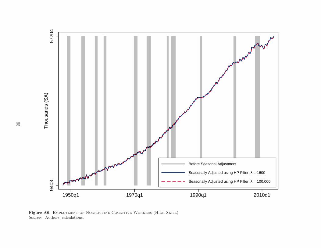
9403
5720
4T
hous
ands
(S
A)
1950q1 1970q1 1990q1 2010q1
Before Seasonal Adjustment
Seasonally Adjusted using HP Filter: λ = 1600
Seasonally Adjusted using HP Filter: λ = 100,000
Figure A6. Employment of Nonroutine Cognitive Workers (High Skill)Source: Authors’ calculations.
65

1032
634
233
Tho
usan
ds (
SA
)
1950q1 1970q1 1990q1 2010q1
Before Seasonal Adjustment
Seasonally Adjusted using HP Filter: λ = 1600
Seasonally Adjusted using HP Filter: λ = 100,000
Figure A7. Employment of Routine Cognitive Workers (Middle Skill)Source: Authors’ calculations.
66

2189
436
701
Tho
usan
ds (
SA
)
1950q1 1970q1 1990q1 2010q1
Before Seasonal Adjustment
Seasonally Adjusted using HP Filter: λ = 1600
Seasonally Adjusted using HP Filter: λ = 100,000
Figure A8. Employment of Routine Manual Workers (Middle Skill)Source: Authors’ calculations.
67

5572
2245
3T
hous
ands
(S
A)
1950q1 1970q1 1990q1 2010q1
Before Seasonal Adjustment
Seasonally Adjusted using HP Filter: λ = 1600
Seasonally Adjusted using HP Filter: λ = 100,000
Figure A9. Employment of Nonroutine Manual Workers (Low Skill)Source: Authors’ calculations.
68

9720
3174
8T
hous
ands
(S
A)
1948q1 1957q1 1966q1 1975q1 1984q1
Panel A: Nonroutine Cognitive (High Skill)
1032
627
498
Tho
usan
ds (
SA
)
1948q1 1957q1 1966q1 1975q1 1984q1
Panel B: Routine Cognitive (Middle Skill)
2189
432
783
Tho
usan
ds (
SA
)
1948q1 1957q1 1966q1 1975q1 1984q1
Panel C: Routine Manual (Middle Skill)
5651
1411
6T
hous
ands
(S
A)
1948q1 1957q1 1966q1 1975q1 1984q1
Panel D: Nonroutine Manual (Low Skill)
Historical Series with All Age, Classification−Break, and Seasonal Adjustments
Series Published in BLS Bulletin 2096 (1982)
Figure A10. Comparison of Occupational Employment Series with Published Series from BLS Bulletin 2096: 1958:Q1–1981:Q4Source: Authors’ calculations. Note: All data are seasonally adjusted. Constructed employment series were seasonally adjusted using an HP filterwith smoothing parameter λ = 100,000.
69

12
34
56
Per
cent
of L
abor
For
ce
1960q1 1970q1 1980q1 1990q1 2000q1 2010q1
Panel A: Nonroutine Cognitive (High Skill)
24
68
10P
erce
nt o
f Lab
or F
orce
1960q1 1970q1 1980q1 1990q1 2000q1 2010q1
Panel B: Routine Cognitive (Middle Skill)
510
1520
Per
cent
of L
abor
For
ce
1960q1 1970q1 1980q1 1990q1 2000q1 2010q1
Panel C: Routine Manual (Middle Skill)
46
810
12P
erce
nt o
f Lab
or F
orce
1960q1 1970q1 1980q1 1990q1 2000q1 2010q1
Panel D: Nonroutine Manual (Low Skill)
1957=1967 E&E; 1958−82=Bull 2096 (SA)
Using OCC1950 and CPS Microdata (16+, NSA)
Figure A11. Raw Data for Unemployment RatesSource: Authors’ calculations. Note: The source for the blue lines are Bulletin 2096, except for rates from 1957, which come from the March 1967Employment and Earnings. The source of the red lines are CPS microdata using the OCC1950 coding system.
70

2030
4050
60M
illions (NS
A)
2030
4050
60M
illio
ns (
NS
A)
1970q1 1980q1 1990q1 2000q1 2010q1
Panel A: Nonroutine Cognitive (High Skill)
2025
3035
40M
illions (NS
A)
2025
3035
40M
illio
ns (
NS
A)
1970q1 1980q1 1990q1 2000q1 2010q1
Panel B: Routine Cognitive (Middle Skill)
2628
3032
3436
Millions (N
SA
)
2628
3032
3436
Mill
ions
(N
SA
)
1970q1 1980q1 1990q1 2000q1 2010q1
Panel C: Routine Manual (Middle Skill)
1015
2025
30M
illions (NS
A)
1015
2025
30M
illio
ns (
NS
A)
1970q1 1980q1 1990q1 2000q1 2010q1
Panel D: Nonroutine Manual (Low Skill)
Defined as in 1947q3−2013q4 analysis using published data
Defined as in Autor (2010) & Acemoglu−Autor (2011) using CPS microdata
Figure A12. Comparison of Historical Data with CPS Microdata coded as in Autor (2010) and Acemoglu and Autor (2011)Source: Authors’ calculations. Note: On the vertical axes, “NSA” means “not seasonally adjusted.”
71


